Chemical abundances in Sgr A East: evidence for a Type Iax supernova remnant

Abstract

Recent observations have shown a remarkable diversity of observational behaviors and explosion mechanisms in thermonuclear supernovae (SNe). An emerging class of peculiar thermonuclear SNe, called Type Iax, show photometric and spectroscopic behaviors distinct from normal Type Ia. Their origin remains highly controversial, but pure turbulent deflagration of white dwarfs (WDs) has been regarded as the leading formation theory. The large population of Type Iax indicates the existence of unidentified Galactic Type Iax supernova remnants (SNRs). We report evidence that SNR Sgr A East in the Galactic center resulted from a pure turbulent deflagration of a Chandrasekhar-mass carbon–oxygen WD, an explosion mechanism used for Type Iax SNe. Our X-ray spectroscopic study of Sgr A East using 3 Ms of Chandra data shows a low ratio of intermediate-mass elements to Fe and large Mn/Fe and Ni/Fe ratios. This abundance pattern does not accord with the core-collapse or normal Type Ia models. Sgr A East is thus the first Galactic SNR for which a likely Type Iax origin has been proposed and the nearest target for studying this peculiar class. We compared Sgr A East with the Fe-rich SNRs 3C 397 and W49B, which also have high Mn and Cr abundances and were claimed to result from deflagration-to-detonation explosions of Chandrasekhar-mass WDs (although with disputes). Our study shows that they have distinct abundance patterns. The X-ray spectroscopic studies of thermonuclear SNRs provide observational evidence for the theories that there are diverse explosion channels and various metal outputs for Chandrasekhar-mass WDs.

1 Introduction

Thermonuclear supernovae (SNe) are factories of iron-group elements (IGEs, such as Fe, Ni, Mn, Cr) in our universe, but their metal yields are sensitive to the explosion mechanisms (e.g., Seitenzahl & Townsley, 2017). Recent observations have shown that the thermonuclear SN zoo includes more than Type Ia SNe (see Jha et al., 2019, for a recent review). The observed diversity provides opportunities to study different explosion mechanisms of white dwarfs (WDs).

Type Iax SNe are the largest class of peculiar thermonuclear SNe with observational behaviors similar to SN 2002cx, which was initially considered as the most peculiar Type Ia SN (Li et al., 2003). They are distinguished from normal Type Ia because they show lower luminosities and ejecta velocities and masses, implying that the Type Iax and Type Ia classes are created from different explosion mechanisms (Foley et al., 2013).

The current understanding of Type Iax SNe has only been obtained from extragalactic SNe, lacking observations of detailed chemical composition in SN ejecta. Their origin has been highly controversial (e.g., Lyman et al., 2013; McCully et al., 2014) and their later evolution has not been observed in detail. Among those controversial models for Type Iax SNe, promising are the pure deflagration models of a WD with a bound remnant (see Jha, 2017, for a review), which predict that the ejecta has large Mn, Cr, and Ni to Fe ratios, but a low ratio of intermediate-mass elements (IMEs) to Fe (Fink et al., 2014; Leung & Nomoto, 2020a).

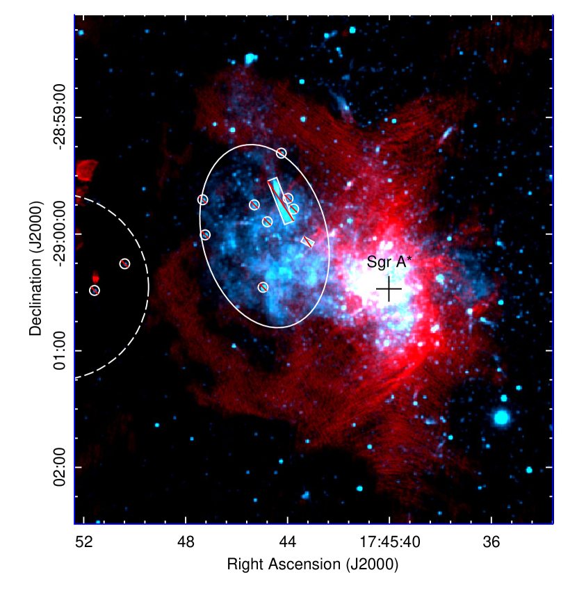
Figure 1: Composite image of Sgr A East. Red:VLA 8.3 GHz image (Zhao et al., 2009); Cyan: Chandra 2–8 keV image. The spectral extraction region (solid) and background region (dashed) are overlaid. The small circles and rectangles denote bright point sources and nonthermal filaments that are probably interlopers and thus masked from spectral extraction.

The population of Type Iax is found to be large, with 2–5 for every 10 Type Ia (Foley et al., 2013). Finding a remnant of a nearby Type Iax SN would provide essential insight into this group. However, none of 294–383 known Galactic supernova remnants (SNRs; Green, 2017; Ferrand & Safi-Harb, 2012) has been reported to have a Type Iax origin. The Type Ia SN rate of $19\pm 6\%$ (Li et al., 2011) could be translated to $\sim 40$–100 Type Ia SNRs in our Galaxy. Given the large occurrence rate of Type Iax SNe, we roughly estimate that a few to $\sim 50$ Type Iax SNRs in our Galaxy are waiting to be identified.

Sgr A East (G0.0+0.0) is the only known SNR strikingly close to the Galactic-center super-massive black hole, originally identified from radio observations (Ekers et al., 1983). A few arguments support that Sgr A East is interacting with the molecular ridge in the central parsecs and is likely overrunning the circumnuclear disk orbiting the supermassive black hole Sgr A* (see Figure 1 and Rockefeller et al., 2005). Sgr A East has been presumed to result from a core-collapse SN explosion of a $<20~{}M_{\odot}$ star (Maeda et al., 2002; Park et al., 2005), although a Type Ia origin has not been ruled out, as Fe is found to be more abundant than IMEs in the remnant (Sakano et al., 2004; Park et al., 2005). Ono et al. (2019) reported Mn and Cr lines from Sgr A East using Suzaku data. Mn and Cr are more frequently observed in thermonuclear SNRs (see Yang et al., 2013, and references therein), although they have also been found in the X-ray-luminous core-collapse SNR Cassiopeia A (e.g., Sato et al., 2020b).

SNR origin can often be probed through metal composition in the ejecta as diagnosed by X-ray spectroscopy (Vink, 2012). We utilize the 3 million second (Ms) Chandra X-ray data taken in 2012, with a total exposure more than five times that of any previous X-ray studies. The deep observations allow us to clearly detect lines such as Mn, Cr, and Fe and use the metal composition of the remnant to unveil its SN origin.

The paper is organized as follows. Section 2 describes the Chandra X-ray data used for this study. The analysis of the X-ray data is presented in Section 3. In Section 4, we compare the abundance pattern of Sgr A East with various SN nucleosynthesis models and discuss its Type Iax origin. This section also includes a discussion about Sgr A East has distinguished abundances from 3C 397 and W49B, two middle-aged SNRs that also show high abundances of Mn, Cr, and Fe and were proposed to have a thermonuclear SN origin (Yamaguchi et al., 2015; Zhou & Vink, 2018).

2 Chandra X-ray Data

The inner parsecs of the Galactic center, where Sgr A East is located, have been frequently observed by the Chandra X-ray observatory, primarily with its Advanced CCD Imaging Spectrometer (ACIS). In this work, we utilized a total of 38 observations taken in 2012 for spectroscopic analysis. These observations were taken with the combined operation of ACIS-S and the High Energy Transmission Grating (HETG), in a total exposure of 2.94 Ms. With the HETG inserted, about one half of the incident X-rays are dispersed, while the remaining X-rays continue to the detector directly and form the “zeroth-order” image. We used only data from the “zeroth-order” image (here referred to as the ACIS-S image for simplicity). While there also exist a large number of ACIS-I observations toward the Galactic center, we do not include these data for two reasons: (1) in most cases, Sgr A East falls on the CCD gaps of the ACIS-I array, potentially introducing systematic uncertainty in the instrumental response; (2) it is known that charge-transfer inefficiency degrades the spectral resolution of ACIS, in the sense that signals recorded in larger detector rows have a poorer resolution. Therefore, at the position of Sgr A East, the ACIS-S observations have a better spectral resolution than that of the ACIS-I, which is desirable for accurate measurement of emission lines expected from the hot plasma. To maximize the X-ray photons shown in Figure 1, we combined the ACIS-S image taken in 2012 and the ACIS-I image taken during 1999 and 2013. The detailed observation information is listed in Table 1 in Zhu et al. (2018).

We uniformly reprocessed the archival data with CIAO v4.10 and calibration files CALDB v4.7.8, following the procedures detailed in Zhu et al. (2019). We have examined the light curve of each ObsID and, when necessary, removed time intervals contaminated by particle flares. We use XSPEC (Arnaud, 1996, vers 12.10.1f) with ATOMDB 3.0.9 for spectral analysis.

3 Spectral analysis

We extracted the global spectrum from the X-ray-bright region in the SNR interior (the solid ellipse with a short half-axis of $32^{\prime\prime}$ and a long half-axis of $48^{\prime\prime}$, in Figure 1) and subtracted the background from a source-free region outside the SNR boundary (the dashed circle). We removed several bright point-like sources with an observed 2-8 keV photon flux greater than $8\times 10^{-7}{\rm~{}photons~{}cm^{-2}~{}s^{-1}}$ and two nonthermal filaments. We coadded the 38 individual spectra to produce a combined spectrum of high signal-to-noise ratio, weighting the corresponding ancillary response files (ARFs) and redistribution matrix files (RMFs) by the effective exposure.

Figure 2 shows the ACIS S3-chip spectrum of Sgr A East extracted from the X-ray-bright interior (see Figure 1). The combined spectrum of Sgr A East in 2–8 keV shows emission lines of S, Ar, Ca, Fe, and Ni. We confirm that Cr and Mn He$\alpha$ lines are detected at 5.63 keV and 6.13 keV, respectively (Ono et al., 2019). The Fe He$\alpha$ and Ly$\alpha$ lines are also separated using the ACIS-S chips, while the ACIS-I cannot resolve them (see ACIS-I spectra in Park et al., 2005).

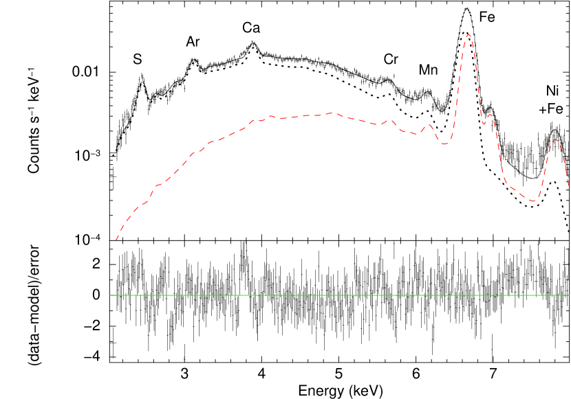
Figure 2: Chandra ACIS-S spectrum in 2–8 keV fitted with an absorbed two-temperature model $tbabs*(vvapec+vvapec)$. The dotted line and the red dashed line denote the cool and hot components, respectively. Spectral fit results are shown in Table 1.

We first summarize the best-fit results of our spectral analysis, followed by a detailed description of the spectral fit in Sections 3.1 and 3.2. We found that a two-temperature plasma model can well describe the X-ray spectrum, providing a reduced $\chi^{2}$ of $\chi_{\nu}^{2}=1.45$ with a degree of freedom (dof) of 381 (see Figure 2), while none of the single thermal models can fit the spectrum well ($\chi_{\nu}^{2}\gtrsim 2$, see Table 1). The X-ray emission is characterized by a cool component with a temperature $kT_{\rm c}=1.19\pm 0.03$ keV and a hot component with a temperature $kT_{\rm h}=4.3\pm 0.2$ keV, with a foreground absorption of $N_{\rm H}=2.14\pm 0.04\times 10^{23}~{}\,{\rm cm}^{-2}$. Both components are in (near-)collisional ionization equilibrium (CIE). The two temperatures are consistent with those suggested in previous X-ray studies of Sgr A East (Sakano et al., 2004; Park et al., 2005). Moreover, we found very high abundances of IGEs Cr ($5.6\pm 1.0$), Mn ($17\pm 3$), Fe ($6.5\pm 0.4$), and Ni ($17\pm 4$) compared with solar abundances. Quoted errors here are at a 90% confidence level. The uncertainty of the Ni abundance could be larger than the fitted value as residuals ($\lesssim 2\sigma$) are shown in 7–8 keV. In contrast, the IMEs S, Ar, and Ca have ordinary abundances ($1.4\pm 0.2$, $1.5\pm 0.2$ and $1.7\pm 0.1$, respectively), which are similar to the mean interstellar medium values of $\sim 2$ in the Galactic center (Mezger et al., 1996), and consistent with the S and Ca abundances obtained from the observations of HII regions ($Z_{\rm S}/Z_{\rm S}^{\odot}\sim 1.5$, Rudolph et al., 2006) and red supergiants ($Z_{\rm Ca}/Z_{\rm Ca}^{\odot}\sim 1.7$, Davies et al., 2009).

Table 1: Best-fit results of the global spectrum with 90% uncertainties

Energy Range	2–8 keV			5–8 keV
Model	$vvnei+vvapec$	$vvapec+vvapec$		$vvapec$	$vvrnei$	$bvvrnei^{a}$
$\chi_{\nu}^{2}$/dof	1.43/380	1.45/381		3.94/188	3.00/186	1.95/185
$N_{\rm H}(10^{23}$ cm${}^{-2})$	$2.07\pm 0.05$	$2.14\pm 0.04$		2.14 (fixed)	2.14 (fixed)	2.14 (fixed)
$kT_{\rm c}$ (keV)	$1.22\pm 0.04$	$1.19\pm 0.03$		$\sim 1.62$	$\sim 1.52$	$1.52\pm 0.03$
$kT_{\rm c}^{\rm init}$ (keV)	…	…		…	$\sim 11.7$	$>7.7$
$\tau_{\rm c}~{}(10^{11}$ cm-3 s)b	$>7.2$	…		…	$\sim 8.8$	$8.5^{+1.8}_{-1.4}$
$kT_{\rm h}$ (keV)	$4.0\pm 0.2$	$4.3\pm 0.2$		…	…	…
$norm_{\rm c}(\times 10^{-2})$	$4.4\pm 0.4$	$4.8\pm 0.3$		$\sim 3.4$	$\sim 3.8$	$3.9\pm 0.2$
$norm_{\rm h}(\times 10^{-3})$	$2.6\pm 0.3$	$2.0\pm 0.3$		…	…	…
S c	$1.4\pm 0.2$	$1.4\pm 0.2$		…	…	…
Ar	$1.5\pm 0.2$	$1.5\pm 0.2$		…	…	…
Ca	$1.7\pm 0.1$	$1.7\pm 0.1$		…	…	…
Cr	$4.7\pm 1.0$	$5.6\pm 1.0$		$\sim 2.7$	$\sim 3.6$	$3.0\pm 0.6$
Mn	$14.5\pm 2.5$	$16.9\pm 2.6$		$\sim 8.7$	$\sim 10.7$	$9.0\pm 1.2$
Fe	$6.2\pm 0.3$	$6.5\pm 0.4$		$\sim 4.3$	$\sim 4.0$	$3.5\pm 0.2$
Ni	$14.6\pm 3.1$	$17.0\pm 3.5$		$\sim 20$	$\sim 17$	$12.4\pm 2.3$

• ^a In the $bvvrnei$ model, the best-fit Gaussian sigma for the velocity broadening is $1.44\pm 0.09\times 10^{3}\,{\rm km}\,{\rm s}^{-1}$.

• ^b The ionization timescale $\tau_{c}=\int n_{e}dt\sim n_{e}t$ for the underionized plasma model $vvnei$ model or recombining timescale for the recombining plasma $bvvrnei$ model. It describes an electron density $n_{e}$-weighted timescale, starting from an instantaneous heating ($vvnei$) or cooling ($vvrnei$).

• ^c The abundance ratio of the element relative to its solar value (e.g, for S, the value means $Z_{\rm S}/Z_{\rm S}^{\odot}$).

3.1 Single-component model

We first investigated the hard X-ray emission in 5–8 keV, where IGE (Cr, Mn, Fe, and Ni) lines are shown. As the hard X-ray spectrum cannot well constrain $N_{\rm H}$, we fixed $N_{\rm H}$ value to $2.14\times 10^{23}~{}\,{\rm cm}^{-2}$, the best-fit result from fitting the 2–8 keV spectrum with a two-temperature model. Table 2 shows the line properties of Cr, Mn, and Fe, which are obtained by simply fitting the 5–8 keV spectrum with an absorbed bremsstrahlung component plus Gaussian lines (see Figure 3). The photon fluxes for the Cr and Mn lines are around $3\times 10^{-6}$ photon s^-1 cm^-2. The Fe Ly$\alpha$ to He$\alpha$ intensity ratio of 3% implies an ionization temperature of $\sim 3.0$ keV (ATOMDB 3.0.9), which is higher than the electron temperature of $2.0\pm 0.1$ keV obtained from the bremsstrahlung continuum. This implies that either the gas is overionized or the X-ray plasmas have multitemperature components.

Table 2: Line properties for the Fe-group elements and the 90% uncertainties

Line	Central Energy	Widtha	Photon Flux
	(keV)	(eV)	(photons s-1 cm-2)
Cr He$\alpha$	$5.63\pm 0.02$	…	$3.2\pm 0.8\times 10^{-6}$
Mn He$\alpha$	$6.13\pm 0.02$	…	$2.8\pm 0.7\times 10^{-6}$
Fe He$\alpha$	$6.654\pm 0.001$	$45\pm 1$	$2.03\pm 0.02\times 10^{-4}$
Fe Ly$\alpha$	$6.978\pm 0.003$	…	$6.6\pm 0.9\times 10^{-6}$
Ni He$\alpha$+Fe lines	$7.82\pm 0.02$	$138^{+41}_{-26}$	$3.0^{+0.5}_{-0.3}\times 10^{-5}$

Note. — ^a The Cr He$\alpha$, Mn He$\alpha$ and Fe Ly$\alpha$ lines are narrow, and their widths cannot be constrained.

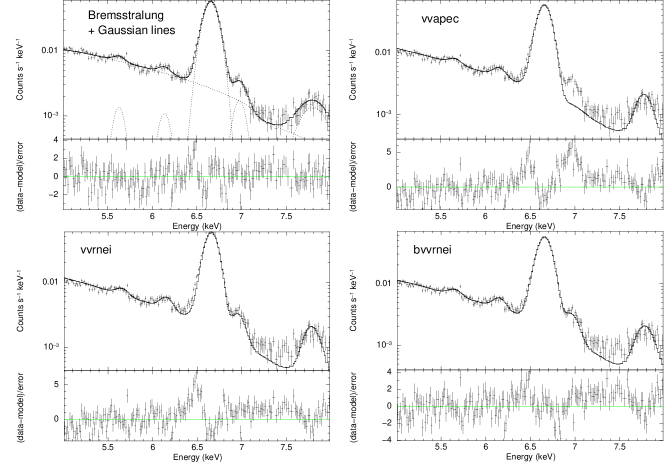
Figure 3: Chandra ACIS-S spectrum in 5–8 keV fitted with single thermal component models. Top left: the spectrum in 5–8 keV fitted using absorbed bremsstrahlung$+$Gaussian lines (see Table 2 for the fitting results); top right: $vvapec$; bottom left: recombining plasma model $vvrnei$; and bottom right: recombining plasma model $bvvrnei$ with a velocity broadening.

We subsequently tried to fit the spectrum with single thermal plasma models, including an absorbed CIE model ($vvapec$) and an absorbed recombining plasma model ($vvrnei$). The Tuebingen–Boulder interstellar medium (ISM) absorption model $tbabs$ is adopted to account for foreground absorption. The latest measurements of solar abundances ($aspl$ in XSPEC) are used (Asplund et al., 2009). Neither of the single-temperature models provides an acceptable fit to the Fe emission, despite the fact that the $vvrnei$ model better describes the Fe Ly$\alpha$ emission (see the best-fit results in Table 1). As shown in Figure 3, the Fe He$\alpha$ line (with a width of $45\pm 1$ eV) is too wide to be explained with the two single-temperature models. Using a velocity-broadened recombining model $bvvrnei$ improves the fit, but strong residuals are still shown, giving a large $\chi_{\nu}^{2}=1.95$. This prompted us to use a two-temperature model, which is often suited for SNRs.

3.2 Two-temperature model

A two-temperature component is needed to fit the spectrum in the 2–8 keV band, as pointed out in previous studies (Sakano et al., 2004; Park et al., 2005; Koyama et al., 2007; Ono et al., 2019). We found that an absorbed two-temperature plasma model $vvapec+vvapec$ with abundances tied together well describes the spectrum in the 2–8 keV band and provides a reduced $\chi^{2}$ ($\chi^{2}_{\nu}$) of 1.45 (dof=381). This model suggests that the elements between the cool and hot components are well mixed. The best-fit results for the $vvapec+vvapec$ model with 90% uncertainties are shown in Table 1.

Here we explain why the abundances of the two components are tied. First, we tested the unmixed case by freeing the abundances of IGEs in the hot component and fixing the abundances of IGEs in the cool component to the ambient value (1 or 2). This model results in a bad fit ($\chi^{2}_{\nu}\sim 2.8$), because the spectral fit is sensitive to the Fe abundance in both components. A low Fe abundance in the cool component causes large residuals in the Fe He$\alpha$ and Ly$\alpha$ lines. Hence, both the cold and hot components contain SN ejecta. Second, the element abundances in the hot component cannot be independently constrained because of a strong degeneracy with the cold component. The best-fit abundances are mainly determined by the cold component, which dominates the photons below 6.7 keV (see Figure 2). Separating the abundances of the two components will invoke manual tuning of the hot component’s abundances. This requires knowledge of how unmixed the ejecta is, which we do not know. Finally, coupling the abundances of two ejecta components is based on the simplest and natural consideration: the ejecta is well mixed. In this case, the cool component corresponds to the denser clumps, while the hot component is from the intercloud gas (see further discussion about the plasma in Appendix B). Therefore, we tied the abundances between the cool and hot components and allow the abundances of S, Ar, Ca, Cr, Mn, Fe, and Ni to vary. This further supports the previous XMM-Newton and Chandra studies, which used the same abundances in two-temperature components (Sakano et al., 2004; Park et al., 2005).

We also tested the underionized ($vvnei$) and recombining plasma models ($vvrnei$) for the cool and hot components. We found that the hot component is in CIE, given the large ionization or recombining timescale ($>10^{13}~{}\,{\rm cm}^{-3}\,{\rm s}$) in the $vvnei$ and $vvrnei$ models. The cold component could also be fitted using an underionized model $vvnei$ with a large ionization timescale of $\tau_{c}>0.7\times 10^{12}\,{\rm cm}^{-3}\,{\rm s}$, implying a CIE condition (Smith & Hughes, 2010). The $vvnei+vvapec$ two-temperature model gives best-fit parameters and $\chi_{\nu}^{2}(=1.43$) similar to the $vvapec+vvapec$ model. Therefore, it is equivalent to use the $vvapec+vvapec$ model as the best model.

Finally, we compared our results with earlier X-ray studies of Sgr A East. Our best-fit model, plasma temperature, and metal abundances of IME and Fe are consistent with the previous Chandra study by Park et al. (2005), but we added the Cr, Mn, and Ni abundances and provided better constraints for all parameters with deep Chandra observations. Our best-fit temperatures are similar to that from the XMM-Newton study by Sakano et al. (2004), which also suggests low abundances of S, Ar, and Ca ($Z/Z^{\odot}=1$–3). We found larger differences between our Chandra results and the Suzaku results by Ono et al. (2019), which requires two recombining plasma models with different IGE abundances. This large discrepancy is likely caused by the different spectral extraction regions. The elliptical region shown in Figure 1 has a size of $1^{\prime}\times 1\farcm{5}$, while the Suzaku spectrum in Ono et al. (2019) was selected in a $3\farcm{2}$-diamter region. Due to the larger point spread function of Suzaku ($\sim 1^{\prime}$ or worse, Ono et al., 2019), the Suzaku spectrum of Sgr A East suffers more contamination from background structures such as nonthermal filaments, bright point-like sources, and other irrelevant emission near Sgr A*.

The previous Chandra and XMM-Newton studies have a revealed a spatial variation of physical parameters across Sgr A East. This paper focuses on the global properties of Sgr A East, especially for the abundance ratios. In the appendix, we have extracted spectra from three regions across Sgr A East. Despite a variation of gas temperature, the abundance ratios of the IGEs are still consistent with the global spectrum.

4 Discussion

4.1 Comparison with SN nucleosynthesis models

The abundance pattern of Sgr A East suggests that its progenitor SN produced mainly IGEs but little IMEs of S, Ar, and Ca. This pattern is surprising and is remarkably distinct from other known SNRs. The two main categories of SNRs are Type Ia SNRs from C+O WDs and core-collapse SNRs from massive stars. Both SN categories produce a moderate amount of IMEs relative to IGEs, and especially core-collapse SNe produce much more IMEs.

In order to probe the explosion mechanism of Sgr A East, we compare the logarithmic abundance ratios in Sgr A East with those predicted in several nucleosynthesis models of SNe (see Figures 4 and 5). The logarithmic abundance ratio of element Z to Fe is defined as [Z/Fe]= $\log_{10}(Z_{\rm Z}/Z_{\rm Fe})-\log_{10}(Z_{\rm Z}/Z_{\rm Fe})^{\odot}$. Sgr A East has logarithmic abundance ratios [Cr/Fe] $=-0.065^{+0.075}_{-0.091}$, [Mn/Fe] $=0.41^{+0.07}_{-0.08}$, [Ni/Fe] $=0.42^{+0.08}_{-0.11}$, [S/Fe] $<-0.60$, [Ar/Fe] $<-0.58$, and [Ca/Fe] $<-0.55$. In this paper, we also use abundance ratios defined as Z/Fe = $(Z_{\rm Z}/Z_{\rm Fe})/(Z_{\rm Z}/Z_{\rm Fe})^{\odot}$.

The contamination of the ambient gas to the SN ejecta is considered in the comparison. The clearly enhanced abundances of IGEs support that the IGEs are dominated by the ejecta component. Contrarily, the S, Ar, and Ca abundances are close to the average values in the Galactic center (Mezger et al., 1996; Rudolph et al., 2006; Davies et al., 2009), indicating small S/Ar/Ca yields from the SN and a strong dilution with the ISM. Therefore, the [(Cr, Mn, Ni)/Fe] ratios represent the ejecta values and can be directly compared with the models. Since the S, Ar, and Ca abundances are close to the ambient value, the abundance ratios of IMEs to Fe in Figures 4 and 5 are given as the upper limits.

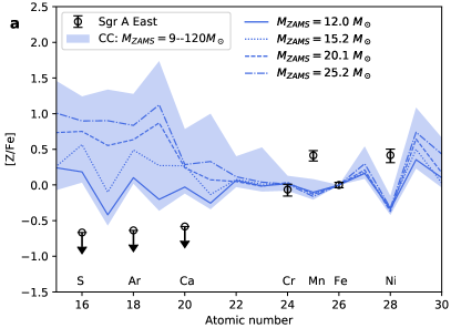
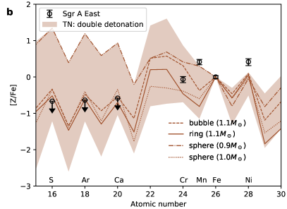
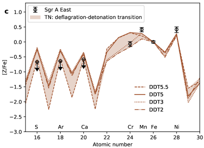
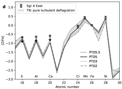
Figure 4: A comparison between the observed logarithmic abundance ratios (relative to Fe) and core-collapse (CC) and thermonuclear (TN) nucleosynthesis models. The error bars give 90% uncertainties. (a) core-collapse SN models for stars with zero-age-main-sequence masses from 9 to 120 $M_{\odot}$ (Sukhbold et al., 2016). (b) double detonation Type Ia models for sub-Chandrasekhar-mass WDs (0.9–1.2 $M_{\odot}$) with three initial He detonation configurations (Leung & Nomoto, 2020b). Three benchmark models and a low-mass WD model ($0.9~{}M_{\odot}$ WD) are labeled with lines. (c) deflagration-detonation transition (DDT) Type Ia SN models for C+O WDs with central densities of $2\times 10^{9}$ (DDT2), $3\times 10^{9}$ (DDT3), $5\times 10^{9}$ g cm^-3 (DDT5), and $5.5\times 10^{9}$ g cm^-3 (DDT5.5), respectively (Leung & Nomoto, 2018). (d) pure turbulent deflagration (PTD) Type Iax SN models (Leung & Nomoto, 2020a) for WDs with central densities in the range of 2.0–$5.5\times 10^{9}$ g cm^-3 (PTD2–5.5). The thick solid line shows the best-fit Type Iax model with a central density of $5\times 10^{9}$ g cm^-3.

4.1.1 Core-collapse models

In Figure 4a, we compared the observation with core-collapse SN models by Sukhbold et al. (2016) (see also Nomoto et al., 2013, for independent and consistent yields). It shows that the core-collapse SN origin of Sgr A East can be ruled out as it would overproduce IMEs relative to Fe and result in a too-small [Mn/Fe] ($-0.22$ to $0.11$) compared to the observed value of $0.41^{+0.06}_{-0.07}$.

4.1.2 Type Ia models

The observed high ratio of Mn/Fe is an important indicator for the progenitor of a thermonuclear SN, which provides conditions for the neutronization by electron capture. Such ahigh Mn/Fe eliminates a sub-Chandrasekhar-mass WD progenitor because the low-density matter cannot produce both a high Mn/Fe ratio and sufficient ⁵⁶Ni for normal Type Ia SNe (Seitenzahl et al., 2013b; Shen et al., 2018; Leung & Nomoto, 2020b). In contrast, near-Chandrasekhar-mass C+O WDs have high-enough central densities for the formation of a larger amount of Mn.

Figure 4b shows a comparison between Sgr A East and the sub-Chandrasekhar-mass WD models with WD masses of 0.9–$1.2~{}M_{\odot}$ and a solar metallicity (Leung & Nomoto, 2020b). In these double detonation (DD) models, a C detonation is triggered by an initial He detonation with three different configurations. The benchmark Type Ia models are labeled with solid, dashed, and dotted lines. They represent typical sub-Chandrasekhar-mass models, reproducing $\sim 0.6~{}M_{\odot}$ ⁵⁶Ni masses and Type Ia SN explosion energies. None of them explains the observed high [Mn/Fe] and [Ni/Fe] ratios.

Among the 19 DD models, two low-mass (0.9 $M_{\odot}$ WD) models result in oversolar [Mn/Fe] and [IMEs/Fe] ratios. They are not favorable models for normal Type Ia SNe as they produce too-small ⁵⁶Ni mass ($\leq 0.14~{}M_{\odot}$). Moreover, they fail to explain the low IME abundances observed in Sgr A East.

We remind readers that Leung & Nomoto (2020b) has done a detailed survey for the parameter dependence of SNe Ia using sub-Chandrasekhar-mass WDs. The WD mass and metallicity (0–5$Z_{\odot}$) are the primary parameters that affect the global abundance pattern. To achieve the supersolar [Mn/Fe] ratio, for sub-Chandrasekhar-mass WD, a low-mass or high-metallicity model is necessary. However, such a model cannot explain the subsolar IMEs/Fe ratios observed in Sgr A East, where the model shows at least 1 – 2 dex above solar values.

We thus compared Sgr A East with the near-Chandrasekhar-mass models for Type Ia and Type Iax SNe. In these models, the turbulent deflagration wave propagates initially at a slow subsonic speed from the WD center (Nomoto et al., 1976, 1984). In the deflagration-detonation transition (DDT) models by Leung & Nomoto (2018) adopted here (see Röpke et al., 2007, for a review), the transition from the deflagration to the supersonic detonation is assumed to occur at a density as low as $\sim 10^{7}$ g cm^-3. In the pure turbulent deflagration (PTD) models, it is assumed that the transition from the deflagration to detonation does not occur.

For comparison with Sgr A East, we applied the theoretical yields of the two-dimensional DDT models (Leung & Nomoto, 2018) and newly calculated two-dimensional PTD models (Leung & Nomoto, 2020a). These yields are given in Tables 5–6 in the appendix. Our discussion focuses on these two recent models with centered flame structures, followed by a brief comparison with earlier models with other flame structures by Seitenzahl et al. (2013a) and Fink et al. (2014), which assumed that the WDs are ignited with multiple flaming bubbles.

Figure 4c shows the DDT models with central densities of $2$–$5.5\times 10^{9}$ g cm^-3 (models DDT2–5.5, Leung & Nomoto, 2018). Here we added DDT2 and DDT5.5, which were not included in Leung & Nomoto (2018). We noted the following from Figure 4c: (1) DDT2, DDT3, DDT5, and DDT5.5 produce [Mn/Fe] and [Ni/Fe] values that are a little smaller than the observation; (2) DDT5 and DDT5.5 produce too-large [Cr/Fe] to be compatible with the observation; (3) DDT2 and DDT3 reproduce the observed [Cr/Fe] but overproduce IMEs relative to Fe. Thus, no model can explain the observed abundance pattern.

We noted that the development and assumptions in SN nucleosynthesis models could affect the interpretation of the SNR origin. To investigate the dependence on hydrodynamics and nucleosynthesis models, we also compared with the three-dimensional DDT models from Seitenzahl et al. (2013a), which assumed that the Chandrasekhar-mass WDs are ignited by multiple off-center flaming bubbles (up to 1600). None of the models could explain both the low abundances of the IMEs and the large Mn/Fe ratio in Sgr A East(see Figure 5a). The N1600 model for strong deflagration with 1600 ignition bubbles is the only one reproducing the IGE/Fe ratios, but it largely overproduces IME/Fe ratios.

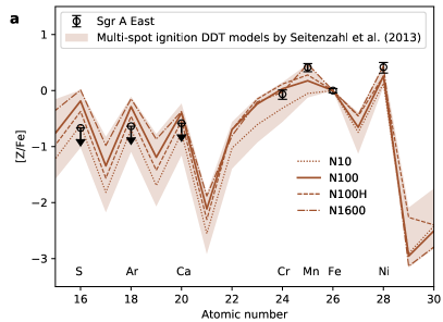
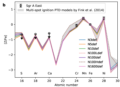
Figure 5: Comparison between the observed logarithmic abundance ratios (relative to Fe) and offcentered mutispot ignition DDT (a) and PTD models (b). All available models have been considered in the shaded region, but a few exemplified models are shown with lines. N10(def) and N100(def) mean 10 and 100 ignition bubbles, respectively. In panel (b), the initial central density of the WD is $2.9\times 10^{9}~{}\,{\rm g}\,{\rm cm}^{-3}$ for the N3–1600def models, $10^{9}~{}\,{\rm g}\,{\rm cm}^{-3}$ for the N100Ldef model and $5.5\times 10^{9}~{}\,{\rm g}\,{\rm cm}^{-3}$ for the N100Hdef model.

4.1.3 Pure turbulent deflagration Type Iax models

Lastly, in Figure 4d, we examined the PTD models, which have been suggested to be the most likely mechanism to explain the properties and large observational diversities in Type Iax SNe (e.g., Branch et al., 2004; Fink et al., 2014; Leung & Nomoto, 2018). Here we studied the dependence on the central density of the WD by adopting the two-dimensional hydrodynamical models PTD2, PTD3, PTD5, and PTD5.5 for the central densities of 2, 3, 5, and 5.5 $\times 10^{9}$ g cm^-3, respectively (Table 6 and Leung & Nomoto, 2020a). According to these PTD models, the subsonic slow propagation of the turbulent deflagration wave cannot sustain its burning and quenches, because the density at the burning front decreases with the expansion of the WD. Then the WD cannot be completely disrupted, and a low-mass WD remnant is left behind the SN explosion. The absence of supersonic detonation suppresses the formation of IMEs at such low densities as $\sim 10^{7}$ g cm^-3. Because of turbulent mixing associated with the deflagration, the ejecta of PTD models contain IGEs that are synthesized in the high-density central region of the WD. Compared with DDT models, the ejecta of PTD models show much smaller IME/Fe ratios, which are consistent with the observed upper limits to these ratios.

From Figure 4d, we found that the ratios of [(Cr, Mn, Ni)/Fe] observed in Sgr A East are well explained by the PTD5 and PTD5.5 models, that is, the explosions of WDs with central densities of 5 and 5.5 $\times 10^{9}$ g cm^-3, respectively. The best-fit model PTD5 (see Figure 4d) predicts that the explosion energy is $5.1\times 10^{50}$ erg and the ⁵⁶Ni mass is $0.32M_{\odot}$ (Leung & Nomoto, 2020a). These predictions could explain a relatively bright Type Iax SN (Foley et al., 2013; Stritzinger et al., 2015).

The central densities at the deflagration of the accreting WDs basically depend on the accretion rate (Nomoto & Leung, 2018). The densities of the PTD5 and PTD5.5 models ($5$ – $5.5\times 10^{9}$ g cm^-3) are somewhat higher than the typical central densities ($2-3\times 10^{9}$ g cm^-3) of normal Type Ia SN models. Such high densities at the deflagration could be obtained by the thermonuclear runaway of a uniformly rotating WD ($5-6\times 10^{9}$ g cm^-3) whose mass reaches $\sim 1.43~{}M_{\odot}$ in the (so-called) spin up – spin down scenario (Benvenuto et al., 2015).

The PTD5 model can bring an ejecta mass of $\sim 1.3~{}M_{\odot}$. This includes a significant amount of cold fuel made of ¹²C and ¹⁶O. In fact, the ejecta mass is sensitive to how the initial flame is arranged. The PTD2–5.5 models assumed the flame starts at the center with angular perturbation. This flame structure refers to that presented in Reinecke et al. (1999, 2002) for a robust mass ejection without invoking the detonation transition. The centered flame allows the flame to steadily burn the core for the steady expansion before the flame is quenched. The initial burning of the core provides the necessary thermodynamical conditions for electron capture and synthesis of neutron-rich isotopes, including ⁵⁵Mn.

Other flame structures, such as off-center flame bubbles, are presented in Fink et al. (2014). The off-center flame encountered strong a buoyancy force, which drags the flame away from the center before it can sweep through the matter around the core. A drastically lower ejecta mass can result.

In Figure 5b, the abundance ratios of PTD models by Fink et al. (2014) are compared with Sgr A East. These models assumed that the WDs are ignited by many bubbles with number $N_{k}=1$ – 1600. In the models N3def–N1600def (solid lines) with a WD central density of $2.9\times 10^{9}$ g cm^-3, the predicted abundance patterns are marginally consistent with that in Sgr A East.

We then compare with N100Hdef, which has a central density of $5.5\times 10^{9}$ g cm^-3 at the ignition. It predicts a higher [Cr/Fe], with the Cr and Fe yields similar to the PTD5.5 model by Leung & Nomoto (2020a). The comparison in Figure 5b implies a central density of 3–$5\times 10^{9}~{}\,{\rm g}~{}\,{\rm cm}^{-3}$ for the WD progenitor of Sgr A East, marginally consistent with the central density suggested by the PTD5–5.5 models (see Figure 4d). This agreement reinforces that Sgr A East has an abundance pattern typical for PTD of WDs, no matter how the initial flame structures appear.

Fink et al. (2014) made comparisons of models with the observed light curves and spectra of SNe Iax and found that the weaker and fainter explosion models with $N_{k}=5$ and 10 are better than larger $N_{k}$ models for explaining SN 2002cx-like Type Iax SNe. Long et al. (2014) also performed a three-dimensional simulation for multispot PTD WDs, but they suggested a different trend: few-$N_{k}$ models producing stronger and brighter explosions (see Fink et al., 2014, for an interpretation of the difference).

Figure 5b implies that the abundance pattern, especially for [Cr/Fe], is not sensitive to the propagation velocity of the deflagration wave (related to $N_{k}$) but is sensitive to the central density. It should be useful to construct high-central-density models, like PTD5 and PTD5.5, but with a slower deflagration (small $N_{k}$) that leads to a wide range of ejected mass (e.g., ⁵⁶Ni) and explosion kinetic energy. Since Type Iax SNe show a large variation of light curves and spectra, it would be interesting to find a range of models that can explain the wide range of observed properties of Type Iax SNe and also the chemical abundance pattern like in Sgr A East. The largest differences among the models are the metal yields, but our X-ray study cannot constrain the metal masses (a lower limit for Fe mass is $M_{\rm Fe}\sim 3\times 10^{-2}~{}M_{\odot}$; see Appendix B).

4.1.4 Other remarks on the models and abundance ratios

This paper mainly compares solar-metallicity nucleosynthesis models for consistency. The full DD and DDT models in Leung & Nomoto (2020b, 2018) have covered a wide range of progenitor metallicity ($Z=0$–5$Z_{\odot}$). These non-solar-metallicity models with WD central densities of 1–$5\times 10^{9}~{}\,{\rm g}\,{\rm cm}^{-3}$ still fail to explain the abundance pattern in Sgr A East. Moreover, the observed low IME abundances ($Z_{\rm S}/Z_{\rm S}^{\odot}=1.4\pm 0.2$) imply that high-metallicity models are not necessary for Sgr A East. For the Type Ia and Iax models, the dependence on parameters, such as the central density, metallicity, and input physics, has been extensively studied (see Leung & Nomoto, 2020b, 2018, a, with a discussion about a few other groups’ work). Appendix C provides further details about the numerical simulations of these models. Our paper has compared four explosion mechanisms, but the future development of SN models may bring a wider view.

The four explosion mechanisms used in our study can be distinguished in the [Ar/Fe]–[Mn/Fe] diagram (Figure 6). CC SNRs are mainly distributed in the second quadrant, but some may appear in the first quadrant. The DD models for sub-Chandrasekhar-mass WDs do not appear in the fourth quadrant. The PTD points are concentrated at the lower right region in the fourth quadrant, well separated from the DDT points. Sgr A East’s position in the [Ar/Fe]–[Mn/Fe] diagram favors a PTD explosion mechanism. While the diagram gives useful clues, we still suggest using a large group of elements to distinguish explosion mechanisms.

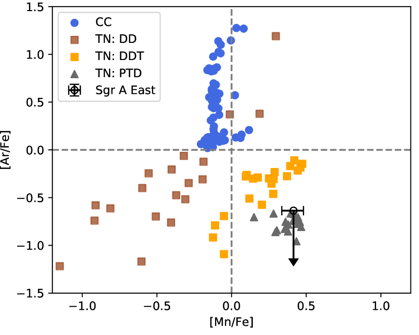
Figure 6: [Ar/Fe]–[Mn/Fe] diagram for four groups of explosion mechanisms plotted in Figures 4 and 5. The observed ratios in Sgr A East are overplotted for comparison. The dashed lines denote the solar values for [Mn/Fe] and [Ar/Fe].

4.2 Type Iax origin

Our study suggests that Sgr A East’s abundance pattern is consistent with a PTD explosion of a near-Chandrasekhar-mass WD, a leading mechanism of producing Type Iax SNe. This suggests Sgr A East could be the first identified Type Iax SNR. Type Iax SNe occur at a rate of $31^{+17}_{-13}$ for every 100 Type Ia SNe in a given volume (Foley et al., 2013). Given the large occurrence rate, we should expect to find a few or more Galactic SNRs with Type Iax origin. However, only Sgr A East has been identified so far, likely due to the difficulty of IGE measurements in old SNRs, especially for the faint lines of Mn and Cr. In our Galaxy, we have known of three confirmed Type Ia SNRs (Tycho, Kepler, and SN 1006) and two candidates (RCW 86 and G1.9+0.3) younger than 2 kyr. If Sgr A East is younger than 2 kyr (Rockefeller et al., 2005; Fryer et al., 2006), the Type Iax SNRs are found at a rate of 1 for 3–5 Type Ia SNRs in the past 2 kyr, which is consistent with the measured Type Iax SN ratio (see a detailed discussion about the dispute of the SNR age in Appendix B).

Despite the small statistics, one may wonder why the first Type Iax SNR is found near the Galactic center rather than other places in our Galaxy. The identification has been made possible by the deep Chandra observations toward the Galactic center. Type Iax SNe are preferentially found in a young environment and arise from more massive WDs with short evolution time (Lyman et al., 2013). It is suggested that the population of WDs in cataclysmic variables in the Galactic center have a mean mass of 1.2 $M_{\odot}$ (assuming non-magnetic WDs), significantly heavier than the WDs in local and Galactic-bulge cataclysmic variables ($\sim 0.8~{}M_{\odot}$, Xu et al., 2019). Although many Type Iax SNe were found in the “outskirts” of late-type galaxies (Jha et al., 2019), our study suggests that this peculiar class can also occur in the center of galaxies.

According to the PTD models, a bound remnant should be left in the explosion. It is of interest to search for the WD survivor near Sgr A East, but the high absorption toward the Galactic center brings difficulties. Recently, a few WDs with peculiar kinematics and spectroscopic properties have been identified in our Galaxy (Vennes et al., 2017; Raddi et al., 2019): they are less massive than typical WDs (only 0.14–$0.28~{}M_{\odot}$), are inflated (with radii of 0.08–$0.16R_{\odot}$), and show chemical similarities with the predicted survivors of Type Iax or thermonuclear electron-capture SNe. The studies on these inflated WDs provide another important angle for investigating peculiar thermonuclear SN explosions.

A few observations were used to indirectly argue the core-collapse origin of Sgr A East. Sgr A East was considered to be associated with the “cannonball” neutron star outside the SNR boundary (Park et al., 2005), with a transverse velocity of 500 km s^-1 (Nynka et al., 2013). This requires that the Sgr A East be an old SNR with age $\sim 10^{4}$ yr, which is inconsistent with the hydrodynamic simulations of the SNR evolution ($\lesssim 2$ kyr, Rockefeller et al., 2005; Fryer et al., 2006). Our X-ray analysis does not give any evidence for a large age of the SNR. The large ionization timescale of Sgr A East’s plasma does not necessarily support a large SNR age (see Appendix B, and see Ono et al., 2019, for a few possible explanations of the high ionization state of the plasma). Yalinewich et al. (2017) found that Sgr A East in the Galactic center evolves faster than other Galactic SNRs, and it cannot be an old SNR associated with the “cannonball” neutron star. Furthermore, the abundance pattern of Sgr A East suggests a WD survivor but excludes a neutron star survivor. Therefore, the association of the “cannonball” has not been established to imply a core-collapse origin for Sgr A East.

Several earlier X-ray studies considered a core-collapse origin for Sgr A East (Maeda et al., 2002; Park et al., 2005), but these studies did not present a comparison between all of the constrained metal abundances and different SN nucleosynthesis models. As shown in Figure 4, the core-collapse models have severe problems in Sgr A East, as they produce too much IMEs and too little Mn and Ni to Fe. Sakano et al. (2004) pointed out that Type Ia may explain why Fe is more abundant than IMEs, although they did not exclude a Type II. Park et al. (2005) constrained the maximum Fe mass of $0.27~{}M_{\odot}$ and argues that a low Fe mass does not favor a Type Ia. This Fe mass does not rule out a Type Iax origin, as Type Iax SNe show a range of ⁵⁶Ni masses (0.003 – $0.3~{}M_{\odot}$, McCully et al., 2014; Stritzinger et al., 2015). Knowledge of the Type Iax SN group has been gradually accumulated in the past decade (since the discovery by Li et al., 2003). The Type Iax possibility was thus not examined for Sgr A East through X-ray spectroscopy. Moreover, we note that the measured Fe mass in Sgr A East has a large uncertainty, depending on the assumed geometry of the X-ray-emitting gas (see Appendix B and Section 4.3).

Infrared observations toward Sgr A East have revealed $0.02~{}M_{\odot}$ of warm dust, which was attributed to core-collapse SN dust surviving the passage of the reverse shock (Lau et al., 2015). This was based on the opinion that core-collapse SNe are dust factories, and there is no observational evidence for Type Ia SNe also producing a lot of dust (Sarangi et al., 2018). The formation of SN dust depends not only on the composition of the ejecta but also on the ejecta velocity and temperature (Nozawa et al., 2003). The low shock velocities in Type Iax SNe create better conditions for dust condensation and formation of large dust grains (see Nozawa et al., 2011, for Type Ia SNe). According to our best-fit model PTD5, 0.31 $M_{\odot}$ of unburned C can be ejected in the Type Iax SN (see Table 6 in the appendix). The C mass is over two orders of magnitude larger than that produced in Type Ia DDT models (see Leung & Nomoto, 2018, and Appendix Table 5), and even larger than the amount generated by a core-collapse SN from the $20.1~{}M_{\odot}$ star (see Sukhbold et al., 2016). In the weak-explosion PTD models by Fink et al. (2014) with off-center flame structures, most of the unburned C is left in the bound remnant, but the ejected C is still around one order of magnitude larger than that in DDT Type Ia SNe. Our PTD models also predict a large amount of O and Fe elements for bright Type Iax SNe. Without dedicated studies for Type Iax SN dust, we do not know how much ejecta could be condensed to dust grains and the composition of the dust.

The existence of dust in Sgr A East does not exclude the thermonuclear origin of Sgr A East. Instead, this indicates that it is necessary to explore if Type Iax SNe from PTD explosions are potential factories of dust grains, because neither core-collapse nor Type Ia models explain the X-ray properties of Sgr A East. In our PTD5 model, if $\sim 6\%$ of the C (or other dust grains) condensed in the dust phase and survived the shocks, the Type Iax origin can explain the warm dust found in Sgr A East. A mid-infrared excess has been shown in the late-stage spectrum of Type Iax SN 2014dt and was interpreted as the newly formed dust from the SN ejecta or from the circumstellar medium (Fox et al., 2016). However, Foley et al. (2016) suggested that mid-infrared excess came from a bound remnant with a super-Eddington wind. Therefore, whether Type Iax SNe are dust factories is still a question needing observational and theoretical tests. Late-stage infrared monitoring observations of more Type Iax SNe are needed, especially for those brighter ones with larger mass ejection. Another remark is that Type Iax SNe reveal a large diversity in their properties such as ejecta masses and velocities. This means that we should not expect a uniform dust yield for this group. Future James Webb Space Telescope (JWST) observations are expected to shed light on the composition of dust grains in Sgr A East and test if Type Iax SNe are also dust producers.

4.3 Comparison with 3C 397 and W49B

Thermonuclear SNe are IGE factories. The nucleosynthesis models have predicted different metal outputs for various Type Ia and Type Iax SNe. The measurement of IGEs in galaxies or the ISM is crucial for inferring the diversity or population of the SNe (e.g., Seitenzahl et al., 2013b). In this subsection, we compared the metal pattern of Sgr A East with Type Ia SNRs, to provide observational evidence that they are different in metal outputs and that the thermonuclear SNRs are more than a uniform group.

3C 397 and W49B are middle-aged, Fe-rich SNRs recently claimed to have Chandrasekhar-mass WD progenitors and DDT Type Ia explosions (Yamaguchi et al., 2015; Zhou & Vink, 2018). Both remnants were previously interpreted as core-collapse SNRs, whose morphologies are strongly shaped by an interaction of dense atomic/molecular clouds (e.g., Safi-Harb et al., 2005; Keohane et al., 2007; Lopez et al., 2013b). These properties are comparable to that of Sgr A East. Another shared property among them is the centrally filled X-ray emission and shell-like radio morphology, which categorize them as mixed-morphology SNRs (Lazendic et al., 2006; Vink, 2012; Zhang et al., 2015). This is distinct from other young Type Ia SNRs with a shell-like X-ray morphology. In the young Type Ia SNRs, such as Tycho, Kepler, and SN 1006, the inner portion of the ejecta has not been reheated by the reverse shock and thus is invisible in the X-ray band. This prevents us from making a good comparison of the chemical abundances between Sgr A East and young Type Ia SNRs.

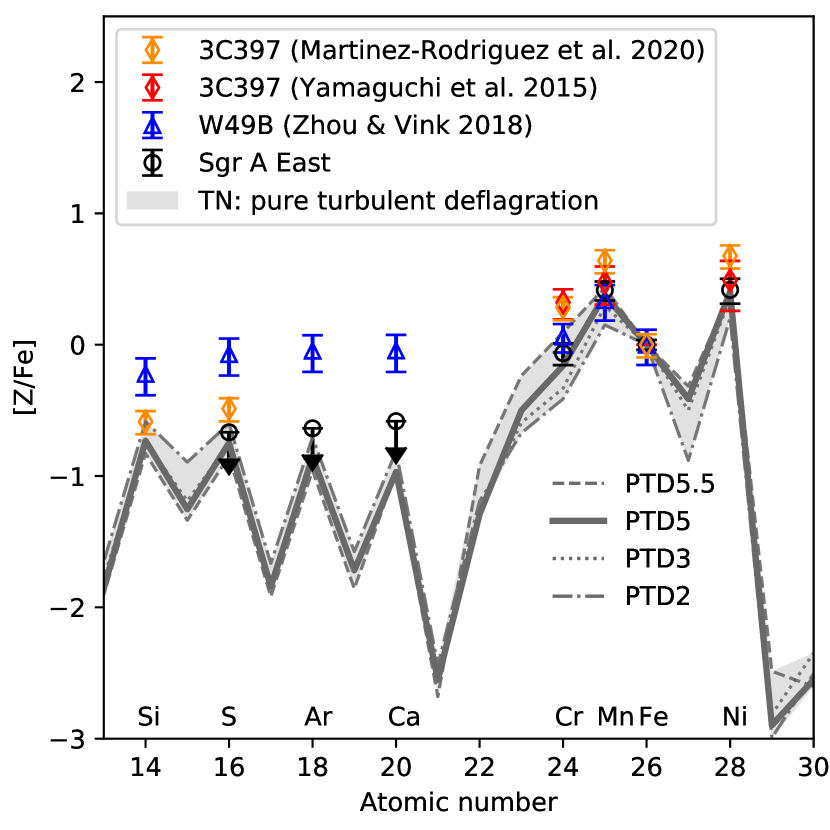
Figure 7: Comparison between the observed logarithmic abundance ratios (relative to Fe) for 3C 397, W49B, and Sgr A East and the PTD models by Leung & Nomoto (2020a). We adopted a 20% systematic error for the ratios from Martínez-Rodríguez et al. (2020), which have very small statistical errors.

Figure 7 compares the logarithmic abundance ratios between Sgr A East and 3C 397 and W49B over the PTD models. It shows that Sgr A East does not have the same abundance pattern as 3C 397 and W49B.

Sgr A East has a significantly lower [Cr/Fe] than 3C 397. The [Cr/Fe] value in 3C 397 is $0.32^{+0.10}_{-0.13}$ (1$\sigma$ error) according to Yamaguchi et al. (2015) using 69 ks of Suzaku data. The value is refined to $0.28^{+0.05}_{-0.09}$ (90% error) in a recent study by Martínez-Rodríguez et al. (2020) using 172 ks of Suzaku data. In contrast, Sgr A East has a sub- or near-solar [Cr/Fe]$=-0.065^{+0.075}_{-0.091}$. The [Mn/Fe] and [Ni/Fe] ratios in Sgr A East are similar to the 3C 397 values determined by Yamaguchi et al. (2015), but are smaller than that obtained by Martínez-Rodríguez et al. (2020).

Unlike Sgr A East, 3C 397 has revealed high IME abundances. Previous studies of 3C 397 gave mass ratios $M_{\rm Ca}/M_{\rm S}=0.213^{+0.021}_{-0.034}$ and $M_{\rm Ar}/M_{\rm S}=0.214^{+0.030}_{-0.026}$, respectively (90% confidence range; Safi-Harb et al., 2005; Martínez-Rodríguez et al., 2017). The recently updated abundance ratios gave $M_{\rm Ca}/M_{\rm S}=0.56^{+0.10}_{-0.15}$ and $M_{\rm Ar}/M_{\rm S}=0.40^{+0.05}_{-0.07}$ (90% confidence range, Martínez-Rodríguez et al., 2020). These new ratios are significantly larger than that predicted by our PTD models ($M_{\rm Ca}/M_{\rm S}=0.12$–0.16 and $M_{\rm Ar}/M_{\rm S}=0.17$–0.18), while the old ratios are only slightly larger than the PTD results. Due to the large discrepancy of the ratios between studies, Figure 7 does not show [Ca/Fe] and [Ar/Fe] ratios for 3C 397. Moreover, the [S/Fe] ratio in 3C 397 (considering a 20% systematic error) is slightly larger than that of Sgr A East.

The progenitor of 3C 397 has been suggested to be a high-metallicity ($Z\sim 5Z_{\odot}$), high-density Chandrasekhar-mass WD, which reproduces the large Mn/Fe and Ni/Fe ratios through a DDT explosion (Yamaguchi et al., 2015; Leung & Nomoto, 2018). Nevertheless, Dave et al. (2017) proposed another solution. In addition to the high-Z, high-$\rho$ DDT models, they found that a PTD explosion of a low central density ($\sim 2\times 10^{9}\,{\rm g}\,{\rm cm}^{-3}$) WD could also reproduce the IGE masses in 3C 397 (see also Leung & Nomoto, 2018). Our PTD models with central densities of 2.0–$5.5\times 10^{9}~{}\,{\rm g}\,{\rm cm}^{-3}$ cannot describe the high [Cr/Fe], [Ca/S], and [Ar/S] in 3C 397. The high-density PTD model N100Hdef in Fink et al. (2014) gives [Cr/Fe]$=0.19$, and thus may marginally explain the high [Cr/Fe] ratio, but it is still difficult to describe the oversolar [Ca/S] and [Ar/S] ratios.

W49B has been proposed as a remnant from a DDT explosion, given its abundance pattern and the large observed IGE masses according to spatially resolved spectroscopic analysis (Zhou & Vink, 2018; Siegel et al., 2020). Figure 7 shows that W49B produces too-large IME/Fe ratios compared to Sgr A East, although the [Cr/Fe] and [Mn/Fe] values are similar to that of Sgr A East.

Some disputes remain on the explosion mechanisms of W49B (Sun & Chen, 2020; Sato et al., 2020a). One major dispute was from the inconsistent metal masses obtained in different studies, although the abundance ratios are more or less consistent (Sun & Chen, 2020; Siegel et al., 2020). When considering low IGE masses, the abundance pattern of W49B (except the high Mn abundance) might also be explained with a core-collapse SNR. We stress that Sgr A East’s IME/Fe, Mn/Fe, and Ni/Fe ratios eliminate core-collapse origins (see Figure 4). In the Appendix (section B), we elaborate that the metal masses for Sgr A East have large uncertainties (over one order of magnitude) and should not be used to distinguish the explosion mechanisms. The main reason is that the derived metal masses are sensitive to the assumed three-dimensional gas geometry and ejecta–ISM mixing, which we do not clearly know. This issue also applies to W49B’s metal masses when analyzing the global spectrum. In the ejecta–ISM mixed case, the metal masses $M_{\rm X}$ were derived mainly using two parameters: the fitted emission measure $EM$ and the filling factor of the gas in the volume $f$ ($M_{\rm X}\propto\sqrt{EMf}$). Consequently, an accurate mass calculation needs a good understanding of $f$. Sun & Chen (2020) fitted the global spectrum using a three-component model and obtained a very small ejecta filling factor $f_{\rm ej}=6.4\%$ and a low Fe mass ($6.0\pm 0.6\times 10^{-2}~{}M_{\odot}$), too small for a Type Ia SN. In contrast, Zhou & Vink (2018) show that the gas in W49B is highly inhomogeneous and obtained a spatially varied $f_{\rm ej}$ with a mean value of $\sim 40\%$. They obtained significantly larger IGE masses ($M({\rm Fe})=0.3\pm 0.1~{}M_{\odot}$). Moreover, the existence of pure ejecta would significantly enhance the metal masses with the same $EM$ and cause extra uncertainties (Park et al., 2005; Greco et al., 2020). Considering the difficulty of obtaining ccurate measurements of the metal masses using a global spectrum and current low-energy-resolution CCD spectra (Greco et al., 2020), a good way is to lean on the abundance/mass ratios, which are less affected by the geometry and pure-ejecta assumptions.

The comparisons in Figures 4– 7 demonstrate the importance of using a large set of element ratios to constrain the SN models. Using only three IGEs (e.g., Mn/Fe or Ni/Fe ratios alone) is insufficient to distinguish PTD and DDT origins in some cases. Sgr A East has a Chandrasekhar-mass WD progenitor, but with a different explosion mechanism from 3C 397 and W49B. The differences among Sgr A East, 3C 397, and W49B provide observational evidence that there is a diversity of thermonuclear SNRs from Chandrasekhar-mass WDs, and they shows that this diversity could be probed by X-ray spectroscopy.

5 Conclusion

We have performed an X-ray spectroscopic study of SNR Sgr A East using 3 Ms of Chandra data. The metal pattern of Sgr A East can be well explained with a pure turbulent deflagration (PTD) explosion of a Chandrasekhar-mass WD, a leading mechanism for producing Type Iax SNe. Sgr A East increases the diversity of the known thermonuclear SNRs and provides a valuable target for the study of Type Iax SNe.

We are aware that our interpretation of Sgr A East’s progenitor highly depends on the existing SN nucleosynthesis models. Model development is important for bringing broader possibilities for a comparison with observations, although the models used in our paper have already covered a wide parameter space. On the other hand, a better understanding of the SN ejecta masses and spatial distribution also help to constrain SN explosion mechanisms. Next-generation X-ray spectrometers with a high spectral resolution will provide crucial insight into the ejecta composition and masses in not only Sgr A East but also other SNRs.

Our main results are summarized as follows:

1. The Chandra ACIS-S spectrum of Sgr A East shows clear emission lines of the S, Ar, Ca, Cr, Mn, Fe, and Ni. The strong Fe He$\alpha$ and Ly$\alpha$ lines have been resolved. The abundances relative to the solar values and the 90% uncertainties of S, Ar, Ca, Cr, Mn, Fe, and Ni elements are $1.4\pm 0.2$, $1.5\pm 0.2$, $1.7\pm 0.1$, $5.6\pm 1.0$, $16.9\pm 2.6$, $6.5\pm 0.4$, and $17.0\pm 3.5$, respectively.

2. A two-temperature plasma model is needed to fit the 2–8 keV spectrum. We found that the best-fit model is an absorbed two-temperature (near-)CIE model with the cool and hot component abundances tied together, consistent with that suggested in previous Chandra and XMM-Newton studies (Park et al., 2005; Sakano et al., 2004). This model suggests that the S–Ni elements between the cool and hot components are well mixed. The two components have temperatures of $\sim 1.2$ keV and $\sim 4.3$ keV, respectively. The foreground absorption is $\sim 2.1\times 10^{23}~{}\,{\rm cm}^{-2}$.

3. Sgr A East shows a low ratio of IMEs to Fe and large Mn/Fe and Ni/Fe ratios. This abundance pattern does not accord with core-collapse SN models (Sukhbold et al., 2016) or normal Type Ia SN models for sub-Chandrasekhar WDs (due to the high Mn/Fe ratio) or DDT of Chandrasekhar-mass WDs with DDT explosions (models from Leung & Nomoto, 2018; Seitenzahl et al., 2013a).

4. The metal composition unveils that Sgr A East originated from a PTD explosion of a Chandrasekhar-mass WD (Leung & Nomoto, 2020a; Fink et al., 2014), a popular mechanism for Type Iax SNe. Sgr A East is thus likely the first identified Type Iax SNR and provides the nearest target for studying this peculiar class of SNe.

5. The existence of a significant amount of dust in Sgr A East (Lau et al., 2015), together with the low ejecta velocity and large C (also O and Fe) production predicted in the best-fit PTD5 models, implies that Type Iax SNe could be potential dust factories. This speculation needs future tests from modelings and observations.

6. Sgr A East shows an abundance pattern distinguished from 3C397 and W49B, which were claimed to result from DDT Chandrasekhar-mass WD explosions (with disputes). The X-ray spectroscopy of SNRs provides observational evidence that there are diverse explosion channels for Chandrasekhar-mass WDs.

Appendix A Spectral fit in small-scale regions

In order to check if the abundance pattern significantly varies across the SNR and if it influences our conclusion on the origin of Sgr A East, we extracted spectra from three small-scale regions (“north,” “middle,” and “south”) as shown in Figure 8. Similar to the global spectrum, the spectra from the three regions can be described using a two-temperature model (see Table 3). The temperature of the cool component and the abundances of IMEs are consistent with the global spectrum, while the absorption column density $N_{\rm H}$ and Fe abundances are increased toward the south. The hot-component emission mainly arises from the regions “middle” and “south,” where the best-fit abundances are closest to those from the global spectrum.

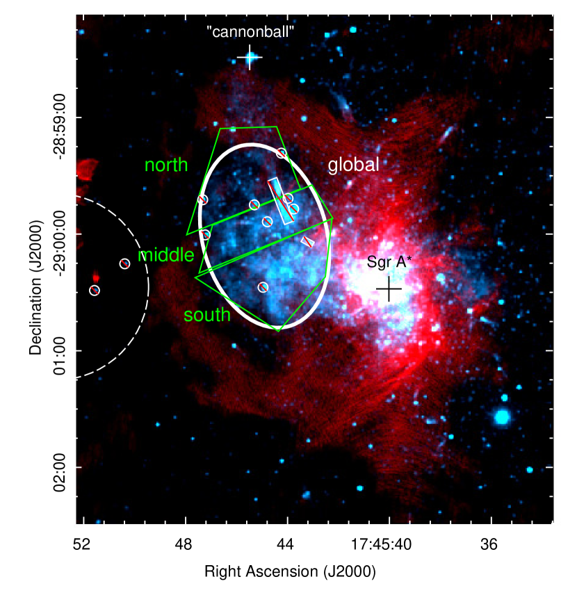
Figure 8: Composite image the same as Figure 1, overlaid with three additional regions for spectral extraction. The spectral fit results are shown in Table 3.

Table 3: Best-fit results for three individual regions with 90% uncertainties

Region	North	Middle	South
$\chi_{\nu}^{2}$/dof	1.20/329	1.20/353	1.19/382
$N_{\rm H}(10^{23}$ cm${}^{-2})$	$1.88\pm 1.0$	$1.97\pm 0.07$	$2.30\pm 0.06$
$kT_{\rm c}$ (keV)	$1.12\pm 0.07$	$1.14\pm 0.05$	$1.21\pm 0.05$
$kT_{\rm h}$ (keV)	$7.4^{+2.5}_{-1.5}$	$4.5\pm 0.4$	$3.9\pm 0.3$
$norm_{\rm c}(\times 10^{-2})$	$1.1\pm 0.3$	$1.5\pm 0.2$	$2.4\pm 0.2$
$norm_{\rm h}(\times 10^{-3})$	$0.4\pm 0.1$	$5.9\pm 0.1$	$1.1\pm 0.2$
S	$1.8\pm 0.4$	$1.4\pm 0.3$	$1.2\pm 0.3$
Ar	$1.9\pm 0.4$	$1.5\pm 0.3$	$1.5\pm 0.3$
Ca	$1.6\pm 0.3$	$1.9\pm 0.2$	$1.7\pm 0.2$
Cr	$4.3\pm 3.2$	$7.0\pm 2.0$	$5.1\pm 1.3$
Mn	$15\pm 9$	$12.6\pm 4.7$	$18.7\pm 3.5$
Fe	$2.4\pm 0.5$	$5.3\pm 0.6$	$8.3\pm 0.6$
Ni	$19\pm 12$	$13.6\pm 5.5$	$20.3\pm 4.9$

The thermonuclear origin of Sgr A East is still favored for these smaller regions, as indicated by the large Mn/Fe abundance ratios (2–6) and the high IGE/IME ratios. PTD remains the best explanation for the individual regions. The Fe abundance in the northern region is lower, indicating less Fe or a stronger mixing with the ambient medium. The other IGE abundances in the northern region have large uncertainties.

Moreover, we note that the single-component models $vvrnei$ and $bvvrnei$ for the global spectrum in the 5–8 keV band (see Table 3) also suggest high Mn/Fe and Cr/Fe ratios typical for the PTD models, although the single-component model does not give a good fit as the two-temperature model.

Appendix B Gas parameters and SNR properties

The best-fit two-temperature model implies that the plasma in Sgr A East is a mixture of cool and hot gas. Assuming that the X-ray bremsstrahlung emission is from the plasma with near-solar metallicity, the gas densities in the cool and hot phases are derived as $n_{\rm H}^{\rm c}=11.2\pm 1.5f^{-1/2}$ cm^-3 and $n_{\rm H}^{\rm h}=3.1\pm 0.7f^{-1/2}$ cm^-3, respectively, where $f$ is the filling factor of the observed X-ray-emitting gas in the whole volume. The densities are calculated using the best-fit emission measures (proportional to the parameter $norm$) and an assumed a prolate ellipsoid geometry of the X-ray-emitting plasma (short half-axis of $32^{\prime\prime}$ and long half-axis of $48^{\prime\prime}$, as shown in Figure 8). The cool and hot gas phases are considered to fill $f$ of the whole volume and in pressure equilibrium, $n_{\rm H}^{\rm c}kT_{\rm c}$=$n_{\rm H}^{\rm h}kT_{\rm h}$. This gives the filling factor of the cool phase as $f_{\rm c}=0.65\pm 0.15f$.

We also obtain the gas mass to be $3.6\pm 0.4f^{1/2}~{}M_{\odot}$ in the cool phase and $0.55\pm 0.11f^{1/2}~{}M_{\odot}$ in the hot phase. Therefore, assuming that the ejecta and ISM are well mixed, the total mass of the X-ray-emitting gas is $4.2\pm 0.4f^{1/2}~{}M_{\odot}$. Then the total observed IGE masses are obtained as $M$(Cr)$=3.2\pm 0.8\times 10^{-4}f^{1/2}~{}M_{\odot}$, $M$(Mn)$=7.3\pm 1.4\times 10^{-4}f^{1/2}~{}M_{\odot}$, $M$(Fe)$=3.0\pm 0.4\times 10^{-2}f^{1/2}~{}M_{\odot}$, and $M$(Ni)$=4.8\pm 1.2\times 10^{-3}f^{1/2}~{}M_{\odot}$. These values are around one order of magnitude smaller than the values predicted in the best-fit PTD5 model with centered flame structures. Nevertheless, we note the possibility that the X-ray emission might be partly from the pure SN ejecta (Park et al., 2005). In this case, the metal masses could be greatly enhanced with the same X-ray emission measure.

Pure-Fe ejecta has been found in the young SNR Cassiopeia A (Hwang & Laming, 2012). It has also been speculated that pure metal exists in the middle-age SNR W49B (Vink, 2012; Zhou & Vink, 2018; Greco et al., 2020). Similar to Sgr A East, W49B is also a Fe-rich, mixed-morphology SNR interacting with dense ambient medium (e.g., Keohane et al., 2007; Miceli et al., 2010; Zhu et al., 2014). In the pure ejecta case, the Bremsstrahlung emission measure is expressed as $EM=\sum n_{e}n_{i}Z_{i}^{2}V$, where $n_{e}$, $n_{i}$, $Z_{i}$ and $V$ are the electron density, ion density, charge on the ion, and the ejecta volume. Consequently, the IGE masses could be much larger than the values derived above. The degeneracy between the best-fit abundances and emission measure leads to big uncertainties in mass estimates. Recently, Greco et al. (2020) pointed out that a bright radiative recombining continuum shows up when the plasma is made of pure-metal ejecta. This introduces further difficulties in distinguishing recombining plasma and pure ejecta plasma using the current CCD detectors.

Assuming that most Fe ions are He-like and the ejecta have a filling factor $f$, we obtained the Fe densities in the cool and hot components to be $0.10\pm 0.01f^{-1/2}$ cm^-3 and $0.029\pm 0.006f^{-1/2}$ cm^-3, respectively. The total Fe mass in this extreme case is thus $1.6\pm 0.3f^{1/2}M_{\odot}$. This is an upper limit of Fe mass, as the filling factor $f$ of pure ejecta cannot be larger than 1 and the ejecta should be mixed with some shocked ISM. Moreover, the Fe mass estimated here highly depends on the assumption of the three-dimensional morphology of the X-ray-emitting region. We assumed a larger volume, resulting in a larger Fe mass than that derived in Park et al. (2005). Therefore, the observed IGE masses have large uncertainties, although their abundance ratios are not affected by the mixing problem for Sgr A East.

One explanation for the two-temperature gas is that the cool and hot components correspond to the gas shocked by the blast waves and reverse shock, respectively. However, it is hard to explain why the abundances of the gas shocked by the blast wave are also rich in IGEs. In an alternative explanation, the cool component corresponds to the denser clumps, while the hot component is from the intercloud medium. Both components are heated by the reverse shock. As the X-ray photons below 2 keV are strongly absorbed, we do not know if there is a third component colder than 1 keV.

Sgr A East is among the smallest SNRs, with a size of 5.5 pc $\times 7.8$ pc (Zhao et al., 2016), around half the size of W49B with an age of 5–6 kyr (Zhou & Vink, 2018; Sun & Chen, 2020). This indicates that Sgr A East is either young, evolving in a dense medium, or has smaller explosion energy. Using Sedov-Taylor self-similar solution (Sedov, 1959; Taylor, 1950; Ostriker & McKee, 1988), we find the explosion energy is $E_{0}=(1/4\xi)(1.4n_{0}m_{\rm H})R_{\rm s}^{5}t_{\rm s}^{-2}\sim 3.2\times 10^{50}(n_{0}/10~{}{\rm cm}^{-3})(R_{\rm s}/3.3~{}{\rm pc})^{5}(t/{\rm 2~{}kyr})^{-2}$ erg, where $\xi=2.026$ and $n_{0}$ is the mean ambient density, $R_{\rm s}$ is the radius of the SNR (the major and minor axes of the SNR are 2.75 pc and 3.9 pc, respectively), and $t$ is the SNR age.

There is no consensus on the age of Sgr A East. Hydrodynamic simulations favored an early stage of the SNR ($\lesssim 2$ kyr, Rockefeller et al., 2005; Fryer et al., 2006). In contrast, a few earlier X-ray studies suggested a large age for Sgr A East, in order to explain the (near-)CIE state of the plasma or to establish a presumed connection with the “cannonball” neutron star (5000–$10^{4}$ yr, Maeda et al., 2002; Sakano et al., 2004). We note that the large ionization timescale of Sgr A East’s plasma does not necessarily support a large age. The ionization timescale $\tau$ of X-ray plasma has been used to infer the SNR age $t=\tau/n_{e}$, based on an assumption of a constant electron density and simplest ionization history. If the spectrum is not dominated by the pure ejecta, our spectral fit gives a 1$\sigma$ shock age of 2–$3f^{1/2}$ kyr for the cool component, consistent with the young stage of Sgr A East. The hot component is in CIE, but the origin of this CIE state cannot be simply explained with a large shock age. Unlike the cool component, the electron temperature of the hot component varies by a factor of two across the SNR, as shown in previous studies (Park et al., 2005; Sakano et al., 2004) and in Table 3. Such a large temperature gradient has also been found in the hot component of W49B, which has overionized plasma (0.6–2.2 keV, Miceli et al., 2010; Lopez et al., 2013a; Zhou & Vink, 2018; Yamaguchi et al., 2018). The variation of electron temperature and CIE state could result from rapid cooling processes such as thermal conduction with cold gas or adiabatic cooling. Moreover, a high ionization stage of ions could be caused by the X-ray photoionization from past flares of Sgr A* (Ono et al., 2019).

Sgr A East  is impacting a dense molecular shell in the east (Mezger et al., 1996; Yusef-Zadeh et al., 2000), which was unlikely to be swept up by the SNR itself, as it would require a too-energetic SN explosion ($E_{0}\sim 4\times 10^{52}$ erg Mezger et al., 1989). We have shown that Sgr A East originates from a PTD WD explosion, which cannot have an ultrahigh explosion energy. The density of the X-ray-emitting gas is $\lesssim 10$ cm${}^{-3}f^{-1/2}$, a few orders of magnitude smaller than that of a dense molecular cloud. Therefore, our study supports that Sgr A East was evolving in a relatively low-density medium until its shocks impacted the preexisting molecular shell (Serabyn et al., 1992). A possible source that shaped the molecular shell is the winds of irrelevant massive stars in the SNR interior. Another source of the winds could be strong accretion outflows from the progenitor WD binary system prior to the SN explosion (Hachisu et al., 1996). Wind-blown molecular bubbles have been reported for Type Ia SNR Tycho (Zhou et al., 2016; Chen et al., 2017) and N103B (Sano et al., 2018). Dense wind bubbles have also been found in Type Ia SNR candidates RCW 86 (Williams et al., 2011) and W49B (Keohane et al., 2007; Zhou & Vink, 2018).

Appendix C Numerical simulations of Type Ia SN models

We have the formalism presented in detailed parameter surveys for two-dimensional Type Ia SNe of near-Chandrasekhar-mass WD models with or without deflagration-detonation transition (Leung et al., 2015; Leung & Nomoto, 2018, 2020a) and for sub-Chandrasekhar-mass WD (Leung & Nomoto, 2020b). We use the three-step nuclear reactions (Townsley et al., 2007; Calder et al., 2007) with parameterized timescales for the carbon deflagration and detonation. The chemical composition is described by a seven-isotope network (Timmes et al., 2000), including ⁴He, ¹²C, ¹⁶O, ²⁰Ne, ²⁴Mg, ²⁸Si, and ⁵⁶Ni. To capture the deflagration and detonation, we use the level-set method (Osher & Sethian, 1988; Reinecke et al., 1999). The prescription of the sub-grid-scale turbulence model (Niemeyer & Hillebrandt, 1995; Schmidt et al., 2006) is specific for the turbulent deflagration with a specific turbulent flame formula (Hicks, 2015). To determine whether the DDT occurs, we use the criteria by comparing the local size of the eddy motion with the flame width (Golombek & Niemeyer, 2005). For the sub-Chandrasekhar-mass models, where no deflagration takes place, we check the trigger of the carbon detonation by using the local density and temperature (Fink et al., 2014). We use the tracer particle scheme (Travaglio et al., 2004; Seitenzahl et al., 2010) to record the thermodynamical history of the star. The tracers are designed to be massless and are passively advected by the fluid motion. They record the density and temperature experienced according to the local quantities from the Eulerian meshes. To compute the nucleosynthesis yield, we choose a large 495-isotope network (Timmes, 1999) which includes isotopes from ¹H to ⁹¹Tc, and we apply this network to the thermodynamical trajectories of all the tracer particles.

For the near-Chandrasekhar-mass WD models, the simulations are done by first setting up a C+O WD with a given central density $\rho_{c}$ (metallicity $Z=Z_{\odot}$ in this work); this corresponds to a specific WD mass $M$. Then we put in the initial nuclear deflagration by hand at the center or at off-center. We allow the deflagration to propagate and interact with the fluid motion. For the models with DDT, we further set the code to check if the flame front satisfies the transition criteria. If this is achieved, we put in by hand carbon detonation bubbles and allow them to propagate independently with the carbon deflagration waves. We carry out the simulation until the star develops into homologous expansion and becomes sufficiently cold such that no major exothermic nuclear reactions continue.

For the sub-Chandrasekhar-mass WD models, the simulations are done by first setting a C+O WD with a helium envelope. The central density and the transition density from the C$+$O core to the He envelope are chosen such that the total mass $M$ and the He-envelope $M_{\rm He}$ mass are as required. After that, we put in the initial detonation by hand in the He envelope and start the simulation. The local thermodynamical condition in the C+O core is checked to see if the second detonation can be triggered by the shock wave interactions generated by the He detonation. When the condition is met, a carbon detonation bubble is put in by hand, and we let the carbon detonation and helium detonation propagate independently until the star is totally disrupted and reaches homologous expansion.

Table 4 shows the basic parameters of the thermonuclear SN models used in Figure 4, where the original names of the models are listed. We also summarize the nucleosynthesis yields of the thermonuclear models in Table 5 and Table 6.

Table 4: Basic parameters and model conversion for thermonuclear SN models.

Model	Explosion Type	Ejecta Mass	Remnant Mass	56Ni	44Ti	Model in Reference
		($M_{\odot}$)	($M_{\odot}$)	($M_{\odot}$)	($M_{\odot}$)
DDT2	DDT	1.35		0.70	3.28e-5	200-1-c3-1
DDT3		1.37		0.63	2.47e-5	300-1-c3-1
DDT5		1.38		0.60	2.29e-5	500-1-c3-1
DDT5.5		1.38		0.75	2.76e-5	550-1-c3-1
Bubble ($1.1M_{\odot}$)	DD	1.10		0.61	5.14e-4	110-100-2-50
Ring ($1.1M_{\odot}$)		1.10		0.68	5.99e-4	110-050-2-B50
Sphere ($1.0M_{\odot}$)		1.00		0.60	2.64e-4	100-050-2-S50
Sphere ($0.9M_{\odot}$)		0.90		0.0155	3.27e-5	090-050-2-S50
PTD2	PTD	1.18	0.17	0.24	1.64e-6	200-135-1-c3-1
PTD3		1.26	0.11	0.34	1.79e-6	300-137-1-c3-1
PTD5		1.29	0.09	0.32	1.75e-6	500-138-1-c3-1
PTD5.5		1.30	0.08	0.31	1.51e-6	550-138-1-c3-1

• “DD,” “DDT,” and “PTD” correspond to the double detonation model (Leung & Nomoto, 2020b), turbulent deflagration model with deflagration-detonation transition (Leung & Nomoto, 2018), and pure turbulent deflagration model, respectively (Leung & Nomoto, 2020a).

Table 5: Nucleosynthesis yields in unit of $M_{\odot}$ for the DDT and DD models (Type Ia, Leung & Nomoto, 2018, 2020b).

Element	DDT2	DDT3	DDT5	DDT5.5	Bubble	Ring	Sphere
C	$1.4\times 10^{-3}$	$1.7\times 10^{-3}$	$5.82\times 10^{-4}$	$4.38\times 10^{-6}$	$3.35\times 10^{-3}$	$4.2\times 10^{-3}$	$1.15\times 10^{-3}$
N	$1.72\times 10^{-10}$	$2.34\times 10^{-10}$	$5.2\times 10^{-10}$	$5.60\times 10^{-11}$	$3.90\times 10^{-8}$	$1.18\times 10^{-7}$	$1.84\times 10^{-8}$
O	$3.83\times 10^{-2}$	$5.69\times 10^{-2}$	$4.90\times 10^{-2}$	$1.29\times 10^{-2}$	$1.17\times 10^{-1}$	$1.2\times 10^{-1}$	$6.64\times 10^{-2}$
F	$3.18\times 10^{-14}$	$1.38\times 10^{-13}$	$8.34\times 10^{-13}$	$1.59\times 10^{-16}$	$3.28\times 10^{-11}$	$6.80\times 10^{-11}$	$2.39\times 10^{-11}$
Ne	$1.66\times 10^{-4}$	$1.81\times 10^{-4}$	$6.77\times 10^{-4}$	$2.15\times 10^{-6}$	$4.9\times 10^{-3}$	$4.81\times 10^{-3}$	$1.15\times 10^{-3}$
Na	$5.38\times 10^{-7}$	$8.9\times 10^{-7}$	$2.0\times 10^{-6}$	$4.57\times 10^{-8}$	$1.47\times 10^{-5}$	$2.10\times 10^{-5}$	$8.39\times 10^{-6}$
Mg	$8.54\times 10^{-4}$	$1.11\times 10^{-3}$	$1.24\times 10^{-3}$	$3.42\times 10^{-4}$	$8.36\times 10^{-3}$	$8.75\times 10^{-3}$	$1.32\times 10^{-3}$
Al	$7.17\times 10^{-5}$	$9.14\times 10^{-5}$	$9.18\times 10^{-5}$	$2.87\times 10^{-5}$	$6.50\times 10^{-4}$	$7.17\times 10^{-4}$	$1.14\times 10^{-4}$
Si	$2.21\times 10^{-1}$	$2.35\times 10^{-1}$	$2.9\times 10^{-1}$	$1.6\times 10^{-1}$	$1.37\times 10^{-1}$	$1.13\times 10^{-1}$	$1.25\times 10^{-1}$
P	$1.33\times 10^{-4}$	$1.92\times 10^{-4}$	$1.65\times 10^{-4}$	$4.17\times 10^{-5}$	$3.97\times 10^{-4}$	$3.54\times 10^{-4}$	$1.53\times 10^{-4}$
S	$1.20\times 10^{-1}$	$1.25\times 10^{-1}$	$1.11\times 10^{-1}$	$6.64\times 10^{-2}$	$6.38\times 10^{-2}$	$5.13\times 10^{-2}$	$6.77\times 10^{-2}$
Cl	$1.50\times 10^{-4}$	$2.4\times 10^{-4}$	$1.82\times 10^{-4}$	$3.78\times 10^{-5}$	$1.84\times 10^{-4}$	$1.54\times 10^{-4}$	$1.29\times 10^{-4}$
Ar	$2.32\times 10^{-2}$	$2.41\times 10^{-2}$	$2.14\times 10^{-2}$	$1.47\times 10^{-2}$	$1.10\times 10^{-2}$	$8.57\times 10^{-3}$	$1.29\times 10^{-2}$
K	$1.44\times 10^{-4}$	$1.89\times 10^{-4}$	$1.75\times 10^{-4}$	$3.54\times 10^{-5}$	$1.15\times 10^{-4}$	$9.9\times 10^{-5}$	$9.82\times 10^{-5}$
Ca	$1.83\times 10^{-2}$	$1.80\times 10^{-2}$	$1.60\times 10^{-2}$	$1.43\times 10^{-2}$	$9.7\times 10^{-3}$	$7.52\times 10^{-3}$	$1.7\times 10^{-2}$
Sc	$5.21\times 10^{-7}$	$6.5\times 10^{-7}$	$5.71\times 10^{-7}$	$2.18\times 10^{-7}$	$1.67\times 10^{-6}$	$7.81\times 10^{-7}$	$3.77\times 10^{-7}$
Ti	$4.50\times 10^{-4}$	$4.9\times 10^{-4}$	$9.16\times 10^{-4}$	$1.53\times 10^{-3}$	$5.5\times 10^{-3}$	$2.72\times 10^{-3}$	$7.64\times 10^{-4}$
V	$8.47\times 10^{-5}$	$9.47\times 10^{-5}$	$2.88\times 10^{-4}$	$3.59\times 10^{-4}$	$5.90\times 10^{-4}$	$2.81\times 10^{-4}$	$7.62\times 10^{-5}$
Cr	$7.19\times 10^{-3}$	$9.58\times 10^{-3}$	$2.22\times 10^{-2}$	$2.78\times 10^{-2}$	$1.68\times 10^{-2}$	$3.7\times 10^{-3}$	$3.29\times 10^{-3}$
Mn	$8.70\times 10^{-3}$	$1.3\times 10^{-2}$	$1.34\times 10^{-2}$	$1.43\times 10^{-2}$	$2.28\times 10^{-3}$	$9.15\times 10^{-4}$	$1.32\times 10^{-3}$
Fe	$8.23\times 10^{-1}$	$7.99\times 10^{-1}$	$8.37\times 10^{-1}$	$10.7\times 10^{-1}$	$6.40\times 10^{-1}$	$7.8\times 10^{-1}$	$6.25\times 10^{-1}$
Co	$8.22\times 10^{-4}$	$8.85\times 10^{-4}$	$1.25\times 10^{-3}$	$1.47\times 10^{-3}$	$7.19\times 10^{-4}$	$6.17\times 10^{-4}$	$5.27\times 10^{-4}$
Ni	$7.31\times 10^{-2}$	$7.70\times 10^{-2}$	$8.69\times 10^{-2}$	$9.84\times 10^{-2}$	$4.37\times 10^{-2}$	$3.91\times 10^{-2}$	$3.31\times 10^{-2}$
Cu	$5.83\times 10^{-6}$	$4.12\times 10^{-6}$	$7.29\times 10^{-6}$	$1.7\times 10^{-5}$	$2.32\times 10^{-5}$	$5.73\times 10^{-6}$	$1.1\times 10^{-5}$
Zn	$6.99\times 10^{-5}$	$4.53\times 10^{-5}$	$4.76\times 10^{-5}$	$6.87\times 10^{-5}$	$1.79\times 10^{-4}$	$3.62\times 10^{-5}$	$5.19\times 10^{-5}$

Table 6: Nucleosynshesis yields in unit of $M_{\odot}$ for the PTD models (Type Iax, Leung & Nomoto, 2020a)

Element	PTD2	PTD3	PTD5	PTD5.5
C	$3.81\times 10^{-1}$	$3.21\times 10^{-1}$	$3.14\times 10^{-1}$	$3.14\times 10^{-1}$
N	$5.29\times 10^{-9}$	$7.29\times 10^{-9}$	$6.67\times 10^{-9}$	$6.15\times 10^{-9}$
O	$4.8\times 10^{-1}$	$3.54\times 10^{-1}$	$3.44\times 10^{-1}$	$3.40\times 10^{-1}$
F	$1.52\times 10^{-11}$	$1.81\times 10^{-11}$	$1.75\times 10^{-11}$	$1.65\times 10^{-11}$
Ne	$1.86\times 10^{-2}$	$1.63\times 10^{-2}$	$1.59\times 10^{-2}$	$1.59\times 10^{-2}$
Na	$9.76\times 10^{-6}$	$1.5\times 10^{-5}$	$1.5\times 10^{-5}$	$1.2\times 10^{-5}$
Mg	$3.63\times 10^{-3}$	$4.5\times 10^{-3}$	$3.80\times 10^{-3}$	$3.49\times 10^{-3}$
Al	$2.67\times 10^{-4}$	$3.1\times 10^{-4}$	$2.78\times 10^{-4}$	$2.59\times 10^{-4}$
Si	$3.72\times 10^{-2}$	$4.10\times 10^{-2}$	$4.45\times 10^{-2}$	$3.69\times 10^{-2}$
P	$1.6\times 10^{-4}$	$1.27\times 10^{-4}$	$1.17\times 10^{-4}$	$1.0\times 10^{-4}$
S	$1.67\times 10^{-2}$	$1.82\times 10^{-2}$	$1.99\times 10^{-2}$	$1.64\times 10^{-2}$
Cl	$3.81\times 10^{-5}$	$4.40\times 10^{-5}$	$4.24\times 10^{-5}$	$3.71\times 10^{-5}$
Ar	$2.83\times 10^{-3}$	$3.10\times 10^{-3}$	$3.35\times 10^{-3}$	$2.75\times 10^{-3}$
K	$1.75\times 10^{-5}$	$1.93\times 10^{-5}$	$2.11\times 10^{-5}$	$1.59\times 10^{-5}$
Ca	$2.13\times 10^{-3}$	$2.35\times 10^{-3}$	$2.48\times 10^{-3}$	$2.6\times 10^{-3}$
Sc	$3.64\times 10^{-8}$	$4.41\times 10^{-8}$	$4.68\times 10^{-8}$	$3.63\times 10^{-8}$
Ti	$4.31\times 10^{-5}$	$5.60\times 10^{-5}$	$5.73\times 10^{-5}$	$1.4\times 10^{-4}$
V	$1.45\times 10^{-5}$	$2.73\times 10^{-5}$	$3.60\times 10^{-5}$	$6.88\times 10^{-5}$
Cr	$1.38\times 10^{-3}$	$2.61\times 10^{-3}$	$4.14\times 10^{-3}$	$7.72\times 10^{-3}$
Mn	$3.29\times 10^{-3}$	$7.18\times 10^{-3}$	$9.3\times 10^{-3}$	$1.1\times 10^{-2}$
Fe	$2.78\times 10^{-1}$	$4.36\times 10^{-1}$	$4.65\times 10^{-1}$	$4.83\times 10^{-1}$
Co	$1.19\times 10^{-4}$	$4.5\times 10^{-4}$	$5.85\times 10^{-4}$	$7.6\times 10^{-4}$
Ni	$2.45\times 10^{-2}$	$5.5\times 10^{-2}$	$6.5\times 10^{-2}$	$6.48\times 10^{-2}$
Cu	$1.57\times 10^{-7}$	$3.72\times 10^{-7}$	$3.28\times 10^{-7}$	$8.78\times 10^{-7}$
Zn	$1.17\times 10^{-6}$	$2.63\times 10^{-6}$	$1.76\times 10^{-6}$	$1.62\times 10^{-6}$

References

- Arnaud (1996) Arnaud, K. A. 1996, in Astronomical Society of the Pacific Conference Series, Vol. 101, Astronomical Data Analysis Software and Systems V, ed. G. H. Jacoby & J. Barnes, 17
- Asplund et al. (2009) Asplund, M., Grevesse, N., Sauval, A. J., & Scott, P. 2009, ARA&A, 47, 481, doi: 10.1146/annurev.astro.46.060407.145222
- Benvenuto et al. (2015) Benvenuto, O. G., Panei, J. A., Nomoto, K., Kitamura, H., & Hachisu, I. 2015, ApJ, 809, L6, doi: 10.1088/2041-8205/809/1/L6
- Branch et al. (2004) Branch, D., Baron, E., Thomas, R. C., et al. 2004, PASP, 116, 903, doi: 10.1086/425081
- Calder et al. (2007) Calder, A. C., Townsley, D. M., Seitenzahl, I. R., et al. 2007, ApJ, 656, 313, doi: 10.1086/510709
- Chen et al. (2017) Chen, X., Xiong, F., & Yang, J. 2017, A&A, 604, A13, doi: 10.1051/0004-6361/201630003
- Dave et al. (2017) Dave, P., Kashyap, R., Fisher, R., et al. 2017, ApJ, 841, 58, doi: 10.3847/1538-4357/aa7134
- Davies et al. (2009) Davies, B., Figer, D. F., Kudritzki, R.-P., et al. 2009, ApJ, 707, 844, doi: 10.1088/0004-637X/707/1/844
- Ekers et al. (1983) Ekers, R. D., van Gorkom, J. H., Schwarz, U. J., & Goss, W. M. 1983, A&A, 122, 143
- Ferrand & Safi-Harb (2012) Ferrand, G., & Safi-Harb, S. 2012, Advances in Space Research, 49, 1313, doi: 10.1016/j.asr.2012.02.004
- Fink et al. (2014) Fink, M., Kromer, M., Seitenzahl, I. R., et al. 2014, MNRAS, 438, 1762, doi: 10.1093/mnras/stt2315
- Foley et al. (2016) Foley, R. J., Jha, S. W., Pan, Y.-C., et al. 2016, MNRAS, 461, 433, doi: 10.1093/mnras/stw1320
- Foley et al. (2013) Foley, R. J., Challis, P. J., Chornock, R., et al. 2013, ApJ, 767, 57, doi: 10.1088/0004-637X/767/1/57
- Foster et al. (2012) Foster, A. R., Ji, L., Smith, R. K., & Brickhouse, N. S. 2012, ApJ, 756, 128, doi: 10.1088/0004-637X/756/2/128
- Fox et al. (2016) Fox, O. D., Johansson, J., Kasliwal, M., et al. 2016, ApJ, 816, L13, doi: 10.3847/2041-8205/816/1/L13
- Fruscione et al. (2006) Fruscione, A., McDowell, J. C., Allen, G. E., et al. 2006, in Society of Photo-Optical Instrumentation Engineers (SPIE) Conference Series, Vol. 6270, Society of Photo-Optical Instrumentation Engineers (SPIE) Conference Series, 62701V, doi: 10.1117/12.671760
- Fryer et al. (2006) Fryer, C. L., Rockefeller, G., Hungerford, A., & Melia, F. 2006, ApJ, 638, 786, doi: 10.1086/498968
- Golombek & Niemeyer (2005) Golombek, I., & Niemeyer, J. C. 2005, A&A, 438, 611, doi: 10.1051/0004-6361:20042402
- Greco et al. (2020) Greco, E., Vink, J., Miceli, M., et al. 2020, arXiv e-prints, arXiv:2004.12924. https://arxiv.org/abs/2004.12924
- Green (2017) Green, D. A. 2017, VizieR Online Data Catalog, 7278
- Hachisu et al. (1996) Hachisu, I., Kato, M., & Nomoto, K. 1996, ApJ, 470, L97, doi: 10.1086/310303
- Hicks (2015) Hicks, E. P. 2015, ApJ, 803, 72, doi: 10.1088/0004-637X/803/2/72
- Hwang & Laming (2012) Hwang, U., & Laming, J. M. 2012, ApJ, 746, 130, doi: 10.1088/0004-637X/746/2/130
- Jha (2017) Jha, S. W. 2017, Type Iax Supernovae, ed. A. W. Alsabti & P. Murdin, 375, doi: 10.1007/978-3-319-21846-5_42
- Jha et al. (2019) Jha, S. W., Maguire, K., & Sullivan, M. 2019, Nature Astronomy, 3, 706, doi: 10.1038/s41550-019-0858-0
- Keohane et al. (2007) Keohane, J. W., Reach, W. T., Rho, J., & Jarrett, T. H. 2007, ApJ, 654, 938, doi: 10.1086/509311
- Koyama et al. (2007) Koyama, K., Uchiyama, H., Hyodo, Y., et al. 2007, PASJ, 59, 237, doi: 10.1093/pasj/59.sp1.S237
- Lau et al. (2015) Lau, R. M., Herter, T. L., Morris, M. R., Li, Z., & Adams, J. D. 2015, Science, 348, 413, doi: 10.1126/science.aaa2208
- Lazendic et al. (2006) Lazendic, J. S., Dewey, D., Schulz, N. S., & Canizares, C. R. 2006, ApJ, 651, 250, doi: 10.1086/507481
- Leung et al. (2015) Leung, S. C., Chu, M. C., & Lin, L. M. 2015, MNRAS, 454, 1238, doi: 10.1093/mnras/stv1923
- Leung & Nomoto (2018) Leung, S.-C., & Nomoto, K. 2018, ApJ, 861, 143, doi: 10.3847/1538-4357/aac2df
- Leung & Nomoto (2020a) —. 2020a, arXiv e-prints, arXiv:2007.08466. https://arxiv.org/abs/2007.08466
- Leung & Nomoto (2020b) —. 2020b, ApJ, 888, 80, doi: 10.3847/1538-4357/ab5c1f
- Li et al. (2011) Li, W., Chornock, R., Leaman, J., et al. 2011, MNRAS, 412, 1473, doi: 10.1111/j.1365-2966.2011.18162.x
- Li et al. (2003) Li, W., Filippenko, A. V., Chornock, R., et al. 2003, PASP, 115, 453, doi: 10.1086/374200
- Long et al. (2014) Long, M., Jordan, George C., I., van Rossum, D. R., et al. 2014, ApJ, 789, 103, doi: 10.1088/0004-637X/789/2/103
- Lopez et al. (2013a) Lopez, L. A., Pearson, S., Ramirez-Ruiz, E., et al. 2013a, ApJ, 777, 145, doi: 10.1088/0004-637X/777/2/145
- Lopez et al. (2013b) Lopez, L. A., Ramirez-Ruiz, E., Castro, D., & Pearson, S. 2013b, ApJ, 764, 50, doi: 10.1088/0004-637X/764/1/50
- Lyman et al. (2013) Lyman, J. D., James, P. A., Perets, H. B., et al. 2013, MNRAS, 434, 527, doi: 10.1093/mnras/stt1038
- Maeda et al. (2002) Maeda, Y., Baganoff, F. K., Feigelson, E. D., et al. 2002, ApJ, 570, 671, doi: 10.1086/339773
- Martínez-Rodríguez et al. (2017) Martínez-Rodríguez, H., Badenes, C., Yamaguchi, H., et al. 2017, ApJ, 843, 35, doi: 10.3847/1538-4357/aa72f8
- Martínez-Rodríguez et al. (2020) Martínez-Rodríguez, H., Lopez, L. A., Auchettl, K., et al. 2020, arXiv e-prints, arXiv:2006.08681. https://arxiv.org/abs/2006.08681
- McCully et al. (2014) McCully, C., Jha, S. W., Foley, R. J., et al. 2014, ApJ, 786, 134, doi: 10.1088/0004-637X/786/2/134
- Mezger et al. (1996) Mezger, P. G., Duschl, W. J., & Zylka, R. 1996, A&A Rev., 7, 289, doi: 10.1007/s001590050007
- Mezger et al. (1989) Mezger, P. G., Zylka, R., Salter, C. J., et al. 1989, A&A, 209, 337
- Miceli et al. (2010) Miceli, M., Bocchino, F., Decourchelle, A., Ballet, J., & Reale, F. 2010, A&A, 514, L2, doi: 10.1051/0004-6361/200913713
- Niemeyer & Hillebrandt (1995) Niemeyer, J. C., & Hillebrandt, W. 1995, ApJ, 452, 769, doi: 10.1086/176345
- Nomoto et al. (2013) Nomoto, K., Kobayashi, C., & Tominaga, N. 2013, ARA&A, 51, 457, doi: 10.1146/annurev-astro-082812-140956
- Nomoto & Leung (2018) Nomoto, K., & Leung, S.-C. 2018, Space Sci. Rev., 214, 67, doi: 10.1007/s11214-018-0499-0
- Nomoto et al. (1976) Nomoto, K., Sugimoto, D., & Neo, S. 1976, Ap&SS, 39, L37, doi: 10.1007/BF00648354
- Nomoto et al. (1984) Nomoto, K., Thielemann, F.-K., & Yokoi, K. 1984, ApJ, 286, 644, doi: 10.1086/162639
- Nozawa et al. (2003) Nozawa, T., Kozasa, T., Umeda, H., Maeda, K., & Nomoto, K. 2003, ApJ, 598, 785, doi: 10.1086/379011
- Nozawa et al. (2011) Nozawa, T., Maeda, K., Kozasa, T., et al. 2011, ApJ, 736, 45, doi: 10.1088/0004-637X/736/1/45
- Nynka et al. (2013) Nynka, M., Hailey, C. J., Mori, K., et al. 2013, ApJ, 778, L31, doi: 10.1088/2041-8205/778/2/L31
- Ono et al. (2019) Ono, A., Uchiyama, H., Yamauchi, S., et al. 2019, PASJ, 71, 52, doi: 10.1093/pasj/psz025
- Osher & Sethian (1988) Osher, S., & Sethian, J. A. 1988, Journal of Computational Physics, 79, 12, doi: 10.1016/0021-9991(88)90002-2
- Ostriker & McKee (1988) Ostriker, J. P., & McKee, C. F. 1988, Rev. Mod. Phys., 60, 1, doi: 10.1103/RevModPhys.60.1
- Park et al. (2005) Park, S., Muno, M. P., Baganoff, F. K., et al. 2005, ApJ, 631, 964, doi: 10.1086/432639
- Raddi et al. (2019) Raddi, R., Hollands, M. A., Koester, D., et al. 2019, MNRAS, 1623, doi: 10.1093/mnras/stz1618
- Reinecke et al. (2002) Reinecke, M., Hillebrandt, W., & Niemeyer, J. C. 2002, A&A, 386, 936, doi: 10.1051/0004-6361:20020323
- Reinecke et al. (1999) Reinecke, M., Hillebrandt, W., Niemeyer, J. C., Klein, R., & Gröbl, A. 1999, A&A, 347, 724. https://arxiv.org/abs/astro-ph/9812119
- Rockefeller et al. (2005) Rockefeller, G., Fryer, C. L., Baganoff, F. K., & Melia, F. 2005, ApJ, 635, L141, doi: 10.1086/499360
- Röpke et al. (2007) Röpke, F. K., Hillebrandt, W., Schmidt, W., et al. 2007, ApJ, 668, 1132, doi: 10.1086/521347
- Rudolph et al. (2006) Rudolph, A. L., Fich, M., Bell, G. R., et al. 2006, ApJS, 162, 346, doi: 10.1086/498869
- Safi-Harb et al. (2005) Safi-Harb, S., Dubner, G., Petre, R., Holt, S. S., & Durouchoux, P. 2005, ApJ, 618, 321, doi: 10.1086/425960
- Sakano et al. (2004) Sakano, M., Warwick, R. S., Decourchelle, A., & Predehl, P. 2004, MNRAS, 350, 129, doi: 10.1111/j.1365-2966.2004.07571.x
- Sano et al. (2018) Sano, H., Yamane, Y., Tokuda, K., et al. 2018, ApJ, 867, 7, doi: 10.3847/1538-4357/aae07c
- Sarangi et al. (2018) Sarangi, A., Matsuura, M., & Micelotta, E. R. 2018, Space Science Reviews, 214, 63, doi: 10.1007/s11214-018-0492-7
- Sato et al. (2020a) Sato, T., Bravo, E., Badenes, C., et al. 2020a, ApJ, 890, 104, doi: 10.3847/1538-4357/ab6aa2
- Sato et al. (2020b) Sato, T., Yoshida, T., Umeda, H., et al. 2020b, ApJ, 893, 49, doi: 10.3847/1538-4357/ab822a
- Schmidt et al. (2006) Schmidt, W., Niemeyer, J. C., Hillebrandt, W., & Röpke, F. K. 2006, A&A, 450, 283, doi: 10.1051/0004-6361:20053618
- Sedov (1959) Sedov, L. I. 1959, Similarity and Dimensional Methods in Mechanics (Similarity and Dimensional Methods in Mechanics, New York: Academic Press, 1959)
- Seitenzahl et al. (2013a) Seitenzahl, I. R., Cescutti, G., Röpke, F. K., Ruiter, A. J., & Pakmor, R. 2013a, A&A, 559, L5, doi: 10.1051/0004-6361/201322599
- Seitenzahl et al. (2010) Seitenzahl, I. R., Röpke, F. K., Fink, M., & Pakmor, R. 2010, MNRAS, 407, 2297, doi: 10.1111/j.1365-2966.2010.17106.x
- Seitenzahl & Townsley (2017) Seitenzahl, I. R., & Townsley, D. M. 2017, ArXiv e-prints. https://arxiv.org/abs/1704.00415
- Seitenzahl et al. (2013b) Seitenzahl, I. R., Ciaraldi-Schoolmann, F., Röpke, F. K., et al. 2013b, MNRAS, 429, 1156, doi: 10.1093/mnras/sts402
- Serabyn et al. (1992) Serabyn, E., Lacy, J. H., & Achtermann, J. M. 1992, ApJ, 395, 166, doi: 10.1086/171640
- Shen et al. (2018) Shen, K. J., Kasen, D., Miles, B. J., & Townsley, D. M. 2018, ApJ, 854, 52, doi: 10.3847/1538-4357/aaa8de
- Siegel et al. (2020) Siegel, J., Dwarkadas, V. V., Frank, K. A., & Burrows, D. N. 2020, arXiv e-prints, arXiv:2010.04765. https://arxiv.org/abs/2010.04765
- Smith et al. (2001) Smith, R. K., Brickhouse, N. S., Liedahl, D. A., & Raymond, J. C. 2001, ApJ, 556, L91, doi: 10.1086/322992
- Smith & Hughes (2010) Smith, R. K., & Hughes, J. P. 2010, ApJ, 718, 583, doi: 10.1088/0004-637X/718/1/583
- Stritzinger et al. (2015) Stritzinger, M. D., Valenti, S., Hoeflich, P., et al. 2015, A&A, 573, A2, doi: 10.1051/0004-6361/201424168
- Sukhbold et al. (2016) Sukhbold, T., Ertl, T., Woosley, S. E., Brown, J. M., & Janka, H.-T. 2016, ApJ, 821, 38, doi: 10.3847/0004-637X/821/1/38
- Sun & Chen (2020) Sun, L., & Chen, Y. 2020, ApJ, 893, 90, doi: 10.3847/1538-4357/ab8001
- Taylor (1950) Taylor, G. 1950, Royal Society of London Proceedings Series A, 201, 159
- Timmes (1999) Timmes, F. X. 1999, ApJS, 124, 241, doi: 10.1086/313257
- Timmes et al. (2000) Timmes, F. X., Hoffman, R. D., & Woosley, S. E. 2000, ApJS, 129, 377, doi: 10.1086/313407
- Townsley et al. (2007) Townsley, D. M., Calder, A. C., Asida, S. M., et al. 2007, ApJ, 668, 1118, doi: 10.1086/521013
- Travaglio et al. (2004) Travaglio, C., Hillebrandt, W., Reinecke, M., & Thielemann, F. K. 2004, A&A, 425, 1029, doi: 10.1051/0004-6361:20041108
- Vennes et al. (2017) Vennes, S., Nemeth, P., Kawka, A., et al. 2017, Science, 357, 680, doi: 10.1126/science.aam8378
- Vink (2012) Vink, J. 2012, A&A Rev., 20, 49, doi: 10.1007/s00159-011-0049-1
- Williams et al. (2011) Williams, B. J., Blair, W. P., Blondin, J. M., et al. 2011, ApJ, 741, 96, doi: 10.1088/0004-637X/741/2/96
- Xu et al. (2019) Xu, X.-j., Li, Z., Zhu, Z., et al. 2019, ApJ, 882, 164, doi: 10.3847/1538-4357/ab32df
- Yalinewich et al. (2017) Yalinewich, A., Piran, T., & Sari, R. 2017, ApJ, 838, 12, doi: 10.3847/1538-4357/aa5d0f
- Yamaguchi et al. (2015) Yamaguchi, H., Badenes, C., Foster, A. R., et al. 2015, ApJ, 801, L31, doi: 10.1088/2041-8205/801/2/L31
- Yamaguchi et al. (2018) Yamaguchi, H., Tanaka, T., Wik, D. R., et al. 2018, ApJ, 868, L35, doi: 10.3847/2041-8213/aaf055
- Yang et al. (2013) Yang, X. J., Tsunemi, H., Lu, F. J., et al. 2013, ApJ, 766, 44, doi: 10.1088/0004-637X/766/1/44
- Yusef-Zadeh et al. (2000) Yusef-Zadeh, F., Melia, F., & Wardle, M. 2000, Science, 287, 85, doi: 10.1126/science.287.5450.85
- Zhang et al. (2015) Zhang, G.-Y., Chen, Y., Su, Y., et al. 2015, ApJ, 799, 103, doi: 10.1088/0004-637X/799/1/103
- Zhao et al. (2016) Zhao, J.-H., Morris, M. R., & Goss, W. M. 2016, ApJ, 817, 171, doi: 10.3847/0004-637X/817/2/171
- Zhao et al. (2009) Zhao, J.-H., Morris, M. R., Goss, W. M., & An, T. 2009, ApJ, 699, 186, doi: 10.1088/0004-637X/699/1/186
- Zhou et al. (2016) Zhou, P., Chen, Y., Zhang, Z.-Y., et al. 2016, ApJ, 826, 34, doi: 10.3847/0004-637X/826/1/34
- Zhou & Vink (2018) Zhou, P., & Vink, J. 2018, A&A, 615, A150, doi: 10.1051/0004-6361/201731583
- Zhu et al. (2014) Zhu, H., Tian, W. W., & Zuo, P. 2014, ApJ, 793, 95, doi: 10.1088/0004-637X/793/2/95
- Zhu et al. (2018) Zhu, Z., Li, Z., & Morris, M. R. 2018, ApJS, 235, 26, doi: 10.3847/1538-4365/aab14f
- Zhu et al. (2019) Zhu, Z., Li, Z., Morris, M. R., Zhang, S., & Liu, S. 2019, ApJ, 875, 44, doi: 10.3847/1538-4357/ab0e05