Solution of matching equations of IDA-PBC by Pfaffian differential equations

Abstract

Finding the general solution of partial differential equations (PDEs) is essential for controller design in newly developed methods. Interconnection and damping assignment passivity based control (IDA-PBC) is one of such methods in which the solution to corresponding PDEs which are called matching equations, is needed to apply it in practice. In this paper, these matching equations are transformed to corresponding Pfaffian differential equations. Furthermore, it is shown that upon satisfaction of the integrability condition, the solution to the corresponding third-order Pfaffian differential equation may be obtained quite easily. The method is applied to the PDEs of IDA-PBC in some benchmark systems such as Magnetic levitation system, Pendubot, and underactuated cable driven robot to verify its applicability.

I Introduction

Solving partial differential equations (PDEs) is one of the most challenging problems in mathematics. This issue is more crucial when the general solution is required while no boundary condition exists. One of the applications of such problems in control engineering is where the controller design in some methods is based on the solution of some PDEs. Interconnection and damping assignment passivity based control (IDA-PBC) is one of the well-known methods whose application is restricted to the prohibitive task of finding general solution of PDEs [1].

Port-Controlled Hamiltonian (PCH) is a the general methods of modeling physical systems by determination of a Hamiltonian function together with interconnection and damping matrices [2]. One method to stabilize PCH systems is classical passivity based control where at priory the Hamiltonian as the storage function shall be assigned to the system and then a suitable controller shall be designed to minimize the storage function [3, 4]. In order to rectify some of the technical issues of this method, a second class of solution was proposed, in which, instead of fixing the closed-loop storage function, the desired structure of the closed-loop system is assigned [5]. Interconnection and damping assignment [1] and controlled Lagrangian [6] are examples of such rectification. The energy function to be assigned is found by the solutions of a set of PDEs that is called matching equations [7]. This energy function is then used to design the stabilizing controller for the system [8]. Since these PDEs do not have boundary conditions and the solution shall acquire their minimum value at the desired equilibrium point, obtaining the general solution of PDEs is required, which is usually a prohibitive task.

This problem is the focus of attention of many researches. In [9], a method for mechanical systems with one degree of underactuation has been developed. In this work, it is shown that upon satisfying some conditions, potential and kinetic energy PDEs may be solved easily. Reference [10], has striven to simplify the kinetic energy PDEs of underactuated mechanical systems by coordinate transformation, while in [11], the matching equations are replaced by algebraic inequalities. Constructive IDA-PBC for PCH systems has been introduced in [12] by which the PDEs are replaced by algebraic equations. In [13] simultaneous IDA-PBC was proposed in which using dissipative forces a more general version of kinetic energy PDEs of mechanical systems was derived. References [14, 15, 16], are some representative works that have focused on this issue. Generally, these works may be separated into two categories, some of them include a very special class of PCH systems while the corresponding matching equations can be solved quite easily. On the contrary, other methods are applicable to a large class of systems while performing their solution in most cases is as hard as solving the original PDEs.

In this paper, we utilize one of the less focused methods proposed in the literature [17], to derive the general solution of a PDE. In this reference, it is shown that a first-order PDE with $n$ variables is equivalent to $n$ Pfaffian differential equations. By this means, finding suitable solution of the PDE is simplified to find the solution to its corresponding Pfaffian differential equations. Generally, solving this form of differential equations is not an easy task. However, for a third-order Pfaffian equation that satisfies a certain condition, several methods may be employed to derive the solution. Therefore, for a PDE with three variables, one may derive a Pfaffian differential equation and try to transform the equations such that the required condition is satisfied. By this means, the solution could be derived easily. Note that one of the most important differences of this method to other proposed methods like characteristic methods detailed in [18, Ch. 3], is that the stringent requirement to know the boundary conditions in order to compute the solution of PDE is released.

In what follows, details of this method is introduced, and it is applied to solve some benchmark systems. Notice that the basic mathematics of this work is borrowed from [17], and in this paper we aim to show the applicability of this method in general and to use it to solve the challenging PDE of an underactuated cable driven robot introduced in [19].

II Background mathematics

One of the well-known methods for stabilization of dynamical systems is IDA-PBC [3]. In the following, we briefly introduce this method and investigate the PDEs arisen in this method for some benchmark systems.

Consider a class of port-controlled Hamiltonian systems with dynamic formulation of the following form

$$\dot{x}=\big{(}J(x)-R(x)\big{)}\nabla H+g(x)u,$$ (1)

where $x\in\mathbb{R}^{n}$ denotes the states of the system, $u\in\mathbb{R}^{m}$ denote the input, $J(x)=-J^{T}(x)$ and $R(x)=R^{T}(x)\geq 0$ are the interconnection and damping matrices respectively, and $H(x):\mathbb{R}^{n}\to\mathbb{R}$ denoted the total stored energy in the system. The IDA-PBC method relies on matching the system (1) with a generalized Hamiltonian structure

$$\dot{x}=\big{(}J_{d}(x)-R_{d}(x)\big{)}\nabla H_{d}(x)$$ (2)

in which $H_{d}(x)$ is continuously differentiable desired storage function which is (locally) minimum at the desired equilibrium point $x^{*}$, while $J_{d}(x)=-J_{d}(x)$ and $R_{d}(x)=R_{d}^{T}(x)\geq 0$ represent desired interconnection and damping terms, respectively.

Assume that matrix $g^{\perp}(x):\mathbb{R}\to\mathbb{R}^{n-m}$ which is the full rank left annihilator of $g(x)$ and $J_{d},R_{d}$ and $H_{d}$ such that the following equation is satisfied:

This equation results from matching the systems (1) and (2). If this condition holds, then the open-loop system (1) with the feedback

$$u(x)= \,(g^{T}g)^{-1}g^{T}\times\Big{(}\big{(}J_{d}(x)-R_{d}(x)\big{)}\nabla H_{d}(x)$$

$$-\big{(}J(x)-R(x)\big{)}\nabla H(x)\Big{)}$$ (4)

may be written in form of (2), whose $x^{*}$ is a (locally) stable equilibrium point [12].

As a special case of using this method in mechanical systems, consider the general dynamic formulation of a robot in port-controlled Hamiltonian form as:

$$\begin{bmatrix}\dot{q}\\ \dot{p}\end{bmatrix}=\begin{bmatrix}0_{n\times n}&I_{n}\\ -I_{n}&0_{n\times n}\end{bmatrix}\begin{bmatrix}\nabla_{q}H\\ \nabla_{p}H\end{bmatrix}+\begin{bmatrix}0_{n\times m}\\ G(q)\end{bmatrix}\tau$$ (5)

where $H(q,p)=\frac{1}{2}p^{T}M^{-1}(q)p+V(q)$ is total energy of the system as the sum of kinetic and potential energy, $q,p\in R^{n}$ denote generalized position and orientation, $M^{T}(q)=M(q)>0$ denotes the inertia matrix and $G(q)\in\mathbb{R}^{n\times m}$ is the input coupling matrix. suppose that the desired storage function is set to $H_{d}=\frac{1}{2}p^{T}M_{d}^{-1}(q)p+V_{d}(q)$ in which

$$q^{*}=\text{arg min}\,V_{d}(q)$$ (6)

where $q^{*}$ is desired equilibrium point. Desired structure of the closed-loop system is considered as follows

$$\begin{bmatrix}\dot{q}\\ \dot{p}\end{bmatrix}=\begin{bmatrix}0_{n\times n}&M^{-1}M_{d}\\ -M_{d}M^{-1}&J_{2}-GK_{v}G^{T}\end{bmatrix}\begin{bmatrix}\nabla_{q}H_{d}\\ \nabla_{p}H_{d}\end{bmatrix}$$ (7)

in which $J_{2}(q,p)\in\mathbb{R}^{n\times n}$ is an skew-symmetric matrix. For this representation the control law may be derived as follows

$$\begin{array}[]{c}\tau=(G^{T}G)^{-1}G^{T}\bigg{(}\nabla_{q}V-M_{d}M^{-1}\nabla_{q}V_{d}+\nabla_{q}K\\ -M_{d}M^{-1}\nabla_{q}K_{d}+(J_{2}-GK_{v}G^{T})\nabla_{p}H_{d}\bigg{)}\end{array}$$ (8)

in which, $M_{d},V_{d}$ shall satisfy the following PDEs

$$+2J_{2}M_{d}^{-1}p\}=0.$$ (9)

This is called the kinetic energy PDE (KE-PDE), while the potential energy PDE (PE-PDE) may be written as follows:

$$G^{\bot}(q)\{\nabla_{q}V(q)-M_{d}M^{-1}\nabla_{q}V_{d}(q)\}=0$$ (10)

in which, $G^{\bot}$ is left annihilator of $G$ (i.e. $G^{\bot}G=0$).

III Main results

In this section, let us introduce the method proposed in [17, Ch.2.3] to solve first-order PDEs that may arise in various areas of control engineering. In this method, a PDE with $n$ independent variables is converted to $n$ Pfaffian differential equations which are generally in the following form:

$$\sum_{i=1}^{n}f_{i}(x_{1},...,x_{n})dx_{i}=0.$$ (11)

Let us restate Theorem 3 of [17, Ch.2.3] for ease of use in here. We suggest reading the proof and examples in the main reference.
Theorem [17]: If $\phi_{i}(x_{1},\dots,x_{n},z)=c_{i}$ where $i=1,\dots,n$, are independent solutions of the equations

$$\frac{dx_{1}}{P_{1}}=\frac{dx_{2}}{P_{2}}=\dots=\frac{dx_{n}}{P_{n}}=\frac{dz}{R},$$ (12)

then for the arbitrary function $\Phi$, $\Phi(\phi_{1},\dots,\phi_{n})=0$, forms a general solution of the following partial differential equation

$$P_{1}\frac{\partial z}{\partial x_{1}}+P_{2}\frac{\partial z}{\partial x_{2}}+\dots+P_{n}\frac{\partial z}{\partial x_{n}}=R,$$ (13)

in which, $P_{i}$s and $R$ are functions of $x_{1},\dots,x_{n},z$. $\Box$

To find a general solution for Pfaffian equations (12) is still a prohibitive task, while it is much easier than that of the corresponding PDE. In this book, some primary methods are proposed to solve (12). Moreover, for a Pfaffian differential equation with $n=3$, i.e.

$$Pdx_{1}+Qdx_{2}+Rdx_{3}=0,$$ (14)

it is shown that if the following condition holds:

$$X^{T}curl(X)=0,$$ (15)

with $X=[P,Q,R]^{T}$, then the problem turns to an exact differential equation which may be easily solved by direct integration. In this case, several method is proposed to derive the solution of (14). By this means, in order to solve (13) with $n=3$, one may derive a Pfaffian differential equation such that condition (15) holds. In the following, various examples are given to show the applicability of this method, and different solution methods to the corresponding Pfaffian equations are examined in details. One of the these methods which is proposed in [17, Ch. 1] is summarized here.

Assume that Pfaffian equation (14) satisfy condition (15).
Stage 1: Assume that $x_{3}$ is constant. The solution of

$$Pdx_{1}+Qdx_{2}=0$$

is $U(x_{1},x_{2},x_{3})=C$. Define

$$\mu:=\frac{1}{P}\frac{\partial U}{\partial x_{1}}=\frac{1}{Q}\frac{\partial U}{\partial x_{2}}$$

Stage 2: Define

$$K:=\mu R-\frac{\partial U}{\partial x_{3}}$$

Stage 3: Parameterize $K$ such that $K=K(U,x_{3})$.
Stage 4: Solve $dU+Kdx_{3}=0$.
Stage 5: Then the solution is

$$\phi(U,x_{3})=\phi(U(x_{1},x_{2},x_{3}),x_{3})=C.$$

Before giving the details of the solutions, let us introduce the following useful lemma.

Lemma 1

Consider PDE (13) and assume that $P_{i}$s and $R$ are only functions of independent variables $x_{i}$s. Then,

a) The functions $z-\phi_{i}(x_{1},...,x_{n})=c_{i},i\in\{1,...,n-1\}$ are the homogeneous solutions of this PDE if $\phi_{i}$s are solutions of the first $n-1$ Pfaffian equations.

b) Non-homogeneous solution is derived by equalizing the last term to other terms in Pfaffian equations. $\Box$

proof: a) Assume that $\phi_{i}(q_{1},...,q_{n})=c_{i}$ are the solutions of first $n-1$ Pfaffian equations. Since this equations are independent of $z$, therefore, $z-\phi_{i}(q_{1},...,q_{n})=c_{i}$ are also the solutions of Pfaffian equations. Notice that they are homogeneous solutions of PDE, because they satisfy the following equations which are related to homogeneous part of PDE

$$\frac{dx_{1}}{P_{1}(x_{1},...,x_{n})}=\dots=\frac{dx_{n}}{P_{n}(x_{1},...,qx_{n})}=\frac{dz}{0}$$

b) The proof of this part is clear. Non-homogeneous solution of PDE (13) corresponds to its special solution that depends on both the left– and right–hand sides. Hence, this is derived based on the last term of (12).

 

In the next section the IDA-PBC method is applied to some benchmark systems. Note that more examples are given in [20].

IV Benchmark examples

In what follows, we apply the proposed method to the PDEs arisen in some benchmark systems. Since the main objective is to detail different methods to derive the solution of the arisen PDE in controller design, no simulation study is given.

Figure 1: Schematic of magnetic levitation system.

IV-A Magnetic levitation system

This system consist of an ferric ball hovered above a magnetic field created by an electromagnet. The schematic of system is illustrated in Fig. 1. Consider $\lambda$ as the flux generated by the magnet and $\theta$ as the distance of the center of mass of the ball to its nominal position. It is shown in [21] that the system may be represented in PCH form as follows:

$$\dot{x}=\begin{bmatrix}-r&0&0\\ 0&0&1\\ 0&-1&0\end{bmatrix}\frac{\partial H}{\partial x}+\begin{bmatrix}1\\ 0\\ 0\end{bmatrix}u,$$ (16)

in which, $x=[\lambda,\theta,m\dot{\theta}]^{T}$ and $r$ represent coil resistance while the Hamiltonian function is given by

$$H(x)=\frac{1}{2k}(1-x_{2})x_{1}^{2}+\frac{1}{2m}x_{3}^{2}+mgx_{2}.$$

Let us consider stabilizing the equilibrium point $x^{*}=[\sqrt{2kmg},x_{2}^{*},\\ 0]^{T}$ for this system. It is shown in [21] that without modification of interconnection matrix, it is not possible to stabilize $x^{*}$. Hence, the following interconnection matrix is considered in here:

$$\begin{bmatrix}0&0&-\alpha\\ 0&0&1\\ \alpha&-1&0\end{bmatrix}.$$

Furthermore, with $R_{d}=R$, the matching equation (3) yields to

$$K_{3}(x)=0$$

$$\alpha K_{1}(x)-K_{2}(x)=-\frac{\alpha}{k}(1-x_{2})x_{1}$$ (17)

where it is assumed that $H_{d}=H+H_{a}$ and

$$[K_{1},K_{2},K_{3}]^{T}:=\frac{\partial H_{a}}{\partial x}=\left[\frac{\partial H_{a}}{\partial x_{1}},\frac{\partial H_{a}}{\partial x_{2}},\frac{\partial H_{a}}{\partial x_{3}}\right]^{T}.$$ (18)

The PDE represented by (17) shows that $H_{a}$ is independent of $x_{3}$. Using the proposed method, this PDE is equivalent to the following Pfaffian equations:

$$\frac{dx_{1}}{\alpha}=\frac{dx_{2}}{-1}=\frac{dH_{a}}{-\frac{\alpha}{k}(1-x_{2})x_{1}}$$

If $\alpha\neq 0$ one may rewrite it as

$$\frac{dx_{1}}{1}=\frac{dx_{2}}{-\beta}=\frac{dH_{a}}{-\frac{1}{k}(1-x_{2})x_{1}}$$ (19)

with $\beta=1/\alpha$. Consider that $\beta=-c_{1}x_{1}-c_{2}x_{2}-c_{3}$ with $c_{i}$s as arbitrary constants, and substitute it in (19):

$$\frac{dx_{1}}{1}=\frac{dx_{2}}{c_{1}x_{1}+c_{2}x_{2}+c_{3}}=\frac{dH_{a}}{-\frac{1}{k}(1-x_{2})x_{1}}$$ (20)

First, derive non-homogeneous solution for the system by using Lemma 1. The strategy is to derive a Pfaffian equation satisfying (15). With some manipulation one may show that equation (20) is equal to the following:

$$\frac{dH_{a}-\frac{x_{1}}{c_{2}k}dx_{2}}{-\frac{x_{1}}{k}-\frac{c_{1}x_{1}^{2}}{c_{2}k}-\frac{c_{3}x_{1}}{c_{2}k}}=\frac{dH_{a}-\frac{x_{1}}{c_{2}k}dx_{2}-\frac{x_{2}}{c_{2}k}dx_{1}}{-\frac{x_{1}}{k}-\frac{c_{1}x_{1}^{2}}{c_{2}k}-\frac{c_{3}x_{1}}{c_{2}k}-\frac{x_{2}}{c_{2}k}}$$

In this representation, the term $\frac{x_{1}x_{2}}{k}$ was omitted in the denominator of $dH_{a}$ and then the term $-\frac{x_{2}}{c_{2}k}dx_{1}$ was added to satisfy condition (15).

In order to eliminate $\frac{x_{2}}{c_{2}k}$ from right hand side of this equation, let us add it with $\frac{1}{c_{2}^{2}k}dx_{2}$. One may verify that the denominator of this new term depends only to $x_{1}$. Hence, using the first term of (20), it is possible to omit the remaining terms. By this means, the following Pfaffian differential equation is derived:

$$+\frac{c_{3}x_{1}}{c_{2}k}dx_{1}-\frac{c_{1}x_{1}}{c_{2}^{2}k}dx_{1}-\frac{c_{3}}{c_{2}^{2}k}dx_{1}=0.$$ (21)

This equation satisfies condition (15), and is separable in the following form:

$$(dH_{a})-\Big{(}\frac{x_{1}}{c_{2}k}dx_{2}+\frac{x_{2}}{c_{2}k}dx_{1}\Big{)}+\Big{(}\frac{1}{c_{2}^{2}k}dx_{2}\Big{)}+\Big{(}\frac{x_{1}}{k}dx_{1}$$

$$+\frac{c_{1}x_{1}^{2}}{c_{2}k}dx_{1}+\frac{c_{3}x_{1}}{c_{2}k}dx_{1}-\frac{c_{1}x_{1}}{c_{2}^{2}k}dx_{1}-\frac{c_{3}}{c_{2}^{2}k}dx_{1}\Big{)}=0.$$

Therefore, one may find the following solution

$$H_{a}=\frac{x_{1}x_{2}}{c_{2}k}-\frac{x_{2}}{c_{2}^{2}k}-\frac{x_{1}^{2}}{2k}-\frac{c_{1}x_{1}^{3}}{3c_{2}k}-\frac{c_{3}x_{1}^{2}}{2c_{2}k}+\frac{c_{1}x_{1}^{2}}{2c_{2}^{2}k}-\frac{c_{3}x_{1}}{c_{2}^{2}k}.$$

Furthermore, by using Lemma 1 the homogeneous solution is derived from the following equation as

$$(c_{1}x_{1}+c_{2}x_{2}+c_{3})dx_{1}-dx_{2}=0.$$

This equation need an integration factor $\mu$ which satisfies the following relation

$$\frac{\partial\mu}{\partial x_{1}}+(c_{1}x_{1}+c_{2}x_{2}+c_{3})\frac{\partial\mu}{\partial x_{2}}=-c_{2}\mu.$$

Hence, using the proposed Theorem, this is equivalent to

$$\frac{dx_{1}}{1}=\frac{dx_{2}}{c_{1}x_{1}+c_{2}x_{2}+c_{3}}=\frac{d\mu}{-c_{2}\mu}.$$

By considering the first and last terms, the solution may be given as $\mu=e^{-c_{2}x_{1}}$. Hence, homogeneous solution of (20) is given as:

$$H_{a}=\phi\Big{(}(\frac{c_{1}}{c_{2}}x_{1}+x_{2}+\frac{c_{3}}{c_{2}}+\frac{c_{1}}{c_{2}^{2}})e^{-c_{2}x_{1}}\Big{)}.$$

In which, the function $\phi$ and the constants $c_{i}$s shall be determined such that $x^{*}$ becomes stable.

Remark 1

References [21, 12], state that $\theta$ shall remain in the interval of $(-1,\infty)$ while this limitation is released in our proposed solution. Note that using the method proposed in [22] based on control barrier functions, one may define $c_{i}$s such that this constraint is satisfied too. Furthermore, for the solution given in [21] it is assumed that $\alpha$ is constant. This limiting assumption is also released in the proposed solution given in this paper.

IV-B Micro electro–mechanical optical switch

Another benchmark example is this field is the optical switching system with the following PCH model [14, 23]:

$$\dot{x}=\begin{bmatrix}0&1&0\\ -1&-b&0\\ 0&0&-\frac{1}{r}\end{bmatrix}\nabla H(x)+\begin{bmatrix}0\\ 0\\ \frac{1}{r}\end{bmatrix}u$$

whose energy function is given by:

$$H(x)=\frac{1}{2m}x_{2}^{2}+\frac{1}{2}a_{1}x_{1}^{2}+\frac{1}{4}a_{2}x_{1}^{4}+\frac{x_{3}^{2}}{2c_{1}(x_{1}+c_{0})},$$

where $b,r>0$ are resistive constants, $a_{1},a_{2}>0$ are spring terms, $c_{0},c_{1}>0$ are capacitive elements and $m$ denotes the mass of actuator. The physical constraint to consider is $x_{1}>0$, while the equilibrium points of the system are

$$x_{2}^{*}=0,\quad x_{3}^{*}=(c_{0}+x_{1}^{*})\sqrt{2c_{1}x_{1}^{*}(a_{1}+a_{2}{x_{1}^{*}}^{2})},$$

The aim of controller design in this example is to stabilize the system in $x_{1}^{*}>0$ equilibrium point. Hence, let us consider the following desired interconnection matrix

$$J_{d}=\begin{bmatrix}0&1&0\\ -1&0&\alpha(x)\\ 0&-\alpha(x)&0\end{bmatrix},$$

where $\alpha$ is a design parameter and $R_{d}=R$. The corresponding PDEs are given as

$$K_{2}=0,\quad-K_{1}-bK_{2}+\alpha K_{3}=-\alpha\frac{x_{3}}{c_{1}(x_{1}+c_{0})},$$

in which $K_{i}$s are considered as defined in (18). The corresponding Pfaffian differential equations are

$$\frac{dx_{1}}{-1}=\frac{dx_{3}}{\alpha}=\frac{dH_{a}}{-\alpha\frac{x_{3}}{c_{1}(x_{1}+c_{0})}}$$

For simplicity and due to physical constraint, consider $\alpha=\frac{\beta(x_{1}+c_{0})}{x_{1}}$. Hence, one should solve

$$\frac{dx_{1}}{-x_{1}}=\frac{dx_{3}}{\beta(x_{1}+c_{0})}=\frac{dH_{a}}{-\frac{\beta x_{3}}{c_{1}}}.$$ (22)

In the sequel, it is shown that

$$H_{a} =\phi\Big{(}\beta x_{1}+\beta c_{0}\ln(x_{1})+x_{3},x_{2}\Big{)}$$

$$-\frac{1}{2c_{0}c_{1}}x_{3}^{2}-\frac{\beta}{c_{0}c_{1}}x_{1}x_{3}-\frac{\beta}{2c_{0}c_{1}}x_{1}^{2}-\frac{\beta}{c_{1}}x_{1},$$

is the solution of this Pfaffian differential equations. In order to derive non-homogeneous solution, write:

$$\frac{dx_{3}}{\beta(x_{1}+c_{0})}=\frac{dH_{a}}{-\frac{\beta x_{3}}{c_{1}}}=\frac{\frac{x_{3}}{c_{0}c_{1}}dx_{3}+dH_{a}}{\frac{\beta x_{1}x_{3}}{c_{0}c_{1}}}$$

$$=\frac{\frac{x_{3}}{c_{0}c_{1}}dx_{3}+dH_{a}+\frac{\beta x_{3}}{c_{0}c_{1}}dx_{1}}{0}.$$

Unfortunately, the last equation does not satisfy condition (15). To rectify this, let us add the term $\frac{\beta x_{1}}{c_{0}c_{1}}dx_{3}$ to it, which results in

$$\frac{dx_{3}}{\beta(x_{1}+c_{0})}=\frac{dH_{a}}{-\frac{\beta x_{3}}{c_{1}}}=\frac{\frac{x_{3}+\beta x_{1}}{c_{0}c_{1}}dx_{3}+dH_{a}+\frac{\beta x_{3}}{c_{0}c_{1}}dx_{1}}{\frac{\beta x_{1}^{2}}{c_{0}c_{1}}+\frac{\beta x_{1}}{c_{1}}}$$

Finally, one may reach to the following Pfaffian differential equation

$$\frac{x_{3}+\beta x_{1}}{c_{0}c_{1}}dx_{3}+dH_{a}+\frac{\beta x_{3}}{c_{0}c_{1}}dx_{1}+\frac{\beta x_{1}}{c_{0}c_{1}}dx_{1}+\frac{\beta}{c_{1}}dx_{1}=0,$$

which has the following solution

$$H_{a}=-\frac{1}{2c_{0}c_{1}}x_{3}^{2}-\frac{\beta}{c_{0}c_{1}}x_{1}x_{3}-\frac{\beta}{2c_{0}c_{1}}x_{1}^{2}-\frac{\beta}{c_{1}}x_{1}.$$

The homogeneous solution of (22) is derived easily as follows

$$H_{a}=\phi(\beta x_{1}+\beta c_{0}\ln(x_{1})+x_{3},x_{2}).$$

Thus, one can suitably define the constants such that $x^{*}$ becomes a stable equilibrium point.

IV-C Third order food-chain system

Consider the following model for third order food-chain system based on [12] in PCH form (1) with the following values

$$J =\begin{bmatrix}0&x_{1}x_{2}&0\\ -x_{1}x_{2}&0&x_{2}x_{3}\\ 0&-x_{2}x_{3}&0\end{bmatrix},\hskip 5.69054ptD=\begin{bmatrix}x_{1}&0&0\\ 0&x_{2}&0\\ 0&0&x_{3}\end{bmatrix}$$

$$g =[0,0,1]^{T},\qquad H=x_{1}+x_{2}+x_{3}$$

where $x_{i}$ denotes the population of $i$-th species. In [24] it is shown that the PDE (3) is not solvable with $J_{d}=J$ and $R_{d}>0$ since the span of the first 2 rows of $J_{d}-R_{d}$ is not involutive. This matching equation with the following matrices

$$J_{d}=\begin{bmatrix}0&J_{1}&J_{2}\\ -J_{1}&0&J_{3}\\ -J_{2}&-J_{3}&0\end{bmatrix},D=\begin{bmatrix}R_{1}&0&0\\ 0&R_{2}&0\\ 0&0&R_{3}\end{bmatrix},H_{d}=H+H_{a},$$

is in the following form

$$-x_{2}-x_{1}x_{2}+x_{2}+x_{3}=-J_{1}(1+K_{1})-R_{2}(1+K_{2})$$

$$\hskip 170.71652pt+J_{3}(1+K_{3}),$$

in which $K_{i}$s are defined in (18). If we set $R_{d}=I$ as the simplest choice, it is inferred that with $J_{1}=0,J_{2}=f(x_{1}),J_{3}=g(x_{2})$ the PDEs are involutive. This means that homogeneous part of PDEs has a solution. The overall of PDEs has also a solution if non-homogeneous solution of a PDE satisfies the other. The corresponding Pfaffian differential equations are

$$\frac{dx_{1}}{-1}=\frac{dx_{2}}{0}=\frac{dx_{3}}{f(x_{1})}=\frac{dH_{a}}{-x_{1}+x_{1}x_{2}+1-f(x_{1})},$$

$$\frac{dx_{1}}{0}=\frac{dx_{2}}{-1}=\frac{dx_{3}}{g(x_{3})}=\frac{dH_{a}}{-x_{2}-x_{1}x_{2}+x_{2}x_{3}+1}.$$

The solution of these equations using the explained methods is

$$H_{a}=\phi_{1}(x_{2},\int f(x_{1})dx_{1}+x_{3})+\frac{1}{2}x_{1}^{2}-\frac{1}{2}x_{1}^{2}x_{2}-x_{1}$$

$$\hskip 153.64487pt+\int f(x_{1})dx_{1},$$

$$H_{a}=\phi_{2}(x_{1},x_{2}+\int\frac{1}{g(x_{3})}dx_{3})+\frac{1}{2}x_{2}^{2}+\frac{1}{2}x_{1}x_{2}^{2}-x_{2}$$

$$\hskip 76.82243pt+\int\big{(}\alpha(x_{2},x_{3})+\beta(x_{2},x_{3})g(x_{3})\big{)},$$

where $\alpha$ and $\beta$ should be defined such that the last term is integrable. Now we should define $f(x_{1})$ and $g(x_{2})$ such that the non-homogeneous solution of a PDE lies in the homogeneous solution of other PDE. Hence, by defining $f(x_{1})=-1$ and $f(x_{3})=0$, the solution of PDE is

$$H_{a}=\phi(x_{1}-x_{3})+\frac{1}{2}x_{2}^{2}+\frac{1}{2}x_{2}^{2}(x_{1}-x_{3})-x_{2}.$$

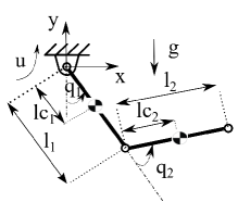
Figure 2: Schematic of Pendubot. Merely the first joint is actuated.

IV-D Pendubot

Here the IDA-PBC method is applied to pendubot system. The robot consists of two revolute joints in which merely the first one is actuated [25]. The schematic of this system is shown in Fig. 2. The dynamic model of the robot may be expressed in the form of (5) with the following matrices [26],

$$M =\begin{bmatrix}c_{1}+c_{2}+2c_{3}\cos(q_{2})&c_{2}+c_{3}\cos(q_{2})\\ c_{2}+c_{3}\cos(q_{2})&c_{2}\end{bmatrix}$$ (23)

$$G =[1,0]^{T},\quad V=-c_{4}g\cos(q_{1})-c_{5}g\cos(q_{1}+q_{2}),$$

where the constants $c_{i}$s are given as follows

$$c_{1} =m_{1}l_{c1}^{2}+m_{2}l_{1}^{2}+I_{1},\quad c_{2}=m_{2}l_{c2}^{2}+I_{2},$$

$$c_{3} =m_{2}l_{1}l_{c2},\quad c_{4}=m_{1}l_{c1}+m_{2}l_{1},\quad c_{5}=m_{2}l_{c2}.$$

In [26], it is shown that the corresponding KE-PDE given in (II) is simplified to the following equation for this system:

$$2c_{3}\sin(q_{2})\big{(}\lambda_{3}^{2}+\lambda_{3}\lambda_{4}\big{)}$$

$$+\lambda_{4}\frac{d}{dq_{2}}\Big{(}\lambda_{3}\big{(}c_{2}+c_{3}\cos(q_{2})\big{)}+\lambda_{4}c_{2}\Big{)}=0$$ (24)

in which

$$M_{d}M^{-1}:=\begin{bmatrix}\lambda_{1}&\lambda_{2}\\ \lambda_{3}&\lambda_{4}\end{bmatrix}.$$

Note that two other PDEs generated form KE-PDE (II) may be solved by suitable definition of the matrix $J_{2}$. The PE-PDE (10) for this system results in:

$$\lambda_{3}\nabla_{q_{1}}V_{d}+\lambda_{4}\nabla_{q_{2}}V_{d}=c_{5}g\sin(q_{1}+q_{2})$$ (25)

Since, PDE (24) has two unknown variables, for simplicity, assume that $\lambda_{4}=k\lambda_{3}$, and reduce it to the following Pfaffian differential equations:

Let us define $k=-1$ to simplify these equations. The non-homogeneous solution is derived from the following equation

$$\frac{d\lambda_{3}}{\lambda_{3}}=\tan(q_{2})dq_{2},$$

which has the solution $\lambda_{3}=-\frac{1}{\cos(q_{2})}$. Note that the homogeneous solution is trivially found to be $\phi(q_{1})$. The corresponding Pfaffian equations to PDE (25) are given as follows

$$\frac{dq_{1}}{-1}=\frac{dq_{2}}{1}=\frac{dV_{d}}{c_{5}g\cos(q_{2})\sin(q_{1}+q_{2})}$$

The homogeneous solution is $V_{d}=\phi(q_{1}+q_{2})$. In order to compute the non-homogeneous solution, we should derive an equation in the form of

$$f_{1}(q_{1},q_{2})dq_{1}+f_{2}(q_{1},q_{2})dq_{2}+dV_{d}=0,$$ (26)

in which,

$$-f_{1}+f_{2}=c_{5}g\cos(q_{2})\sin(q_{1}+q_{2}),$$

and the following constraint resulted from (15) shall be satisfied

$$\frac{\partial f_{2}}{\partial q_{1}}=\frac{\partial f_{1}}{\partial q_{2}}.$$

Combination of the two above equations yields to the following equation

$$\frac{\partial f_{2}}{\partial q_{1}}-\frac{\partial f_{2}}{\partial q_{2}}=-c_{5}g\cos(q_{1}+2q_{2}).$$

The solution to this equation is $f_{2}=c_{5}g\sin(q_{1}+2q_{2})$. Therefore, the Pfaffian equation (26) yields to

$$\hskip 2.84526pt\Big{(}c_{5}g\sin(q_{1}+2q_{2})-c_{5}g\cos(q_{2})\sin(q_{1}+q_{2})\Big{)}dq_{1}$$

$$+c_{5}g\sin(q_{1}+2q_{2})dq_{2}-dV_{d}=0.$$

Now one can apply the proposed procedure in section III to solve this equation. However, to make it short, rewrite it in the following form

$$c_{5}g\sin(q_{2})\cos(q_{1}+q_{2})dq_{1}+\Big{(}c_{5}g\sin(q_{2})\cos(q_{1}+q_{2})$$

$$+c_{5}g\cos(q_{2})\sin(q_{1}+q_{2})\Big{)}dq_{2}-dV_{d}=0,$$

whose solution may be found easily as

$$V_{d}=c_{5}g\sin(q_{1}+q_{2})\sin(q2).$$

Remark 2

In [26], the simplest solution to this problem is reported, in which $\lambda_{3}$ and $\lambda_{4}$ are set to constant values. Here, a nontrivial solution is derived with enlarged domain of attraction. In [26], it is assumed that $q_{2}\in(-\epsilon,\epsilon)$ with $\epsilon=\arccos(\frac{c_{2}}{c_{3}})$. This limitation is also released in the proposed solution, where $q_{2}\in(-\frac{\pi}{2},\frac{\pi}{2})$.

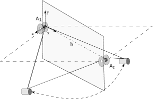
Figure 3: Schematic of underactuated cable driven robots. The end-effector has a swing out of the vertical plane passes from actuators.

IV-E Underactuated spatial cable driven robot

The schematic of this robot is shown in Fig. 3. This system is a planar robot which may have out-of-plane oscillation. Assume that the center of coordinate is located on the first actuator, and the position of actuators are given by:

$$A_{1}=\begin{bmatrix}0&0&0\end{bmatrix}^{T}\qquad\qquad A_{2}=\begin{bmatrix}b&0&0\end{bmatrix}^{T}$$ (27)

Dynamic matrices of the robot may be easily found as

$$M =mI_{3},\qquad\qquad\hskip 5.69054ptV=mgy$$

$$G =\begin{bmatrix}\frac{x}{l_{1}}&\frac{x-b}{l_{2}}\\ \frac{y}{l_{1}}&\frac{y}{l_{2}}\\ \frac{z}{l_{1}}&\frac{z}{l_{2}}\end{bmatrix}\qquad q=\begin{bmatrix}x\\ y\\ z\end{bmatrix}$$ (28)

where $q$ denotes the position of end-effector, $m$ denotes the payload mass, and

$$l_{1}^{2}=x^{2}+y^{2}+z^{2},\qquad l_{2}^{2}=(x-b)^{2}+y^{2}+z^{2}.$$

Furthermore, assume that the cables are massless and infinitely stiff. The equilibrium points of the robot are $q^{*}=[x^{*},y^{*},0]$. Since these are natural equilibrium points of the robot, one may use potential energy shaping for the controller design. However, in this work we try to shape the total energy of the system for a broader representation. For this robot, KE-PDE introduced in (II) yields to:

$$G^{\bot}\{-m^{-1}M_{d}\nabla_{q}(p^{T}M_{d}^{-1}p)+2J_{2}M_{d}^{-1}p\}=0,$$

with

$$G^{\bot}=\begin{bmatrix}0&-bz&by\end{bmatrix}.$$

As explained in [9], the general solution of KE-PDE is obtained from the following equation

$$\displaystyle\sum_{i=1}^{n}\gamma_{i}(q)\frac{dM_{d}^{-1}}{dq_{i}}=-[\mathcal{J}(q)A^{T}(q)+A(q)\mathcal{J}^{T}(q)]$$ (29)

where

$$J_{2} =\begin{bmatrix}0&\tilde{p}^{T}\alpha_{1}&\tilde{p}^{T}\alpha_{2}&\dots&\tilde{p}^{T}\alpha_{n-1}\\ -\tilde{p}^{T}\alpha_{1}&0&\tilde{p}^{T}\alpha_{n}&\dots&\tilde{p}^{T}\alpha_{2n-3}\\ \vdots&\vdots&\vdots&\ddots&\vdots\\ -\tilde{p}^{T}\alpha_{n-1}&-\tilde{p}^{T}\alpha_{2n-3}&\dots&&0\end{bmatrix},$$

$$\tilde{p} =M^{-1}p,\quad\mathcal{J}=[\alpha_{1}\vdots\alpha_{2}\vdots\cdots\vdots\alpha_{n_{0}}]\in\mathbb{R}^{n\times n_{0}},$$

$$A =-[W_{1}(G^{\bot})^{T},\dots,W_{n_{0}}(G^{\bot})^{T}]\in\mathbb{R}^{n_{0}\times n},$$

$$\gamma =G^{\bot}M_{d}M^{-1}.$$

In order to define $W_{i}$s, one may define matrices $F^{kl}$ with $k,l\in\{1,...,n\}$ as follows

$$F^{kl}_{ij}=\begin{cases}1\quad\mbox{if}\quad j>i,i=k\hskip 2.84526pt\mbox{and}\hskip 2.84526ptj=l\\ 0\quad\mbox{otherwise}\end{cases}$$

and set $W^{kl}=F^{kl}-(F^{kl})^{T}$ while $W_{i}$s as

$$W_{1}=W^{12},W_{2}=W^{13},...,W_{n_{0}}=W^{(n-1)n}.$$

By this means one should solve the following PDE:

$$(-zM_{d_{22}}+yM_{d_{23}})\frac{\partial M_{d}}{\partial y}+(-zM_{d_{23}}+yM_{d_{33}})\frac{\partial M_{d}}{\partial z}$$

$$=m\begin{bmatrix}2(-z\alpha_{1_{1}}+y\alpha_{2_{1}})&*&*\\ -z\alpha_{2_{1}}+y(\alpha_{2_{2}}+\alpha_{3_{1}})&2y\alpha_{3_{2}}&*\\ y\alpha_{2_{3}}+z(\alpha_{3_{1}}-\alpha_{1_{3}})&y\alpha_{3_{3}}+z\alpha_{3_{2}}&2z\alpha_{3_{3}}\end{bmatrix},$$ (30)

where the $*$’s in the last matrix denote that it is symmetric. It is clear that $M_{d_{11}},M_{d_{12}},M_{d_{13}}$ may be found arbitrary and the remaining terms shall satisfy the following equations

$$(-zM_{d_{22}}+yM_{d_{23}})\frac{\partial M_{d_{22}}}{\partial y}+(-zM_{d_{23}}+yM_{d_{33}})\frac{\partial M_{d_{22}}}{\partial z}$$

$$=2my\alpha_{3_{2}},$$

$$(-zM_{d_{22}}+yM_{d_{23}})\frac{\partial M_{d_{23}}}{\partial y}+(-zM_{d_{23}}+yM_{d_{33}})\frac{\partial M_{d_{23}}}{\partial z}$$

$$=my\alpha_{3_{3}}+mz\alpha_{3_{2}},$$

$$(-zM_{d_{22}}+yM_{d_{23}})\frac{\partial M_{d_{33}}}{\partial y}+(-zM_{d_{23}}+yM_{d_{33}})\frac{\partial M_{d_{33}}}{\partial z}$$

$$=2mz\alpha_{3_{3}}.$$ (31)

This is a system of PDEs with two arbitrary function. Hence, it is possible to convert it to a single PDE. However, there is no a simple analytical solution for it.

Apply the proposed Theorem to find the solution for this PDE. In order to convert (31) to Pfaffian equations, substitute first and third equation of (31) in the second equation. This yields to:

$$\frac{dy}{P_{1}}=\frac{dz}{P_{2}}=\frac{dM_{d_{23}}}{R}$$ (32)

with

$$P_{1}=-zM_{d_{22}}+yM_{d_{23}}$$

$$P_{2}=-zM_{d_{23}}+yM_{d_{33}}$$

$$+\frac{y}{2z}(-zM_{d_{22}}\frac{\partial M_{d_{33}}}{\partial y}+yM_{d_{33}}\frac{\partial M_{d_{33}}}{\partial z})$$

$$+\frac{z}{2y}(-zM_{d_{22}}\frac{\partial M_{d_{22}}}{\partial y}+yM_{d_{33}}\frac{\partial M_{d_{22}}}{\partial z})$$

where $M_{d_{22}}$ and $M_{d_{33}}$ are arbitrary functions. Equation (32) is equivalent to the following equation

$$\frac{zdy+ydz}{-z^{2}M_{d_{22}}+y^{2}M_{d_{33}}}=\frac{dM_{d_{23}}}{R}$$ (33)

Note that the left hand side is independent of $M_{d_{23}}$, while $R$ is summation of two terms including a linear term and an independent term with respect to $M_{d_{23}}$. Pfaffian equation (33) is easier to solve if $R$ is independent of $M_{d_{23}}$. Notice that the last two terms in $R$ are fractional and hard to be used in the solution. In other words, notice that $M_{d}$ should be positive definite. Hence, one may consider $M_{d_{22}}$ and $M_{d_{33}}$ as

$$M_{d_{22}}=\frac{y^{2}}{2}+k_{1},\qquad\quad M_{d_{33}}=\frac{z^{2}}{2}+k_{2}$$

where $k_{1},k_{2}>0$ to reduce the complexity. Substitute these values in (33):

$$\frac{zdy+ydz}{k_{2}y^{2}-k_{1}z^{2}}=\frac{dM_{d_{23}}}{k_{2}y^{2}-k_{1}z^{2}}$$

The solution to this simplified equation is $M_{d_{23}}=\frac{1}{2}yz$, hence, the structure of $M_{d}$ shall have the form of

$$M_{d}=\begin{bmatrix}*&*&*\\ *&\frac{y^{2}}{2}+k_{1}&\frac{1}{2}yz\\ *&\frac{1}{2}yz&\frac{z^{2}}{2}+k_{2}\end{bmatrix}$$ (34)

where undefined elements may be determined arbitrarily. Notice that these elements do not appear in PE-PDE.

Potential energy PDE (II) for this robot may be derived as:

$$-bmgz =bm^{-1}(-zM_{d_{22}}+yM_{d_{23}})\frac{\partial V_{d}}{\partial y}$$

$$+bm^{-1}(-zM_{d_{23}}+yM_{d_{33}})\frac{\partial V_{d}}{\partial z}.$$

Substitute (34) in this equation to reach to:

$$-m^{2}gz=-k_{1}z\frac{\partial V_{d}}{\partial y}+k_{2}y\frac{\partial V_{d}}{\partial z}$$

This is a simple PDE, that can be solved easily by Lemma 1. The corresponding Pfaffian equations are

$$\frac{dx}{0}=\frac{dy}{-k_{1}z}=\frac{dz}{k_{2}y}=\frac{dV_{d}}{-m^{2}gz}$$

It is clear that $x=c_{1}$ and $k_{2}y^{2}+k_{1}z^{2}=c_{2}$ are the solutions of the first two equalities. Thus, homogeneous solution of PDE is given as

$$V_{d}=\Phi(x,k_{2}y^{2}+k_{1}z^{2}),$$

and from second and forth term, non-homogeneous solution is obtained as

$$V_{d}=\frac{m^{2}g}{k_{1}}(y-y^{*}).$$

Remark 3

In this example, we have used total energy shaping method for the spatial cable driven robot. Note that to the best of authors’ knowledge, none of the reported results on the topic of total energy shaping of an underactuated robot, e.g. [9, 10, 15] can be used to find the solution.

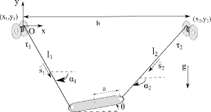
Figure 4: Schematic of planar underactuated cable driven robots. The end-effector has a swing in the plane.

IV-F Underactuated planar cable driven robot

In this Example let us apply IDA-PBC method to a 3-DOF underactuated planar cable driven robot. The schematic of this robot is illustrated in Fig. 4. Dynamic matrices of the robot are in the form of (5) as given in [19]:

$$G^{T}=\begin{bmatrix}\frac{x-a\cos(\theta)}{l_{1}}&\frac{y-a\sin(\theta)}{l_{1}}&\begin{array}[]{c}-a\cos(\theta)\frac{y-a\sin(\theta)}{l_{1}}\\ +a\sin(\theta)\frac{x-a\cos(\theta)}{l_{1}}\end{array}\\ \frac{x-b+a\cos(\theta)}{l_{2}}&\frac{y+a\sin(\theta)}{l_{2}}&\begin{array}[]{c}a\cos(\theta)\frac{y+a\sin(\theta)}{l_{2}}\\ -a\sin(\theta)\frac{x-b+a\cos(\theta)}{l_{2}}\end{array}\end{bmatrix}$$

$$M=\begin{bmatrix}m&0&0\\ 0&m&0\\ 0&0&I\end{bmatrix},V=mgy,\hskip 2.84526ptq=\begin{bmatrix}x\\ y\\ \theta\end{bmatrix}$$

For this robot, the manifold of equilibrium points may be derived as:

$$G^{\perp}\nabla_{q}V=0\quad\implies\quad-2xy\cos(\theta)+by\cos(\theta)$$

$$+ab\sin(\theta)\cos(\theta)+2x^{2}\sin(\theta)-2bx\sin(\theta)=0.$$

As indicated in [19], these points are natural equilibrium points of the system; thus, only potential energy shaping is required.

The PE-PDE (10) for this system is as follows:

$$-ab\sin^{2}(\theta)\Big{)}\frac{\partial V_{d}}{\partial x}+a\Big{(}-2xy\cos(\theta)+by\cos(\theta)$$

$$+ab\sin(\theta)\cos(\theta)+2x^{2}\sin(\theta)-2bx\sin(\theta)\Big{)}\frac{\partial V_{d}}{\partial y}$$

$$+\Big{(}2ax\sin(\theta)-2ay\cos(\theta)+by-ab\sin(\theta)\Big{)}\frac{\partial V_{d}}{\partial\theta}$$ (35)

Finding the solution to this PDE is a prohibitive task. However, it can be solved in a systematic way using the proposed method in section III. Corresponding Pfaffian differential equation is:

$$\frac{dx}{P_{1}}=\frac{dy}{P_{2}}=\frac{d\theta}{P_{3}}=\frac{dV_{d}}{mgP_{2}}$$ (36)

with

$$P_{1}=a\big{(}2\cos(\theta)y^{2}-2\sin(\theta)xy+by\sin(\theta)-ab\sin^{2}(\theta)\big{)}$$

$$P_{2}=a\big{(}-2xy\cos(\theta)+by\cos(\theta)+ab\sin(\theta)\cos(\theta)$$

$$\hskip 14.22636pt+2x^{2}\sin(\theta)-2bx\sin(\theta)\big{)}$$

$$P_{3}=\big{(}2ax\sin(\theta)-2ay\cos(\theta)+by-ab\sin(\theta)\big{)}.$$

To compute the homogeneous solution, let us derive a Pfaffian equation that satisfies condition (15). For this purpose, and considering (35), it is reasonable to derive a Pfaffian equation whose corresponding coefficients of $dx$ and $dy$ are merely function of $\theta$. Hence, let’s start with the following expression to omit $x^{2}$ and $y^{2}$ from denominator

$$\big{(}4a\cos(\theta)\big{)}dx+\big{(}4a\sin(\theta)\big{)}dy+\big{(}-4a\sin(\theta)x$$

$$+4a\cos(\theta)y\big{)}d\theta,$$ (37)

which results in

$$=Eq.(\ref{11})$$

In this equation $x^{2}$ was omitted. To omit $y^{2}$, first add $-2bdx$ to (IV-F) and then add $2ab\sin(\theta)d\theta$ to it:

$$+\frac{-2bdx+2ab\sin(\theta)d\theta}{0}=Eq.(\ref{11})$$

Thus, the nominator shall be zero, and by this means, one can easily verify that condition (15) holds. Although solving the Pfaffian equation

$$\big{(} 4a\cos(\theta)-2b\big{)}dx+\big{(}4a\sin(\theta)\big{)}dy+\big{(}-4a\sin(\theta)x$$

$$+4a\cos(\theta)y+2ab\sin(\theta)\big{)}d\theta=0,$$ (38)

is not hard, let us apply the procedure proposed in section III to find the solution in a systematic manner.

$$U\big{(}(4a\cos(\theta)-2b)x+4a\sin(\theta)y\big{)}=C,\qquad\mu=1$$

$K$ is derived as

$$K=R+4a\sin(\theta)x-4a\cos(\theta)y=2ab\sin(\theta).$$

Finally, by using Lemma 1, the solution is given by

$$V_{d}=\phi\Big{(}U-2ab\cos(\theta)\Big{)} =\Phi\Big{(}\big{(}4a\cos(\theta)-2b\big{)}x$$

$$+4a\sin(\theta)y-2ab\cos(\theta)\Big{)}.$$

With a similar approach, we try to get a separable Pfaffian equation in the following form

$$P(x_{1})dx_{1}+Q(x_{2})dx_{2}+R(x_{3})dx_{3}=0,$$

which is easily integrable and has the following solution

$$\phi\bigg{(}\int P(x_{1})dx_{1}+\int Q(x_{2})dx_{2}+\int R(x_{3})dx_{3}\bigg{)}.$$

After some manipulations, the following equation is obtained

$$\frac{xdx+ydy-\frac{b}{2}dx+\frac{ab}{2}\sin(\theta)d\theta}{0}=Eq.(\ref{11})$$ (39)

The solution of (39) is

$$V_{d}=\phi\big{(}x^{2}+y^{2}-\frac{b}{2}x-\frac{ab}{2}\cos(\theta)\big{)}.$$

Notice that since we are shaping the potential energy in here, the non-homogenious solution is equal to the open loop potential energy, i.e. $V_{d}=mgy$.

Remark 4

The fist impression of PDE (35) is very inconvenient, and finding its solution is a prohibitive task, to the best of author’s knowledge not being reported in the literature and it is not possible to solve it using any software. The power of proposed method to restate and reformulate this problem to some Pfaffian differential equation is the key point to solve this challenging problem.

V Conclusions

In this paper, we derived suitable solution to the PDEs arising in controller design methods such as in IDA-PBC. By using the Sneddon’s method, a first-order PDE is represented by some equivalent Pfaffian differential equations. It was shown that if integrability condition holds for a Pfaffian differential equation with three variables, then the solution could be easily found. In order to illustrate how this method can be applied in practice, it was implemented to a number of different benchmark systems through which the IDA-PBC are designed. Although, the systems being investigated in this paper include magnetic levitation system, pendubot and two underactuated cable driven robots, the application of the proposed method is general and is not limited to these case studies.

References

- [1] R. Ortega, A. Van Der Schaft, B. Maschke, and G. Escobar, “Interconnection and damping assignment passivity-based control of port-controlled hamiltonian systems,” Automatica, vol. 38, no. 4, pp. 585–596, 2002.
- [2] A. Qureshi, S. El Ferik, and F. L. Lewis, “L2 neuro-adaptive tracking control of uncertain port-controlled hamiltonian systems,” IET Control Theory & Applications, vol. 9, no. 12, pp. 1781–1790, 2015.
- [3] R. Ortega and E. Garcia-Canseco, “Interconnection and damping assignment passivity-based control: A survey,” European Journal of control, vol. 10, no. 5, pp. 432–450, 2004.
- [4] A. Donaire, J. G. Romero, R. Ortega, B. Siciliano, and M. Crespo, “Robust ida-pbc for underactuated mechanical systems subject to matched disturbances,” International Journal of Robust and Nonlinear Control, vol. 27, no. 6, pp. 1000–1016, 2017.
- [5] S. Muhammad and A. Dòria-Cerezo, “Passivity-based control applied to the dynamic positioning of ships,” IET control theory & applications, vol. 6, no. 5, pp. 680–688, 2012.
- [6] A. M. Bloch, N. E. Leonard, and J. E. Marsden, “Controlled lagrangians and the stabilization of mechanical systems. i. the first matching theorem,” IEEE Transactions on automatic control, vol. 45, no. 12, pp. 2253–2270, 2000.
- [7] Y. Gupta, K. Chatterjee, and S. Doolla, “Controller design, analysis and testing of a three-phase vsi using ida–pbc approach,” IET Power Electronics, vol. 13, no. 2, pp. 346–355, 2019.
- [8] E. Franco, “Ida-pbc with adaptive friction compensation for underactuated mechanical systems,” International Journal of Control, pp. 1–11, 2019.
- [9] J. A. Acosta, R. Ortega, A. Astolfi, and A. D. Mahindrakar, “Interconnection and damping assignment passivity-based control of mechanical systems with underactuation degree one,” IEEE Transactions on Automatic Control, vol. 50, no. 12, pp. 1936–1955, 2005.
- [10] G. Viola, R. Ortega, R. Banavar, J. Á. Acosta, and A. Astolfi, “Total energy shaping control of mechanical systems: simplifying the matching equations via coordinate changes,” IEEE Transactions on Automatic Control, vol. 52, no. 6, pp. 1093–1099, 2007.
- [11] J. Á. Acosta and A. Astol, “On the pdes arising in ida-pbc,” in Proceedings of the 48h IEEE Conference on Decision and Control (CDC) held jointly with 2009 28th Chinese Control Conference. IEEE, 2009, pp. 2132–2137.
- [12] K. Nunna, M. Sassano, and A. Astolfi, “Constructive interconnection and damping assignment for port-controlled hamiltonian systems,” IEEE Transactions on Automatic Control, vol. 60, no. 9, pp. 2350–2361, 2015.
- [13] A. Donaire, R. Ortega, and J. G. Romero, “Simultaneous interconnection and damping assignment passivity-based control of mechanical systems using dissipative forces,” Systems & Control Letters, vol. 94, pp. 118–126, 2016.
- [14] P. Borja, R. Cisneros, and R. Ortega, “Shaping the energy of port-hamiltonian systems without solving pde’s,” in 2015 54th IEEE Conference on Decision and Control (CDC). IEEE, 2015, pp. 5713–5718.
- [15] A. Donaire, R. Mehra, R. Ortega, S. Satpute, J. G. Romero, F. Kazi, and N. M. Singh, “Shaping the energy of mechanical systems without solving partial differential equations,” in 2015 American Control Conference (ACC). IEEE, 2015, pp. 1351–1356.
- [16] R. Mehra, S. G. Satpute, F. Kazi, and N. M. Singh, “Control of a class of underactuated mechanical systems obviating matching conditions,” Automatica, vol. 86, pp. 98–103, 2017.
- [17] I. N. Sneddon, Elements of partial differential equations. Courier Corporation, 2006.
- [18] L. C. Evans, Partial differential equations. American Mathematical Soc., 2010, vol. 19.
- [19] M. R. J. Harandi, H. Damirchi, H. D. Taghirad et al., “Point-to-point motion control of an underactuated planar cable driven robot,” in 2019 27th Iranian Conference on Electrical Engineering (ICEE). IEEE, 2019, pp. 979–984.
- [20] M. R. J. Harandi and H. Taghirad, “Solution to ida-pbc pdes by pfaffian differential equations,” arXiv preprint arXiv:2006.14983, 2020.
- [21] R. Ortega, A. J. Van Der Schaft, I. Mareels, and B. Maschke, “Putting energy back in control,” IEEE Control Systems Magazine, vol. 21, no. 2, pp. 18–33, 2001.
- [22] K. P. Tee, S. S. Ge, and E. H. Tay, “Barrier lyapunov functions for the control of output-constrained nonlinear systems,” Automatica, vol. 45, no. 4, pp. 918–927, 2009.
- [23] B. Borovic, C. Hong, A. Q. Liu, L. Xie, and F. L. Lewis, “Control of a mems optical switch,” in 2004 43rd IEEE Conference on Decision and Control (CDC)(IEEE Cat. No. 04CH37601), vol. 3. IEEE, 2004, pp. 3039–3044.
- [24] R. Ortega, A. Astolfi, G. Bastin, and H. Rodriguez, “Stabilization of food-chain systems using a port-controlled hamiltonian description,” in Proceedings of the 2000 American Control Conference. ACC (IEEE Cat. No. 00CH36334), vol. 4. IEEE, 2000, pp. 2245–2249.
- [25] Z. Wang and Y. Guo, “Unified control for pendubot at four equilibrium points,” IET control theory & applications, vol. 5, no. 1, pp. 155–163, 2011.
- [26] J. Sandoval, R. Ortega, and R. Kelly, “Interconnection and damping assignment passivity—based control of the pendubot,” IFAC Proceedings Volumes, vol. 41, no. 2, pp. 7700–7704, 2008.