Performance of ALICE AD modules in the CERN PS test beam

Abstract

Two modules of the AD detector have been studied with the test beam at the T10 facility at CERN. The AD detector is made of scintillator pads read out by wave-length shifters (WLS) coupled to clean fibres that carry the produced light to photo-multiplier tubes (PMTs). In ALICE the AD is used to trigger and study the physics of diffractive and ultra-peripheral collisions as well as for a variety of technical tasks like beam-gas background monitoring or as a luminometer.

The position dependence of the modules’ efficiency has been measured and the effect of hits on the WLS or PMTs has been evaluated. The charge deposited by pions and protons has been measured at different momenta of the test beam. The time resolution is determined as a function of the deposited charge. These results are important ingredients to better understand the AD detector, to benchmark the corresponding simulations, and very importantly they served as a baseline for a similar device, the Forward Diffractive Detector (FDD), being currently built and that will be in operation in ALICE during the LHC Runs 3 and 4.

1 Introduction

ALICE (A Large Ion Collider Experiment) [1] is one of the four main detectors at the CERN Large Hadron Collider (LHC). It is designed to study strongly interacting matter at the highest energy densities reached so far in the laboratory, using proton–proton, proton–nucleus and nucleus–nucleus collisions [2]. In addition to its main physics program, ALICE is also an excellent detector to study other aspects of quantum chromodynamics (QCD) such as diffraction [3] and photon-induced interactions [4].

ALICE started operation in 2009 and has been taken data since then during the so-called Run 1 (2009-2013) and Run 2 (2015-2018). Even though during these years the performance of the detector has been excellent [5], a large part of the current ALICE-Detector setup would not be able to cope with the conditions expected at the LHC in Run 3 and 4. In order to exploit the increased luminosity and interaction rate in this period, ALICE is now implementing a significant upgrade of its detectors and systems [6].

Among the detectors being upgraded is the ALICE Diffractive (AD) detector [7], whose new implementation is known as the Forward Diffraction Detector (FDD). Both detectors are composed of two arrays installed at each side of the nominal interaction point in ALICE. Each array is made of 4 sectors, which are made of two layers of identical modules. Each module is made of a plastic scintillator pad, wave-length shifters (WLS), optical fibres and photo-multiplier tubes (PMTs). Both detectors have the exact same geometry, but the materials of the FDD are faster. Here, the main contribution comes from the WLS bar re-emission time that will be reduced from 8.5 ns to 0.9 ns. At the same time, the news PMTs have 19 dynodes (instead 16 as the AD PMTs) which will reduce after-pulses and also have a more extensive dynamic range. Both the AD and the FDD cover the same pseudorapidity ($\eta$) ranges of $-6.9<\eta<-4.9$ and $4.7<\eta<6.3$. Furthermore, the FDD will be also equipped with the possibility of having continuous read-out [8] in addition to the standard trigger mode. The main tasks carried out by the AD and to be taken over by the FDD are to participate at the level zero of the trigger system of ALICE, to provide physics information for the analysis of diffractive and ultra-peripheral collisions and to contribute technical measurements like beam-background monitoring, act as a luminometer, measure the centrality in collisions of heavy nuclei and others.

This article reports the analysis of several test-beam measurements which were carried out with two AD modules to determine their characteristics and performance. The data was collected in 2015 at the T10 PS beam at CERN to study the efficiency, time resolution and charge measurement of these modules. These results are not only needed to understand better the response of the AD detector—used in many ongoing analyses of ALICE data from Run 2—, but also to learn about the potential of the new FDD. The rest of this article is organised as follows: in Sec. 2 the trigger configuration and the placement of the AD detectors in the experimental set-up are described. Sec. 3 reports the results of the analysis of the efficiency, time response and charge measurement obtained with the different components of the detector, and when relevant as a function of the beam energy and and the type of particles—pions and protons— delivered by the beam. Finally in Sec. 4, the conclusions of these studies are summarised.

2 Experimental set-up

Two modules, denoted as ADA  and ADC, were tested. They are shown in Fig. 1. The ADA  and ADC  modules are identical to the modules used in ALICE at positive and negative pseudorapidities, respectively. These modules are made of Bicron BC-404 plastic scintillator, with WLS bars Eljen EJ-208 in two of the sides. The bars are coupled to clear fibres leading the light to Hamamatsu R5946 PMTs. The lengths of the optical fibres were shorter in the test beam, where 47 cm-long fibers were used for both modules instead of 100 cm and 54 cm for ADA-type modules, and 250 cm for ADC-type modules. The different lengths are due to the available space and the placement requirements in the ALICE cavern and LHC tunnel, where the detectors are placed, but which were not present during the studies with the test beam. During the test the PMTs were operated at 1500 and 1650 V for ADA  and ADC, respectively. The read-out was also identical to the one installed in ALICE [9]; in particular, the signal from the AD modules was split into two signals, one to measure the deposited charge and the other, amplified by ten, to determine the arrival time of the particles.

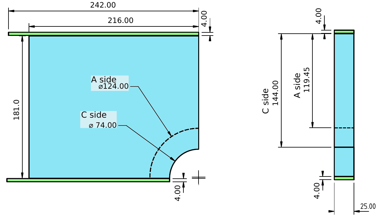
Figure 1: Drawing of the plastic scintillator pads (blue) and WLS bars (green) of the ADA  and ADC  detectors. The difference between the modules is the radius of the cut in the corner to accommodate the beam-pipe: ADA (ADC) has a 124 (74) mm radius cut. Therefore the bars attached to the side of the cut, have different lengths: 182 and 207 mm for the ADA  and ADC  modules, respectively.

The T10 beam at the Proton Synchrotron (PS) machine [10] was used as a source. The beam consisted mainly of pions ($\pi^{+}$) and protons ($p^{+}$). The following beam momenta were chosen: 1.0, 1.5, 2.0 and 6 GeV/$c$. The relative momentum resolution was 1.3%.

The set-up for the data taking in the test beam is shown in Fig. 2. In addition to the AD modules, one can also see two other scintillator modules labelled black-start and black-end, as well as two Cherenkov radiators denoted as T0-start and T0-end [11]. These devices were used to provide triggers and reference timing for the measurements presented below. The specific configurations for these tasks depended on the measurement being carried out and are described in the corresponding sections.

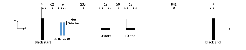
Figure 2: Test beam set-up in the T10 beam line. The beam direction goes from left to right. All distances are given in centimetres. The drawing is not to scale.

The final device involved in the measurements was a silicon pixel sensor positioned at the edge of the scintillator pad, as shown in Fig. 3. This detector has an ALPIDE chip as those used for the upgrade of the Inner Tracking System [12] and for the new Muon Forward Tracker [13] of ALICE. The chip is based on the CMOS MAPS technology; it has an array of $512\times 1024$ pixels with a size of $26.88\times 29.24\,\mu\textrm{m}^{2}$ and a sensitive area of $1.376\times 3.0\,\textrm{cm}^{2}$.

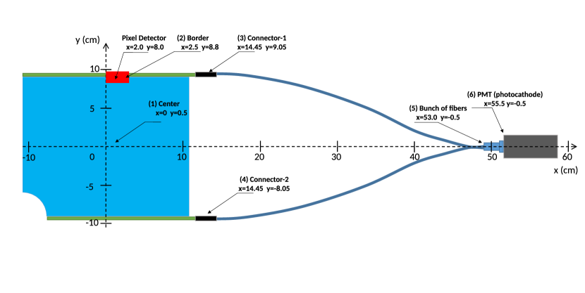
Figure 3: Location of the scintillator, the WLS bars, the fibres, the PMT, and the pixel detector, as well as the definition of the coordinate system whose origin lies at the centre of the plastic scintillator.

3 Results

3.1 Efficiency

The efficiency is defined as the fraction of events selected according to Eq. (1):

$$P(\textrm{AD}|\textrm{T0-start}\wedge\textrm{T0-end})=\frac{N_{\textrm{AD}}}{N_{\textrm{T0}}}=\frac{N(\textrm{AD}\wedge\textrm{T0-start}\wedge\textrm{T0-end})}{N(\textrm{T0-start}\wedge\textrm{T0-end})}$$ (1)

where $N_{\textrm{AD}}$ is the number of events that fulfilled the 3-fold coincidence condition, defined by the logic AND between T0-start, T0-end and the AD module, while $N_{\textrm{T0}}$ is the total number of events given by the 2-fold coincidence between the T0-start and T0-end. All the triggers are given by the time signal, in particular the ADA  and ADC  modules are triggered when the time signal is below a $-40$ mV threshold and inside a 15 ns time window [9]. (This time-window in the electronics is designed to tag beam–beam interaction in the ALICE experiment.) The statistical uncertainty is computed as

$$\delta=\sqrt{P(1-P)/N_{\textrm{T0}}}\quad\textrm{where}\quad P=N_{\textrm{AD}}/N_{\textrm{T0}}.$$ (2)

The first measurement to be presented is the efficiency to detect the incoming particles as a function of the impact position, quantified by the centre of the beam spot. The detector was placed over a movable table which could be displaced perpendicular to the beam line such that the beam spot could be made to interact at specific positions in the module. For these studies the beam momentum was set at 1 GeV/$c$.

The results are shown in Fig. 4. Both detectors are around to $~{}99.8$% efficient for most of the positions sampled. For the scan on the $Y$ direction some positions were skipped due to time limitations to use the beam line and because at that point it was already clear that the efficiency is flat also along this axis. The drop of the efficiency at the border and the existence of an apparent non-zero efficiency outside the nominal acceptance of the module is explained by the size of the beam spot.

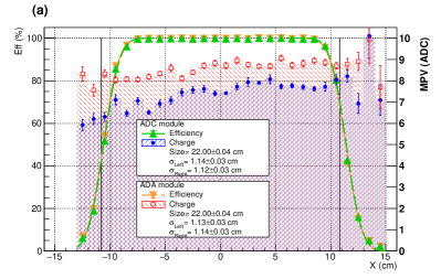
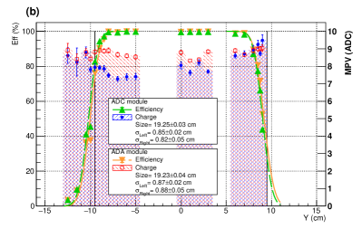
Figure 4: The efficiency, as defined in Eq. (1), of the AD modules as a function of the position of the beam spot according to the reference system depicted in Fig. 3 is shown with the green and orange symbols and the scale in the left vertical axis. The MPV as defined in Sec. 3.2 is shown with the red and blue markers and the right vertical axis. See text for details.

To quantify the size of the beam and the corresponding shape of the efficiency curves a Gaussian Cumulative Function distribution (CDF) is used [14]

$$F(X|\mu,\sigma)=\frac{1}{\sigma\sqrt{2\pi}}\displaystyle\int_{-\infty}^{X}e^{\frac{-(t-\mu)^{2}}{2\sigma^{2}}}\,dt$$ (3)

This CDF is adjusted to the edges of the efficiency curves. The physical length in the vertical and horizontal axes of both modules are calculated using the differences between the distances of the mean values of the CDF for each case, obtaining a length of $X=22\pm 0.1$ cm and $Y=19\pm 0.1$ cm for each axis, which are consistent with the physical length of the modules convoluted with the beam size. The value of the $\sigma$ parameter for the left and right CDF corresponding to each axis are consistent and are averaged to estimate the beam size of each axis to obtain $\sigma_{Y}=1.13\pm 0.06$ cm and $\sigma_{X}=0.86\pm 0.08$ cm.

In order to determine the efficiency at the border of the detector, and to verify that impacts in the WLS bar can be ignored, the silicon pixel sensor is used. The detector is placed so that it covers part of the plastic scintillator and of the WLS bar as shown in Fig. 3. Data taking is triggered by a coincidence in the black-start and black-end scintillators. In this case, the efficiency is defined as:

$$P(\textrm{AD}|\textrm{black-start}\wedge\textrm{black-end}\wedge\textrm{Pixel})=\frac{N(\textrm{AD}\wedge\textrm{black-start}\wedge\textrm{black-end}\wedge\textrm{Pixel})}{N(\textrm{black-start}\wedge\textrm{black-end}\wedge\textrm{Pixel})}$$ (4)

The results are shown in Fig. 5. Adjusting a the CDF of Eq. (3) the parameters obtained are: $\mu_{A}=0.38$ cm, $\sigma_{A}=0.036$ cm, $\mu_{C}=0.59$ cm and $\sigma_{C}=0.035$ cm, where the A and C index denote the parameters of the A and C modules. Additionally, a misalignment of approximately 0.21 cm between the two detectors can be seen in the figure. It is worth to mention that for ADC  the background shown below 0.55 cm and the small inefficiency for the places above 0.65 cm are attributed to noisy pixels; the same is valid for ADA, but the background is below 0.34 cm and the inefficiencies are above 0.45 cm.

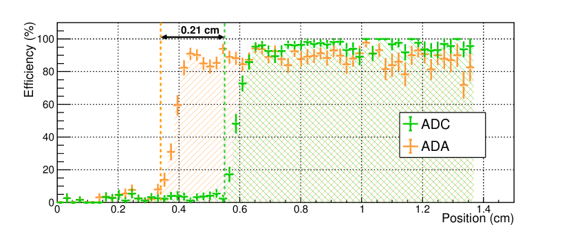
Figure 5: Detection efficiencies along the vertical axis (Y-axis) of ADC  (green) and ADA  (orange) near the edge determined with the silicon pixel sensor.

Finally, the efficiency when the beam hits other elements, like the optical connectors, the fibre bundles or the PMT has also been studied. The efficiency to detect a signal for particles hitting the optical connectors (see Fig. 3) is the same in ADA  and ADC  and amounts to 5% for the connector at a $Y$ position of $-8.05$ cm, while it raises to 10% for the connector at $Y=9.05$ cm. The efficiency when the fibre bundle at $X=53$ cm is scanned from $Y=-3$ cm to $Y=3$ cm has a maximum of 15% (ADA) and 10% (ADC) at $Y=-0.5$ cm and decays rapidly towards zero within some 1.5 cm. The efficiency when the beam hits at $X=55.5$ cm, corresponding to the face of the PMT, is 40% and decays rapidly with increasing $X$, reaching zero at $X=60$ cm.

3.2 Charge measurement

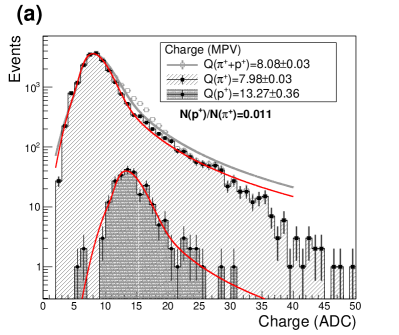
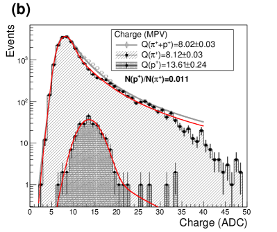
Figure 6: Charge distributions of the (a) ADC  and (b) ADA  modules for a 1 GeV/$c$ beam momentum for all particles, and for pions and protons separately. The lines represent a fit to the model mentioned in the text.

An example of the charge distribution in the ADA  and ADC  modules is shown in Fig. 6 along with a model based on the sum of a Landau with a Gaussian distribution, where the most probable value (MPV) of the Landau and mean of the Gaussian distributions are constrained to be the same. The Gaussian distribution serves to describe detectors effects which smear the charge distribution. The data represented by the light-gray square markers in Fig. 6 corresponds to events triggered by the 3-fold coincidence given by $N_{\textrm{AD}}$ in Eq. (1) and were recorded with a beam momentum of 1 GeV/$c$. The most probable value (MPV) is a bit larger than 8 ADC channels.

This type of distribution is used to extract the MPV as a function of the impact point of the beam spot in the detector. This is shown in Fig. 4 with the blue and red markers and the scale in the right-side axes. One observes a slightly different value of the MVP in the ADA  and the ADC  detectors. This is a geometric effect of the light propagation in the scintillator, because the ADA  detector misses a larger semicircle than the ADC  module as seen in Fig. 1. The slight dependence on the coordinates of the impact point of the beam spot is also due to the same geometric effect.

The dependences of the MPV on the particle type and on the momentum of the beam have also been studied. The first is illustrated in Fig. 6, while the latter is shown in Table 1. The figure shows the case of a beam momentum of 1 GeV/$c$. There is a clear separation between the MPV of both particles, where as expected the protons produce more charge than the pions. (The particle identification using the time-of-flight technique is discussed below.) The table presents the MPV for both particles as a function of the beam momentum. In the case of pions the MPV grows slightly with energy, while for protons the opposite behaviour is observed. This behavior is roughly expected, since in this region of the Bethe Bloch curve the protons go through the MIP and the pions are already in the relativistic rise.

Table 1: MPV of the charge measured for pions, protons and the sum of both. For a momentum of 6 GeV/$c$ it is not possible to distinguish the particles using the time-of-flight technique described in the text.

Momentum	Charge (ADC counts)
(GeV/$c$)	ADC			ADA
	$\pi^{+}+p^{+}$	$\pi^{+}$	$\textrm{p}^{+}$	$\pi^{+}+p^{+}$	$\pi^{+}$	$\textrm{p}^{+}$
1.0	8.08$\pm$0.03	7.98$\pm$0.03	13.27$\pm$0.036	8.02$\pm$0.03	8.12$\pm$0.03	13.61$\pm$0.24
1.5	8.3$\pm$0.04	8.18$\pm$0.04	9.72$\pm$0.16	8.56$\pm$0.05	8.45$\pm$0.05	9.94$\pm$0.13
2.0	8.21$\pm$0.02	8.12$\pm$0.02	8.80$\pm$0.06	8.41$\pm$0.02	8.35$\pm$0.02	8.89$\pm$0.06
6.0	7.23$\pm$0.09	-	-	7.14$\pm$0.08	-	-

3.3 Time resolution

To measure the time resolution one needs two ingredients. First a reference time, and second a correction for the the measured time as a function of the deposited charge, the so-called time slewing. In the set-up shown in Fig. 2 the Cherenkov detectors have the best time resolution, below 50 ps [11], so it is natural to use the T0-end to provide the reference time. Comparing the times of T0-end and the black-start detector it is possible to have a clean separation of the pion and proton components of the beam as demonstrated below, so that the analysis can be done for each particle type separately.

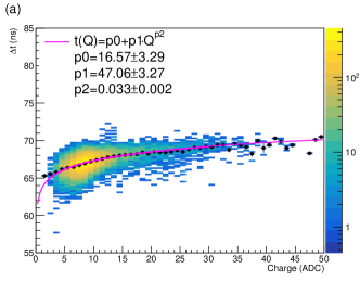
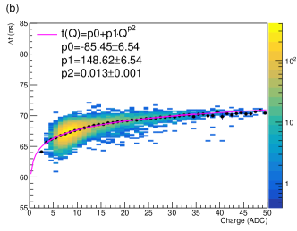
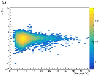
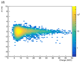
Figure 7: Time slewing correction calculated using the pions distributions of ADC  (a) and ADA  (b). The corrected distributions of ADC  and ADA  can be seen in (c) and (d) histograms respectively.

The time measurements are affected by the slewing effect which can be corrected for as follows [15]. The case of pions is used to illustrate the correction, because the effect is the clearest of both cases. The (a) and (b) histograms of Fig. 7 show the correlation between the time and the charge measured with the ADA  and ADC  modules. A clear dependence is seen that can be parameterised as $t(Q)=p0+p1\cdot Q^{p2}$ where $p0$, $p1$, and $p2$ are parameters. The corrected time is calculated subtracting the time $t(Q)$ to the measured time: $t(\textrm{corr.})=t(\textrm{measured})-t(Q)$, where $t(\textrm{corr.})$ is the time corrected and $t(\textrm{measured})$ is the time measured in each individual event. The corrected distributions are shown in the (c) and (d) histograms of the same figure.

The effect that this correction has on the time resolution can be seen in Fig. 8 for the case of a beam momentum of 1 GeV/$c$. The mean time difference for both particle species is obtained from the difference in mean values of the Gaussian distributions fitted to each contribution.

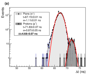
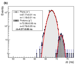
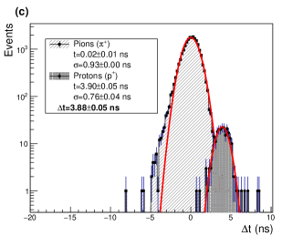
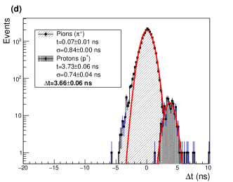
Figure 8: Time-of-flight difference between AD and the T0-end detector ($\Delta t=t_{\textrm{AD}}-t_{\textrm{T0-end}}$) for a 1 GeV/$c$ beam momentum, and Gaussian fits to the pions and protons contributions. The top panels show the uncorrected ADC (a) and ADA (b) time difference. Similarly, the bottom row shows the ADC (c) and ADA (d) time differences after applying the time slewing correction.

Table 2: Time resolutions of ADC and ADA at different momenta of pions and protons after the time slewing correction.

Momentum	$\sigma$ (ns)
(GeV/c)	ADC		ADA
	$\pi^{+}$	$\textrm{p}^{+}$	$\pi^{+}$	$\textrm{p}^{+}$
1.0	0.93$\pm$0.01	0.76$\pm$0.04	0.84$\pm$0.01	0.74$\pm$0.04
1.5	1.26$\pm$0.02	1.18$\pm$0.07	1.17$\pm$0.02	1.19$\pm$0.06
2.0	1.32$\pm$0.01	1.40$\pm$0.04	1.22$\pm$0.01	1.33$\pm$0.02
6.0	1.12$\pm$0.02		1.18$\pm$0.02

A summary of the time resolutions obtained for the different beam momenta is shown in Table 2. The resolution is similar for both detectors. It increases with momentum and it is larger for pions than for protons. For the lower beam momentum, the resolution is below 1 ns and remains well below 1.5 ns even at the largest beam momentum.

Finally, the dependence of the time resolution on the deposited charge for pions at 1 GeV/$c$ is shown in Fig. 9. This dependency is obtained dividing the charge spectrum of the $\pi^{+}$ at 1 GeV/$c$ in seven slices, each of them corresponds to an interval of 5 ADC counts. The resolutions correspond to the standard deviations ($\sigma$) of a Gaussian function fitted to the time distribution corresponding to each slice.

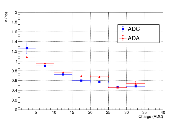
Figure 9: Time resolution as a function of the measured charge for the AD modules in the test beam.

3.4 Simple model for the time of flight and the energy deposition

Here, a simple model is introduced to describe the interaction of the particles in the beam with the detectors in the experimental set-up. First, the time of flight of a particle is computed and then compared to the measurements to validate the model. Once this is done, the model can be used to obtain the energy corresponding to the MPV of the charge distribution.

The first step is to obtain a proper accounting of the time traveled by a given particle while traversing the experimental set-up shown in Fig. 2. The total distance is separated in stages: from black-start to ADC  (65.5 cm), then to ADA  (3 cm), to T0-start (240.5 cm), to T0-end (62 cm), and finally up to black-end (another 854 cm). The distances are taken from the centre of the AD and black scintillators pads and the centre of the quartz radiator of the T0 detectors, adding 1.5 and 2 cm to the distance with respect to the AD and black scintillators respectively; for T0 detectors, we use the distance at 1 cm from the edge facing the beam.

At each stage the change of momentum due to the energy loss when traversing the detector materials is obtained from a Landau distribution [16] where the most probable energy loss is:

$$\Delta_{p}=\xi\left(\ln\frac{2mc^{2}\beta^{2}\gamma^{2}}{I}+\ln\frac{\xi}{I}+j-\beta^{2}-\delta(\beta\gamma)\right)\,\,\,\,\textrm{and}\,\,\,\,\xi=\frac{K}{2}\frac{Z}{A}z^{2}(x/\beta^{2}).$$ (5)

Here the detector thickness is $x$ in g$\cdot$cm^-2, $j=0.2$ and $\delta(\beta\gamma)$ is neglected at low energy; $K=4\pi N_{A}r_{e}^{2}m_{e}c^{2}=0.307075$ MeV $\textrm{mol}^{-1}\,\textrm{cm}^{2}$, $Z$ and $A$ are the atomic and mass number of the material being crossed, $z$ is the charge number of the incident particle, $r_{e}$ the classical electron radius, $m_{e}c^{2}$ the electron mass, $N_{A}$ Avogadro’s number, $I$ the mean excitation energy (eV) and $\delta(\beta\gamma)$ the density effect correction to the ionization energy loss.

The new energy and momentum of the particle is recalculated after each stage using the material budget and $E^{2}=p^{2}c^{2}+M^{2}c^{4}$. The material budget comprises the following: for the AD modules 2.5 cm of Bicron 404 [17] each, while the other scintillators are 4 cm thick. The T0 Cherenkov radiators have a more complex composition being made of a 2 cm thick quartz radiator [11] and a PMT. The PMT is modelled by 1 mm of glass (of the vacuum tube), 1 mm of aluminium for the cover at the front and another 1 mm at the back; in addition the 16 dynodes are represented by a 0.1 mm thick layer of iron.

Finally, the time after each stage is computed as

$$t_{j}=\frac{L}{\beta_{j}c}=\frac{L}{p_{j}c}\sqrt{p_{j}^{2}+m_{j}^{2}c^{2}},$$ (6)

where $j$ indicates the particle (i.e. pion or proton) and $L$ the distance traveled. The time-of-flight difference $\Delta t$ is calculated subtracting the time of flight of the two different particle species traveling the same distance,

$$\Delta t=t_{1}-t_{2}=\frac{L}{c}\left[\left(1+\frac{m_{1}^{2}c^{2}}{p^{2}_{1}}\right)^{1/2}-\left({1+\frac{m_{2}^{2}c^{2}}{p^{2}_{2}}}\right)^{1/2}\right].$$ (7)

Using this model it is possible to compute the expected time differences for the arrival times of a pion and a proton at a given detector. The comparison of the model with the measurement is reported in Table 3 for the case of a 1 GeV/$c$ beam momentum. The agreement is satisfactory for such a simple model of the propagation of the particle beam through the experimental set-up.

Table 3: Theoretical and measured time-of-flight differences between pions and protons for the given distances with respect to the T0-end detector for a 1 GeV/$c$ beam momentum after the time-slewing correction.

Detector	Distance (cm)	$\Delta t$ (ns)
		Theoretical	Measurement
ADC	305.5	3.908	3.9$\pm$0.05
ADA	302.5	3.871	3.66$\pm$0.06
T0.start	62.0	0.907	-
Black.start	371.0	4.715	4.66$\pm$0.03
Black.end	845.0	12.834	14.5$\pm$0.07

Once the model has been validated as producing reasonable results for the time-of-flight difference between pions and protons it can be used to estimate a conversion factor between the ADC charge and the deposited energy. The conversion factor is obtained by dividing the estimated energy deposited in the detector over the charge collected for the detector in each measurement (Table 1). This was done for pion and proton beams with momenta of 1, 1.5 and 2 MeV/$c$. The result is shown in Table 4. The conversion factor is consistent across all cases so it is justified to take the average, which yields

$$\varepsilon=0.832\pm 0.012\,\,\textrm{MeV/ADC},$$ (8)

where the uncertainty is obtained from the standard deviation of the different factors.

Table 4: Theoretical estimation of the energy deposition and energy per ADC count of pions and protons in the ADA and ADC modules, and the corresponding conversion factor of the energy deposition estimation with respect to the charge measured.

Momentum	Theoretical estimation (MeV)				Conversion factor (MeV/ADC)
(MeV/$c$)	ADC		ADA		ADC		ADA
	$\pi^{+}$	$p^{+}$	$\pi^{+}$	$p^{+}$	$\pi^{+}$	$p^{+}$	$\pi^{+}$	$p^{+}$
1000	6.69	10.89	6.68	10.95	0.838$\pm$0.003	0.820$\pm$0.002	0.823$\pm$0.003	0.805$\pm$0.014
1500	6.85	8.14	6.85	8.16	0.838$\pm$0.004	0.837$\pm$0.014	0.8107$\pm$0.005	0.821$\pm$0.0107
2000	7.00	7.25	6.99	7.26	0.862$\pm$0.002	0.824$\pm$0.006	0.838$\pm$0.002	0.816$\pm$0.006
6000	7.63	6.65	7.63	6.65	-	-	-	-

4 Summary and outlook

One ADA  and one ADC  modules have been studied with test beams. The set-up allows for the measurement of the modules’ efficiencies as a function of the beam impact position, and the measurement of the charge deposition as well as the time resolution of the modules. In particular, these two last properties have been studied as a function of the particle species, pion or proton, and the momentum of the test beam. A simple model of the energy deposition on the material of the set-up traversed by the beam particles allows for the conversion of the ADC charge into an energy.

The results show that the modules have a high and uniform efficiency as a function of the impact point and that the hits in other parts of the detector, like the WLS or the PMT, have a lower efficiency which decays steeply outside of a very small range of positions. The set-up allows to separate the pion and proton components of the beam. The charge deposition in both cases has been measured and shown to behave as expected. The time resolution has been measured and shown to be below 1.5 ns for particles depositing little charge in the modules and below 1 ns for particles depositing more charge.

These results allow for a better understanding of the detector and provide key information to benchmark and improve the simulation of the AD detector used during the LHC Run 2 in ALICE. This knowledge can be applied in a straightforward manner to the the FDD being constructed now and that will be in operation in ALICE during the LHC Runs 3 and 4.

References

- [1] K. Aamodt, et al., The ALICE experiment at the CERN LHC, JINST 3 (2008) S08002. doi:10.1088/1748-0221/3/08/S08002.
- [2] P. Cortese, et al., ALICE: Physics performance report, volume I, J. Phys. G30 (2004) 1517–1763. doi:10.1088/0954-3899/30/11/001.
- [3] B. Abelev, et al., Measurement of inelastic, single- and double-diffraction cross sections in proton–proton collisions at the LHC with ALICE, Eur. Phys. J. C73 (6) (2013) 2456. arXiv:1208.4968, doi:10.1140/epjc/s10052-013-2456-0.
- [4] J. G. Contreras, J. D. Tapia Takaki, Ultra-peripheral heavy-ion collisions at the LHC, Int. J. Mod. Phys. A30 (2015) 1542012. doi:10.1142/S0217751X15420129.
- [5] B. B. Abelev, et al., Performance of the ALICE Experiment at the CERN LHC, Int. J. Mod. Phys. A29 (2014) 1430044. arXiv:1402.4476, doi:10.1142/S0217751X14300440.
- [6] B. Abelev, et al., Upgrade of the ALICE Experiment: Letter Of Intent, J. Phys. G41 (2014) 087001. doi:10.1088/0954-3899/41/8/087001.
- [7] A. Villatoro Tello, AD, the ALICE diffractive detector, AIP Conf. Proc. 1819 (1) (2017) 040020. doi:10.1063/1.4977150.
-
[8]
P. Buncic, M. Krzewicki, P. Vande Vyvre,
Technical Design Report for the
Upgrade of the Online-Offline Computing System, Tech. Rep.
CERN-LHCC-2015-006. ALICE-TDR-019 (Apr 2015).
URL https://cds.cern.ch/record/2011297 - [9] Y. Zoccarato, et al., Front end electronics and first results of the ALICE V0 detector, Nucl. Instrum. Meth. A626-627 (2011) 90–96. doi:10.1016/j.nima.2010.10.025.
-
[10]
D. J. Simon, L. Durieu, K. Bätzner, D. Dumollard, F. Cataneo, M. Ferro-Luzzi,
Secondary beams for tests in the PS
East experimental area, Tech. Rep. PS-PA-EP-Note-88-26, CERN, Geneva (Aug
1988).
URL http://cds.cern.ch/record/1665434 - [11] M. Bondila, et al., ALICE T0 detector, IEEE Trans. Nucl. Sci. 52 (2005) 1705–1711. doi:10.1109/TNS.2005.856900.
- [12] B. Abelev, et al., Technical Design Report for the Upgrade of the ALICE Inner Tracking System, J. Phys. G41 (2014) 087002. doi:10.1088/0954-3899/41/8/087002.
-
[13]
Technical Design Report for the Muon
Forward Tracker, Tech. Rep. CERN-LHCC-2015-001. ALICE-TDR-018 (Jan 2015).
URL https://cds.cern.ch/record/1981898 - [14] N. L. Johnson, S. Kotz, N. Balakrishnan, Continuous univariate distributions / Vol.2, 2nd Edition, New York : Wiley, 1995, previous title: Distributions in Statistics: Continuous Univariate Distributions, v.2.
- [15] E. Abbas, et al., Performance of the ALICE VZERO system, JINST 8 (2013) P10016. arXiv:1306.3130, doi:10.1088/1748-0221/8/10/P10016.
- [16] L. Landau, On the energy loss of fast particles by ionization, J. Phys.(USSR) 8 (1944) 201–205.
- [17] S.-G. Ceramics, I. Plastics, Organic scintillation materials and assemblies, http://www.crystals.saint-gobain.com.