Water Dynamics Around Proteins: T- and R-States of Hemoglobin and Melittin

Abstract

The water dynamics, as characterized by the local hydrophobicity (LH), is investigated for tetrameric hemoglobin and dimeric melittin. For the T₀ to R₀ transition in Hb it is found that LH provides additional molecular-level insight into the Perutz mechanism, i.e., the breaking and formation of salt bridges at the $\alpha_{1}/\beta_{2}$ and $\alpha_{2}/\beta_{1}$ interface is accompanied by changes in LH. For Hb in cubic water boxes with 90 Å and 120 Å edge length it is observed that following a decrease in LH as a consequence of reduced water density or change of water orientation at the protein/water interface the $\alpha/\beta$ interfaces are destabilized; this is a hallmark of the Perutz stereochemical model for the T to R transition in Hb. The present work thus provides a dynamical view of the classical structural model relevant to the molecular foundations of Hb function. For dimeric melittin, earlier results by Cheng and Rossky [Nature, 1998, 392, 696–699] are confirmed and interpreted on the basis of LH from simulations in which the protein structure is frozen. For the flexible melittin dimer the changes in the local hydration can be as much as 30 % than for the rigid dimer, reflecting the fact that protein and water dynamics are coupled.

SABNP, Univ. Evry, INSERM U1204, Université Paris-Saclay, 91025 Evry, France

1 Introduction

Hemoglobin is one of the most widely studied proteins due to its essential role in transporting oxygen from the lungs to the tissues. The two most important structural states of this protein are the deoxy structure (T₀), which is stable when no ligand is bound to the heme-iron, and the oxy structure (R₄), which is stable when each of the four heme groups have a ligand, such as oxygen, bound to them. The state with the quaternary structure of R₄, but with no heme-bound ligands is the R₀ state. Despite strong experimental evidence that T₀ is significantly more stable than R₀, with an equilibrium constant of $K_{\frac{T_{0}}{R_{0}}}=6.7\times 10^{5}$, ¹ molecular dynamics (MD) simulations appear to indicate that the R₀ state is more stable. Specifically, simulations have found that when hemoglobin is initialized in the T₀ state it undergoes a spontaneous transition into the R₀ state on sub-$\mu$s time scales.^{2, 3} Understanding the origins of this discrepancy between the measured and simulated relative stabilities of the R₀ and T₀ states is essential to establishing the reliability of simulation-based studies of Hemoglobin and other large biomolecules.

In a recent simulation study, it was found that the T₀ $\rightarrow$ R₀ transition rate depends sensitively on the size of the simulation cell.⁴ Specifically, simulations of hemoglobin initialized in the T₀ state and placed in a periodically replicated cubic solvent box with side length of 75 Å, 90 Å, and 120 Å, underwent transition towards the R-state structure after 130 ns, 480 ns, and 630 ns, respectively. Furthermore, in a simulation box with side-length of 150 Å, hemoglobin remained in the T₀ state for the entirety of a 1.2$\mu$s simulation. The extrapolated trend in these findings implies that T₀ is the thermodynamically stable state in this largest simulation cell for which the diffusional dynamics of the environment are correctly captured. The results also suggested that such a large box is required for the hydrophobic effect, which stabilizes the T₀ tetramer, to be manifested. While the statistical significance of this conclusion has been a topic of recent discussion in the literature,^{5, 6} the dynamic stability of the T₀ state exhibits a clear systematic dependence on the size of the solvent box. Further analysis is required to provide conclusive evidence of the role of the hydrophobic effect and to reveal the mechanistic origin of the dependence of the thermodynamic stability of the T₀ state on the simulation box size. In this study we specifically address the role of system size variations in solvent dynamics.

The present work addresses the system size question by analyzing the molecular structure of the hydration layers surrounding tetrameric hemoglobin (Hb) and dimeric melittin. The particular focus is on whether there are characteristic changes in local hydration that accompany global transitions involving reorientation of the subunits - i.e. the decay of the T-state for Hb and the reconfiguration of the helices in melittin - and whether and how these changes are effected by the size of the solvent box. Extending the study to the melittin dimer, which is much smaller than Hb, provides information about the generality of this analysis. In addition, melittin was also studied previously as an example for hydrophobic hydration.⁷ Melittin is a small, 26-amino acid protein found in honeybee venom that crystallizes as a tetramer, consisting of two dimers, related by a two-fold symmetry axis.^{8, 9} Previous work has characterized the behaviour of the hydrophobic binding surface of melittin and the solvent exposed surface residues.⁷ While these surface residues are characterized by a well-defined orientation of the water molecules, water molecules in the hydrophobic regions are more dynamical, exploring different water configurations. Here, similar simulations with a frozen melittin dimer in different box sizes are carried out and analyzed. In addition, the protein is also allowed to move freely which provides information about the solvent-solute coupling which has not been considered before.⁷

The analysis is based on a recently developed method of characterizing the hydrophobicity of a surface based on a statistical analysis of the configurational geometries of interfacial water molecules.¹⁰ This method, described in more detail in the “Analysis of Aqueous Interfacial Structure” section, generates an order parameter, $\delta\lambda_{\mathrm{phob}}$, which quantifies the statistical similarity of sampled water configurations to those that occur at equilibrium near an ideal hydrophobic surface. When applied to water configurations sampled from a particular nanoscale region of a protein surface, $\delta\lambda_{\mathrm{phob}}$ can be interpreted as a local measure of hydrophobicity and thus be extended to map the spatial and temporal variations of a protein’s solvation shell.

In the following section the simulations and computational methods are described. Then, in the Results section, analyses and interpretations of protein hydration structure are presented. Results for hemoglobin are described first, including analysis of previous simulations in different simulation box sizes. Results for melittin are described second. Finally, conclusions are drawn.

2 Computational Methods

2.1 Molecular Dynamics Simulations

Simulations of Hemoglobin (Hb): The Hb-simulations (for the sequence see Figure S1) were described previously,⁴ and only the necessary points without technical details are reported here. The molecular dynamics trajectories were run in cubic water boxes with box lengths 90 Å, 120 Å, and 150 Å which are analyzed in the following. Each simulation was run for 1 $\mu$s or longer and for selected box sizes, additional repeat simulations were carried out.⁶ The trajectories analyzed in the present work are those from Ref.⁴ and the reader is referred to that manuscript for additional details on the production runs.

Simulations of Melittin: MD simulations of the melittin dimer were carried out using CHARMM¹¹ c45a1 and the CHARMM36 force field.¹² The TIP3P water model was used, the same as that used for Hb. The dimer structure (PDB:2MLT)¹³ was used as the starting structure. It was solvated in a cubic water box of length 51.051 Å (4066 water molecules) In addition, simulations with a box length of 60 Å were performed to assess whether, in analogy to Hb, there were effects of increased solvent box sizes on the stability, dynamics and water structuring of melittin dimer. A 16 Å cut-off was applied with a Particle Mesh Ewald scheme¹⁴ and a 1 fs time step was used in the MD simulations. Although more physically realistic fixed point charge water models exist (e.g. TIP4P), the use of TIP3P here is mandatory for consistency because the CHARMM force field was parametrized with it. It is certainly of interest to include water polarization in corresponding simulations,¹⁵ but such a study is beyond the scope of the present work.

The following protocol was used. Two steps of minimization were performed: 50 steps with the Steepest Descent algorithm, followed by 50 steps with the Newton-Raphson algorithm. The system was then heated and equilibrated using the velocity Verlet algorithm¹⁶ for 25 ps with a Nose Hoover¹⁷ thermostat at 300 K. This was followed by a 100 ns $NVT$ production simulation, for which coordinates were recorded every 1 ps. In a first set of simulations, the protein dimer was fixed and only the solvent water was allowed to move. This allows direct comparison with the work of Cheng and Rossky.⁷ In a separate set of 100 ns simulations the protein was allowed to move and only bonds involving hydrogen atoms molecules were constrained using SHAKE.¹⁸

2.2 Analysis of Aqueous Interfacial Structure

The hydration structure of the simulated proteins was characterized following a recently developed computational method.¹⁰ This method is based on the concept that deformations in water’s collective interfacial molecular structure encode information about the details of surface-water interactions.¹⁹ These deformations are quantified in terms of the probability distribution of molecular configurations, as specified by the three-dimensional vector, $\vec{\kappa}=(a,\cos{\theta_{\rm OH_{1}}},\cos{\theta_{\rm OH_{2}}})$, where $a$ is the distance of the oxygen atom position to the nearest point on the instantaneous water interface, as defined in Ref.²⁰, and $\theta_{\rm OH_{1}}$ and $\theta_{\rm OH_{2}}$ are the angles between the water OH bonds and the interface normal.

Here, this method is used to compute the time dependent quantity, $\delta\lambda_{\mathrm{phob}}^{(r)}(t)$, which describes the local hydrophobicity (LH) of residue $r$, at time $t$. More specifically, $\delta\lambda_{\mathrm{phob}}^{(r)}(t)=\lambda_{\mathrm{phob}}^{(r)}(t)-\langle\lambda_{\mathrm{phob}}\rangle_{0}$, where,

$$\lambda_{\textrm{phob}}^{(r)}(t)=-\frac{1}{{\sum_{a=1}^{N_{a}(r)}N_{w}(t;a)}}\sum_{a=1}^{N_{a}(r)}\sum_{i=1}^{N_{w}(t;a)}\ln{\left[\frac{P(\vec{\kappa}^{(i)}(t)|\textrm{phob})}{P(\vec{\kappa}^{(i)}(t)|\textrm{bulk})}\right]}.$$ (1)

Here the summation over $N_{a}(r)$ is over the atoms in residue $r$ and the summation over $N_{w}(t;a)$ is over the water molecules within a cut-off of 6Å of atom $a$ at time $t$, and $\vec{\kappa}^{(i)}(t)$ denotes the configuration of the $i$th molecule in this population. $P(\vec{\kappa}|\mathrm{phob})$ is the probability to find configuration $\vec{\kappa}$ at an ideal hydrophobic surface and $P(\vec{\kappa}|\mathrm{bulk})$ is the probability to find that same configuration in the isotropic environment of the bulk liquid. As described in Ref. 10, these reference distributions were obtained by sampling the orientational distribution of water at an ideal planar hydrophobic silica surface and the bulk liquid, respectively. The quantity $\langle\lambda_{\mathrm{phob}}\rangle_{0}$ is the equilibrium value of $\lambda_{\mathrm{phob}}$ for configurational populations sampled from the ideal hydrophobic reference system.

Values of $\delta\lambda_{\textrm{phob}}^{(r)}$ close to zero indicate that water near residue $r$ exhibits orientations that correspond to those found at an ideal hydrophobic surface. Hydrophilic surfaces interact with interfacial water molecules and lead to configurational distributions that differ from that of an ideal hydrophobic surface. These differences are typically reflected as values of $\delta\lambda_{\mathrm{phob}}^{(r)}>0$, with larger differences giving rise to larger positive deviations in $\delta\lambda_{\mathrm{phob}}^{(r)}$. Values of $\delta\lambda_{\mathrm{phob}}{(r)}\geq 0.5$ are used as indicative of hydrophilicity. For the number of unique water configurations used to compute $\delta\lambda_{\mathrm{phob}}^{(r)}$ here, fluctuations of $\delta\lambda_{\mathrm{phob}}^{(r)}$ are expected to fall within $-0.24\leq\delta\lambda_{\mathrm{phob}}^{(r)}\leq 0.27$ (95% confidence interval) at the hydrophobic reference system, making sustained values of $\lambda_{\mathrm{phob}}^{(r)}\geq 0.5$ highly indicative of local hydrophilicity. The fluctuations in $\delta\lambda_{\textrm{phob}}^{(r)}$ as a function of time provide information about changes in the local solvation environment.

3 Results

3.1 Hydration Dynamics around T₀- and R₀-State Hemoglobin

Figure 1 (top) illustrates the structure of Hb for the sequences of the $\alpha$ and $\beta$ chains) with the C_α atoms of the residues analyzed specifically shown as van der Waals spheres. The first set of residues we study are the ones in Perutz’ stereochemical model²¹, which are involved in the salt bridges and the $\alpha/\beta$ shearing motion (Table LABEL:tab:tab1). The shearing motion involves a change in the H-bonds at the $\alpha_{1}/\beta_{2}$ interface. In the T₀ structure, the side chain of Thr41$\alpha_{1}$ occupies a notch formed by the main chain of Val98$\beta_{2}$ and a hydrogen bond is present between Tyr42$\alpha_{1}$ and Asp99$\beta_{2}$. After the transition to the R₄ state, the same notch is occupied instead by Thr38$\alpha_{1}$ and the previous hydrogen bond is substituted by one between Asp94$\alpha_{1}$ and Asn102$\beta_{2}$. The same conformational change occurs at the $\alpha_{2}/\beta_{1}$ interface.

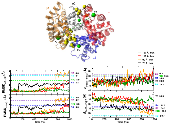
Figure 1: Top: Representation of Hb with the C_α atoms of the residues relevant to Perutz’ stereochemical mechanism shown as yellow spheres. The iron atoms (green spheres) are connected with green dashed lines, indicating the distances reported. Blue, red, grey, and gold ribbon structures for $\alpha_{1}$, $\beta_{1}$, $\alpha_{2}$, and $\beta_{2}$ subunits of Hb. Bottom: Quaternary structure differences of Hb structures found in the simulations, based on the structural comparison of the $\alpha_{1}\beta_{1}$ and $\alpha_{2}\beta_{2}$ subunits. Black, gold, red, and green traces for simulations in the 75 Å, 90 Å, 120 Å, and 150 Å boxes, respectively. Left panels: (top) RMSD of the nonsuperimposed $\alpha_{2}\beta_{2}$ subunit after superimposing the $\alpha_{1}\beta_{1}$ subunit (C_α carbon atoms were used for both superposition and RMSD calculation); (bottom) RMSD of the nonsuperimposed $\alpha_{1}\beta_{2}$ subunit after superimposing the $\alpha_{2}\beta_{1}$ subunit. Right panels: Iron-Iron distances between the $\alpha$s and $\beta$s of each subunit. Horizontal dashed lines indicate the corresponding values from all known Hb structures (T₀, R₂, RR₂, R₃ and R₄).

Other R-state structures, including R₂, RR₂ and R₃, also exist and present intermediate states between T₀ and R₄. The difference between all Hb forms emerges from differences in the position of the $\beta_{2}$-subunit relative to the $\alpha_{1}$-subunit at the switch region²². This can be shown by superimposing the C_α atoms of the $\alpha_{1}\beta_{1}$ dimers and computing the RMSD for the $\alpha_{2}\beta_{2}$ dimer with the T₀ C_α atoms structure as a reference (Figure 1, top panel) for all Hb forms extracted from crystal structures and for the T₀ Hb structure simulated in different water box sizes. The same applies to superimposing the C_α atoms of $\alpha_{2}\beta_{1}$ dimers and computing the RMSD of the nonsuperimposed regions ($\alpha_{1}\beta_{2}$ dimer, and also on the $\alpha$ carbons) with the T₀ structure as a reference point (Figure 1, left bottom panel). And as a measure of quaternary variation, the complete $\alpha_{1}\beta_{1}$ $\alpha_{2}\beta_{2}$ tetramer was superimposed on the C_α atoms (Figure S2) 3rd panel from top). It is found that these different RMSD results follow the same trends when comparing different R forms and box sizes. R₃ shows the most shift and is closest to T₀, followed by RR₂ and lastly by the R₂ and R₃ structures.

Figure 1 also shows that the large quaternary structural difference between the T and R forms is accompanied by significant changes in the $\alpha_{1}$-$\alpha_{2}$ and $\beta_{1}$-$\beta_{2}$ iron-iron distances; they are reduced in the R-states, most notably for the R₃ structure (right panels). This movement of the subunits has a large effect on the interdimer interface (as observed in the interaction distances reported in Figure S3) and thus on the central water cavity relative to the T₀ structure. There is also the change in the C_α-C_α distance between His146$\beta_{1}$ and His146$\beta_{2}$ and the C_α-C_α distance between His143$\beta_{1}$ and His143$\beta_{2}$, as well as the change in the $\theta$ angle between the two planes containing His146$\beta_{1}$-Fe$\beta_{1}$-Fe$\alpha_{1}$ and His146$\beta_{2}$-Fe$\beta_{2}$-Fe$\alpha_{2}$. The angle between the $\alpha_{1}\beta_{1}$ and $\alpha_{2}\beta_{2}$ subunits is smaller in all R-forms compared to the T structure (Figure S2, bottom panel). These values explain the shorter distances between His146$\beta_{1}$ and His146$\beta_{2}$, and between His143$\beta_{1}$ and His143$\beta_{2}$ reported in Figure S2 (first two panels from top). Hence, the $\beta$-cleft entrance to the central water cavity is narrowed (compared to the T₀ structure with the largest central cavity) and this leads to less water entering the central cavity. The decrease in the number of water molecules in the central cavity was noted in our previous paper ⁴ where water molecules present in the central cylinder for the different box sizes were counted (see Figures 5-figure supplement 3 and 4 in Ref.⁴).

Local structural changes around His146 resulting from differences in the position of the $\beta_{2}$-subunit relative to the $\alpha_{1}$-subunit are also observed (Figure S3). In all R forms compared to the T structure, the water-mediated contact (His146$\beta$)COO–OC(Pro37$\alpha$) and the salt bridges between (His146$\beta$)COO–NZ(Lys40$\alpha$) and (His146$\beta$)NE2–COO(Asp94$\beta$) are absent. Further, the salt bridge missing in the T₀ form between (His146$\beta$)COO and NE(His2$\beta$) is observed only in the R₄ form.

Specific H-bonds at the $\alpha_{1}\beta_{2}$ dimer interface involved in the shearing motion were also analyzed (Figure S4). First, the hydrogen bond between Thr38$\alpha_{1}$ and His97$\beta_{2}$, present in the R₃ structure but missing in the RR₂ and R₂ intermediate structures, was sampled in our simulations. Second, the hydrogen bond between Tyr42$\alpha_{1}$ and Asp99$\beta_{2}$ present only in the T₀ structure and absent in all R-forms was observed for the stable T₀ state simulation (150 Å box) and was absent in all boxes with transitions. Finally, the hydrogen bond between Arg92$\alpha_{1}$ and Gln39$\beta_{2}$ or Glu43$\beta_{2}$ present in RR₂ and missing in all other states was observed.

The conformational differences between the T and R states affect the hydration environment in a manner that can be related to $\delta\lambda_{\mathrm{phob}}^{(r)}$. Based on the results of previous simulations⁴, the set of residues for which $\delta\lambda_{\textrm{phob}}$ changes most across the transitions was selected. Figure 2 (top panel) reports the C_α His146$\beta_{1}$–His146$\beta_{2}$ separation, which serves as an indicator of the T-to-R transition for the simulations in the 90, 120, and 150 Å boxes. For the simulations in the two smaller boxes, three red transitions are evident between the T₀-state (at early times) and the R₀-state (at late times, see Figure 1 in Ref.⁴), as indicated by the red dashed lines in Figure 2. Structural changes are accompanied by changes in the number of hydration waters. For the simulation in the largest (150 Å) box, for which no transition occurs, the C_α His146$\beta_{1}$–His146$\beta_{2}$ separation is constant and the average hydration is larger than 0.95 (see bottom row in Figure 2).

(a) Results for Hb 90 Å box: Local hydrophobicity (LH) for residues identified as the Perutz stereochemical model (see Table 1). The LH analysis for the 1 $\mu$s simulation is carried out with a time resolution of 0.5 ns. A cut-off of 6 Å from the protein is chosen to distinguish between interfacial and bulk water. The structural transitions for the 90 Å box occur at $t=470$ ns, $t=770$, and $t=891$ ns, as indicated by the distance $r_{\rm His146}$ between the C_α atoms of the two His146 residues in the $\beta_{1}$ and $\beta_{2}$ chains. The total number of interfacial water is found to correlate with this distance (see bottom row of Figure 2). Whenever the distance between the two His146 residues (see reference ⁴) decreases abruptly (as indicated by the red dashed lines), the relative number of water molecules $r_{w}$ within the 6 Å cut-off increases. The value of $r_{w}=N_{\rm wat}/N_{\rm max}$ was determined as the instantaneous number $N_{\rm wat}$ of water molecules for a specific snapshot and the maximum $N_{\rm max}$ encountered along the entire trajectory.

Figure 2: Top: The C_α His${}_{146}\beta_{1}$–His${}_{146}\beta_{2}$ separation as a function of time for the 90, 120 and 150 Å box from left to right. Raw data in black and running averages over 50 ns in green. The arrows on the right-hand side indicate the His₁₄₆$\beta_{1}$–His₁₄₆$\beta_{2}$ separation ($r_{\rm His146,C\alpha C\alpha}$) in the 2DN2 (T₀) and 2DN3 (R₄) crystal structures.²³ Bottom: The hydration (”H₂O ratio”) of the entire protein, expressed in terms of $r_{w}=N_{\rm wat}/N_{\rm max}$. The vertical red dashed lines indicate the transition times for the three steps observed in the 90 Å and 120 Å boxes (see Figure 1B of reference ⁴.

Table 1: The residues of Hb for which the local hydrophobicity $\delta\lambda_{\textrm{phob}}$ is analyzed from Perutz’ stereochemical model²¹. For each residue its involvement in specific contacts is reported.

Residue	Role in the protein
Arg141$\alpha_{1}$	$\alpha$ C-terminal salt bridge
Val1$\alpha_{2}$	$\alpha$ C-terminal salt bridge
Asp126$\alpha_{2}$	$\alpha$ C-terminal salt bridge
Lys127$\alpha_{2}$	$\alpha$ C-terminal salt bridge
Tyr140$\alpha_{1}$	$\alpha$ proximity to the C-terminal residue
His146$\beta_{1}$	$\beta$ C-terminal salt bridge
Lys40$\alpha_{2}$	$\beta$ C-terminal salt bridge
Asp94$\beta_{1}$	$\beta$ C-terminal salt bridge
Tyr145$\beta_{1}$	$\beta$ salt bridge involved in His146$\beta_{1}$ motion
Val98$\beta_{1}$	$\beta$ salt bridge involved in His146$\beta_{1}$ motion
Thr38$\alpha_{1}$	$\alpha_{1}-\beta_{2}$ shearing
Thr41$\alpha_{1}$	$\alpha_{1}-\beta_{2}$ shearing
Tyr42$\alpha_{1}$	$\alpha_{1}-\beta_{2}$ shearing
Asp94$\alpha_{1}$	$\alpha_{1}-\beta_{2}$ shearing
Cys93$\beta_{2}$	$\alpha_{1}-\beta_{2}$ shearing
Val98$\beta_{2}$	$\alpha_{1}-\beta_{2}$ shearing
Asn102$\beta_{2}$	$\alpha_{1}-\beta_{2}$ shearing
Asp99$\beta_{2}$	$\alpha_{1}-\beta_{2}$ shearing

To obtain more detailed information, $\delta\lambda_{\textrm{phob}}(t)$ was analyzed for the residues listed in Table LABEL:tab:tab1, see Figure 3. For certain residues, structural transitions (at $t=470$ ns, $t=770$ ns, and $t=891$ ns) are accompanied by abrupt rather than by gradual changes in local hydrophobicity of individual residues. Examples include Val98$\beta_{1}$, Thr41$\alpha_{1}$, or Asp94$\alpha_{1}$. By contrast, Tyr42$\alpha_{1}$ shows a gradual decrease in $\delta\lambda_{\mathrm{phob}}$ over most of the 1 $\mu$s simulation. There are also changes in LH away from overall structural transitions, e.g. for Val98$\beta_{2}$, Asp99$\beta_{2}$, and Asn102$\beta_{2}$ at 200 ns, further discussed below. Except for Val98$\beta_{1}$ all residues that show a substantial decrease in their hydrophilic ($\delta\lambda_{\textrm{phob}}\sim 0.5$) versus hydrophobic ($\delta\lambda_{\textrm{phob}}\sim 0$) character [Thr41$\alpha_{1}$, Tyr42$\alpha_{1}$] or an increase [Thr38$\alpha_{1}$, Asp94$\alpha_{1}$, Asp99$\beta_{2}$] are at the $\alpha_{1}/\beta_{2}$ interface. This suggests that the decay for the 90 Å box is triggered primarily by the hydration around residues that are involved in the $\alpha_{1}/\beta_{2}$ contacts.

Based on the data in Figure 3, the T${}_{0}\rightarrow$R₀ transition in the 90 Å box is accompanied by significant changes in the hydration environment at certain locations around the $\alpha_{1}/\beta_{2}$ contact. This observation is consistent with Perutz’ conclusion. We quote, “[..]Where is the force that changes the quaternary structure applied[..]The evidence is overwhelmingly in favor of the contacts $\alpha_{1}\beta_{2}$[..]”.²¹ The significant changes in hydration around the $\alpha_{1}\beta_{2}$ contact suggest the possibility that the T${}_{0}\rightarrow$R₀ transition is driven by solvent thermodynamics.

(b) Results for Hb 120 Å box: For the simulation in the 120 Å box most of the residues involved in the salt bridges, like those in the 90 Å box, show only minor variations in $\Delta\langle\delta\lambda_{\textrm{phob}}\rangle$ except that of Tyr145$\beta_{1}$ and Val98$\beta_{1}$ which have the largest variations along the trajectory (see Figure 4B). It is found that the LHs of all other residues in Figures 3A, B and 4A, B behave similarly in the simulations of the 90 Å and 120 Å boxes. For Val98$\beta_{1}$, instead of decaying to $\Delta\langle\delta\lambda_{\textrm{phob}}\rangle\approx 0$ as in the simulation of the 90 Å box, the value of $\Delta\langle\delta\lambda_{\textrm{phob}}\rangle$ in the 120 Å box remains at or above 0.5 throughout the entire simulation. Hence, the T₀ $\rightarrow$ R₀ transition is again mainly associated with motion at the $\alpha_{1}/\beta_{2}$ interface (see Figure 4C,D). An example of a transition that follows the mechanism described by Perutz²¹ is the transition at 620 ns at the $\alpha_{2}/\beta_{1}$ interface, where the cleavage of the Tyr42$\alpha_{2}$ and Asp99$\beta_{1}$ salt bridge is clearly visible (see Figure S4 middle panel and Figure S5).

Several of the residues at the $\alpha_{1}/\beta_{2}$ interface show pronounced changes in local hydrophobicity that coincide with structural transitions (Figures S3 and S4). However, a few residues in Figure 4D also show LH changes that are not necessarily linked directly to a tertiary structural change (“step”); they are Val98$\beta_{2}$, Asp99$\beta_{2}$, and Asn102$\beta_{2}$ at around 500 ns, further discussed below. For the transitions at 620 ns and 840 ns there is again a clear change in LH for Thr38$\alpha_{1}$, Thr41$\alpha_{1}$, and Asp94$\alpha_{1}$, the most pronounced of them involving Thr38$\alpha_{1}$. These observations also indicate that the nature of the transition at 470 ns (step1) in the 90 Å and at 620 ns (step1) in the 120 Å box is different and may be explained by the transition to different intermediate R-forms (see next paragraph).

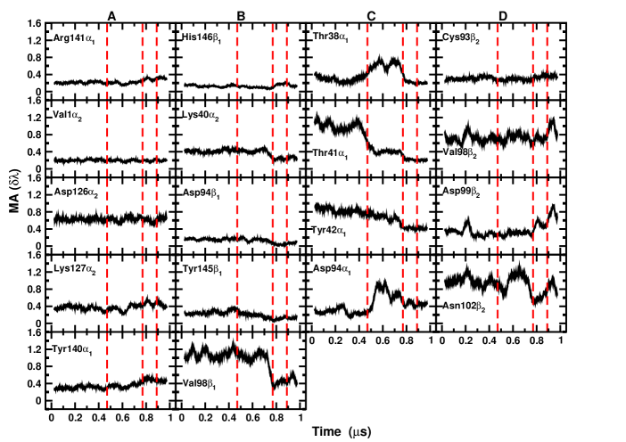
Figure 3: Local hydrophobicity for the simulation in the 90 Å box. Moving average (MA) over 50 ns of $\delta\lambda_{\textrm{phob}}$ as a function of time for residues involved in the C-terminal salt bridges²¹ (column A), additional salt bridges (column B) and the $\alpha_{1}\beta_{2}$ (columns C and D); see Table LABEL:tab:tab1.

For the decaying structures in the 90 Å and 120 Å boxes the following is observed. In the 90 Å box, a transition from T₀ to R₃ starts at 470 ns (step1), where the His146–His146 separation drops from 31 Å to 25 Å bringing the Hb structure closer to R₃ (22 Å, Figure S2, first panel). This T₀ to R₃ transition is completed at 780 ns (step2, Figure S2, the presence of the R₃ structure at 780 ns is marked in all the panels by a cyan dashed line). At $\sim 880$ ns (step3) a next transition from R₃ to R₂ occurs (the R₂ structure is marked by a violet dashed line in Figure S2). For the rest of the simulation until 1 $\mu$s, the RR₂ and R₄ states are sampled (Figure S2, RR₂ and R₄ states are indicated by a green dashed line and a blue arrow, respectively). Conversely, in the 120 Å box, at step1 at 620 ns a T₀ to R₂ transition starts by decaying to an unknown intermediate. It is continued at 840 ns (step2) to bring the structure closer to R₂. The transition to R₂ is completed by 920 ns (step3, Figure S2), the presence of the R₂ structure at 920 ns is indicated in all the panels by a vertical violet dashed line).

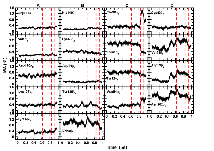
Figure 4: Local hydrophobicity for the simulation in the 120 Å box. Moving average [MA ($\delta\lambda$)] over 50 ns of $\delta\lambda_{\textrm{phob}}$ as a function of time for residues involved in the C-terminal salt bridges²¹ (column A), additional salt bridges (column B) and the $\alpha_{1}\beta_{2}$ shearing motion (columns C and D); see Table LABEL:tab:tab1. The presence of the R₂ structure at 920 ns is indicated in all the panels by a vertical violet dashed line.

(c) Results for Hb 150 Å box: For the 150 Å box the previous MD simulations did not find a structural transition.⁴ The values of $\delta\lambda_{\textrm{phob}}$ for all residues involved in the salt bridges (Figure 5, columns A and B) do not deviate significantly from their average value. The amplitude of the fluctuations are typically smaller than for the simulations in the 90 Å and 120 Å boxes. For the residues at the $\alpha_{1}\beta_{2}$ interface there are variations for Thr38$\alpha_{1}$, Thr41$\alpha_{1}$, Tyr42$\alpha_{1}$, and Asp94$\alpha_{1}$ (see Figure 5).

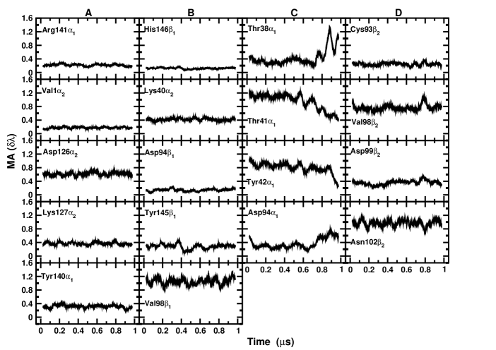
Figure 5: Local hydrophobicity for the simulation of the 150 Å box. It shows moving averages over 50 ns of $\delta\lambda_{\textrm{phob}}$ as a function of time for residues involved in the C-terminal salt bridges²¹ (column A), additional salt bridges (column B) and the $\alpha_{1}\beta_{2}$ shearing motion (columns C and D), see Table LABEL:tab:tab1.

The clearest difference between the simulation in the 150 Å and the two smaller boxes is the behaviour for residues Val98$\beta_{2}$, Asp99$\beta_{2}$, and Asn102$\beta_{2}$. As an example, the water occupation around Val98$\beta_{2}$ is analyzed by computing the radial distribution function $g(r)$ between the C_α of the residue and the surrounding hydration water for different parts of the trajectory. The radial distribution functions $g(r)$ in Figure S6 show that they are close in shape to one another but differ in magnitude for the early phase of the trajectory in the 120 Å and 150 Å box. They change in shape after the transition at 840 ns in the smaller of the two boxes. A pronounced signature in LH is also found in the 120 Å and 150 Å boxes for Thr38$\alpha_{1}$ between 800 and 900 ns. The signatures in LH for the 150 Å box can be related to formation of a Thr38$\alpha_{1}$–Asp99$\beta_{2}$ salt bridge (Figure S7). Breaking and reforming of salt bridges involving Val98$\beta_{2}$, Asp99$\beta_{2}$, and Asn102$\beta_{2}$ is also responsible for the sharp increase in LH around these three residues in the 90 Å box around 200 ns, see Figures 3D and S8. It is notable that the LH around the three residues already starts to change before the salt bridge actually breaks.

Changes of the LH of each residue can be due to a) internal motion of a residue or b) the influence of neighbouring residues. Both of these are potentially followed by water displacement or influx which change $\delta\lambda_{\rm phob}$. For the transition at $t=840$ ns in the 120 Å box, changes in the local water occupation around Val98$\beta_{2}$ obtained by analysis of radial distribution functions (see Figure S6) do not necessarily lead to changes in LH. The $g(r)$ for the time intervals 0 to 620 ns and 620 ns to 840 ns are very similar (red and green lines in Figure S6) while the LH changes from 0.8 at early times to 1.2 after $t\sim 500$ ns, see Figure 4. The water influx is a consequence of the reconfiguration of the H-bonding network including the Tyr42$\alpha_{1}$–Asp99$\beta_{2}$ salt bridge (see Figure S9) and the rearrangement of the carboxy group of the sidechain of Asp99$\beta_{2}$ due the rehydration of the side chain. These effects are also mirrored by the Asp99$\beta_{2}$ carboxy orientation (see dihedral time series reported in Figure S11) which demonstrates that before the transition at 840 ns the side chain follows a two-state behaviour but after the transition almost free rotation occurs (see also Figure S4). This change is accompanied by increased hydration of the side chain (bottom panel of Figure S11).

Comparing Figures 3 to 5 it is noted that even when Hb is still in its T₀ state (i.e. before 470 ns, the first transition in the 90 Å box), differences in LH, mainly at the $\alpha_{1}/\beta_{2}$ interface are observed. Examples include residues Thr41$\alpha_{1}$ and Tyr42$\alpha_{1}$ for which LH oscillates or decreases in the 90 Å box but remains constant in the two larger boxes before 470 ns. The finding that destabilization of the $\alpha_{1}/\beta_{2}$ interface is at the origin of the T₀ to R₀ transition is consistent with the Perutz stereochemical model. Conversely, the LH around the C-terminal salt bridge residues is very similar for the simulations in the three different box sizes, except for Val98$\beta_{1}$ and Tyr145$\beta_{2}$.

(d) Spatio-temporal analysis based on two-dimensional correlation maps: To better understand the coupling of local hydration dynamics and the structural transitions, two-dimensional correlation maps were generated which are referred to as local hydrophobicity cross correlation maps (LH-CCMs). Similar to dynamic cross correlation maps (DCCMs)^{24, 25} for residues $i$ and $j$ the quantity

$$C_{ij}=\frac{\langle\Delta\delta\lambda_{\textrm{phob}}^{(i)}\Delta\delta\lambda_{\textrm{phob}}^{(j)}\rangle}{\sqrt{\langle(\Delta\delta\lambda_{\textrm{phob}}^{(i)})^{2}\rangle\langle(\Delta\delta\lambda_{\textrm{phob}}^{(j)})^{2}\rangle}}$$ (2)

was determined for each interval for which Hb was in a particular conformational state as shown in Figure 1.

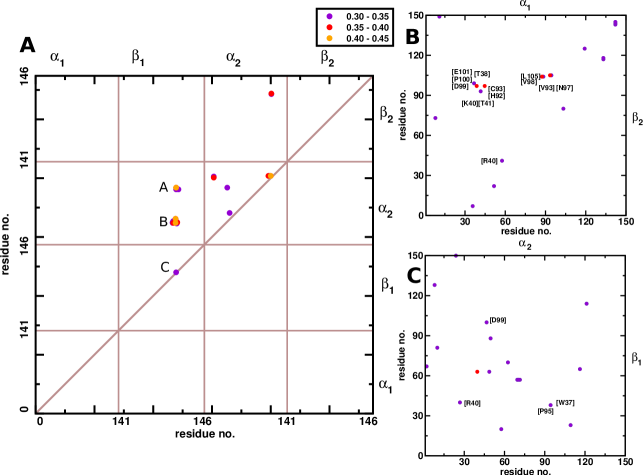
Figure 6: Difference of Local Hydrophobicity $\Delta C_{ij}$ Cross Correlation Map (LH-CCM) for the 120 Å box. Panel A: difference between [0-620] and [620-840], i.e. ”transition at 620” for entire protein. Panel B: difference between [620-840] and [840-920], i.e. ”transition at 840” for the $\alpha 1/\beta 2$ interface. Panel C: difference between [620-840] and [840-920], i.e. ”transition at 840” for the $\alpha 2/\beta 1$ interface. The cross correlations for the individual states are given in Figure S12. Only values $\Delta C_{ij}\geq 0.30$ are reported. Color code: $0.30\leq\Delta C_{ij}<0.35$ (purple), $0.35\leq\Delta C_{ij}<0.40$ (red), and $0.40\leq\Delta C_{ij}<0.45$ (orange).

Figure 6A reports the difference between the local hydrophobicity cross correlation maps between time intervals 0 to 620 ns and 620 to 840 ns for the 120 Å box for values of $\Delta C_{ij}>0.3$. This map indicates that correlations in LH and their difference can depend on both the sequence and spatial proximity of two residues. The correlation in LH up to 620 ns (i.e. before the first transition, see Figure S10) is large ($C_{ij}>0.30$) for residues that play an active role in interface transitions between the two subunits (Figure 6 above the diagonal) and for regions that are spatially close (on the diagonal). An example for sequence proximity is the Val98$\beta_{1}$-Asp$99\beta_{1}$ region (feature C in Figure 6A and Figure S9). Changes in LH are a direct consequence of the Asp99$\beta_{1}$-Tyr42$\alpha_{2}$ salt bridge cleavage during the transition at 620 ns (see Figure S5) that leads to a change in the orientation of the peptide bond between Val98$\beta_{1}$-Asp$99\beta_{1}$ (Figure S9) and corresponding decrease in the LH of both, Asp99$\beta_{1}$ and Tyr42$\alpha_{2}$. Examples for spatial proximity of residues are the two clusters (labelled A and B in Figure 6A) that are at the $\alpha_{2}\beta_{1}$ shearing interface. This change in hydrophobicity in one of the two important stabilizing regions of the protein (the other being the $\alpha_{1}/\beta_{2}$ interface), indicates its possible involvement in the destabilization of the T₀ structure.

A more detailed view of the LH cross correlations for the $\alpha_{1}\beta_{2}$ interface for the 120 Å box is provided in Figure S10 (for LH-CCMs in the 90 Å and 150 Å boxes see Figures S13 and S14). Figure S10 shows the LH cross correlations for residues involved in the $\alpha_{1}/\beta_{2}$ shearing motion up to 620 ns. The clusters (A to E) in Figure S10 involve correlated changes in LH at the $\alpha_{1}$/$\beta_{2}$ interface, whereas for cluster F no direct contact is present. In cluster A the correlation is caused by the Thr41$\alpha_{1}$–Arg40$\beta_{2}$ salt bridge present before the transition at 620 ns. Cluster B is dominated by the water-mediated Asp94$\alpha_{1}$–Arg40$\beta_{2}$ salt bridge before the transition at 620 ns; it is a weak interaction due to the large distance ($\sim 6$ Å) between the proton and the anion. After the transition this salt bridge becomes the dominant interaction in which Arg40$\beta_{2}$ is involved. The C cluster is dominated by the $\pi$-stacking interaction between Tyr140$\alpha_{1}$ and Trp37$\beta_{2}$. A weak salt bridge of the Thr38$\alpha_{1}$ and Asp99$\beta_{2}$ sidechains with the Thr41$\alpha_{1}$ sidechain and Asp99$\beta_{2}$ NH peptide bond are responsible for the D cluster. The NH peptide bond of Asn97$\alpha_{1}$ and the Asp99$\beta_{2}$ side chain lead to cluster E. Overall, this figure provides a dynamic view of the stereochemical model proposed by Perutz.²¹ This is illustrated, for example, by the fact that all clusters (A to F) are extended, rather than the usual point-to-point contacts (i.e., the salt bridges) alone.

Next, the transition in the 120 Å box at 840 ns is discussed from the perspective of the LH-CCMs (see Figure 6 panels B and C). They show the difference between the LH-CCMs for the time intervals [620-840] ns and [840-920] ns, respectively. During the process two salt bridges are broken (Thr41$\alpha_{1}$–Asp99$\beta_{2}$ and Thr41$\alpha_{1}$-Arg40$\beta_{2}$, which is water mediated) and two new salt bridges are formed (Thr38$\alpha_{1}$–Asp99$\beta_{2}$ and Asp94$\alpha_{1}$–Arg40$\beta_{2}$) and Asn97$\alpha_{1}$ - Asp99$\beta_{2}$ continues to show a bimodal behaviour, see Figure S15. It is found that the reformation of these salt bridges between residues involved in the “Perutz mechanism” (Thr38$\alpha_{1}$, Thr41$\alpha_{1}$, Asp94$\alpha_{1}$ and Asp99$\beta_{2}$) is also reflected in the difference cross correlation maps (Figure 6B and C). They confirm that most of the changes for this transition occur at the $\alpha_{1}/\beta_{2}$ interface. Also, these two panels show that changes in the LH-CCMs are not necessarily symmetric for the $\alpha_{1}/\beta_{2}$ and $\alpha_{2}/\beta_{1}$ interfaces. Such a “dynamical asymmetry” (i.e., it is found in the molecular dynamics simulations) has also been observed for insulin dimer²⁶ for which the X-ray structure has C₂ symmetry²⁷ or is very close to symmetric with only small local deviations from it.²⁸

As previous results have shown, the relative stability of the T₀ state depends on the size of the simulation cell.⁴ Analysis of hydration structure via $\delta\lambda_{\mathrm{phob}}^{(r)}$ has the ability to reveal when and where protein hydration properties differ between differently sized simulation cells. To highlight this point, the statistics and dynamics of $\delta\lambda_{\mathrm{phob}}^{(r)}$ for Hb in the T₀ state in the 90 Å and 150 Å simulation boxes are compared in Figure 7. It summarizes the values of $\delta\lambda_{\mathrm{phob}}^{(r)}$ over the residues that comprise the $\alpha_{1}/\beta_{2}$ and $\alpha_{2}/\beta_{1}$ interfaces, as a function of simulation time. Most notably, as the conformational transition from the $T_{0}$ state to the $R_{0}$ state progresses, there is a distinct shift towards values of $\delta\lambda_{\mathrm{phob}}^{(r)}$ near zero. This indicates that the interfacial water structure shifts from that observed at a hydrophilic surface towards that observed at a hydrophobic surface (Figure 7A). The shift in interfacial water structure is also apparent from the probability distribution, $P(\delta\lambda_{\mathrm{phob}}^{(r))})$, for the different simulation box sizes. During the first 500ns of the trajectories the probability distributions overlap (Figure 7B), showing that the interfacial water structure does not differ significantly. However, during the last 500 ns of the trajectories the probability distribution for the 90Å simulation box has a significant shift towards lower values of $\delta\lambda_{\mathrm{phob}}^{(r)}$, corresponding to a more hydrophobic character of the interface (Figure 7C).

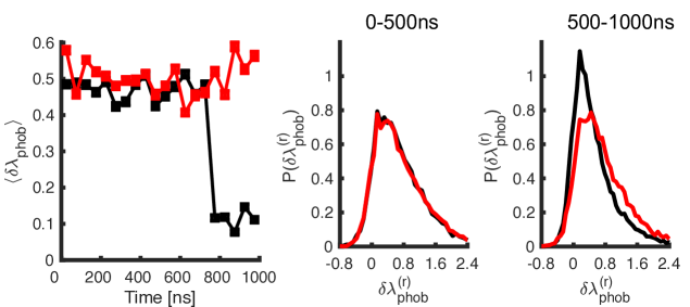
Figure 7: Comparison of the interfacial water structure for residues that are part of the $\alpha_{1}/\beta_{2}$ and $\alpha_{2}/\beta_{1}$ interfaces. The black and red lines correspond to simulations carried out in $90\mathrm{\AA}$ and $150\mathrm{\AA}$ solvent boxes, respectively. The marker indicates the center of a time interval. Panel A: The expectation value of $\delta\lambda_{\mathrm{phob}}^{(r)}$ as a function of time, averaged over 50 ns time intervals. Panel B: The distribution of $\delta\lambda_{\mathrm{phob}}^{(r)}$ values during the first 500 ns of the trajectories. Panel C: The distribution of $\delta\lambda_{\mathrm{phob}}^{(r)}$ values during the last 500 ns of the trajectories.

3.2 Hydration Dynamics around Melittin

As a second example, the analysis of water hydration for Hb has been extended to melittin. It is a well studied prototype of a protein complex that is stabilized through hydrophobic interactions. Melittin is a small, 26-amino acid protein (for the sequence, see Figure S16) found in honeybee venom that crystallizes as a tetramer, consisting of two dimers (see Figure 8 left), related by a two-fold symmetry axis.^{8, 9} Cheng and Rossky⁷ characterized the behaviour of the hydrophobic surface of the melittin dimer and of the surrounding surface residues by simulations in which the structure of the melittin dimer was frozen. They found that in hydrophilic regions the water molecules have a well defined orientation, while in the hydrophobic regions, the waters are more mobile and explore different configurations.⁷ To further explore the hydration dynamics, simulations with a frozen melittin dimer in different box sizes are carried out and analyzed. In additional simulations, the protein was also allowed to move freely. These provide information about the solvent-solute coupling.

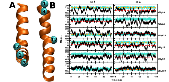
Figure 8: Left: A- and B-helices with the Gly1, Gly3, and Gly12 residues represented as spheres. The A-helix is slightly bent at the C-terminal end for the rigid and flexible simulations. The RMSD of the two chains of the dimer is 1.6 Å. Right: Time evolution of $\delta\lambda_{\textrm{phob}}$ for the 6 glycine residues in the melittin dimer. The results of the simulations for the rigid (cyan) and flexible (black) protein are reported. The orange and red line represent the average $\delta\lambda_{\textrm{phob}}$ for each residue during the simulation. Gly12 is less hydrophilic than the other Gly residues since it is located in the hydrophobic region of the protein.

It is of interest to analyze whether $\delta\lambda_{\rm phob}$ encapsulates corresponding information, and whether simulations of water around a rigid melittin dimer, as carried out in Ref.⁷, and around a flexible dimer lead to qualitatively similar results. Since the results for Hb depend on the box size, simulations are also carried out with different box sizes.

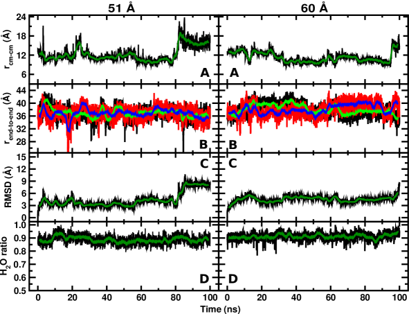
Figure 9: Flexible melittin in the 51 Å and 60 Å boxes. In Panels A the center-of-mass distance between the two monomers ($r_{\textrm{cm-cm}}$) is reported as function of time (black: raw data; green: moving average). Around 80 ns, a rearrangement of the two monomers is associated with an increase of $r_{\textrm{cm-cm}}$. The chain length ($r_{\textrm{end-to-end}}$) for the two segments (black and red for the raw data for chain A and B, green and blue for their moving average), are illustrated in Panels B. The RMSD with respect to the initial structure of the protein is shown in Panels C. During the time evolution, the number of water surrounding the protein seems not to be influenced by the structural changes as shown in Panels D.

The structural variations together with the overall hydration of the flexible melittin dimer in the different water box sizes are reported in Figure 9. In all simulations the end-to-end separation of the two helices (see Figure 9B) as defined by the C_α-C_α separation of the two terminal residues Gly1 and Gln26 is stable, indicating that the helices (the H₂O ratio) remain intact. Consequently, the structural transition that occurs after 80 ns in the 51 Å box (Figure 9C) and appears to occur towards the end of the simulation in the 60 Å box involves the dimerization interface. This is confirmed by panel A, which reports an increase of the center-of-mass distance $r_{\textrm{cm-cm}}$ between the two helices at the same time as the RMSD in panel C increases. The degree of hydration (Figure 9D) defined as $r_{w}=N_{\rm wat}/N_{\rm max}$ remains essentially constant throughout the simulations.

The protein-water interface is analysed using the same methodology as that used for Hb. The Willard-Chandler interface is calculated setting $r_{\rm cut}=25.0$ Å and the likelihood ($\delta\lambda_{\textrm{phob}}$) of the interfacial water with the reference TIP3P water model is determined with a 6 Å cut-off. Figures 8 and S17 show the time evolution of selected residues. Figure 8 shows the temporal evolution, $\delta\lambda_{\textrm{phob}}$, of glycine residues Gly1, Gly3, and Gly12 for chains A and B for both the rigid and the flexible dimers. The $\delta\lambda_{\textrm{phob}}$ for the rigid dimer is essentially constant, as expected. The results reported are all averages over 2 ns windows.

Table 2: Average $\delta\lambda_{\textrm{phob}}$ for the glycine residues for the 100 ns simulation (see Figure 8).

Residue	51 Å flexible	51 Å rigid	60 Å flexible	60 Å rigid
1A	1.068	1.583	0.989	1.598
3A	1.090	1.604	0.983	1.616
12A	0.965	0.882	0.979	0.945
1B	1.192	1.614	0.921	1.587
3B	1.156	1.584	0.927	1.568
12B	0.917	0.799	0.968	0.826

For the rigid monomer (blue traces in Figure 8) the LH is constant along the entire 100 ns simulation for both box sizes and the averages differ by 10 % at most (Gly12A). For the flexible dimer (black traces) the instantaneous LH fluctuates around well-defined average values except for Gly12B which has a slight increase in its dynamics during the early phase of the simulation, particularly in the 60 Å box. In the simulation in both box sizes the amplitude of LH fluctuates between 0 and 1.6, i.e. between being hydrophobic and hydrophilic. Since Gly is an aliphatic/neutral residue, the changing hydrophilicity must be a consequence of its embedding along the peptide chain and the water structuring around it. Overall, it is found that Gly12A and 12B, which are near the middle of the helix, are less hydrophilic (see Figure 8 and Table 2) than Gly1 and Gly3, which are positioned at or near the terminus. This difference is more pronounced for the rigid dimer.

Figure S17 shows the LH for the residues investigated by Cheng and Rossky⁷ for the 51 Å box while those for the 60 Å box are given in Figure S18. The average $\delta\lambda_{\textrm{phob}}$ are neutral or hydrophilic. Good qualitative agreement with Ref⁷ is found for residues Val8A (hydrophilic), Leu9A, Ile13A, Ile13B (residues with a decreasing level of hydrophobicity), and Ile20B.

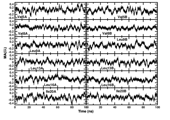
Figure 10: Difference in hydrophobicity for the residues in the melittin dimer hydrophobic pocket as defined in Ref. ⁷ for the rigid simulations in the 51 and 60 Å boxes. They are residues Val5, Val8, Leu13, Leu16, Ile20. The data reported is $\Delta\delta\lambda=\delta\lambda_{60}-\delta\lambda_{51}$, i.e. the change in LH from the simulation in the two water boxes. The maximum instantaneous change in $\Delta\delta\lambda_{\textrm{phob}}$ due to the box size is 40 %; most differences are 20 % or less.

It is also of interest to compare the difference in hydrophobicity for simulations of rigid melittin in the two water boxes because all differences must arise from the size of the water box. Figure 10 shows the difference between the 51 Å and the 60 Å boxes in LH of the residues in the hydrophobic pocket. The average fluctuations are of the order of 0.1 units with maximum differences of 0.4 units. The difference between simulations with rigid and flexible melittin can also be seen when comparing the radial distribution functions, $g(r)$, between C_α atoms of selected residues and water and the corresponding water occupations $N(r)$ (see Figures S19 and S20). The residues were chosen in accord with the results from Table 3. For example, in the 51 Å box for rigid melittin the values for Val5A and Val5B are $\delta\lambda_{\rm phob}=1.19$ and 1.48, respectively, which change to 1.25 and 1.49 in the larger 60 Å box; i.e., this is a change of 5 % at most. Figure S19A shows that $g(r)$ for Val5A and Val5B are very similar for both water box sizes. This suggests that the difference of $\sim 0.25$ in Table 3 for the two water boxes must arise from the orientation of the water molecules within the 6 Å cut-off.

Conversely, for flexible melittin the differences for LH in the two water boxes can be substantial. As an example, Leu9B $\delta\lambda_{\rm phob}^{\rm 51A}=0.81$ is compared with $\delta\lambda_{\rm phob}^{\rm 60A}=1.07$ for the two box sizes. This is also evident from Figure S20A and B (right panel) for which $g(r)$ and $N(r)$ have increased amplitudes for the larger water box. For Val5B, $\lambda_{\rm phob}^{\rm 51A}=1.05$ is larger in the smaller box than $\lambda_{\rm phob}^{\rm 60A}=0.86$, whereas the amplitude of $g(r)$ up to the 6 Å cut-off in the larger box is larger than that in the smaller box. Hence, the difference found in the two box sizes must arise from the angular orientations of the water molecules relative to the protein surface. These analyses suggest that both the distance-dependence (reflected in $g(r)$ and $N(r)$) and the angular orientation, as measured by $\lambda_{\rm phob}$, can depend on box size and potentially influence the thermodynamic stability of the two proteins.

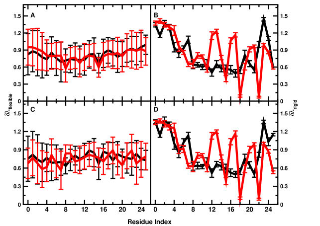
Figure 11: Average $\delta\lambda_{\rm phob}$ per residue for the 100 ns simulation for chains A (black) and B (red) for the flexible (panels A and C) and the rigid (panels B and D) melittin dimer. The top row is for the 51 Å box and the bottom row for the 60 Å box. The value of the LH ranges from $0.50<\delta\lambda_{\rm phob}<1.00$ for the flexible dimer and between $0.00<\delta\lambda_{\rm phob}<1.50$ for the rigid dimer. For the rigid dimer, the central part of the A-helix has consistently lower values of LH compared with the C- and N-terminal parts. For chain B larger variations in LH are found for some of the residues due to its different structure. The periodicity of the red traces (panels B and D) reflects the helical structure which is apparent for monomer B but less so for monomer A. For flexible melittin the variation of LH along the sequence is much smoother than for rigid melittin as a consequence of dynamical averaging.

The average hydrophobicity for each residue during the simulation is reported in Figure 11A (black for chain A and red for chain B). The decreased hydrophobicity of the central part of the chains (from Val5 to Leu16) is highlighted by the lower $\delta\lambda_{\rm phob}$ (of 0.1-0.2 units) compared with the C- and N-terminal parts. The main difference between the simulation results for the flexible (left) and rigid (right) melittin dimer is the amplitude of the fluctuation of the hydrophobicity, but not its sign. Simulations of rigid melittin in the 51 Å (panels A and B) and 60 Å boxes (panels C and D) are similar to one another but they differ along the trajectory by up to $\Delta\delta\lambda\sim 0.4$ (see Figure 10). There are also differences between the A (black) and B chains (red) for rigid melittin. The difference in the monomer structures (RMSD of 1.6 Å) leads to significant differences in $\delta\lambda$ (see Figures 11A and B. As an example, Leu13A is considerably more hydrophobic ($\delta\lambda_{\textrm{Leu13A}}=0.7$) than Leu13B ($\delta\lambda_{\textrm{Leu13B}}=1.4$). Inspection of the dimer structure shows that Leu13A points toward the dimerization interface whereas Leu13B points away from it into the solvent. For flexible melittin (panels A and C), the LH for the A and B chains are more similar to one another for both box sizes. This is a consequence of averaging along the structural dynamics. It also suggests that simulations on the 100 ns time scale are sufficient to converge $\delta\lambda$ for melittin. Nevertheless, there remain certain differences between simulations in the two water boxes for individual residues, e.g. $\langle\delta\lambda_{\textrm{Val5B}}^{51}\rangle=1.05$ vs. $\langle\delta\lambda_{\textrm{Val5B}}^{60}\rangle=0.86$, see Figure 11 and Table 3.

Table 3: Average $\delta\lambda_{\textrm{phob}}$ for the hydrophobic residues from Figure 1 in Ref.⁷. The time series are shown in Figure S17

Residue	51 Å flexible	51 Å rigid	60 Å flexible	60 Å rigid
Val5A	0.976	1.185	1.003	1.246
Val8A	0.929	1.322	0.941	1.375
Leu9A	0.954	0.875	0.889	0.876
Leu13A	0.967	0.741	1.030	0.756
Leu16A	0.909	0.808	0.917	0.824
Ile20A	1.019	1.049	1.071	0.992
Val5B	1.046	1.484	0.861	1.494
Val8B	1.038	0.889	0.806	0.877
Leu9B	0.814	0.900	1.071	0.867
Leu13B	1.016	1.393	1.006	1.373
Leu16B	0.835	0.637	1.012	0.626
Ile20B	1.087	0.845	0.988	0.824

Finally, the two-dimensional LH-CCM (see Figure S21) for all four systems and their differences between rigid and flexible dimer (bottom row of Figure S21) have been determined. As can be anticipated from Figure 10, the LH cross correlation maps for the two box sizes are similar for rigid melittin dimer (see Figure S22 left panel). On the other hand, the differences between rigid and flexible melittin dimer in the two boxes are considerably larger, as the bottom row of Figure S21 demonstrates. While for the 51 Å box differences primarily occur at the interface (upper left quadrant), differences for the larger 60 Å box occur both at the interface and along the two helices. Furthermore, the amplitude of the differences increases in going from the 51 Å to the 60 Å box.

The difference between flexible melittin dimer in the 51 Å and 60 Å boxes is shown in Figure S22, right panel. Increasing the box size leads to more pronounced cross correlation peaks between the beginning of helix A and the end of helix B. A slightly less pronounced increase in the correlation is found for the end of chain A and the beginning of chain B. Corresponding radial distribution functions are reported in Figure S23. Even for rigid melittin in the 51 Å (red) and 60 Å (blue) boxes (e.g. for Gly3A and Gln26B) there are slight differences between the $g(r)$. Compared with rigid melittin, the $g(r)$ for flexible melittin are all less structured. Except for Ile2B they also agree well for the two box sizes.

For the rigid and flexible dimer, differences for the two box sizes also occur as shown in the $\Delta$CCC map (Figure S22). They effect the local hydrophobicity which is computed from the water structuring. For the rigid protein surface the differences are essentially independent of box size, as shown in the left panel. For the flexible dimer there are significant differences. They arise both from protein structural changes and the surrounding water structuring. In this context it is interesting to note that $g(r)$ around Leu9A and Leu9B in Figure S20 in the 60 Å box are virtually identical, whereas the LH differs by almost 15 % (0.89 vs. 1.07, see Table 3). As LH includes both the distance between the water oxygen atom relative to the protein surface and the angular orientation of the OH vector, this difference in LH is likely to be related to different orientations of the water network around Leu9A and Leu9B.

4 Conclusions

The present work analyzed the local hydrophobicity around key residues at the protein interfaces for hemoglobin and melittin. It was found that the local hydrophobicity measure for Hb provides valuable insight into the effect of different box sizes from MD simulations. Specifically, analysis of the local hydrophobicity cross correlation coefficients for Hb provided a dynamical view of Perutz’s stereochemical model involving breaking and formation of salt bridges at the $\alpha_{1}/\beta_{2}$ and $\alpha_{2}/\beta_{1}$ interfaces. Also, the more detailed analysis of the simulations in the 90 Å and 120 Å boxes demonstrates that they decay to known but different intermediate structures upon destabilization of the $\alpha/\beta$ interface following a decrease in LH, i.e. as a consequence of reduced water density or change of water orientation at the protein/water interface. This is consistent with earlier findings⁴ that reported a reduced number of water-water hydrogen bonds for the smaller boxes, which influences the equilibrium between water-water and water-protein contacts and hence the water activity. The present results also support recent extensive simulation studies of the A$\beta$ peptide which show that the hydrophobic surface area increases significantly in small cells along with the standard deviation in exposure and backbone conformations.²⁹ As is also reported here (see Figure 7), hydrophilic exposure was found to dominate in large boxes whereas hydrophobic exposure is prevalent in small cells. This suggests there is a weakening of the hydrophobic effect in smaller water box sizes.

Early experiments indicate that T₀ is significantly ($\sim 8$ kcal/mol, equivalent to $K_{\frac{T_{0}}{R_{0}}}=6.7\times 10^{5}$) more stable than R₀.¹ Also, the rate for the R₀ $\rightarrow$ T₀ has been determined as $15700\pm 700$ s^-1 at 303 K, corresponding to a transition time of $\sim 20$ $\mu$s.³⁰ As shown in Ref. ³¹ this implies that the T₀$\rightarrow$R₀ transition occurs on a time scale of 1 to 10 s by use of the Arrhenius equation. This is far too long to be sampled directly by MD simulations with explicit solvent in a statistically meaningful way. As an example, for association free energies in protein-ligand and protein-protein interactions from replica exchange coarse grained simulations, a total simulation time of $>5$ $\mu$s was deemed necessary for convergence³² and similar studies were carried out for protein-ligand interactions using atomistic force fields.^{33, 34} Alternative approaches, such as conjugate peak refinement, string methods, or nudged elastic band in explicit solvent are also ways to more quantitatively investigate the transition state region.^{35, 36, 37} However, to quantify differences between the T₀ and R₀ structure or structures evolving towards the R₀ state (as done here), explicit knowledge of the transition state region is not required.

For the melittin dimer the role of box size on the hydration dynamics was expected to be smaller, based on earlier work on the hydrophobic effect.³⁸ Nevertheless, the analysis of rigid melittin dimer, which was studied in previous work,⁷ suggests that the water distribution is affected by the box size for the 51 Å and 60 Å boxes. These differences become more pronounced when the protein structure is allowed to change in the simulations.

Complementary to radial distribution functions $g(r)$, the local hydrophobicity (LH) provides a time-dependent quantitative local measure characterizing the water dynamics and structure around a protein. When combined with time-dependent structural information a more complete picture for the coupled protein-water dynamics emerges. It provides valuable information about thermodynamic manifestations of structural changes at a molecular level.

Data and Code Availability

The water-structure analysis code used to calculate $\delta\lambda_{phob}$ is publicly available at https://github.com/mjmn/interfacial-water-structure-code.

References

- Edelstein 1971 Edelstein, S. Extensions of allosteric model for haemoglobin. Nature 1971, 230, 224–227
- Hub et al. 2010 Hub, J. S.; Kubitzki, M. B.; de Groot, B. L. Spontaneous Quaternary and Tertiary T-R Transitions of Human Hemoglobin in Molecular Dynamics Simulation. PLoS Comput Biol 2010, 6, e1000774
- Yusuff et al. 2012 Yusuff, O. K.; Babalola, J. O.; Bussi, G.; Raugei, S. Role of the Subunit Interactions in the Conformational Transitions in Adult Human Hemoglobin: An Explicit Solvent Molecular Dynamics Study. J. Phys. Chem. B 2012, 116, 11004–11009
- El Hage et al. 2018 El Hage, K.; Hedin, F.; Gupta, P. K.; Meuwly, M.; Karplus, M. Valid molecular dynamics simulations of human hemoglobin require a surprisingly large box size. eLife 2018, 7, e35560
- Gapsys and de Groot 2019 Gapsys, V.; de Groot, B. L. Comment on ‘Valid molecular dynamics simulations of human hemoglobin require a surprisingly large box size’. eLife 2019, 8, e44718
- El Hage et al. 2019 El Hage, K.; Hedin, F.; Gupta, P. K.; Meuwly, M.; Karplus, M. Response to comment on ‘Valid molecular dynamics simulations of human hemoglobin require a surprisingly large box size’. eLife 2019, 8, e45318
- Cheng and Rossky 1998 Cheng, Y.; Rossky, P. Surface topography dependence of biomolecular hydrophobic hydration. Nature 1998, 392, 696–699
- Terwilliger and Eisenberg 1982 Terwilliger, T. C.; Eisenberg, D. The structure of melittin. I. Structure determination and partial refinement. J. Biol. Chem. 1982, 257, 6010–6015
- Terwilliger and Eisenberg 1982 Terwilliger, T. C.; Eisenberg, D. The structure of melittin. J. Biol. Chem. 1982, 257, L6015
- Shin and Willard 2018 Shin, S.; Willard, A. P. Characterizing Hydration Properties Based on the Orientational Structure of Interfacial Water Molecules. J. Chem. Theor. Comput. 2018, 14, 461–465
- Brooks et al. 2009 Brooks, B. R. et al. CHARMM: The Biomolecular Simulation Program. J. Comput. Chem. 2009, 30, 1545–1614
- Best et al. 2012 Best, R. B.; Zhu, X.; Shim, J.; Lopes, P. E. M.; Mittal, J.; Feig, M.; MacKerell, A. D., Jr. Optimization of the Additive CHARMM All-Atom Protein Force Field Targeting Improved Sampling of the Backbone phi, psi and Side-Chain chi(1) and chi(2) Dihedral Angles. J. Chem. Theor. Comput. 2012, 8, 3257–3273
- Anderson et al. 1980 Anderson, D.; Terwilliger, T. C.; Wickner, W.; Eisenberg, D. Melittin forms crystals which are suitable for high resolution X-ray structural analysis and which reveal a molecular 2-fold axis of symmetry. J. Biol. Chem. 1980, 255, 2578–2582
- Essmann et al. 1995 Essmann, U.; Perera, L.; Berkowitz, M. L.; Darden, T.; Lee, H.; Pedersen, L. G. A smooth particle mesh Ewald method. J. Chem. Phys. 1995, 103, 8577–8593
- Huang et al. 2017 Huang, J.; Rauscher, S.; Nawrocki, G.; Ran, T.; Feig, M.; de Groot, B. L.; Grubmueller, H.; MacKerell, A. D., Jr. CHARMM36m: an improved force field for folded and intrinsically disordered proteins. Nat. Meth. 2017, 14, 71–73
- Swope et al. 1982 Swope, W.; Anderson, H.; Berens, P.; Wilson, K. A Copmuter-Simulation Method for the Calculation of Equilibrium-Constants for the Formation of Physical Clusters of Molecules - Application to Small Water Clusters. J. Chem. Phys. 1982, 76, 637–649
- Hoover 1985 Hoover, W. G. Canonical dynamics: Equilibrium phase-space distributions. Phys. Rev. A 1985, 31, 1695–1697
- van Gunsteren and Berendsen 1977 van Gunsteren, W.; Berendsen, H. Algorithms for macromolecular dynamics and constraint dynamics. Mol. Phys. 1977, 34, 1311–1327
- Shin and Willard 2018 Shin, S.; Willard, A. P. Water’s Interfacial Hydrogen Bonding Structure Reveals the Effective Strength of Surface-Water Interactions. J. Phys. Chem. B 2018, 122, 6781–6789
- Willard and Chandler 2010 Willard, A. P.; Chandler, D. Instantaneous Liquid Interfaces. J. Phys. Chem. B 2010, 114, 1954–1958
- Perutz 1970 Perutz, M. F. Stereochemistry of Cooperative Effects in Haemoglobin: Haem–Haem Interaction and the Problem of Allostery. Nature 1970, 228, 726–734
- Safo and Abraham 2005 Safo, M. K.; Abraham, D. J. The Enigma of the Liganded Hemoglobin End State: A Novel Quaternary Structure of Human Carbonmonoxy Hemoglobin. Biochem. 2005, 44, 8347–8359
- Park et al. 2006 Park, S.-Y.; Yokoyama, T.; Shibayama, N.; Shiro, Y.; Tame, J. R. H. 1.25 angstrom resolution crystal structures of human haemoglobin in the oxy, deoxy and carbonmonoxy forms. J. Mol. Biol. 2006, 360, 690–701
- Ichiye and Karplus 1991 Ichiye, T.; Karplus, M. Collective motions in proteins: A covariance analysis of atomic fluctuations in molecular dynamics and normal mode simulations. Prot. Struct. Funct. Genom. 1991, 11, 205–217
- Karplus and Ichiye 1996 Karplus, M.; Ichiye, T. Fluctuation and cross correlation analysis of protein motions observed in nanosecond molecular dynamics simulations. J. Mol. Biol. 1996, 263, 120–122
- Desmond et al. 2019 Desmond, J. L.; Koner, D.; Meuwly, M. Probing the Differential Dynamics of the Monomeric and Dimeric Insulin from Amide-I IR Spectroscopy. J. Phys. Chem. B 2019, 123, 6588–6598
- Cutfield et al. 1979 Cutfield, J.; Cutfield, S.; Dodson, E.; Dodson, G.; Emdin, S.; Reynolds, C. Structure and biological activity of hagfish insulin. J. Mol. Biol. 1979, 132, 85 – 100
- Baker et al. 1988 Baker, E. N.; Blundell, T. L.; Cutfield, J. F.; Dodson, E. J.; Dodson, G. G.; Hodgkin, D. M. C.; Hubbard, R. E.; Isaacs, N. W.; Reynolds, C. D.; Sakabe, K.; Sakabe, N.; Vijayan, N. M. The structure of 2Zn pig insulin crystals at 1.5 Å; resolution. Philosophical Transactions of the Royal Society of London. B, Biological Sciences 1988, 319, 369–456
- Mehra and Kepp 2019 Mehra, R.; Kepp, K. P. Cell size effects in the molecular dynamics of the intrinsically disordered A beta peptide. J. Chem. Phys. 2019, 151
- Sawicki and Gibson 1976 Sawicki, C.; Gibson, Q. Quaternary conformational changes in human hemoglobin studied by laser photolysis of carboxyhemoglobin. J. Biol. Chem. 1976, 251, 1533–1542
- Cui and Karplus 2008 Cui, Q.; Karplus, M. Allostery and cooperativity revisited. Prot. Sci. 2008, 17, 1295–1307
- Domanski et al. 2017 Domanski, J.; Hedger, G.; Best, R. B.; Stansfeld, P. J.; Sansom, M. S. P. Convergence and Sampling in Determining Free Energy Landscapes for Membrane Protein Association. J. Phys. Chem. B 2017, 121, 3364–3375
- El Hage et al. 2018 El Hage, K.; Mondal, P.; Meuwly, M. Free energy simulations for protein ligand binding and stability. Mol. Sim. 2018, 44, 1044–1061
- Ngo et al. 2019 Ngo, S. T.; Vu, K. B.; Bui, L. M.; Vu, V. V. Effective Estimation of Ligand-Binding Affinity Using Biased Sampling Method. ACS OMEGA 2019, 4, 3887–3893
- Fischer et al. 2011 Fischer, S.; Olsen, K. W.; Nam, K.; Karplus, M. Unsuspected pathway of the allosteric transition in hemoglobin. Proc. Natl. Acad. Sci. 2011, 108, 5608–5613
- Ovchinnikov et al. 2011 Ovchinnikov, V.; Karplus, M.; Vanden-Eijnden, E. Free energy of conformational transition paths in biomolecules: The string method and its application to myosin VI. J. Chem. Phys. 2011, 134
- Henkelman et al. 2000 Henkelman, G.; Uberuaga, B.; Jonsson, H. A climbing image nudged elastic band method for finding saddle points and minimum energy paths. J. Chem. Phys. 2000, 113, 9901–9904
- Chandler 2005 Chandler, D. Interfaces and the driving force of hydrophobic assembly. Nature 2005, 437, 640–647