Recent results on $B\rightarrow\mu^{+}\mu^{-}$ decays with the CMS experiment

Abstract

Results on $B\rightarrow\mu^{+}\mu^{-}$ decays with the CMS experiment are reported, using 61$\mbox{\,fb}^{-1}$ of data recorded during LHC Run 1 and 2016. With an improved muon identification algorithm and refined unbinned maximum likelihood fitting methods, the decay $B^{0}_{s}\rightarrow\mu^{+}\mu^{-}$ is observed with a significance of 5.6 standard deviations. Its branching fraction is measured to be ${\overline{\mathcal{B}}}(B^{0}_{s}\rightarrow\mu^{+}\mu^{-})=[2.9\pm{0.7}\,(\text{exp})\pm{0.2}\,(\text{frag})]\times 10^{-9}$, where the first error is the combined statistical and systematic uncertainty and the second error quantifies the uncertainty of the $B^{0}_{s}$ and $B^{+}$ fragmentation probability ratio. The $B^{0}_{s}\rightarrow\mu^{+}\mu^{-}$  effective lifetime is $\tau_{\mu^{+}\mu^{-}}=1.70\,^{+0.61}_{-0.44}\mbox{\,ps}$. No evidence for the decay $B^{0}\rightarrow\mu^{+}\mu^{-}$ is found and an upper limit of ${\mathcal{B}}(B^{0}\rightarrow\mu^{+}\mu^{-})<3.6\times 10^{-10}$ (at 95% confidence level) is determined. All results are consistent with the standard model of particle physics.

Received (Day Month Year)Revised (Day Month Year)

PACS Nos.: 13.20.He

1 Introduction

The leptonic $B$ meson decays $B^{0}\rightarrow\mu^{+}\mu^{-}$ and $B^{0}_{s}\rightarrow\mu^{+}\mu^{-}$ allow precision tests of the standard model (SM) of particle physics because their branching fractions can be calculated with small theoretical uncertainties. They are forbidden at tree level in the SM and are mediated via effective flavor-changing neutral-current $Z$-penguin and box processes, as illustrated in Fig. 1. The branching fractions [1, 2, 3, 4, 5] in the SM are ${\mathcal{B}}(B^{0}\rightarrow\mu^{+}\mu^{-})=(1.03\pm 0.05)\times 10^{-10}$ and ${\overline{\mathcal{B}}}(B^{0}_{s}\rightarrow\mu^{+}\mu^{-})=(3.66\pm 0.14)\times 10^{-9}$, integrated over the $B^{0}_{s}$ meson decay time. The helicity suppression of these decays in the SM provides sensitivity to hypothetical (pseudo-)scalar interactions beyond the SM (BSM). The hierarchical nature of the Cabibbo-Kobayashi-Maskawa[6, 7] (CKM) matrix implies that the decay $B^{0}\rightarrow\mu^{+}\mu^{-}$ is CKM-suppressed compared to $B^{0}_{s}\rightarrow\mu^{+}\mu^{-}$, since $|V_{td}|<|V_{ts}|$.

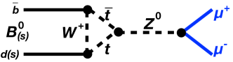
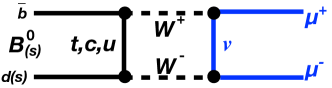
Figure 1: The decays $B^{0}_{s}\rightarrow\mu^{+}\mu^{-}$ and $B^{0}\rightarrow\mu^{+}\mu^{-}$ are mediated by (left) $Z$-penguin and (right) box diagrams. The latter is suppressed by $(m_{W}/m_{t})^{2}$ with respect to the former.

The heavy and light mass eigenstates of the $B^{0}_{s}$ meson, $|B_{s,L(H)}^{0}\rangle=p|B^{0}_{s}\rangle\pm q|\kern 1.79993pt\bar{\kern-1.79993ptB}{}^{0}_{s}\rangle$ (with $|p|^{2}+|q|^{2}=1$), have different lifetimes. In the absence of $C\kern-1.99997ptP$ violation, only the $C\kern-1.99997ptP$-odd heavy $B^{0}_{s}$ state, with a lifetime of $\tau_{B_{s,H}^{0}}=1.615\pm 0.009\mbox{\,ps}$ [8], can decay into the dimuon final state via the SM interactions. Because this fact is independent of the predicted numerical value of the branching fraction, it is of high interest to measure also the $B^{0}_{s}\rightarrow\mu^{+}\mu^{-}$ effective lifetime, defined [9] as the time expectation value of the untagged rate by

$$\tau_{\mu^{+}\mu^{-}}\equiv\frac{\int_{0}^{\infty}t\,[\Gamma(B^{0}_{s}(t)\rightarrow\mu^{+}\mu^{-})+\Gamma(\kern 1.79993pt\bar{\kern-1.79993ptB}{}^{0}_{s}(t)\rightarrow\mu^{+}\mu^{-})]\,dt}{\int_{0}^{\infty}[\Gamma(B^{0}_{s}(t)\rightarrow\mu^{+}\mu^{-})+\Gamma(\kern 1.79993pt\bar{\kern-1.79993ptB}{}^{0}_{s}(t)\rightarrow\mu^{+}\mu^{-})]\,dt},$$ (1)

where $t$ is the proper decay time of the $B^{0}_{s}$ meson. Experimentally, $\tau_{\mu^{+}\mu^{-}}$ is determined by fitting a single exponential function, corrected for experimental artifacts like efficiency and resolution, to the decay time distribution of $B^{0}_{s}\rightarrow\mu^{+}\mu^{-}$ decays.

In the SM the branching fractions for these decays have been calculated beyond leading order in quantum chromodynamics (QCD) since more than a quarter century (cf. Fig. 2 and references therein). Most recently, computations of three-loop QCD corrections [2], electroweak effects at next-to-leading order [3], and enhanced electromagnetic corrections [4, 5] have been completed. The (relative) errors are estimated to be smaller than 5% in the most recent calculation. By now, the theoretical error budget is dominated by external parametric uncertainties (either from CKM matrix element magnitudes or the $B$ meson decay constant, depending on the number of dynamical quark flavors in the lattice QCD calculations [10]).

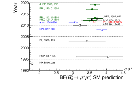
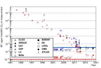
Figure 2: (left) Time evolution of the SM prediction. Note that the top quark was not yet discovered at the time of the first prediction beyond leading order and that many parameters were significantly off from today’s values. (right) The experimental results for the branching fraction ${\overline{\mathcal{B}}}(B^{0}_{s}\rightarrow\mu^{+}\mu^{-})$, shown with blue symbols for upper limits and black symbols for measurements, and upper limits for ${\mathcal{B}}(B^{0}\rightarrow\mu^{+}\mu^{-})$, shown in red symbols.

The experimental effort has been pursued both at $e^{+}$$e^{-}$ machines for $B^{0}\rightarrow\mu^{+}\mu^{-}$ and at hadron colliders for $B^{0}_{s}\rightarrow\mu^{+}\mu^{-}$ (and $B^{0}\rightarrow\mu^{+}\mu^{-}$). The impressive sensitivity progression in the past four decades is illustrated in Fig. 2 (right). At the Large Hadron Collider (LHC), the decay $B^{0}_{s}\rightarrow\mu^{+}\mu^{-}$ has been measured with at least four standard deviation ($\sigma$) significances by the ATLAS [11], CMS [12], and LHCb [13] collaborations. More recently, LHCb [14] and CMS [15] (with the result discussed here) each have reached more than $5\sigma$ individually. The $B^{0}_{s}\rightarrow\mu^{+}\mu^{-}$ effective lifetime has been measured first by the LHCb collaboration [14] and now by the CMS collaboration [15]. All confirmed results to date are in agreement with the SM predictions.

2 Experimental Strategy

The experimental approach starts with reconstructing dimuon candidates in a wide invariant mass region. The number of background candidates is reduced with advanced muon identification algorithms and multivariate analysis techniques in the selection. Finally, the number of signal decays is determined with an unbinned maximum likelihood fit to the mass distribution and other variables. Signal $B\rightarrow\mu^{+}\mu^{-}$ decays are characterized by two muons, with an invariant mass $m_{\mu\mu}$ around the $B^{0}$ or $B^{0}_{s}$ mass, originating from a common point in space where the $B$ meson decayed. The background has several components with characteristics that allow its reduction with respect to the signal:

• Combinatorial background from two semileptonic $B$ decays or from one semileptonic $B$ decay together with a hadron misidentified as a muon (fake muon). The two muons do not originate from the same point in space. This component is the limiting factor for the measurement of $B^{0}_{s}\rightarrow\mu^{+}\mu^{-}$.

• Rare decays of a single $B$ hadron, illustrated in Fig. 3 (left). They consist of decays with (1) two muons (e.g., $B^{0}\rightarrow\pi^{0}\mu^{+}\mu^{-}$, where the pion is not considered in the final state reconstruction), (2) one muon combined with a fake muon (e.g., $B^{0}_{s}\rightarrow K^{-}\mu^{+}\nu$), or (3) with two fake muons (e.g., $B^{0}_{s}\rightarrow K^{+}K^{-}$). These decays constitute a dangerous background affecting in particular $B^{0}\rightarrow\mu^{+}\mu^{-}$. In the first two cases, the mass distribution is leaking into the $B^{0}$ mass region, but the missing particle provides a handle to reduce this contribution. The last case constitutes a peaking background near the $B^{0}$ mass region. The wrong mass hypothesis, muon instead of kaon or pion, shifts the mass distribution from the $B^{0}_{s}$ mass to lower values.

In the discussion above, a fake muon is a hadron misidentified in the detector as a muon, either because of its decay-in-flight or punch-through (hits in the muon system associated to a charged track).

     

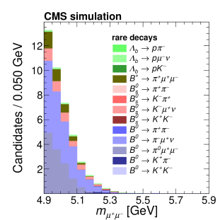
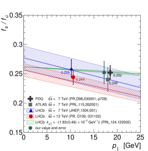
Figure 3: (left) Background invariant mass distribution from rare $B$ decays with 0, 1, or 2 fake muons (hadrons misidentified as muons). It can be deduced from the plot that these decays are much more dangerous for $B^{0}\rightarrow\mu^{+}\mu^{-}$ than for $B^{0}_{s}\rightarrow\mu^{+}\mu^{-}$ because of (1) their mass distribution covering the $B^{0}$ mass region ($m_{B^{0}}=5.280\mbox{\,Ge\kern-1.00006ptV}$ [8]) more strongly than the $B^{0}_{s}$ mass region ($m_{B^{0}_{s}}=5.367\mbox{\,Ge\kern-1.00006ptV}$ [8]) and (2) the suppressed rate of $B^{0}\rightarrow\mu^{+}\mu^{-}$ compared to $B^{0}_{s}\rightarrow\mu^{+}\mu^{-}$. (right) Illustration of measurements of $f_{s}/f_{u}$, the ratio of the $B^{0}_{s}$ and $B^{+}$ fragmentation probabilities for different mean $B$ meson transverse momentum $p_{\perp}$ and at different center-of-mass energies $\sqrt{s}$. The bands indicate the parametrizations of the LHCb experiment. The value adopted by CMS corresponds to the PDG [8] value, with an ad-hoc enlargement of the error (see text for more details). It is interesting to note that the most significant slope determination, shown in green, results in the smallest slope.

The branching fraction ${\mathcal{B}}(B^{0}_{s}\rightarrow\mu^{+}\mu^{-})$ is determined relative to a normalization sample with a well-known branching fraction. Starting from Ref. Abazov:2004dj, the decay $B^{+}\rightarrow{J\mskip-3.0mu/\mskip-2.0mu\psi\mskip 2.0mu}K^{+}$, with ${J\mskip-3.0mu/\mskip-2.0mu\psi\mskip 2.0mu}\rightarrow\mu^{+}\mu^{-}$, has been used as normalization schematically as follows:

$${\overline{\mathcal{B}}}(B^{0}_{s}\rightarrow\mu^{+}\mu^{-})=\frac{N_{B^{0}_{s}}}{N_{B^{+}}}\,\frac{f_{u}}{f_{s}}\,\frac{\varepsilon^{\text{tot}}_{B^{+}}}{\varepsilon^{\text{tot}}_{B^{0}_{s}}}\,{\mathcal{B}}(B^{+}\rightarrow{J\mskip-3.0mu/\mskip-2.0mu\psi\mskip 2.0mu}K^{+})\,{\mathcal{B}}({J\mskip-3.0mu/\mskip-2.0mu\psi\mskip 2.0mu}\rightarrow\mu^{+}\mu^{-}),$$ (2)

where $N_{B^{0}_{s}}(N_{B^{+}})$ is the number of signal $B^{0}_{s}\rightarrow\mu^{+}\mu^{-}$ ($B^{+}\rightarrow{J\mskip-3.0mu/\mskip-2.0mu\psi\mskip 2.0mu}K^{+}$) decays, $\varepsilon^{\text{tot}}_{B^{0}_{s}}$ ($\varepsilon^{\text{tot}}_{B^{+}}$) is the total signal ($B^{+}$) efficiency, ${\mathcal{B}}(B^{+}\rightarrow{J\mskip-3.0mu/\mskip-2.0mu\psi\mskip 2.0mu}K^{+})=(1.01\pm 0.03)\times 10^{-3}$ and ${\mathcal{B}}({J\mskip-3.0mu/\mskip-2.0mu\psi\mskip 2.0mu}\rightarrow\mu^{+}\mu^{-})=(5.96\pm 0.03)\times 10^{-2}$ [8], and $f_{u}/f_{s}$ is the ratio of the $B^{+}$ and $B^{0}_{s}$ fragmentation functions. A similar approach is used for ${\mathcal{B}}(B^{0}\rightarrow\mu^{+}\mu^{-})$, using $f_{d}/f_{u}=1$ [8].

In addition to serving as a ‘normalization sample’, the $B^{+}\rightarrow{J\mskip-3.0mu/\mskip-2.0mu\psi\mskip 2.0mu}K^{+}$ candidates also constitute a large sample of $B^{+}$ mesons where the Monte Carlo (MC) simulation can be validated against data. To compare $B^{0}_{s}$ mesons in data and MC simulation, a ‘control sample’ of $B^{0}_{s}\rightarrow{J\mskip-3.0mu/\mskip-2.0mu\psi\mskip 2.0mu}\phi$ (with ${J\mskip-3.0mu/\mskip-2.0mu\psi\mskip 2.0mu}\rightarrow\mu^{+}\mu^{-}$ and $\phi\rightarrow K^{+}K^{-}$) candidates is used. Because the analysis relies on MC simulation for the efficiency determination, the validation of the MC simulation is essential. Furthermore, these $B\rightarrow{J\mskip-3.0mu/\mskip-2.0mu\psi\mskip 2.0mu}X$ samples can be used to study differences between data and MC simulation regarding $b$ quark production processes (e.g., by combining such decays with another muon from a semileptonic $\kern 1.79993pt\bar{\kern-1.79993ptB}{}$ decay) and to study in detail the $b$ quark hadronization into $B^{0}_{s}$ or $B^{+}$ mesons.

The usage of $B^{+}\rightarrow{J\mskip-3.0mu/\mskip-2.0mu\psi\mskip 2.0mu}K^{+}$ as a normalization sample is motivated by the minimal difference in the final state with respect to the signal decay (one additional charged particle). This leads to a substantial reduction of the systematic uncertainties. However, it implies a direct dependence of ${\overline{\mathcal{B}}}(B^{0}_{s}\rightarrow\mu^{+}\mu^{-})$ on $f_{s}/f_{u}$ [though not for the effective $B^{0}_{s}\rightarrow\mu^{+}\mu^{-}$ lifetime or ${\mathcal{B}}(B^{0}\rightarrow\mu^{+}\mu^{-})$]. In Fig. 3 (right) the experimental situation of $f_{s}/f_{u}$ measurements and combinations is illustrated. The LHCb collaboration [17] obtains a significant slope vs. the transverse momentum ($p_{\perp}$) of the $B$ meson, while the ATLAS collaboration [18] and the CMS collaboration (internal study performed for the result discussed here) see no such effect. Nevertheless the CMS experiment decided to account for a hypothetical $p_{\perp}$ dependence and possible center-of-mass energy ($\sqrt{s}$) dependence by adding an ad-hoc error to $f_{s}/f_{u}$. An uncertainty of 0.008 is derived from the difference between the value of $f_{s}/f_{u}$ in Ref. pdg2018, obtained at $\sqrt{s}=7\mbox{\,Te\kern-1.00006ptV}$, and that in Ref. Aaij:2019pqz, obtained at $\sqrt{s}=13\mbox{\,Te\kern-1.00006ptV}$. In addition, with the parametrization of the $p_{\perp}$ dependence in Ref. Aaij:2019pqz, a difference of 0.013 is determined between the $f_{s}/f_{u}$ values at the average $p_{\perp}$ of Ref. Aaij:2019pqz and the average $p_{\perp}$ of the $B^{0}_{s}\rightarrow\mu^{+}\mu^{-}$ candidates in this analysis. Ref. Aaij:2019eej would imply a much smaller $p_{\perp}$ dependence, but was published too late to be included. In summary, the CMS experiment uses $f_{s}/f_{u}=0.252\pm 0.012(\text{exp})\pm 0.015(\text{CMS})$ where the first error is from the PDG [8] and the second error is the ad-hoc error of CMS.

In the future, a normalization to other decay modes may provide a less contentious solution. While ${\mathcal{B}}(B^{0}_{s}\rightarrow{J\mskip-3.0mu/\mskip-2.0mu\psi\mskip 2.0mu}\phi)$ normally has a dependence on $f_{s}/f_{d}$ (or $f_{s}/f_{u}$) when determined at hadron colliders, results obtained at $e^{+}$$e^{-}$ machines at the $\mathchar 28935\relax{(5S)}$ provide additional input and may lead to a smaller overall error.

To avoid a possible bias, the analyses searching for and measuring the $B\rightarrow\mu^{+}\mu^{-}$ decays have been pursued as ‘blind’ analyses since a long time. This implies that a signal region, often defined in terms of the invariant mass, is hidden during the development and optimization of the analysis methodology. To take full advantage of analysis improvements (e.g., improved muon identification, re-processed data with better tracking resolutions, etc.) it is advantageous to re-analyze the old, previously published, datasets. This implies a ‘re-blinding’ of the data, which is, however, not a problem because the improvements normally change the set of candidates noticeably. An alternative would be to combine new results only statistically with the old results, albeit at a loss of sensitivity. In this analysis, the first approach is used and the dimuon mass range $5.2<m_{\mu\mu}<5.45\mbox{\,Ge\kern-1.00006ptV}$ was kept (re-)blinded until the entire selection and fitting procedure was finalized.

3 Detector and Data

The data for this analysis was collected by the CMS experiment [20] in LHC Run 1 (25$\mbox{\,fb}^{-1}$) and in 2016 (36$\mbox{\,fb}^{-1}$), as summarized in Table 3. The CMS experiment is very well suited for $B\rightarrow\mu^{+}\mu^{-}$ measurements because its silicon tracker, composed of a pixel detector with 66 million pixels of $100\,\mu\mbox{m}\times 150\,\mu\mbox{m}$ and a micro-strip detector with 10 million strips with pitches between $80$ and $180\,\mu\mbox{m}$, provides outstanding three-dimensional (3D) vertexing and tracking capabilities in a very homogeneous solenoidal magnetic field of $3.8\mbox{\,T}$. The tracker is divided into barrel and endcap parts. In Run 2, the micro-strip detector was subject to operational instabilities and the data are therefore divided into two separate data-taking periods, 2016A and 2016B, of 16$\mbox{\,fb}^{-1}$and 20$\mbox{\,fb}^{-1}$, respectively. The systematic error of the tracking efficiency is estimated [21, 22] to be 4% (2.3%) in Run 1 (2016).

Summary of the data, together with center-of-mass energy $\sqrt{s}$, the integrated luminosity ${\mathcal{L}}$, the pileup quantified as the average number of $pp$ collision vertices reconstructed as primary vertices $\langle N_{\text{PV}}\rangle$, and the channel definition based on the pseudorapidity of the most-forward muon $|\eta_{\mu}^{\text{f}}|$. Note that in Run 2 (2016A and 2016B) the region $|\eta_{\mu}^{\text{f}}|>1.4$ (the forward channel of Run 1) is no longer present because of trigger rate constraints. Data-taking $\sqrt{s}$ ${\mathcal{L}}$ Pileup Channels period [ TeV] [$\mbox{\,fb}^{-1}$] $\langle N_{\text{PV}}\rangle$ central forward 2011 7 5 8 $0<|\eta_{\mu}^{\text{f}}|<1.4$ $1.4<|\eta_{\mu}^{\text{f}}|<2.1$ 2012 8 20 15 $0<|\eta_{\mu}^{\text{f}}|<1.4$ $1.4<|\eta_{\mu}^{\text{f}}|<2.1$ 2016A 13 16 18 $0<|\eta_{\mu}^{\text{f}}|<0.7$ $0.7<|\eta_{\mu}^{\text{f}}|<1.4$ 2016B 13 20 18 $0<|\eta_{\mu}^{\text{f}}|<0.7$ $0.7<|\eta_{\mu}^{\text{f}}|<1.4$

Muons are detected in four muon stations, using three complementary detector types, interspersed among the steel flux-return plates. Standalone muons are formed from hits in the muon stations and combined with silicon tracker tracks to form so-called global muons [23, 24]. A dedicated boosted decision tree (BDT) was trained separately for Run 1 and Run 2 data to obtain the best possible hadron-to-muon misidentification probability. The starting point for this BDT are global muons. The variables used in the BDT are based on measurements from the (1) silicon tracker, (2) the muon system, and (3) the combined global muon reconstruction. This new muon BDT achieves an average muon misidentification probability of $6\times 10^{-4}$ and $10^{-3}$ for pions and kaons, respectively, with a muon identification efficiency of about 75%. Compared to the previous analysis [12], the muon BDT is operated at a significantly lower muon misidentification rate and roughly the same muon identification efficiency. The muon BDT is extensively validated with kinematically identified samples of muons, pions, kaons, and protons (from the decays ${J\mskip-3.0mu/\mskip-2.0mu\psi\mskip 2.0mu}\rightarrow\mu^{+}\mu^{-}$, $K^{0}_{\scriptscriptstyle S}\rightarrow\pi^{+}\pi^{-}$, $\phi\rightarrow K^{+}K^{-}$, and $\mathchar 28931\relax\rightarrow p\pi^{-}$, respectively) in data and MC simulation. All distributions of variables used in the muon BDT, the BDT discriminator distributions, and the absolute muon misidentification probability are found to be consistent between data and simulation. The systematic error for the muon efficiency is determined from the difference of the efficiency ratio of the muon BDT discriminator requirement for $B^{+}\rightarrow{J\mskip-3.0mu/\mskip-2.0mu\psi\mskip 2.0mu}K^{+}$ and $B^{0}_{s}\rightarrow{J\mskip-3.0mu/\mskip-2.0mu\psi\mskip 2.0mu}\phi$ between data and simulation, which agrees to better than 3%. The systematic error on the muon misidentification is derived from a direct comparison of the absolute muon misidentification probability in data and simulation (10% relative uncertainty for pions and kaons). For protons, the very small sample size of $\mathchar 28931\relax\rightarrow p\pi^{-}$, with a misidentified proton, does not allow this approach and the error of the average muon misidentification probability, in data and simulation, is used instead (60% relative uncertainty).

The trigger [25] of the CMS experiment has two stages: the first stage is based on custom hardware processors and selects two muons with either no or minimal $p_{\perp}^{\mu}$ threshold (because of the strong magnetic field, there is an implicit $p_{\perp}^{\mu}$ threshold of about $3.5\mbox{\,Ge\kern-1.00006ptV}$ in the central region). The second stage, the high-level trigger (HLT) consists of a processor farm running the full event reconstruction software with reduced sets of calibration constants. The normalization sample is triggered with a setup that is very similar to the signal setup with the exception that the two muons must be consistent with originating from a ${J\mskip-3.0mu/\mskip-2.0mu\psi\mskip 2.0mu}$ meson from a $B$ decay (‘displaced ${J\mskip-3.0mu/\mskip-2.0mu\psi\mskip 2.0mu}$’). The signal (normalization) trigger efficiency varies over the data-taking periods from 65–75% (50–75%). The systematic uncertainty on the ratio of the trigger efficiency is estimated to be 3%.

The tracking detectors of the CMS experiment induce a strong pseudorapidity ($\eta$) dependence of the mass resolution. Therefore the analysis sensitivity benefits from subdividing the data into ‘channels’, according to the $\eta$ of the most forward muon. Because of trigger changes over the years, the boundary between the ‘central’ and ‘forward’ channels is different between Run 1 and Run 2. In total, there are eight channels in the analysis (central and forward in four data-taking periods) as summarized in Table 3.

At the instantaneous luminosity of the LHC, multiple $pp$ interactions (pileup) occur in each bunch crossing. Tracks from other $pp$ interaction vertices (primary vertices or PVs) increase the combinatorial background and complicate the determination of key variables in the selection, as discussed below. Table 3 lists the average number of PVs reconstructed in the different data-taking periods.

4 Candidate Selection

The $B\rightarrow\mu^{+}\mu^{-}$ candidate reconstruction starts with two global muons with $p_{\perp}^{\mu}>4\mbox{\,Ge\kern-1.00006ptV}$ and a small distance of closest approach $d_{\text{ca}}<0.8\mbox{\,cm}$ between their trajectories. The two muons are constrained to originate from a common point (secondary vertex or SV) and to have an invariant mass $4.9<m_{\mu\mu}<5.9\mbox{\,Ge\kern-1.00006ptV}$, after refitting their momenta to include the SV as an additional hit. For each reconstructed $B$ candidate one specific PV is chosen as the $B$-meson origin (denoted below as $B$-PV), based on the longitudinal impact parameter $\ell_{z}$ along the beam axis of the extrapolated $B$-meson trajectory. The PVs are refitted by excluding tracks from the $B$ candidate. The variables involved in the selection are sketched in Fig. 4 (left) for a signal event. The $B\rightarrow\mu^{+}\mu^{-}$ selection exploits the differences between signal and background. Signal $B\rightarrow\mu^{+}\mu^{-}$ decays are characterized by a SV with a good fit $\chi^{2}/{\text{dof}}$, separated from the $B$-PV by a large flight length $\ell_{3D}$ and significance $\ell_{3D}/\sigma(\ell_{3D})$, where $\sigma(\ell_{3D})$ is the error of $\ell_{3D}$. The $B$-meson proper decay time is measured as $t=m_{\mu\mu}\ell_{3D}/p^{\mu^{+}\mu^{-}}$ in 3D space. The $B$-meson momentum is well aligned with the flight direction (the direction from the $B$-PV to the SV), implying a small opening angle $\alpha_{3\text{D}}$ and a small $B$ impact parameter $\delta_{3D}$ and significance $\delta_{3D}/\sigma(\delta_{3D})$.

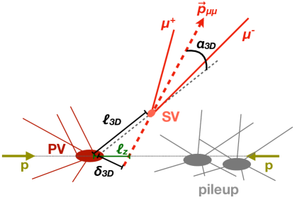
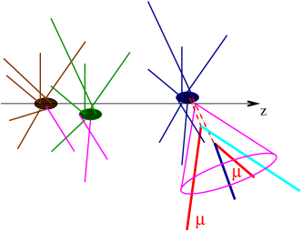
Figure 4: (left) Sketch of a signal decay with the variables involved (see text for a description). (right) Sketch of a background decay showing aspects of the candidate isolation. Tracks from pileup PVs that would fall within the isolation cone (shown in pink) are excluded from the isolation calculation by requiring that all tracks considered are associated with the $B$-PV or are close to the SV (see text for more details).

For a signal decay, the two muons are the only final-state particles of the $B$ meson decay, and therefore the $B$ meson and the muons are isolated, i.e., not many other charged tracks are nearby. This isolation is quantified by two sets of variables. The first set determines a macroscopic isolation $I$ using

$$I=\frac{p_{\perp}^{B}}{p_{\perp}^{B}+\sum_{\mathrm{trk}}p_{\perp}^{\mathrm{trk}}},$$ (3)

where the sum includes all tracks, not part of the $B$ candidate, inside a cone with radius $\Delta R=\sqrt{(\Delta\eta)^{2}+(\Delta\varphi)^{2}}<0.7$, where $\Delta\eta$ $(\Delta\varphi)$ is the difference between the track and the $B$ candidate $\eta$ (azimuthal angle $\varphi$). Because of tracks from other PVs not related to the $B$-PV, it is essential to only use tracks that are either associated to the $B$-PV or are close to the SV. Without these requirements, the tracks from other pileup PVs would bias $I$, as indicated in Fig. 4 (right) for a background event. The tracks in the sum must fulfill $\mbox{$p_{\perp}$}>0.9\mbox{\,Ge\kern-1.00006ptV}$ and have $d_{\text{ca}}^{\text{SV}}<0.05\mbox{\,cm}$ with respect to the SV. These requirements were optimized with $B\rightarrow{J\mskip-3.0mu/\mskip-2.0mu\psi\mskip 2.0mu}X$ decays for strongest background rejection and best agreement between data and simulation. Similar isolation variables, $I_{\mu_{1}}$ and $I_{\mu_{2}}$, are determined for each of the two muons, although with different track requirements in the sum, $\mbox{$p_{\perp}$}>0.5\mbox{\,Ge\kern-1.00006ptV}$ and $d_{\text{ca}}^{\text{SV}}<0.1\mbox{\,cm}$, and a smaller cone radius of $\Delta R=0.5$.

The second set of isolation variables is based on microscopic observables determined with tracks of $\mbox{$p_{\perp}$}>0.5\mbox{\,Ge\kern-1.00006ptV}$ that are not part of the $B$ candidate and are not associated to any non-$B$-PV (i.e., if they are associated to a PV it must be the $B$-PV): the minimum distance of closest approach, $d^{\text{0}}_{\text{ca}}$, of any qualifying track to the SV and $N_{\text{trk}}^{\text{close}}$, the number of tracks with $d_{\text{ca}}^{\text{SV}}<0.03\mbox{\,cm}$ to the SV.

Many of these variables are correlated with each other. For instance, the flight length and its significance are correlated with $N_{\text{trk}}^{\text{close}}$, and the isolation variables $I$, $I_{\mu_{1}}$, and $I_{\mu_{2}}$are correlated with each other. A robust approach in such a situation is to train a multivariate analysis technique [26] in the form of a BDT. This selection BDT was trained on $B^{0}_{s}\rightarrow\mu^{+}\mu^{-}$ and $B^{0}\rightarrow\mu^{+}\mu^{-}$ signal decays from MC simulation and combinatorial background from the data sideband $5.45<m_{\mu\mu}<5.9\mbox{\,Ge\kern-1.00006ptV}$. Since data events are used in the training, the MC and data samples were randomly split into three subsets to ensure that the training and validation of a BDT are performed on subsets completely independent of its application. This procedure implies that three BDTs are required for the analysis of each channel. A preselection removes candidates with extreme outlier values in the variables and requires the SV to be well separated from the $B$-PV, $\ell_{3D}/\sigma(\ell_{3D})>4$. With the subdivision of the data into three subsets per channel, the number of events available for training is somewhat limited after the preselection (at least 6000 candidates in any subset). For the per-channel optimization of the BDT configuration, a set of core variables [$\ell_{3D}/\sigma(\ell_{3D})$, $\alpha_{3\text{D}}$, $\delta_{3D}/\sigma(\delta_{3D})$, $d^{\text{0}}_{\text{ca}}$, $\chi^{2}/{\text{dof}}$, $N_{\text{trk}}^{\text{close}}$, $I$, $I_{\mu_{1}}$, $I_{\mu_{2}}$] is iteratively combined with a subset of other $B$-candidate variables [$d_{\text{ca}}$, $\delta_{3D}$, $\ell_{3D}$, $\ell_{xy}/\sigma(\ell_{xy})$, $p_{\perp}^{B}$, $\eta_{B}$]. The best BDT configurations are chosen based on (1) the maximum of $S/\sqrt{S+B}$, where $S$ ($B$) is the expected $B^{0}_{s}\rightarrow\mu^{+}\mu^{-}$ signal (combinatorial background, extrapolated from the sideband) yield in the mass region $5.3<m_{\mu\mu}\ <5.45\mbox{\,Ge\kern-1.00006ptV}$ and (2) the visual assessment of the agreement between data and MC simulation using large samples of exclusive $B\rightarrow{J\mskip-3.0mu/\mskip-2.0mu\psi\mskip 2.0mu}X$ candidates.

The decays $B^{+}\rightarrow{J\mskip-3.0mu/\mskip-2.0mu\psi\mskip 2.0mu}K^{+}$ and $B^{0}_{s}\rightarrow{J\mskip-3.0mu/\mskip-2.0mu\psi\mskip 2.0mu}\phi$, both with ${J\mskip-3.0mu/\mskip-2.0mu\psi\mskip 2.0mu}\rightarrow\mu^{+}\mu^{-}$, allow the validation of the selection BDT and serve as normalization and control samples, respectively. Their reconstruction starts with two oppositely charged muons with $p_{\perp}^{\mu}>4\mbox{\,Ge\kern-1.00006ptV}$, $p_{\perp}^{\mu^{+}\mu^{-}}>7\mbox{\,Ge\kern-1.00006ptV}$, and $2.9<m_{\mu\mu}<3.2\mbox{\,Ge\kern-1.00006ptV}$. They are combined with one or two tracks, respectively, assumed to be kaons and with $\mbox{$p_{\perp}$}>0.6\mbox{\,Ge\kern-1.00006ptV}$. To reduce combinatorial background, the maximum distance of closest approach between any pair of tracks is required to fulfill $d_{\text{ca}}^{\text{max}}<0.08\mbox{\,cm}$. For $B^{0}_{s}\rightarrow{J\mskip-3.0mu/\mskip-2.0mu\psi\mskip 2.0mu}\phi$, the two tracks must fulfill $1.01<m_{K^{+}K^{-}}<1.03\mbox{\,Ge\kern-1.00006ptV}$. To allow the selection of the $B\rightarrow{J\mskip-3.0mu/\mskip-2.0mu\psi\mskip 2.0mu}X$ candidates with the same selection BDT as for the signal $B\rightarrow\mu^{+}\mu^{-}$ decays, their variable distributions should mirror the corresponding ones from signal decays. This implies that the SV $\chi^{2}/{\text{dof}}$ is not based on the full SV fit with three or four tracks, but only on the dimuon vertex fit. In addition, for all isolation variables, the kaon track(s) are not part of the track sums of Eq. 3. Example mass distributions, together with fits to the data using signal (double Gaussian functions with a common mean) and background components, are shown in Fig. 5. The background components for $B^{+}\rightarrow{J\mskip-3.0mu/\mskip-2.0mu\psi\mskip 2.0mu}K^{+}$ contain an exponential function for the combinatorial background, an error function for partially reconstructed $B\rightarrow{J\mskip-3.0mu/\mskip-2.0mu\psi\mskip 2.0mu}K^{+}X$ decays, and a MC simulation based shape for the peaking background from $B^{+}\rightarrow{J\mskip-3.0mu/\mskip-2.0mu\psi\mskip 2.0mu}\pi^{+}$ (fixed to 4%[8] of the total signal yield). For $B^{0}_{s}\rightarrow{J\mskip-3.0mu/\mskip-2.0mu\psi\mskip 2.0mu}\phi$ the background is parametrized by an exponential function for the combinatorial component and a MC simulation based shape for the peaking background from $B^{0}\rightarrow{J\mskip-3.0mu/\mskip-2.0mu\psi\mskip 2.0mu}K^{*0}$, with $K^{*0}\rightarrow K^{+}\pi^{-}$ (where the pion is treated as a kaon). The total $B^{+}\rightarrow{J\mskip-3.0mu/\mskip-2.0mu\psi\mskip 2.0mu}K^{+}$ normalization yield used for the determination of ${\mathcal{B}}(B^{0}_{s}\rightarrow\mu^{+}\mu^{-})$ is $N_{B^{+}}=(1.43\pm 0.06)\times 10^{6}$, where the error is dominated by the systematic component of (relative) 4%, obtained from the yield comparison between fits without and with ${J\mskip-3.0mu/\mskip-2.0mu\psi\mskip 2.0mu}$-mass constraints.

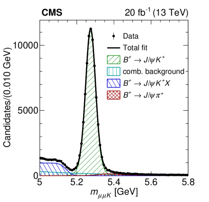
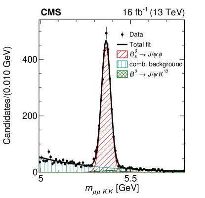
Figure 5: Invariant mass distribution for (left) the normalization sample $B^{+}\rightarrow{J\mskip-3.0mu/\mskip-2.0mu\psi\mskip 2.0mu}K^{+}$ and (right) the control sample $B^{0}_{s}\rightarrow{J\mskip-3.0mu/\mskip-2.0mu\psi\mskip 2.0mu}\phi$. The data are shown by solid black circles, the result of the fit is overlaid with the thick solid black line, and the different components are shown with hatched regions.

Background-subtracted variable distributions in data are compared to the corresponding distributions in the MC simulation. In Fig. 6 the distributions for the $p_{\perp}$ of the subleading muon (the muon with the lower $p_{\perp}$) and the $\ell_{3D}/\sigma(\ell_{3D})$ of the $B^{+}$ meson are shown as examples. The MC simulation provides a reasonable description of the data; the remaining discrepancies are fully accounted for in the systematic uncertainty. The pileup dependence of the HLT tracking in Run 2 affects the normalization sample stronger than the signal sample because of the displacement requirement in the $B^{+}\rightarrow{J\mskip-3.0mu/\mskip-2.0mu\psi\mskip 2.0mu}K^{+}$ HLT path. This is corrected for with an offline reweighting depending on the number of reconstructed PV and $\ell_{xy}/\sigma(\ell_{xy})$. The remaining systematic error from this corrections is estimated to be 6% for 2016A and 5% for 2016B for the branching fraction measurement. For the $B^{0}_{s}\rightarrow\mu^{+}\mu^{-}$ effective lifetime measurement, a systematic error of $0.07\mbox{\,ps}$ is estimated. This is the second-largest systematic uncertainty for both results.

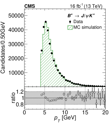
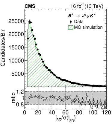
Figure 6: Comparison of the measured and simulated distributions of (left) the subleading muon $p_{\perp}$ and (right) the flight length significance $\ell_{3D}/\sigma(\ell_{3D})$ for $B^{+}\rightarrow{J\mskip-3.0mu/\mskip-2.0mu\psi\mskip 2.0mu}K^{+}$ decays in data and MC simulation. Background-subtracted data are shown by solid black circles, the MC simulation by hatched histograms. In the lower panels the ratio between data and MC simulation is shown. The band at $\pm 20\%$ is just to guide the eye.

In Fig. 7 the BDT discriminator response is shown for dimuon candidates, illustrating the background rejection, and for $B^{+}\rightarrow{J\mskip-3.0mu/\mskip-2.0mu\psi\mskip 2.0mu}K^{+}$ candidates, illustrating the agreement between data and MC simulation. The systematic error of the selection efficiency is estimated from the double ratio

$$D=\frac{\left[\frac{\varepsilon(B^{+}\rightarrow{J\mskip-3.0mu/\mskip-2.0mu\psi\mskip 2.0mu}K^{+})}{\varepsilon(B^{0}_{s}\rightarrow{J\mskip-3.0mu/\mskip-2.0mu\psi\mskip 2.0mu}\phi)}\right]_{\text{data}}}{\left[\frac{\varepsilon(B^{+}\rightarrow{J\mskip-3.0mu/\mskip-2.0mu\psi\mskip 2.0mu}K^{+})}{\varepsilon(B^{0}_{s}\rightarrow{J\mskip-3.0mu/\mskip-2.0mu\psi\mskip 2.0mu}\phi)}\right]_{\text{MC}}},$$ (4)

where the control sample $B^{0}_{s}\rightarrow{J\mskip-3.0mu/\mskip-2.0mu\psi\mskip 2.0mu}\phi$ is used as a placeholder for the signal sample. Depending on the channel, this systematic error varies between 5% and 10%. It constitutes the largest contribution to the overall systematic error for the branching fraction. The selection efficiency depends on the unknown true effective lifetime because of the displacement and isolation criteria. This uncertainty of 1–3%, depending on data-taking period and analysis channel, is estimated with $\Delta\equiv[\varepsilon_{\text{tot}}(\tau_{B_{s,H}^{0}})-\varepsilon_{\text{tot}}(\tau_{B_{s,L}^{0}})]/\sqrt{12}$ using simulated samples with different effective lifetimes.

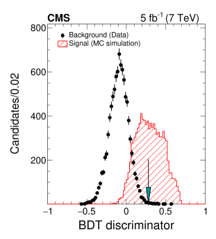
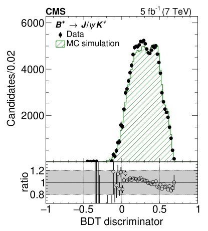
Figure 7: Comparison of the BDT discriminator response for (left) dimuons in data (background from the invariant mass sideband $5.45<m_{\mu\mu}<5.9\mbox{\,Ge\kern-1.00006ptV}$) and MC simulation ($B^{0}_{s}\rightarrow\mu^{+}\mu^{-}$ signal) and (right) $B^{+}\rightarrow{J\mskip-3.0mu/\mskip-2.0mu\psi\mskip 2.0mu}K^{+}$ candidates in data and MC simulation. The left plot illustrates the rejection power of the BDT against (combinatorial) background, the right plot shows the level of agreement between data and MC simulation, an ingredient in the determination of the systematic error of the analysis efficiency. The arrow in the left plot indicates the category boundary of the BDT discriminator range used in the ${\mathcal{B}}(B^{0}_{s}\rightarrow\mu^{+}\mu^{-})$ result determination (cf. Table 5 below).

The mixture of $b\overline{b}$ quark production processes in the MC simulation is not necessarily the same as in data. At leading order three processes contribute to heavy quark production in $pp$ collisions: gluon splitting, gluon-gluon fusion, and flavor excitation. The $b$ quarks from gluon splitting are closer together in phase space than for the other two processes, where the two $b$ quarks tend to be back-to-back in the transverse plane. Therefore a $B^{0}_{s}\rightarrow\mu^{+}\mu^{-}$ decay from a $B^{0}_{s}$ meson produced in gluon splitting will be, on average, less isolated than from a $B^{0}_{s}$ meson from gluon-gluon fusion. Therefore a mismatch of the production process mixture in data and simulation will imply a systematic uncertainty on the selection efficiency. The mixture of production processes is studied by combining a $B^{+}\rightarrow{J\mskip-3.0mu/\mskip-2.0mu\psi\mskip 2.0mu}K^{+}$ ($B^{0}_{s}\rightarrow{J\mskip-3.0mu/\mskip-2.0mu\psi\mskip 2.0mu}\phi$) candidate with another muon $\mu_{3}$ (assumed to originate from the semileptonic decay of the other $b$ hadron in the event) and studying the $\Delta R(B,\mu_{3})$ distribution. Fitting templates from MC simulation for gluon-splitting and the sum of gluon-gluon fusion plus flavor excitation to the data allows an estimate of the systematic uncertainty for the efficiency ratio at the 3% level.

As a cross check, the effective branching fraction ${\mathcal{B}}(B^{0}_{s}\rightarrow{J\mskip-3.0mu/\mskip-2.0mu\psi\mskip 2.0mu}\phi)$ was determined with an approach equivalent to Eq. 2, where the number of $B^{0}_{s}\rightarrow{J\mskip-3.0mu/\mskip-2.0mu\psi\mskip 2.0mu}\phi$ decays is used for $N_{B^{0}_{s}}$, for all channels in all data-taking periods. The standard deviation of these eight measurements is 4%, smaller than the combination of the systematic uncertainties due to analysis efficiency, tracking efficiency (the decay $B^{0}_{s}\rightarrow{J\mskip-3.0mu/\mskip-2.0mu\psi\mskip 2.0mu}\phi$ has one additional kaon track compared to $B^{+}\rightarrow{J\mskip-3.0mu/\mskip-2.0mu\psi\mskip 2.0mu}K^{+}$), hadronization uncertainties ($B^{0}_{s}$ vs. $B^{+}$), and yield determinations. Therefore we conclude that the systematic error is not underestimated.

Efficiency-corrected yield ratios for $B^{+}\rightarrow{J\mskip-3.0mu/\mskip-2.0mu\psi\mskip 2.0mu}K^{+}$, $B^{0}_{s}\rightarrow{J\mskip-3.0mu/\mskip-2.0mu\psi\mskip 2.0mu}\phi$, and $B^{0}\rightarrow{J\mskip-3.0mu/\mskip-2.0mu\psi\mskip 2.0mu}K^{*0}$ (with $K^{*0}\rightarrow K^{+}\pi^{-}$) decays are studied in the range $10<p_{\perp}^{B}<100\mbox{\,Ge\kern-1.00006ptV}$ and $0<|\eta_{B}|<2.2$ to estimate a possible dependence on these kinematic variables. No significant slope is observed vs. $p_{\perp}^{B}$ or $\eta_{B}$ for $f_{s}/f_{u}$, $f_{s}/f_{d}$, or $f_{d}/f_{u}$ (as a control measurement).

5 Results

For the determination of the results, the per-channel event samples are further subdivided into mutually exclusive categories of different signal-to-background ratios by introducing high- and low-BDT categories in the BDT discriminator distributions. This is illustrated in Fig. 7 (left), where the arrow shows the boundary between these categories. This categorization was optimized separately for the branching fraction measurement and the effective lifetime measurements. Table 5 provides the category boundaries. They vary over the channels because the BDT configuration has been optimized independently for each channel and results in different BDT discriminator distributions.

BDT discriminator category boundaries for the branching fraction measurement (left part) and the effective lifetime measurements (right part). These boundaries are illustrated in Fig. 7 (left). In the 2011 data-taking period, there is no low-BDT category because of the limited number of events. branching fraction measurement effective lifetime measurement central forward central forward 2011 {0.28, 1} {0.21, 1} {0.22, 1} {0.19, 1} 2012 {0.27, 0.35, 1} {0.23, 0.32, 1} {0.32, 1} {0.32, 1} 2016A {0.19, 0.30, 1} {0.19, 0.30, 1} {0.22, 1} {0.30, 1} 2016B {0.18, 0.31, 1} {0.23, 0.38, 1} {0.22, 1} {0.29, 1}

The branching fractions ${\overline{\mathcal{B}}}(B^{0}_{s}\rightarrow\mu^{+}\mu^{-})$ and ${\mathcal{B}}(B^{0}\rightarrow\mu^{+}\mu^{-})$ are determined with a 3D unbinned extended maximum likelihood fit to the dimuon invariant mass distribution, the relative mass resolution, and the binary distribution for the dimuon pairing configuration ${\cal C}$ (${\cal C}=\pm 1$ for the two muons bending towards or away from each other, respectively). While the first two variables have been used already in the past [12], the last variable was added as a protection against a possible underestimation of the $B\rightarrow h^{+}h^{-}$ background (critical for the $B^{0}\rightarrow\mu^{+}\mu^{-}$ measurement). Such an underestimate is possible because the $B\rightarrow h^{+}h^{-}$ contribution is determined under the assumption that the dimuon fake rate is the product of the single muon fake rates. While there is no evidence for such an underestimation for ${\cal C}=-1$ with the muons bending away from each other, the situation is less clear for ${\cal C}=+1$ where the muon tracks can be close together in the muon system. Since the effect is different for the two configurations, the ${\cal C}$ distribution is introduced. Its shape is taken from MC simulation for the signal and all background components. In the fit, a scale factor is used to correct the expected background component yields for the case ${\cal C}=+1$. A second, independent approach to control such an underestimate is to strongly reduce the muon misidentification probability (in this analysis, the misidentification probability was reduced by about 50% compared to the previous analysis [12]).

The signal probability density functions (PDFs) are based on a Crystal Ball function [27] for the invariant mass and a nonparametric kernel estimator [28] based on Gaussian kernels for the relative mass resolution. Table 5 provides a summary of all PDFs, for the branching fraction fit and the effective lifetime fit. The width of the Crystal Ball function is a conditional parameter with linear dependence on the dimuon mass resolution. All parameters, except for the signal yields, are fixed to values obtained from the MC simulation. Differences in the mass scale, studied with ${J\mskip-3.0mu/\mskip-2.0mu\psi\mskip 2.0mu}\rightarrow\mu^{+}\mu^{-}$ and $\mathchar 28935\relax{(1S)}\rightarrow\mu^{+}\mu^{-}$ and interpolated to $m_{B^{0}_{s}}$, are taken into account by shifting the MC mass distributions. The difference in the mass resolution between data and MC simulation has an effect of less than $0.2\%$ on the final results and is neglected.

Summary of the PDFs used for signal and background components in the unbinned maximum likelihood fit for (top part of the table) ${\mathcal{B}}(B^{0}_{s}\rightarrow\mu^{+}\mu^{-})$ and ${\mathcal{B}}(B^{0}\rightarrow\mu^{+}\mu^{-})$ as well as for (bottom part of the table) $\tau_{\mu^{+}\mu^{-}}$. Parameters that are floated in the fit are explicitly indicated (normalizations $N$, $\tau_{\mu^{+}\mu^{-}}$, and background polynomial parameters $p_{0}$ and $p_{1}$ and lifetime $t_{0}$). The other parameters, fixed to the values obtained in MC simulation, are not shown explicitly. Functions whose parameters are determined (and fixed) in the sideband are indicated with /SB. The function abbreviations are as follows: Crystall-Ball (CB), Gaussian (G), Gaussian kernel estimator (KEYS), Bernstein polynomial of first degree (BE), binary distribution (BD), exponential including resolution and efficiency modeling (Exp), and exponential including resolution (Exp’). The arrow $\rightarrow$ indicates that a component is absorbed into the entry to the right. Variable $B^{0}_{s}\rightarrow\mu\mu$ $B^{0}\rightarrow\mu\mu$ $B\rightarrow hh$ $B\rightarrow h\mu\nu$ $B\rightarrow h\mu\mu$ Combinatorial Background $m_{\mu\mu}$ CB($N$) CB($N$) CB+G KEYS KEYS BE($p_{0},p_{1}$) $\sigma(m_{\mu\mu})/m_{\mu\mu}$ KEYS KEYS KEYS KEYS KEYS KEYS/SB ${\cal C}$ BD BD BD BD BD BD/SB $m_{\mu\mu}$ CB($N$) $\rightarrow$ CB+G $\rightarrow$ G BE($p_{0},p_{1}$) $t$ Exp($N$, $\tau_{\mu^{+}\mu^{-}}$) $\rightarrow$ Exp $\rightarrow$ Exp Exp’($N$, $t_{o}$)

The combinatorial background is modeled with a nonnegative Bernstein polynomial of the first degree (basis polynomials $p_{0,1}(x)=1-x$ and $p_{1,1}(x)=x$ for $x\in[0,1]$) with floating parameters in the fit. Using an exponential function instead changes the result by $2.3\%$ ($0.6\%$) for $B^{0}_{s}\rightarrow\mu^{+}\mu^{-}$ ($B^{0}\rightarrow\mu^{+}\mu^{-}$), which is included in the systematic uncertainties. The relative mass resolution is modeled with a kernel function, determined from the data invariant mass sideband.

The rare background components are grouped together according to the number of muons in the final state (zero, one, or two muons). Each group is the weighted sum of various components. The peaking background $B\rightarrow h^{+}h^{-}$ combines all modes with $h\in\{\pi,K,p\}$, while the semileptonic group $B\rightarrow h\mu\nu$ consists of $B^{0}\rightarrow\pi^{-}\mu^{+}\nu$, $B^{0}_{s}\rightarrow K^{-}\mu^{+}\nu$, and $\mathchar 28931\relax_{b}\rightarrow p\mu^{-}\bar{\nu}$. Finally, the group $B\rightarrow h\mu^{+}\mu^{-}$ includes $B^{-}\rightarrow\pi^{-}\mu^{+}\mu^{-}$ and $B^{0}\rightarrow\mu^{+}\mu^{-}\pi^{0}$. The weights in the sum are the product of the misidentification probabilities of each hadron (depending on charge, $p_{\perp}$, and $\eta$), the decay mode branching fraction, the analysis efficiency, and the trigger efficiency. Using Eq. 2 with the known branching fractions and the measured $B^{+}\rightarrow{J\mskip-3.0mu/\mskip-2.0mu\psi\mskip 2.0mu}K^{+}$ normalization yield, it is possible to predict absolutely the expected yield per decay mode. To account for the missing components in the two groups with one or two muons, a common scaling factor is applied such that their sum plus the combinatorial background, extrapolated from the sideband $5.45<m_{\mu\mu}<5.9\mbox{\,Ge\kern-1.00006ptV}$, matches the event yield in data in the mass region $4.9<m_{\mu\mu}<5.2\mbox{\,Ge\kern-1.00006ptV}$. The trigger efficiency for these modes cannot be determined easily because of possible correlations between the two (fake) muons and the very limited sample size of the MC simulation where 1–2 hadrons are misidentified as fake muons. Studies based on samples with alternative muon identification algorithms indicate that the trigger efficiency for $B\rightarrow h^{+}h^{-}$ is $\approx$50% of the signal trigger efficiency while for the other groups (with at least one muon) it is at the same level as for the signal. A relative systematic error of 100% is assigned to the $B\rightarrow h^{+}h^{-}$ trigger efficiency and this dominates the overall systematic uncertainty of the $B\rightarrow h^{+}h^{-}$ yield. For $B\rightarrow h\mu\nu$ and $B\rightarrow h\mu^{+}\mu^{-}$ the systematic error on the yield is about 15%. In the fit, the rare background yields are constrained to the expectations within these uncertainties.

The only parameters of interest in the fit are ${\overline{\mathcal{B}}}(B^{0}_{s}\rightarrow\mu^{+}\mu^{-})$ and ${\mathcal{B}}(B^{0}\rightarrow\mu^{+}\mu^{-})$. All other parameters are nuisance parameters and are subject to Gaussian constraints, except for the rare background yields where log-normal priors are used as constraints. In Fig. 8 (left) the mass distribution of the high BDT categories is shown. The $B^{0}_{s}\rightarrow\mu^{+}\mu^{-}$ signal is clearly visible. As a consequence of the substantially improved muon identification algorithm, the peaking background is virtually invisible—a significant improvement compared to Ref. Chatrchyan:2013bka. The result of the fit to the data in the 14 categories, as defined in Table 5 (left part), is

$${\overline{\mathcal{B}}}(B^{0}_{s}\rightarrow\mu^{+}\mu^{-})=[2.9\pm{0.7}\,(\text{exp})\pm{0.2}\,(\text{frag})]\times 10^{-9},$$ (5)

where the large statistical ($\pm 0.6\times 10^{-9}$) and small systematical ($\pm 0.3\times 10^{-9}$) errors are combined into one experimental uncertainty, and the second error is due to the $f_{s}/f_{u}$ uncertainty. Using Wilks’ theorem [29], the observed (expected) significance amounts to $5.6\sigma$ ($6.5\sigma$). The fit likelihood contours are shown in Fig. 8 (right); the correlation between the two branching fractions is $-0.181$. Summing over all BDT categories, a total $B^{0}_{s}\rightarrow\mu^{+}\mu^{-}$ signal yield of $61{}^{+15}_{-13}$ events is observed, with an average $p_{\perp}^{B}$ of $17.2\mbox{\,Ge\kern-1.00006ptV}$. For ${\overline{\mathcal{B}}}(B^{0}_{s}\rightarrow\mu^{+}\mu^{-})$ the systematic error is dominated by the efficiency difference between data and MC simulation and by the pileup dependent effects of the HLT tracking in Run 2. All other components of the systematic error are much less important.

The fit also determines ${\mathcal{B}}(B^{0}\rightarrow\mu^{+}\mu^{-})=(0.8\,^{+1.4}_{-1.3})\times 10^{-10}$ with an observed (expected) significance of $0.6\,\sigma$ ($0.8\,\sigma$). Because no significant result was expected in this case, the primary result here is ${\mathcal{B}}(B^{0}\rightarrow\mu^{+}\mu^{-})<3.6\times 10^{-10}(3.1\times 10^{-10})$ at $95(90)\%$ confidence level, using the CL_s method [30, 31] with the standard LHC-type profiled likelihood. The corresponding expected upper limit is ${\mathcal{B}}(B^{0}\rightarrow\mu^{+}\mu^{-})<3.0\times 10^{-10}(2.4\times 10^{-10})$, assuming no signal. The systematic error for ${\mathcal{B}}(B^{0}\rightarrow\mu^{+}\mu^{-})$ is similar as for ${\overline{\mathcal{B}}}(B^{0}_{s}\rightarrow\mu^{+}\mu^{-})$, with the exception of the rare background yields. However, given the precision of the upper limits quoted, this difference has no numerical impact.

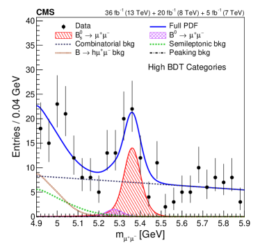
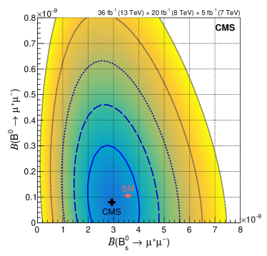
Figure 8: (left) Invariant dimuon mass distribution for the high BDT categories (cf. Table 5), with the fit projections overlaid. The peaking background is virtually invisible. (right) Likelihood contours of the branching fraction fit for ${\overline{\mathcal{B}}}(B^{0}_{s}\rightarrow\mu^{+}\mu^{-})$ and ${\mathcal{B}}(B^{0}\rightarrow\mu^{+}\mu^{-})$, with the best-fit value (black cross) and the SM expectation (red solid square).

For the determination of the $B^{0}_{s}\rightarrow\mu^{+}\mu^{-}$ effective lifetime $\tau_{\mu^{+}\mu^{-}}$, two independent fit frameworks were established, a 2D unbinned maximum likelihood fit to the invariant mass and decay time distributions and a 1D binned maximum likelihood fit to the decay time distribution where the background is subtracted with the sPlot method [32]. Prior to unblinding the data, the former was chosen as the primary method based on its better median expected performance. The fits are performed for the decay time range $1<t<11\mbox{\,ps}$ in eight BDT categories provided in Table 5. The decay time restriction is motivated by the very low selection efficiency at smaller decay times $t$, because of the $\ell_{3D}/\sigma(\ell_{3D})$ and isolation requirements, while the efficiency at large $t$ is strongly decreasing in Run 2, due to HLT requirements on the muon impact parameter. Concerns regarding the fit stability, given the small expected number of signal events, motivated using eight instead of 14 BDT categories.

The PDFs for the invariant mass of the 2D unbinned maximum likelihood fit are very similar to those in the branching fraction fits with the notable exception that $B^{0}\rightarrow\mu^{+}\mu^{-}$ is included in the peaking background. In the decay time PDFs, the exponential functions are convolved with Gaussian functions to account for detector resolution. The decay time efficiency is included in all fit components except for the combinatorial background, because its PDF is modeled from data directly. In the fit, the $B^{0}_{s}\rightarrow\mu^{+}\mu^{-}$ effective lifetime $\tau_{\mu^{+}\mu^{-}}$, the signal yield, and the parameters of the combinatorial background are floated (cf. Table 5 for a summary). All other parameters are constrained or fixed to the MC simulation values. There is no common ${\overline{\mathcal{B}}}(B^{0}_{s}\rightarrow\mu^{+}\mu^{-})$ constraint for the $B^{0}_{s}\rightarrow\mu^{+}\mu^{-}$ signal yields in the eight BDT categories. The result of the fit is

$$\tau_{\mu^{+}\mu^{-}}(B^{0}_{s}\rightarrow\mu^{+}\mu^{-})=1.70\,^{+0.61}_{-0.44}\,\mbox{\,ps},$$ (6)

where the error combines the large statistical (${}^{+0.60}_{-0.43}\mbox{\,ps}$) and small systematic ($\pm 0.09\mbox{\,ps}$) uncertainty. In Fig. 9 (left) the decay time distribution is shown, together with the fit results overlaid. The observed errors are about one root-mean-square deviation larger than expected (${}^{+0.39}_{-0.30}\mbox{\,ps}$). This is attributed to fluctuations in the small sample size.

The second determination of $\tau_{\mu^{+}\mu^{-}}$ uses the complete model of the branching fraction fit to determine the sPlot weights. An exponential function, modified to include the channel-dependent resolution and efficiency effects, is fit to the sPlot distribution. Special care is applied to determine asymmetric uncertainties and to reduce the bias due to the large bin widths. The fit yields $\tau_{\mu^{+}\mu^{-}}=1.55\ ^{+0.52}_{-0.33}\mbox{\,ps}$, where a fit bias of $+0.09\mbox{\,ps}$ has been corrected for. This bias, together with the dependence on the Run 2 data-taking periods, is the largest systematic error in this approach. The two determinations of the effective lifetime are consistent with each other.

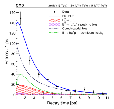
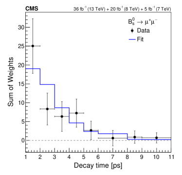
Figure 9: Decay time distributions for (left) the 2D unbinned maximum likelihood fit and (right) the sPlot fit approach. The data combine all events in the eight BDT categories of Table 5 (right part). In the left plot, the total fit is shown by the solid line, the signal by the single-hatched distribution, and the different background components by the broken lines and the cross-hatched distributions. In the right plot, only the signal component is shown as the background has been subtracted beforehand with the sPlot method (see text for details).

6 Conclusions

The CMS experiment has analyzed rare leptonic $B\rightarrow\mu^{+}\mu^{-}$ decays with 61$\mbox{\,fb}^{-1}$ of data collected in LHC Run 1 and 2016. The decay $B^{0}_{s}\rightarrow\mu^{+}\mu^{-}$ is observed with a significance of $5.6\,\sigma$ ($6.5\,\sigma$ expected). Its branching fraction is measured to be ${\overline{\mathcal{B}}}(B^{0}_{s}\rightarrow\mu^{+}\mu^{-})=[2.9\pm{0.7}\,(\text{exp})\pm{0.2}\,(\text{frag})]\times 10^{-9}$ and the $B^{0}_{s}\rightarrow\mu^{+}\mu^{-}$ effective lifetime is determined to be $\tau_{\mu^{+}\mu^{-}}=1.70\,^{+0.61}_{-0.44}\mbox{\,ps}$. Both results are limited by the small signal sample. No evidence is found for $B^{0}\rightarrow\mu^{+}\mu^{-}$ and an upper limit of ${\mathcal{B}}(B^{0}\rightarrow\mu^{+}\mu^{-})<3.6\times 10^{-10}$ (at 95% confidence level) is determined. These results are consistent with the SM. The branching fraction results are also consistent with the previous CMS analysis [12] when restricting this analysis to the Run 1 dataset.

References

- [1] C. Bobeth, M. Gorbahn, T. Hermann, M. Misiak, E. Stamou and M. Steinhauser, Phys. Rev. Lett. 112, 101801 (2014), arXiv:1311.0903 [hep-ph].
- [2] T. Hermann, M. Misiak and M. Steinhauser, JHEP 12, 097 (2013), arXiv:1311.1347 [hep-ph].
- [3] C. Bobeth, M. Gorbahn and E. Stamou, Phys. Rev. D 89, 034023 (2014), arXiv:1311.1348 [hep-ph].
- [4] M. Beneke, C. Bobeth and R. Szafron, Phys. Rev. Lett. 120, 011801 (2018), arXiv:1708.09152 [hep-ph].
- [5] M. Beneke, C. Bobeth and R. Szafron, JHEP 10, 232 (2019), arXiv:1908.07011 [hep-ph].
- [6] N. Cabibbo, Phys. Rev. Lett. 10, 531 (1963).
- [7] M. Kobayashi and T. Maskawa, Prog. Theor. Phys. 49, 652 (1973).
- [8] Particle Data Group, M. Tanabashi et al., Phys. Rev. D 98, 030001 (2018).
- [9] K. De Bruyn, R. Fleischer, R. Knegjens, P. Koppenburg, M. Merk and N. Tuning, Phys. Rev. D 86, 014027 (2012), arXiv:1204.1735 [hep-ph].
- [10] Flavour Lattice Averaging Group Collaboration, S. Aoki et al., Eur. Phys. J. C 80, 113 (2020), arXiv:1902.08191 [hep-lat].
- [11] ATLAS Collaboration, M. Aaboud et al., JHEP 04, 098 (2019), arXiv:1812.03017 [hep-ex].
- [12] CMS Collaboration, S. Chatrchyan et al., Phys. Rev. Lett. 111, 101804 (2013), arXiv:1307.5025 [hep-ex].
- [13] LHCb Collaboration, R. Aaij et al., Phys. Rev. Lett. 111, 101805 (2013), arXiv:1307.5024 [hep-ex].
- [14] LHCb Collaboration, R. Aaij et al., Phys. Rev. Lett. 118, 191801 (2017), arXiv:1703.05747 [hep-ex].
- [15] CMS Collaboration, A. M. Sirunyan et al., JHEP 04, 188 (2020), arXiv:1910.12127 [hep-ex].
- [16] D0 Collaboration, V. Abazov et al., Phys. Rev. Lett. 94, 071802 (2005), arXiv:hep-ex/0410039.
- [17] LHCb Collaboration, R. Aaij et al., Phys. Rev. Lett. 124, 122002 (2020), arXiv:1910.09934 [hep-ex].
- [18] ATLAS Collaboration, G. Aad et al., Phys. Rev. Lett. 115, 262001 (2015), arXiv:1507.08925 [hep-ex].
- [19] LHCb Collaboration, R. Aaij et al., Phys. Rev. D 100, 031102 (2019), arXiv:1902.06794 [hep-ex].
- [20] CMS Collaboration, S. Chatrchyan et al., JINST 3, S08004 (2008).
- [21] CMS Collaboration, V. Khachatryan et al., Eur. Phys. J. C 70, 1165 (2010), arXiv:1007.1988 [physics.ins-det].
- [22] CMS Collaboration, CMS Collaboration, Tracking POG results for pion efficiency with the meson using data from 2016 and 2017, CMS Detector Performance Note CMS-DP-2018-050 (2018).
- [23] CMS Collaboration, S. Chatrchyan et al., JINST 7, P10002 (2012), arXiv:1206.4071 [physics.ins-det].
- [24] CMS Collaboration, A. M. Sirunyan et al., JINST 13, P06015 (2018), arXiv:1804.04528 [physics.ins-det].
- [25] CMS Collaboration, V. Khachatryan et al., JINST 12, P01020 (2017), arXiv:1609.02366 [physics.ins-det].
- [26] H. Voss, A. Höcker, J. Stelzer and F. Tegenfeldt, TMVA, the toolkit for multivariate data analysis with ROOT, in XIth International Workshop on Advanced Computing and Analysis Techniques in Physics Research (ACAT), (2007). p. 40. arXiv:physics/0703039. [PoS(ACAT)040].
- [27] M. J. Oreglia, A study of the reactions , PhD thesis, Stanford University, (1980). SLAC-R-236, UMI-81-08973. See Appendix D.
- [28] K. S. Cranmer, Comput. Phys. Commun. 136, 198 (2001), arXiv:hep-ex/0011057 [hep-ex].
- [29] S. S. Wilks, Annals Math. Statist. 9, 60 (1938).
- [30] A. L. Read, J. Phys. G 28, 2693 (2002).
- [31] T. Junk, Nucl. Instrum. Meth. A 434, 435 (1999), arXiv:hep-ex/9902006.
- [32] M. Pivk and F. R. Le Diberder, Nucl. Instrum. Meth. A 555, 356 (2005), arXiv:physics/0402083 [physics.data-an].