Lagrangian dynamics
by nonlocal constants of motion

Abstract

A simple general theorem is used as a tool that generates nonlocal constants of motion for Lagrangian systems. We review some cases where the constants that we find are useful in the study of the systems: the homogeneous potentials of degree $-2$, the mechanical systems with viscous fluid resistance and the conservative and dissipative Maxwell-Bloch equations of laser dynamics. We also prove a new result on explosion in the past for mechanical system with hydraulic (quadratic) fluid resistance and bounded potential.

Gianluca Gorni

Università di Udine

Dipartimento di Scienze Matematiche, Informatiche e Fisiche

via delle Scienze 208, 33100 Udine, Italy

gianluca.gorni@uniud.it

Gaetano Zampieri

Università di Verona

Dipartimento di Informatica

strada Le Grazie 15, 37134 Verona, Italy

gaetano.zampieri@univr.it

1 Introduction

Consider the finite-dimensional variational Euler-Lagrange equation

$$\frac{d}{dt}\partial_{\dot{q}}L\bigl{(}t,q(t),\dot{q}(t)\bigr{)}-\partial_{q}L\bigl{(}t,q(t),\dot{q}(t)\bigr{)}=0\,,$$ (1)

where the Lagrangian $L(t,q,\dot{q})$ is a smooth function, with $t\in\mathbb{R}$, $q,\dot{q}\in\mathbb{R}^{n}$. We use the notation $\partial_{q}$ and $\partial_{\dot{q}}$ for the partial derivative operators with respect to the vector $q$ and $\dot{q}$ respectively, $\lvert x\rvert$ and $x\cdot y$ for the Euclidean norm and scalar product of vectors $x,y\in\mathbb{R}^{n}$.

A first integral is a smooth function of the form

$$N(t,q,\dot{q}),\qquad t\in\mathbb{R},\quad q,\dot{q}\in\mathbb{R}^{n},$$ (2)

that is constant along all solutions to Euler-Lagrange equation. The celebrated Noether’s theorem establishes a connection between first integrals and certain invariance properties of the Lagrangian function $L$.

A previous work of ours [3] revisited Noether’s Theorem from different points of view, including asynchronous perturbations (or “time change”) and boundary terms, this last being a nomenclature recommended by Leach [8]. In the present paper we focus on the extension we obtained to constants of motion of the more general form

$$N\bigl{(}t,q(t),\dot{q}(t)\bigr{)}+\int_{t_{0}}^{t}M\bigl{(}s,q(s),\dot{q}(s)\bigr{)}ds\,,$$ (3)

which we call nonlocal, because its value at a time $t$ depends not only on the value of position and velocity at time $t$, but also on the past history of the motion.

In later works (see, e.g., [6]) we extended the results to the nonvariational case, where an extra term $Q$ appears on the right-hand side of the differential equation, as in formula (4) below. For such systems the motions are not stationary points of the action functional associated with the Lagrangian $L$, in the sense of the calculus of variations.

The basic, very simple result on nonlocal constants of motion in that paper [6] can be reformulated in the following self-contained way, which is all that is needed for the sequel:

Theorem 1.

Let $t\mapsto q(t)$ be a solution to the Lagrange equation

$$\frac{d}{dt}\partial_{\dot{q}}L\bigl{(}t,q(t),\dot{q}(t)\bigr{)}-\partial_{q}L\bigl{(}t,q(t),\dot{q}(t)\bigr{)}=Q\bigl{(}t,q(t),\dot{q}(t)\bigr{)}$$ (4)

for smooth $L(t,q,\dot{q})$, $Q(t,q,\dot{q})$, with $t\in\mathbb{R}$, $q,\dot{q}\in\mathbb{R}^{n}$, and let $q_{\lambda}(t)$, $\lambda\in\mathbb{R}$, be a smooth family of perturbed motions, such that $q_{0}(t)\equiv q(t)$. Then the following function is constant:

$$t\mapsto\boxed{\partial_{\dot{q}}L\bigl{(}t,q(t),\dot{q}(t)\bigr{)}\cdot\partial_{\lambda}q_{\lambda}(t)\big{|}_{\lambda=0}-\int_{t_{0}}^{t}\biggl{(}\frac{\partial}{\partial\lambda}L\bigl{(}s,q_{\lambda}(s),\dot{q}_{\lambda}(s)\bigr{)}\big{|}_{\lambda=0}+{}}\\ \boxed{{}+Q\bigl{(}s,q(s),\dot{q}(s)\bigr{)}\cdot\partial_{\lambda}q_{\lambda}(s)\big{|}_{\lambda=0}\biggr{)}ds}\,.$$ (5)

Proof.

Take $\frac{d}{dt}$ of (5), and use (4) and $\frac{d}{dt}\partial_{\lambda}q_{\lambda}(t)=\partial_{\lambda}\dot{q}_{\lambda}(t)$ at $\lambda=0$. ∎

The constant (5) is often trivial or of no apparent practical value, but there are cases when it is interesting and useful. In the rest of this paper we will review some applications in the variational case

• potentials with simple symmetries in Section 2 as basic motivation,

• homogeneous potentials of degree $-2$ in Section 3, taken from [3],

• viscous fluid resistance in Section 4, taken from [4],

and two in the nonvariational case:

• hydraulic fluid resistance in Section 5,

• the Maxwell-Bloch equations for laser dynamics in Section 6, taken from [5] in the conservative case and from [6] and [7] in the dissipative case.

The result in Section 5 is actually new: for a particle in $\mathbb{R}^{n}$ under quadratic fluid resistance and a bounded, nonnegative potential energy, we prove the explosion in the past in finite time of all solutions with initial kinetic energy greater than the upper bound of the potential energy.

2 Lagrangians with simple symmetries

The perturbed motions $q_{\lambda}(t)$ of Theorem 1 were originally inspired by the mechanism that Noether’s theorem uses to deduce conservation laws for variational Lagrangian systems (for which $Q\equiv 0$) under certain symmetry conditions on $L$. A simple example is a particle of mass $m$ in the plane that is driven by a central force field

$$L(t,q,\dot{q}):=\frac{1}{2}m\lvert\dot{q}\rvert^{2}-U\bigl{(}t,\lvert q\rvert\bigr{)},\quad q=(q_{1},q_{2})\in\mathbb{R}^{2}.$$ (6)

To exploit the rotational symmetry of $L$ it is natural to take the rotation family

$$q_{\lambda}(t):=\begin{pmatrix}\cos\lambda&-\sin\lambda\\ \sin\lambda&\cos\lambda\end{pmatrix}q(t),\qquad\partial_{\lambda}q_{\lambda}(t)\big{|}_{\lambda=0}=\bigl{(}-q_{2}(t),q_{1}(t)\bigr{)}\,.$$ (7)

It is clear that $L(t,q_{\lambda}(t),\dot{q}_{\lambda}(t))$ does not depend on $\lambda$. Formula (5) reduces to a simple version of Noether’s theorem and gives the angular momentum as constant of motion:

$$\partial_{\dot{q}}L\cdot\partial_{\lambda}q_{\lambda}\big{|}_{\lambda=0}=m\dot{q}\cdot(-q_{2},q_{1})=m(q_{1}\dot{q}_{2}-q_{2}\dot{q}_{1}).$$

A simple, somewhat less conventional use of the theorem is the following. For time independent $L(t,q,\dot{q})=\mathcal{L}(q,\dot{q})$, $Q\equiv 0$, and the time-shift family $q_{\lambda}(t)=q(t+\lambda)$ we have

$$\partial_{\lambda}L\bigl{(}t,q_{\lambda}(t),\dot{q}_{\lambda}(t)\bigr{)}\big{|}_{\lambda=0}=\partial_{q}\mathcal{L}\cdot\dot{q}(t)+\partial_{\dot{q}}\mathcal{L}\cdot\ddot{q}(t).$$

The constant of motion is

$$\partial_{\dot{q}}\mathcal{L}\cdot\dot{q}(t)-{} \int_{t_{0}}^{t}\frac{d}{ds}\mathcal{L}\bigl{(}q(s),\dot{q}(s)\bigr{)}ds=$$

$$=\partial_{\dot{q}}\mathcal{L}\bigl{(}q(t),\dot{q}(t)\bigr{)}\cdot\dot{q}(t)-\mathcal{L}\bigl{(}q(t),\dot{q}(t)\bigr{)}+\mathcal{L}\bigl{(}q(t_{0}),\dot{q}(t_{0})\bigr{)}=$$

$$=E\bigl{(}q(t),\dot{q}(t)\bigr{)}+\mathcal{L}\bigl{(}q(t_{0}),\dot{q}(t_{0})\bigr{)},$$

which coincides with the energy

$$E(q,\dot{q})=\partial_{\dot{q}}\mathcal{L}(q,\dot{q})\cdot\dot{q}-\mathcal{L}(q,\dot{q})$$ (8)

up to the additive constant $\mathcal{L}(q(t_{0}),\dot{q}(t_{0}))$. For instance, when the Lagrangian is $\mathcal{L}(q,\dot{q}):=\frac{1}{2}m\lvert\dot{q}\rvert^{2}-U(q)$, the conserved energy takes the classical form of kinetic plus potential energies: $E(q,\dot{q})=\frac{1}{2}m\lvert\dot{q}\rvert^{2}+U(q)$.

3 Homogeneous potentials of degree $-2$

In this section we are going to review a result in our previous work [3], Section 9. Consider the variational mechanical system of a point moving in a potential field:

$$L(t,q,\dot{q}):=\frac{1}{2}m\lvert\dot{q}\rvert^{2}-U(q),\qquad Q\equiv 0,\qquad m\ddot{q}=-\nabla U(q),$$ (9)

and assume that the potential $U$ is positively homogeneous of degree $-2$:

$$U(sq)=s^{-2}U(q),\qquad\forall s>0.$$ (10)

Two notable examples are the central potential case

$$U(q)=-k/|q|^{2},\qquad q\in\mathbb{R}^{n}\setminus\{0\},$$ (11)

and Calogero’s potential

$$U(q_{1},\dots,q_{n})=g^{2}\sum_{1\leq j<k\leq n}(q_{j}-q_{k})^{-2},$$

for $q_{j}\in\mathbb{R}$, $q_{j}\neq q_{k}$ when $j\neq k$, see Calogero’s paper [2].

All these systems enjoy a remarkable symmetry: if $q(t)$ is solution to the last of (9), then

$$q_{\lambda}(t)=e^{\lambda}q\bigl{(}e^{-2\lambda}t\bigr{)},$$

is a solution too. Theorem 1 associates to this family $q_{\lambda}$ the following constant of motion

$$K={} \partial_{\dot{q}}L\cdot\partial_{\lambda}q_{\lambda}(t)\big{|}_{\lambda=0}-\int\frac{\partial}{\partial\lambda}L\bigl{(}t,q_{\lambda}(t),\dot{q}_{\lambda}(t)\bigr{)}\big{|}_{\lambda=0}dt=$$

$$={} m\dot{q}\cdot(q-2t\dot{q})-2tU=m\dot{q}\cdot(q-2t\dot{q})+2tL.$$

This time-dependent local constant of motion can be rewritten in terms of the energy $E$, which is constant too:

$$K=m\dot{q}\cdot q-2tE,\qquad E:=\frac{1}{2}m\lvert\dot{q}\rvert^{2}+U(q).$$

Take the antiderivative in time of $0=mq\cdot\dot{q}-2tE-K$ and obtain one more constant of motion

$$K_{1}=\frac{1}{2}m\lvert q\rvert^{2}-t^{2}E-tK\,.$$

We can solve for $\lvert q\rvert$:

$$\bigl{|}q(t)\bigr{|}=\sqrt{\frac{2}{m}}\sqrt{t^{2}E+tK+K_{1}}\,.$$ (12)

This formula gives the explicit time-dependence of the distance from the origin, even though we don’t know the shape of the orbit.

4 Viscous fluid resistance

This Section reviews the main result of our paper [4]. Consider a particle under a bounded from below potential $U\colon\mathbb{R}^{n}\to\mathbb{R}$ and viscous (linear) fluid resistance:

$$m\ddot{q}=-k\dot{q}-\nabla U(q),\qquad U\geq 0,\quad q\in\mathbb{R}^{n},$$ (13)

where $m$ and $k>0$ are parameters. The mechanical energy

$$\frac{1}{2}m\lvert\dot{q}\rvert^{2}+U(q)$$ (14)

decreases along solutions $q(t)$ and $\dot{q}(t)$ is bounded in the future:

$$\frac{1}{2}m\bigl{|}\dot{q}(t)\bigr{|}^{2}\leq\frac{1}{2}m\bigl{|}\dot{q}(t_{0})\bigr{|}^{2}+U\bigl{(}q(t_{0})\bigr{)},\qquad t\geq t_{0}.$$

So $q(t)$ is bounded for bounded $t$ and we get global existence in the future. What about the past? Equation (13) can be put into Lagrangian form (4) with

$$L(t,q,\dot{q}):=e^{kt/m}\Bigl{(}\frac{1}{2}m\lvert\dot{q}\rvert^{2}-U(q)\Bigr{)},\qquad Q\equiv 0.$$

Incidentally, a study of Noether symmetries and conservation laws for this Lagrangian function has been made by Leone and Gourieux [9].

Let us apply Theorem 1 with the family $q_{\lambda}(t):=q(t+\lambda e^{kt/m})$. Then computing the nonlocal constant of motion (5) and integrating by parts we have a simple formula for the constant of motion:

$$e^{2kt/m}\Bigl{(}m\lvert\dot{q}(t)\rvert^{2}+2U\bigl{(}q(t)\bigr{)}\Bigr{)}-\frac{4k}{m}\int^{t}_{t_{0}}e^{2ks/m}U\bigl{(}q(s)\bigr{)}ds.$$

Since $U\geq 0$, the integral term increases with $t$, forcing the remaining part

$$e^{2kt/m}\Bigl{(}m\lvert\dot{q}(t)\rvert^{2}+2U\bigl{(}q(t)\bigr{)}\Bigr{)}$$

to be increasing too. We deduce the inequalities

$$me^{2kt/m}\lvert\dot{q}(t)\rvert^{2}\leq{} e^{2kt/m}\Bigl{(}\lvert\dot{q}(t)\rvert^{2}+2U\bigl{(}q(t)\bigr{)}\Bigr{)}\leq$$ (15)

$$\leq{} e^{2kt_{0}/m}\Bigl{(}\lvert\dot{q}(t_{0})\rvert^{2}+2U\bigl{(}q(t_{0})\bigr{)}\Bigr{)}\qquad\forall t\leq t_{0}.$$ (16)

In a bounded interval $(t_{1},t_{0}]$ the velocity $\dot{q}(t)$ is bounded, and therefore $q(t)$ is too. This proves global existence of solutions also in the past.

5 Explosion in the past for hydraulic fluid resistance

We are going to see a new result. Consider the equation for hydraulic resistance in a bounded potential field:

$$m\ddot{q}=-k\lvert\dot{q}\rvert\dot{q}-\nabla U\bigl{(}q(t)\bigr{)},\quad q\in\mathbb{R}^{n},$$ (17)

where $m,k>0$ are parameters, and the smooth potential is bounded:

$$0\leq U(q)\leq U_{\sup}<+\infty\qquad\forall q\in\mathbb{R}^{n}.$$ (18)

The same argument as in the previous section shows that we have global existence in the future.

We cannot expect global existence in the past already in the simple one-dimensional example $m\ddot{q}=-k\lvert\dot{q}\rvert\dot{q}$, $q\in\mathbb{R}$, for which all nonconstant solutions are of the form $q(t)=\frac{m}{k}\log(\omega(t-t_{0}))$, for parameters $\omega>0$, $t_{0}\in\mathbb{R}$, which are only defined for $t>t_{0}$.

To investigate possible non-globality in the past in the general case of hydraulic resistance in a bounded potential field, let us put this system into the Lagrange nonvariational formulation (4) with the choices

$$L(t,q,\dot{q}):=\frac{1}{2}m\lvert\dot{q}\rvert^{2}-U(q),\qquad Q(t,q,\dot{q}):=-k\dot{q}\lvert\dot{q}\rvert.$$ (19)

If we take the family $q_{\lambda}(t):=q(t+\lambda e^{-at})$, with $a>0$, from formula (5), we obtain the following constant of motion:

$$e^{-at}m\lvert\dot{q}(t)\rvert^{2}+\int_{t_{0}}^{t}e^{-as}\Bigl{(}\lvert\dot{q}(s)\rvert^{3}+am\lvert\dot{q}(s)\rvert^{2}+\nabla U\bigl{(}q(s)\bigr{)}\cdot\dot{q}(s)-m\ddot{q}(s)\cdot\dot{q}(s)\Bigr{)}ds,$$ (20)

which can be rewritten, after a couple of integrations by parts, as

$$\frac{m}{2}e^{-at}\lvert\dot{q}(t)\rvert^{2}+e^{-at}U\bigl{(}q(t)\bigr{)}-e^{-at_{0}}U\bigl{(}q(t_{0})\bigr{)}+\\ +\frac{1}{2}\int_{t_{0}}^{t}e^{-as}\Bigl{(}2k\lvert\dot{q}(s)\rvert^{3}+am\lvert\dot{q}(s)\rvert^{2}+2aU\bigl{(}q(s)\bigr{)}\Bigr{)}ds\equiv\frac{m}{2}e^{-at_{0}}\lvert\dot{q}(t_{0})\rvert^{2}.$$ (21)

Crucially, the left-hand side is monotonic with respect to the value of $\lvert\dot{q}\rvert$.

When $t<t_{0}$, from (21) and (18) we can write the inequality

$$\frac{m}{2}e^{-at_{0}}\lvert\dot{q}(t_{0})\rvert^{2}\equiv{} \frac{m}{2}e^{-at}\lvert\dot{q}(t)\rvert^{2}+e^{-at}U\bigl{(}q(t)\bigr{)}-e^{-at_{0}}U\bigl{(}q(t_{0})\bigr{)}+{}$$

$${}+\frac{1}{2}\int_{t_{0}}^{t}e^{-ks}\Bigl{(}2k\lvert\dot{q}(s)\rvert^{3}+am\lvert\dot{q}(s)\rvert^{2}+2aU\bigl{(}q(s)\bigr{)}\Bigr{)}ds\leq$$

$$\leq{} \frac{m}{2}e^{-at}\lvert\dot{q}(t)\rvert^{2}+e^{-at}U_{\sup}+{}$$ (22)

$${}+\frac{1}{2}\int_{t_{0}}^{t}e^{-as}\Bigl{(}2k\lvert\dot{q}(s)\rvert^{3}+am\lvert\dot{q}(s)\rvert^{2}\Bigr{)}ds.$$ (23)

We wish to compare the smooth scalar function $t\mapsto\lvert\dot{q}(t)\rvert^{2}$ with the solution $z(t)$ of the integral equation

$$\frac{m}{2}e^{-at_{0}}\lvert\dot{q}(t_{0})\rvert^{2}\equiv\frac{m}{2}e^{-at}z(t)+e^{-at}U_{\sup}+\frac{1}{2}\int_{t_{0}}^{t}e^{-as}\Bigl{(}2k\bigl{|}z(s)\bigr{|}^{3/2}+az(s)\Bigr{)}ds,$$ (24)

which is equivalent to a Cauchy problem for a differential equation with separated variables:

$$\frac{z^{\prime}(t)}{kz(t)^{3/2}-aU_{\sup}}=-\frac{2}{m},$$ (25)

$$z(t_{0})=\lvert\dot{q}(t_{0})\rvert^{2}-\frac{2}{m}U_{\sup}.$$ (26)

Suppose that

$$\lvert\dot{q}(t_{0})\rvert^{2}>\frac{2U_{\sup}}{m}+\Bigl{(}\frac{aU_{\sup}}{k}\Bigr{)}^{2/3}\,,$$ (27)

so that $kz(t_{0})^{3/2}-aU_{\sup}>0$. Then the denominator in (25) is $>0$, $z(t)$ is decreasing and it explodes in the past at a finite time $t^{*}<t_{0}$ given by integrating the differential equation:

$$\int_{z(t_{0})}^{+\infty}\frac{du}{ku^{3/2}-aU_{\sup}}=-\frac{2}{m}(t^{*}-t_{0}).$$ (28)

The inequality $z(t)<\lvert\dot{q}(t)\rvert^{2}$ holds in a neighbourhood of $t=t_{0}$. To prove that it holds for all $t\in\mathopen{]}t^{*},t_{0}]$, suppose that there exists a time $t_{1}<0$ such that $z(t_{1})=\lvert\dot{q}(t_{1})\rvert^{2}$ and that $z(t)<\lvert\dot{q}(t)\rvert^{2}$ holds for all $t\in\mathopen{]}t_{1},t_{0}]$. Then we can concatenate (23) with (24):

$$\frac{m}{2}e^{-at_{0}}{} \lvert\dot{q}(t_{0})\rvert^{2}\leq{}$$

$$\leq{} \frac{m}{2}e^{-at_{1}}\lvert\dot{q}(t_{1})\rvert^{2}+e^{-at_{1}}U_{\sup}+\frac{1}{2}\int_{t_{0}}^{t_{1}}e^{-as}\Bigl{(}2k\lvert\dot{q}(s)\rvert^{3}+a\lvert\dot{q}(s)\rvert^{2}\Bigr{)}ds=$$

$$={} \frac{m}{2}e^{-at_{1}}z(t_{1})+e^{-at_{1}}U_{\sup}+\frac{1}{2}\int_{t_{0}}^{t_{1}}e^{-as}\Bigl{(}2k\lvert\dot{q}(s)\rvert^{3}+a\lvert\dot{q}(s)\rvert^{2}\Bigr{)}ds<$$

$$<{} \frac{m}{2}e^{-at_{1}}z(t_{1})+e^{-at_{1}}U_{\sup}+\frac{1}{2}\int_{t_{0}}^{t_{1}}e^{-as}\Bigl{(}2k\lvert z(s)\rvert^{3/2}+az(s)\Bigr{)}ds=$$

$$={} \frac{m}{2}e^{-at_{0}}\lvert\dot{q}(t_{0})\rvert^{2},$$

which is impossible. We conclude that, for $t<t_{0}$, $\lvert\dot{q}(t)\rvert^{2}$ is controlled from below, as long as it exists, by a function $z(t)$ that explodes to $+\infty$ in finite time. Since the constant $a>0$ can be chosen arbitrarily small, the inequality (27) can be replaced by $\lvert\dot{q}(t_{0})\rvert^{2}>2U_{\sup}/m$, which is nicely equivalent to $\frac{m}{2}\lvert\dot{q}(t_{0})\rvert^{2}>U_{\sup}$.

Conclusion: if $0\leq U\leq U_{\sup}<+\infty$, all the solutions to the differential equation (17) for which the initial kinetic energy $\frac{m}{2}\lvert\dot{q}(t_{0})\rvert^{2}$ is strictly greater than $U_{\sup}$ explode in the past in finite time.

6 The Maxwell-Bloch equations

The Maxwell-Bloch equations are well-known to describe laser dynamics for a system of two-level atoms in a cavity resonator. They were first derived in a 1965 paper by Arecchi et Bonifacio. The so called resonant case can be written as

$$\begin{cases}\ddot{q}_{1}=-abq_{1}-(a+b)\dot{q}_{1}+g^{2}q_{1}\dot{q}_{3}\\ \ddot{q}_{2}=-abq_{2}-(a+b)\dot{q}_{2}+g^{2}q_{2}\dot{q}_{3}\\ \ddot{q}_{3}=-a\bigl{(}q_{1}^{2}+q_{2}^{2}\bigr{)}-c(\dot{q}_{3}-k)-\bigl{(}q_{1}\dot{q}_{1}+q_{2}\dot{q}_{2}\bigr{)},\end{cases}$$ (29)

which has the Lagrangian form (4) with the following choice of $L,Q$:

$$L=\frac{1}{2}\bigl{(}\dot{q}_{1}^{2}+\dot{q}_{2}^{2}+g^{2}\dot{q}_{3}^{2}+(q_{1}^{2}+q_{2}^{2})(g^{2}\dot{q}_{3}-ab\bigr{)}\bigr{)},$$ (30)

$$Q=-\Bigl{(}(a+b)\dot{q}_{1},(a+b)\dot{q}_{2},ag^{2}\bigl{(}q_{1}^{2}+q_{2}^{2}\bigr{)}+cg^{2}(\dot{q}_{3}-k)\Bigr{)},$$ (31)

where $a,b,c\geq 0$, $g>0$, $k\in\mathbb{R}$ are parameters (see Arecchi and Meucci [1] and our paper with Residori [7]). We are going to briefly describe two kinds of nonstandard separation of variables that hold when $a=b=c=0$ (conservative case) and when $a,b,c>0$ (dissipative) with $c=2a$. From these separations, we deduced or conjectured some dynamical features which we will not repeat here. All details are in our paper [5] in the conservative case, and in the already cited [7] in the dissipative case.

6.1 Conservative case $a=b=c=0$

Using the anisotropic scaling family

$$q_{\lambda}(t)=\bigl{(}e^{\lambda}q_{1}(t),e^{\lambda}q_{2}(t),e^{-2\lambda}q_{3}(t)\bigr{)}\,,$$ (32)

the constant of motion (5) becomes

$$\ddot{q}_{3}(t)+2Bg^{2}q_{3}(t)+2Et-3g^{2}\int_{t_{0}}^{t}\dot{q}_{3}(s)^{2}ds\,,$$ (33)

were $B,E$ are the known first integrals

$$E=\frac{1}{2}\bigl{(}\dot{q}_{1}^{2}+\dot{q}_{2}^{2}+g^{2}\dot{q}_{3}^{2}\bigr{)},\qquad B=\dot{q}_{3}+\frac{1}{2}(q_{1}^{2}+q_{2}^{2}).$$ (34)

By derivation of (33) with respect to $t$ we get the differential equation of order 2 for $z:=\dot{q}_{3}$

$$\ddot{z}(t)+2Bg^{2}z(t)+2E-3g^{2}z(t)^{2}=0.$$ (35)

which has two equilibria with a fish-shaped separatrix. From this well-known equation it is easy to classify the conditions for the solution in $z:=\dot{q}_{3}$ to be periodic or homoclinic, as shown in Fig. 1.

The $(q_{1},q_{2})$ obeys a central force dynamics. Indeed, plugging $\dot{q}_{3}=B-\frac{1}{2}r^{2}$, with $r^{2}=q_{1}^{2}+q_{2}^{2}$, into the first two Lagrange equations we have

$$\ddot{q}_{1}=g^{2}\Bigl{(}B-\frac{1}{2}r^{2}\Bigr{)}q_{1},\qquad\ddot{q}_{2}=g^{2}\Bigl{(}B-\frac{1}{2}r^{2}\Bigr{)}q_{2}.$$ (36)

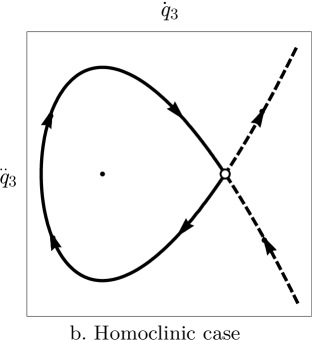
Figure 1: Generic (periodic) and homoclinic orbits of $(\dot{q}_{3},\ddot{q}_{3})$ in the conservative case of the Maxwell-Bloch equations (Subsec. 6.1); the dashed lines and the dots are not visited by solutions, but they are level sets or stationary points of the potential function associated with equation (35).

6.2 Dissipative case $a,b,c>0$

The family $q_{\lambda}(t)=q(t)+\lambda(0,0,2e^{ct})$ in (5) gives the constant of motion

$$g^{2}e^{ct}\bigl{(}q_{1}(t)^{2}+q_{2}(t)^{2}+2\dot{q}_{3}(t)-2k\bigr{)}+(2a-c)g^{2}\int e^{ct}\bigl{(}q_{1}(t)^{2}+q_{2}(t)^{2}\bigr{)}dt.$$

When $c=2a$ we have a first integral

$$M=e^{2at}\bigl{(}q_{1}^{2}+q_{2}^{2}+2\dot{q}_{3}-2k\bigr{)}\,,$$ (37)

which permits a separation of the $q_{1},q_{2}$ variables. In polar coordinates $(r,\theta)$ in the $q_{1},q_{2}$ plane we have

$$\ddot{r}=-(a+b)\dot{r}+\Bigl{(}g^{2}k-ab+\frac{g^{2}M}{2}e^{-2at}\Bigr{)}r-\frac{g^{2}}{2}r^{3}+\frac{N^{2}}{r^{3}}e^{-2(a+b)t},$$ (38)

$$N=e^{(a+b)t}r^{2}\dot{\theta},$$ (39)

where $N$ is another constant of motion which can be deduced from (5) with the rotation family

$$q_{\lambda}(t)=\bigl{(}q_{1}(t)\cos\lambda+q_{2}(t)\sin\lambda,-q_{1}(t)\sin\lambda+q_{2}(t)\cos\lambda,q_{3}(t)\bigr{)}.$$ (40)

We can solve for the remaining variable $q_{3}$ using the first integral $M$ of formula (37):

$$\dot{q}_{3}(t)=k-\frac{1}{2}r(t)^{2}+\frac{1}{2}Me^{-2at}.$$ (41)

Let us have a look at what happens if the time exponentials $e^{-2at}$ and $e^{-2(a+b)t}$ in equation (38) are replaced by their limit 0 as $t\to+\infty$:

$$\ddot{r}=-(a+b)\dot{r}+(g^{2}k-ab)r-\frac{g^{2}}{2}r^{3}.$$ (42)

This limiting equation has constant solutions corresponding to the nonnegative solutions of the algebraic equation

$$(g^{2}k-ab)r-\frac{g^{2}}{2}r^{3}=0.$$ (43)

There are clearly two cases:

• If $g^{2}k\leq ab$ then equation (43) has only the solution $r=0$. We conjecture that $r(t)\to 0$ for all solutions of the original equation (38). Figure 2a shows such a trajectory on the $q_{1},q_{2}$ plane.

• If $g^{2}k>ab$ we have two nonnegative solutions $r=0$ and

  $$r_{\infty}=\frac{1}{g}\sqrt{2(g^{2}k-ab)}.$$ (44)

  The conjecture is that the nontrivial solutions in the $q_{1},q_{2}$ plane converge to a point on the circle with radius $r_{\infty}$ and center in the origin, as in Figure 2b.

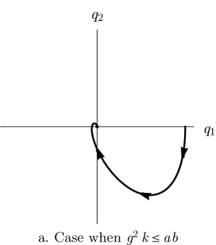
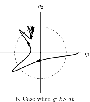
Figure 2: Projection of forward orbits on the $q_{1},q_{2}$ plane in two dissipative cases with $c=2a$ of the Maxwell-Bloch equations (Subsec. 6.2), computed numerically. On the left with $g^{2}k\leq ab$ the solution goes to the origin; on the right with $g^{2}k>ab$ the orbit converges to a point on the (dashed) circle with radius $r_{\infty}$, as in equation (44).

7 Conclusions

When studying mechanical systems with a Lagrangian structure, we think that it is worthwhile to apply Theorem 1 in search of useful integral constants of motion. At the moment the choice of the family $q_{\lambda}$ is more of an art, rather than a science. However, we hope this paper provides enough concrete examples to stimulate the curiosity of the reader.

References

[1]F. T. Arecchi and R. Meucci,
Chaos in lasers.
Scholarpedia 3(9):7066 (2008).
[2]F. Calogero,
Solutions of the one dimensional -body problems with quadratic and/or inversely quadratic pair potentials.
J. Math. Phys, 12 (1971),
419–436.
[3]G. Gorni and G. Zampieri,
Revisiting Noether’s theorem on constants of motion.
Journal of Nonlinear Mathematical Physics, 21,
No. 1 (2014), 43–73.
[4]G. Gorni and G. Zampieri,
Nonlocal variational constants of motion in dissipative dynamics.
Differential and Integral Equations, 30 (2017), 631–640.
[5]G. Gorni and G. Zampieri,
Nonstandard separation of variables for the Maxwell-Bloch conservative system.
São Paulo J. Math. Sci., 12, No. 1 (2018), 146–169.
[6]G. Gorni and G. Zampieri,
Nonlocal and nonvariational
extensions of Killing- type equations.
Discrete Contin. Dyn. Syst. Ser. S, 11, No. 4 (2018), 675–689.
[7]G. Gorni, S. Residori, G. Zampieri,
A quasi separable
dissipative Maxwell- Bloch system for laser dynamics.
Qual. Theory Dyn. Syst., 18, No. 2 (2019), 371–381.
[8]P. G. L. Leach,
Lie symmetries and Noether symmetries.
Applicable Analysis and Discrete Mathematics, 6 (2012),
238–246.
[9]R. Leone and T. Gourieux,
Classical Noether theory with application to the linearly damped particle.
European Journal of Physics, 36 (2015)
065022, 20pp.