LISA sources from young massive and open stellar clusters

Abstract

I study the potential role of young massive star clusters (YMCs) and open star clusters (OCs) in assembling stellar-mass binary black holes (BBHs) which would be detectable as persistent gravitational-wave (GW) sources by the forthcoming, space-based Laser Interferometer Space Antenna (LISA). The energetic dynamical interactions inside star clusters make them factories of assembling BBHs and other types of double-compact binaries that undergo general-relativistic (GR) inspiral and merger. The initial phase of such inspirals would, typically, sweep through the LISA GW band. This fabricates a unique opportunity to probe into the early in-spiralling phases of merging BBHs, that would provide insights into their formation mechanisms. Here, such LISA sources are studied from a set of evolutionary models of star clusters with masses ranging over $10^{4}M_{\odot}-10^{5}M_{\odot}$ that represent YMCs and intermediate-aged OCs in metal-rich and metal-poor environments of the Local Universe. These models are evolved with long-term, direct, relativistic many-body computations incorporating state-of-the-art stellar-evolutionary and remnant-formation models. Based on models of Local Universe constructed with such model clusters, it is shown that YMCs and intermediate-aged OCs would yield several 10s to 100s of LISA BBH sources at the current cosmic epoch with GW frequency within $10^{-3}{\rm~{}Hz}-10^{-1}{\rm~{}Hz}$ and signal-to-noise-ratio (S/N) $>5$, assuming a mission lifetime of 5 or 10 years. Such LISA BBHs would have a bimodal distribution in total mass, be generally eccentric ($\lesssim 0.7$), and typically have similar component masses although mass-asymmetric systems are possible. Intrinsically, there would be 1000s of present-day, LISA-detectable BBHs from YMCs and OCs. That way, YMCs and OCs would provide a significant and the dominant contribution to the stellar-mass BBH population detectable by LISA. A small fraction, $<5$%, of these BBHs would undergo GR inspiral to make it to LIGO-Virgo GW frequency band and merge, within the mission timespan; $<15$% would do so within twice the timespan. LISA BBH source counts for a range of S/N, normalized w.r.t. the local cluster density, are provided. Drawbacks in the present approach and future improvements are discussed.

I Introduction

Following the recent, above-the-expectation success of the LISA Pathfinder mission (Armano et al., 2016), Laser Interferometer Space Antenna (LISA; also, eLISA) has now been approved as an L3 mission by the European Space Agency (Amaro-Seoane et al., 2017). LISA is a proposed space-borne, dual-arm interferometer gravitational wave (hereafter GW) detector with an arm length of $2.5\times 10^{6}$ km. Such arm length makes the instrument sensitive to GWs of much lower frequencies, $\sim 10^{-5}-10^{-1}{\rm~{}Hz}$ (Amaro-Seoane et al., 2017), compared to its ground-based counterparts (Abadie et al., 2010; Abbott et al., 2016). LISA will thus potentially observe a wide-variety of low-frequency GW events such as mergers of binary supermassive black holes, inspiral and mergers of binary intermediate-mass black holes, intermediate mass ratio and extreme mass ratio inspirals involving supermassive and intermediate-mass black holes, Galactic binary white dwarfs and binary stars, and stellar-remnant binary black holes (hereafter BBH) and other double-compact binaries in the Local Universe (Amaro-Seoane et al., 2017, 2007; Ruiter et al., 2010; Holley-Bockelmann and Khan, 2015; Sesana, 2016).

Over their first (O1), second (O2), and third (O3) observing runs, the LIGO-Virgo collaboration (hereafter LVC) has identified 67 compact-binary merger events, which are predominantly BBH merger candidates but also contain binary neutron star (hereafter BNS) and neutron star-black hole (hereafter NSBH) merger events. Among these, the parameter estimations of 11 BBH mergers and 2 BNS mergers have so far been published (Abbott et al. (2019, 2020); The LIGO Scientific Collaboration and the Virgo Collaboration (2020), https://gracedb.ligo.org/superevents/public/O3/). However, various theories leading to compact-binary mergers and their observed properties (see Benacquista and Downing (2013) for a review) still remain largely degenerate.

One of the main reasons for this degeneracy is the fact that most compact binaries “forget” their orbital parameters at formation and hence the imprints of their formation mechanisms, by shrinking to a large extent and becoming practically circular by the time they spiral in, via GW radiation, up to the LIGO-Virgo GW frequency band ($\sim 10-1000$ Hz). By probing BBHs and other double-compact binaries at GW frequencies that are lower by a few orders of magnitude, LISA has the potential to identity imprints of such systems’ formation mechanisms. In that sense, identification of BBHs and other double-compact binaries by LISA and as well by other proposed, deci-Hertz-range, space-based GW interferometers such as DECIGO (Kawamura et al., 2008; Arca Sedda et al., 2019) and Tian Qin (Luo et al., 2016; Liu et al., 2020) would be complementary to the ground-based general-relativistic (hereafter GR) merger detections.

In particular, it can generally be expected that BBHs assembled via dynamical interactions in stellar clusters would be eccentric. Dynamically-formed BBHs that merge within a Hubble time would exhibit relics of this eccentricity in the LISA frequency band (Nishizawa et al., 2016, 2017), on their way to the merger via post-Newtonian (hereafter PN) inspiral. Detailed and self-consistent direct N-body and Monte Carlo simulations of young, open, and globular clusters indeed support this (Banerjee, 2018a; Kremer et al., 2019; Banerjee, 2020). In contrast, isolated binary evolution can be expected to produce predominantly circular BBHs in the LISA band. This is because to place a BBH, derived from massive stellar binary evolution, in the LISA band, the binary must go through a common-envelope (CE) phase (Ivanova et al., 2013) so that it shrinks sufficiently (Belczynski et al., 2016a; Mandel and Farmer, 2017; Stevenson et al., 2017; Giacobbo et al., 2018; Baibhav et al., 2019), which process would also circularize them. Except for the least massive merging BBHs produced in this way (which would also have the least chances to be visible by LISA), that may become eccentric at the beginning of their GR-inspiral due to BHs’ natal kick (Banerjee et al., 2020) (especially, that of the later-born BH), the BH members would form via direct collapse without any natal kick, preserving the circular binary orbit .

Note that the typical timescale of PN orbital evolution of BBHs in the LISA band is $\sim 0.1$ Myr although, depending on the BBH’s orbital configuration, it can be as small as $\sim 10$ yr (Banerjee, 2020). Therefore, BBHs in the LISA band are persistent or semi-persistent GW sources. In contrast, they are transient GW sources in the LIGO-Virgo band, the inspiral timescale being $\lesssim$ a minute.

The contribution of BBH LISA sources from globular clusters (hereafter GC) and nuclear clusters (hereafter NSC) in the Local Universe, due to dynamical processes in such clusters, has recently been studied (Samsing and D’Orazio, 2018; Kremer et al., 2019; Hoang et al., 2019). This study investigates BBH LISA sources from young massive clusters (hereafter YMC) and open clusters (hereafter OC) which aspect is rather unexplored to date. To that end, the set of theoretical cluster evolutionary models as described in (Banerjee, 2020) is utilized. The structure and stellar composition of these cluster models are consistent with those observed in YMCs and OCs in the Milky Way and the Local Group. The models are evolved with state-of-the-art PN direct N-body integration, incorporating up-to-date supernova (hereafter SN) and stellar remnant formation models.

In Sec. II.1, the N-body evolutionary models of star clusters and BBH inspirals from them are summarized. Sec. II.2 discusses the method of constructing models of Local Universe with these cluster models and obtaining present-day LISA BBH sources from them. Sec. III estimates the LISA BBH source counts and the sources’ properties. Sec. IV summarizes and discusses the present results, their caveats, and suggests upcoming improvements.

II Computations

In this section, the approach to determine LISA source count and properties, based on model cluster evolution, is described.

II.1 Post-Newtonian, many-body cluster-evolutionary models

In this work, the 65 N-body evolutionary models of star clusters, as described in (Banerjee, 2020), are utilized. The model clusters, initially, possess a Plummer density profile (Plummer, 1911) for the spatial distribution of all constituent stars, are in virial equilibrium (Spitzer, 1987; Heggie and Hut, 2003), have masses $10^{4}M_{\odot}\leq M_{cl}(0)\leq 10^{5}M_{\odot}$, and have half-mass radii $1{\rm~{}pc}\leq r_{h}(0)\leq 3{\rm~{}pc}$. They range over $0.0001\leq Z\leq 0.02$ in metallicity and are subjected to a solar-neighborhood-like external galactic field. The initial models are composed of zero-age-main-sequence (hereafter ZAMS) stars with masses over $0.08M_{\odot}-150.0M_{\odot}$ and distributed according to the standard initial mass function (hereafter IMF). About half of these models have a primordial-binary population (overall initial binary fraction $\approx 5$% or 10%) where all the O-type stars (i.e., stars with ZAMS mass down to $16M_{\odot}$) are paired among themselves with an observationally-motivated distribution of massive stellar binaries (Sana and Evans, 2011; Moe and Di Stefano, 2017). Although idealistic, such cluster parameters and stellar compositions are consistent with those observed in YMCs and medium-mass OCs that continue to form and dissolve in the Milky Way and other Local-Group galaxies.

These model clusters are evolved using ${\tt NBODY7}$, a state-of-the-art PN direct N-body integrator (Aarseth, 2003, 2012; Nitadori and Aarseth, 2012), that couples with the semi-analytical (or population synthesis) stellar and binary-evolutionary model ${\tt BSE}$ (Hurley et al., 2000, 2002). The integrated ${\tt BSE}$ is made up-to-date (Banerjee et al., 2020) in regards to prescriptions of stellar wind mass loss (Belczynski et al., 2010), formation of stellar-remnant neutron stars (hereafter NS) and black holes (hereafter BH) by incorporating the ‘rapid’ and ‘delayed’ SN models (Fryer et al., 2012) and pulsation pair-instability (PPSN) and pair-instability (PSN) SN (Belczynski et al., 2016b). The SN remnants receive natal velocity kicks that are scaled down from a Maxwellian distribution with dispersion equal to the velocity dispersion of single NSs in the Galactic field ($\approx 265{\rm~{}km~{}s}^{-1}$; Hobbs et al., 2005). The scale-down is applied based on material fallback onto the proto-remnant in the SN (Fryer et al., 2012) and according to the conservation of linear momentum (popularly referred to as the ‘momentum conserving natal kick’ Belczynski et al. (2008); Giacobbo et al. (2018)). This slow-down procedure allows the natal kicks of $\gtrsim 10M_{\odot}$ BHs (Banerjee et al., 2020) to be less than the parent clusters’ escape speeds which BHs are, therefore, retained back in the clusters right after their birth.

The PN treatment of ${\tt NBODY7}$ is handled by ${\tt ARCHAIN}$ sub-integrator (Mikkola and Tanikawa, 1999; Mikkola and Merritt, 2008) that applies PN corrections (up to PN-3.5) to a binary with an NS or a BH component that either is by itself gravitationally bound to the cluster or is a part of an in-cluster triple or higher-order subsystem. The (regularized) PN orbital integration of the binary takes into account perturbations from the outer members (if part of a subsystem) until the subsystem is resolved, via either the binary’s GR inspiral and coalescence or the disintegration of the subsystem. This allows in-cluster GR mergers driven by the Kozai-Lidov (hereafter KL) mechanism (Kozai, 1962; Lithwick and Naoz, 2011; Katz et al., 2011) or chaotic triple (or higher order) interactions (e.g., Antonini et al., 2016; Samsing and D’Orazio, 2018). Apart from such in-cluster mergers, which comprise the majority of the GR mergers from these model clusters, a fraction of the double-compact binaries ejected dynamically from the clusters would also undergo PN inspiral and merger within a Hubble time (e.g., Portegies Zwart and McMillan, 2000; Banerjee et al., 2010; Rodriguez et al., 2015; Kumamoto et al., 2019; Di Carlo et al., 2019). As demonstrated in (Banerjee, 2018a, 2020, see also Kremer et al. (2019)), the vast majority of such in-cluster and ejected dynamically-driven inspirals, most of which are BBH inspirals, initiate with peak GW frequency lying within or below the LISA band. Although most of these inspirals begin with very high eccentricity, they circularize via GR inspiral (Peters, 1964) to become moderately eccentric ($\lesssim 0.7$) within the LISA band, and be visible by the instrument (Nishizawa et al., 2016, 2017; Chen and Amaro-Seoane, 2017).

The stellar-remnant BHs are assigned spins at birth based on hydrodynamic models of fast-rotating massive single stars (Belczynski et al., 2017) which are utilized in assigning numerical-relativity-based GR merger recoil kicks and final spins (Baker et al., 2008; Rezzolla et al., 2008; van Meter et al., 2010) of the in-cluster BBH mergers. However, the ${\tt ARCHAIN}$ PN integrations are themselves performed assuming non-spinning members for the ease of computing; this simplification is not critical for LISA GW frequencies since spin-orbit precession and the corresponding modification of orbital-evolutionary time would be mild over such frequencies. In the computed models of (Banerjee, 2020), the majority of the BBH mergers have primaries ${\rm M}_{1}\lesssim 40M_{\odot}$. However, although rarely, ${\rm M}_{1}$ reaches up to $\approx 100M_{\odot}$ (total mass up to $\approx 140M_{\odot}$), due to the occurrence of second-generation BBH mergers (Gerosa and Berti, 2017; Rodriguez et al., 2018) or BBH mergers involving a BH that has previously gained mass via merging with a regular star (forming a BH Thorne-Zytkow object) (Banerjee, 2020). Further details of these computed star cluster models are given in Banerjee (2020) and the stellar and binary-evolutionary schemes used in these models are further elaborated in Banerjee et al. (2020).

Note that the present cluster models initiate with a Plummer density profile in virial equilibrium. However, the initial density profile is unlikely to significantly influence the GR inspiral events (their number, rate, and properties) from the clusters. This is because the dynamically-triggered GR inspirals take place due to the close encounters in the ‘BH core’ which is formed after the BHs (that are retained in the cluster after their birth; see above) segregate in the innermost region of the cluster (Banerjee et al., 2010; Morscher et al., 2015), in $\sim 100$ Myr for the masses and sizes of the present models (Spitzer, 1987). The properties of this BH core (or BH sub-cluster) and hence of the BBHs formed inside it depend mostly on the bulk properties of the whole star cluster such as its mass and virial radius (Hénon, 1975; Breen and Heggie, 2013; Antonini and Gieles, 2020). Note further that, in reality, the (proto-)clusters would initially have been sub-virial and contained substructures, or, alternatively, would have gone through a super-virial phase due to residual gas expulsion, as suggested by observations of molecular clouds, young stellar nurseries, and young clusters (Longmore et al., 2014; Feigelson, 2018; Banerjee and Kroupa, 2018). However, as long as a cluster survives such an initial ‘violent-relaxation’ phase (so that it becomes a ‘fully formed cluster’ as modelled here; see also Sec. IV), the substructures would be washed out and the cluster would become (near-)spherical and virialized in a few dynamical (or free-fall) times, typically in $\sim$ Myr (Marks and Kroupa, 2012; Marks et al., 2012; Banerjee and Kroupa, 2015; Brinkmann et al., 2017; Shukirgaliyev et al., 2017), i.e., much earlier than the ‘BH core’ formation.

The initially $\approx 100\%$ primordial binary fraction among the BH-progenitor O-type stars (see above) moderately affects, through binary evolution (Spera et al., 2019; Di Carlo et al., 2019; Banerjee et al., 2020; Banerjee, 2020), the mass distribution of the BHs retained in the clusters. However, since inside a dynamically-active BH core (i.e., which core is efficiently producing BBHs and their inspiral-mergers through dynamical interactions) the BHs interact mostly among themselves and rarely with the regular stars and their binaries (Chatterjee et al., 2017; Kremer et al., 2018; Banerjee, 2018b), the primordial binary fraction among the lower-mass stars ($\approx 5$% or 10% in the present models; see above) is unlikely to largely influence the BBH production (the dynamical heating from the stellar binaries may mildly affect the structure of the cluster and hence of the BH sub-system). In some computed clusters, an alternative, ‘collapse-asymmetry-driven’ natal kick model (Burrows and Hayes, 1996; Fryer, 2004; Meakin and Arnett, 2006, 2007) is applied instead of the standard momentum-conserving kick (see above). The collapse-asymmetry-driven kick model, in addition to incorporating slow down due to SN material fallback, applies additional slowing down mechanism (with recipes based on numerical computations of stellar collapse) for NSs and low mass BHs ($\lesssim 10M_{\odot}$) arising from washing-out of asymmetries in the pre-SN star due to convection; see (Banerjee et al., 2020) and references therein for further detail. Since young and open clusters, which are of age $\lesssim$ Gyr, are considered here (see Sec. II.2), the least massive BHs would mostly be dynamically inert over the clusters’ age range (e.g., Kremer et al., 2020). Therefore, the use of this alternative natal kick recipe in a few models is unlikely to have a substantial influence on the overall BBH/inspiral-merger yield from these models.

In summary, current specifics of the initial cluster models or their potential alternatives (e.g., use of initially King or fractal profiles instead of Plummer, higher primordial binary fraction among non-BH-progenitor stars) would, at best, have order-unity influence on the BBH production and their GR-inspiral and merger events from the models. The initial mass and size ranges considered in these modes are consistent with those observed for young massive clusters in the Local Universe (Portegies Zwart et al., 2010). Alternative model ingredients will be explored in a future study.

II.2 Present-day LISA sources from computed cluster models

A ‘sample Local Universe’ is constructed out of ${\rm N}_{\rm samp}$ model clusters by placing each cluster at a random comoving distance, $D$, within a spherical volume of $D_{\rm max}=1500$ Mpc, centered around the detector. The value of $D_{\rm max}$ is set based on the fact that at this distance the brightest LISA sources from the computed models still project characteristic strain marginally above LISA’s design noise floor (see below). In other words, $D_{\rm max}$ is the limit of visibility of BBH sources, as of the present computed models.

For each cluster at a chosen distance $D$, a model of mass, $M_{cl}(0)$, is selected from the set of computed cluster models, with probability $\propto M_{cl}(0)^{-2}$ over its range of $10^{4}M_{\odot}-10^{5}M_{\odot}$ in the set. Such a mass distribution is observed for newborn and young clusters of a wide mass range in the Milky Way and nearby galaxies (Lada and Lada, 2003; Gieles et al., 2006a, b; Larsen, 2009). The model’s size is selected uniformly over its range in the computed set, i.e., $1{\rm~{}pc}\leq r_{h}(0)\leq 3{\rm~{}pc}$ and its metallicity is chosen uniformly over $Z_{\rm min}\leq Z\leq Z_{\rm max}$. Two metallicity ranges are considered: that of the entire model set $(Z_{\rm min},Z_{\rm max})=(0.0001,0.02)$ ranging from very metal-poor environments up to the solar enrichment and $(Z_{\rm min},Z_{\rm max})=(0.005,0.02)$ comprising only metal-rich systems (down to $0.25Z_{\odot}$). Note that most of the models in the wider $Z$-range case have $Z\geq 0.001$ (see Banerjee, 2020) as consistent with the most metal-poor galaxies observed in the Local Universe (Hsyu et al., 2018). The choice of two $Z$ ranges allows studying the impact of metallicity on LISA source counts and properties. As shown in Table 1, Local-Universe samples of ${\rm N}_{\rm samp}\sim 10^{4}$ are considered which sample sizes provide a fair balance between the computing time required for extracting the present-day LISA sources (see below) and statistics.

Each cluster in a sample is assigned a formation redshift, $z_{\rm f}$, that corresponds to an age, $t_{\rm f}$, of the Universe. A GR inspiral in the LISA frequency band occurs from this cluster (the vast majority of the inspirals are of BBH; see Banerjee (2020)) after a delay time, $t_{\rm delay}$, from the formation when the age of the Universe is $t_{\rm event}$, i.e.,

$$t_{\rm event}=t_{\rm f}+t_{\rm delay}.$$ (1)

If the light travel time from the cluster’s distance, $D$, is $t_{\rm lD}$, then the age of the Universe is

$$t_{\rm obs}=t_{\rm event}+t_{\rm lD}$$ (2)

when the (redshifted) GW signal reaches the detector. The formation epoch, $z_{\rm f}$, of a cluster is assigned according to the probability distribution given by the cosmic star formation history (hereafter SFH), namely (Madau and Dickinson, 2014),

$$\psi(z)=0.015\frac{(1+z)^{2.7}}{1+[(1+z)/2.9]^{5.6}}M_{\odot}{\rm~{}yr}^{-1}{\rm~{}Mpc}^{-3}.$$ (3)

A detected signal is considered ‘recent’ if

$$t_{\rm Hubble}-\Delta t_{\rm obs}\leq t_{\rm obs}\leq t_{\rm Hubble}+\Delta t_{\rm obs}$$ (4)

where $t_{\rm Hubble}$ is the present age of the Universe (the Hubble time) and $\Delta t_{\rm obs}$ is taken to be $\Delta t_{\rm obs}=0.1{\rm~{}Gyr}$. $\Delta t_{\rm obs}$ serves as an uncertainty in the cluster formation epoch; with the above choice it is well within the typical epoch uncertainties in the observed SFH data (Madau and Dickinson, 2014). In this work, the contribution of LISA sources from young and open clusters are considered which is why the formation epoch is restricted to relatively recent times, namely, $0.0\leq z_{\rm f}\leq 0.5$ that corresponds to formation look-back times within $0.0{\rm~{}Gyr}\leq t_{\rm lb,f}\lesssim 5{\rm~{}Gyr}$.

Table 1: LISA source counts based on representative samples of the Local Universe ($D\leq 1500$ Mpc), as constructed with the computed model clusters (Secs. II.1 and II.2). The columns from left to right are as follows: Col. 1: metallicity ($Z$) range of the model clusters in a sample, Col. 2: lifetime of the LISA mission, $T_{\rm LISA}$, Col. 3: number of clusters, ${\rm N}_{\rm samp}$, in the sample, Col. 4: intrinsic number of LISA sources, ${\rm N}_{0}$, at the present cosmic age (within $t_{\rm Hubble}\pm 0.1$ Gyr) from the sample, Col. 5: inferred intrinsic number of LISA sources within $T_{\rm LISA}$, ${\mathcal{N}}_{0}$, scaled by the cluster density (in ${\rm~{}Mpc}^{-3}$) of the Local Universe, $\rho_{\rm cl}$, Cols. 6, 8, 10: numbers of LISA sources from the sample, ${\rm N}_{>2}$, ${\rm N}_{>5}$, and ${\rm N}_{>10}$, with S/N $\geq 2$, $\geq 5$, and $\geq 10$ respectively, at the present cosmic age, Cols. 7, 9, 11: inferred numbers of LISA sources within $T_{\rm LISA}$, ${\mathcal{N}}_{>2}$, ${\mathcal{N}}_{>5}$, and ${\mathcal{N}}_{>10}$, with S/N $\geq 2$, $\geq 5$, and $\geq 10$ respectively, scaled by the cluster density of the Local Universe (Eqn. 27).

$Z$	$T_{\rm LISA}/{\rm~{}yr}$	${\rm N}_{\rm samp}$	${\rm N}_{0}$	${\mathcal{N}}_{0}/\rho_{\rm cl}$	${\rm N}_{>2}$	${\mathcal{N}}_{>2}/\rho_{\rm cl}$	${\rm N}_{>5}$	${\mathcal{N}}_{>5}/\rho_{\rm cl}$	${\rm N}_{>10}$	${\mathcal{N}}_{>10}/\rho_{\rm cl}$
0.0001 - 0.02	5.0	23508	1329	19.98	222	3.34	72	1.08	39	0.59
0.005 - 0.02	5.0	23172	917	13.99	135	2.06	56	0.85	29	0.44
0.0001 - 0.02	10.0	23364	1276	38.61	307	9.29	104	3.15	45	1.36
0.005 - 0.02	10.0	22896	924	28.53	157	4.85	53	1.64	30	0.93

The peak-power GW frequency in the source frame, $f_{\rm GWp}$, from a GR in-spiralling binary of component masses $({\rm M}_{1},{\rm M}_{2})$ and with instantaneous semi-major-axis $a$ and eccentricity $e$ is given by (Wen, 2003)

$$f_{\rm GWp}=\frac{\sqrt{G({\rm M}_{1}+{\rm M}_{2})}}{\pi}\frac{(1+e)^{1.1954}}{\left[a(1-e^{2})\right]^{1.5}}.$$ (5)

The orbital parameters $(a,e)$ decay due to the orbit-averaged leading gravitational radiation (PN-2.5 term) as (in the source frame) (Peters, 1964)

$$\left.\begin{aligned} \dot{a}=-\frac{64}{5}\frac{G^{3}{\rm M}_{1}{\rm M}_{2}({\rm M}_{1}+{\rm M}_{2})}{c^{5}a^{3}(1-e^{2})^{7/2}}\left(1+\frac{73}{24}e^{2}+\frac{37}{96}e^{4}\right)\\ \dot{e}=-\frac{304}{15}\frac{G^{3}{\rm M}_{1}{\rm M}_{2}({\rm M}_{1}+{\rm M}_{2})}{c^{5}a^{4}(1-e^{2})^{5/2}}e\left(1+\frac{121}{304}e^{2}\right).\end{aligned}\right\}$$ (6)

Note that $f_{\rm GWp}$ is a certain harmonic, $n_{p}$, of the Keplerian orbital frequency, $f_{\rm K}(=1/2\pi\sqrt{G({\rm M}_{1}+{\rm M}_{2})/a^{3}})$, i.e.,

$$f_{\rm GWp}=n_{p}f_{\rm K}.$$ (7)

Hence, $n_{p}$ decreases with the binary’s orbital evolution (i.e., with decreasing $e$) such that $n_{p}\lesssim 10$ for $e\lesssim 0.7$ and $n_{p}=2$ for $e=0$. For low GW frequencies, the frequency time-derivative or ‘chirp’ is given by

$$\dot{f}_{\rm GWp}\approx n_{p}\dot{f}_{\rm K}=n_{p}\frac{48}{5\pi}\frac{(GM_{\rm ch})^{5/3}}{c^{5}}(2\pi f_{\rm K})^{11/3}F(e)$$ (8)

which can be obtained by utilizing the expression of $\dot{a}$ from Eqn. 6 (see e.g., Kremer et al. (2019)). Here $M_{\rm ch}\equiv({\rm M}_{1}{\rm M}_{2})^{3/5}/({\rm M}_{1}+{\rm M}_{2})^{1/5}$ is the source-frame chirp mass and

$$F(e)\equiv\frac{1}{(1-e^{2})^{7/2}}\left(1+\frac{73}{24}e^{2}+\frac{37}{96}e^{4}\right)$$ (9)

is the ‘eccentricity correction factor’ of Eqn. 6.

At the peak frequency and from distance $D$, the characteristic strain (including inclination averaging; see, e.g., Peters and Mathews (1963); Kremer et al. (2019)), $\tilde{h}_{c}$, of the GW is given by (Barack and Cutler, 2004; Peters and Mathews, 1963; Kremer et al., 2019)

$$\tilde{h}_{c}^{2}=\frac{2}{3\pi^{4/3}}\frac{G^{5/3}}{c^{3}}\frac{M_{\rm ch}^{5/3}}{D^{2}}\frac{1}{f_{\rm GWp}^{1/3}}\left(\frac{2}{n_{p}}\right)^{2/3}\frac{g(n_{p},e)}{F(e)},$$ (10)

where $g(n,e)$ is the relative GW power function as given by (Peters and Mathews, 1963)

$$g(n,e)=\frac{n^{4}}{32}\bm{\{}$$ (11)

$$\left[J_{n-2}(ne)-2eJ_{n-1}(ne)+\frac{2}{n}J_{n}(ne)+2eJ_{n+1}(ne)-J_{n+2}(ne)\right]^{2}$$

$$+(1-e^{2})\left[J_{n-2}(ne)-2J_{n}(ne)+J_{n+2}(ne)\right]^{2}+\frac{4}{3n^{2}}[J_{n}(ne)]^{2}\bm{\}}.$$

$J_{n}$ is the Bessel function of order $n$ (Press et al., 1992).

Eqn. 10 can be obtained by combining the general expression for GW characteristic strain, $\tilde{h}_{c,n}$, for the $n$th harmonic with source-frame frequency $f^{\prime}_{n}=nf_{\rm K}$ as given by (e.g. Barack and Cutler, 2004)

$$\tilde{h}_{c,n}^{2}=\frac{1}{(\pi D)^{2}}\left(\frac{2G}{c^{3}}\frac{P_{n}}{\dot{f}^{\prime}_{n}}\right)$$ (12)

with the average GW power, $P_{n}$, emitted by the source at the $n$th harmonic as given by (Peters and Mathews, 1963)

$$P_{n}=\frac{32}{5}\frac{G^{4}}{c^{5}}\frac{{\rm M}_{1}^{2}{\rm M}_{2}^{2}({\rm M}_{1}+{\rm M}_{2})}{a^{5}}g(n,e).$$ (13)

Using that $\dot{f}^{\prime}_{n}\approx n\dot{f}_{\rm K}$ analogously to Eqn. 8 and that $f_{\rm K}=1/2\pi\sqrt{G({\rm M}_{1}+{\rm M}_{2})/a^{3}}$ (e.g., Kremer et al. (2019)),

$$\tilde{h}_{c,n}^{2}=\frac{2}{3\pi^{4/3}}\frac{G^{5/3}}{c^{3}}\frac{M_{\rm ch}^{5/3}}{D^{2}}\frac{1}{f^{\prime 1/3}_{n}}\left(\frac{2}{n}\right)^{2/3}\frac{g(n,e)}{F(e)}$$ (14)

which becomes Eqn. 10 by substituting $f^{\prime}_{n}=f_{\rm GWp}$ and $n=n_{p}$.

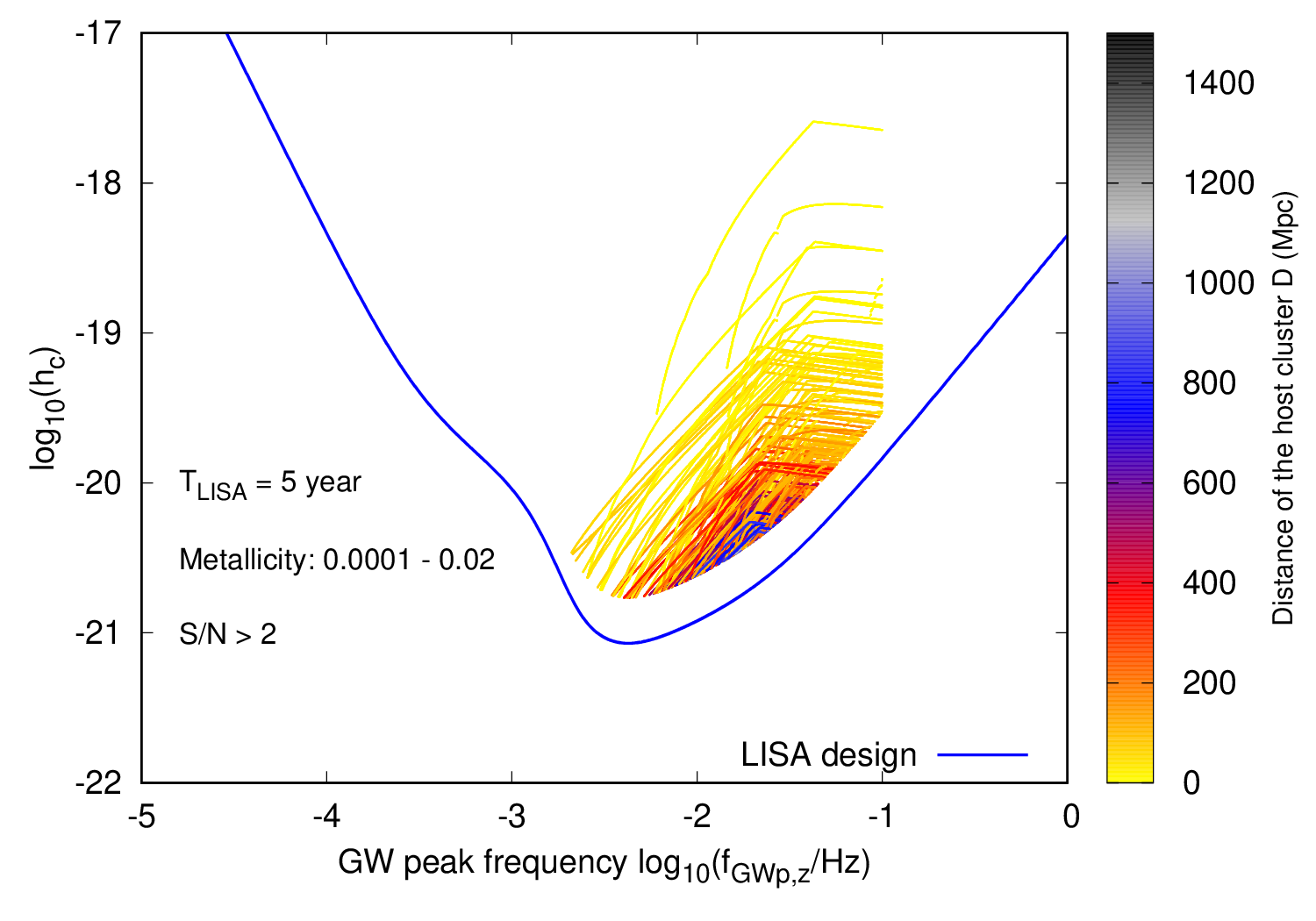
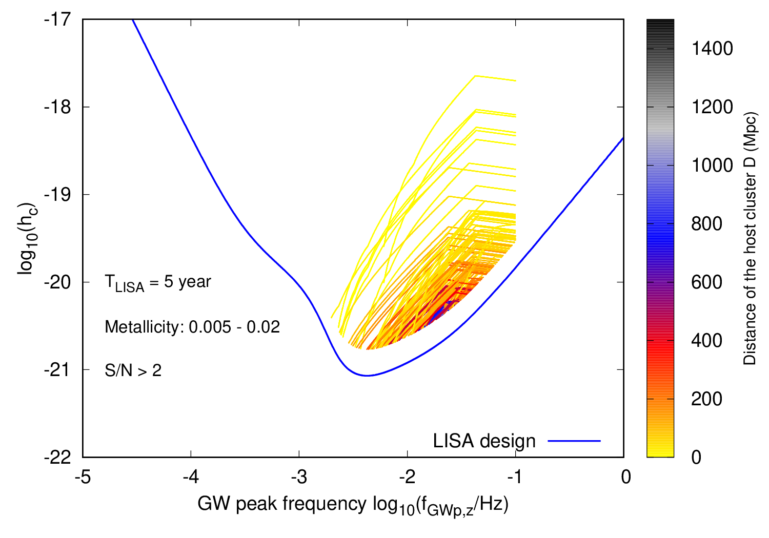
Figure 1: BBH inspirals at the present cosmic age (within $t_{\rm Hubble}\pm 0.1$ Gyr), over the characteristic LISA frequency range ($10^{-3}{\rm~{}Hz}-10^{-1}{\rm~{}Hz}$), from a representative sample of the Local Universe ($D\leq 1500$ Mpc) as constructed with the computed model clusters (Sec. II). The inspirals are shown (thin lines) in the plane of redshifted GW peak frequency in the detector frame, $f_{\rm GWp,z}$, versus GW characteristic strain at this frequency, $h_{\rm c}$, for those systems which have S/N $\geq 2$ w.r.t. LISA’s design sensitivity curve (thick, blue line). The $h_{\rm c}-f_{\rm GWp,z}$ tracks are colour-coded (colour bar) according to the distance of the BBH’s host cluster. The left and right panels show the outcomes when the metallicity range of the model clusters in the Local-Universe sample is taken to be $0.0001-0.02$ and $0.005-0.02$, respectively. A LISA mission lifetime of $T_{\rm LISA}=5{\rm~{}yr}$ is assumed.

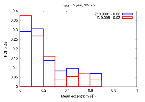
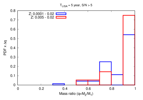
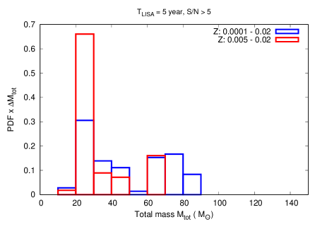
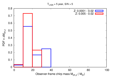
Figure 2: Properties of LISA BBH sources, with S/N $>5$, at the present cosmic age from a representative Local Universe constructed with the computed model clusters (Sec. II). The top left, top right, bottom left, and bottom right panels respectively show the probability distributions of the sources’ mean eccentricity (Sec. III), $\overline{e}$, mass ratio, $q$, total mass, $M_{\rm tot}$, and detector-frame (redshifted) chirp mass, $M_{\rm ch,z}$. On each panel, the blue- and red-lined histograms correspond to the cluster metallicity ranges $0.0001-0.02$ and $0.005-0.02$, respectively. A LISA mission lifetime of $T_{\rm LISA}=5{\rm~{}yr}$ is assumed.

If the redshift at the cluster’s distance is $z_{\rm D}$ then the detector-frame (redshifted) peak GW frequency, its chirp, and the chirp mass are given by

$$\left.\begin{aligned} f_{\rm GWp,z}=&\frac{f_{\rm GWp}}{(1+z_{\rm D})}\\ \dot{f}_{\rm GWp,z}=&\frac{\dot{f}_{\rm GWp}}{(1+z_{\rm D})^{2}}\\ M_{\rm ch,z}=&M_{\rm ch}(1+z_{\rm D})\end{aligned}\right\}$$ (15)

The detector-frame chirp mass can be obtained by rewriting Eqn. 8 in terms of $f_{\rm GWp,z}$, and $\dot{f}_{\rm GWp,z}$.

In this work, a GW source is considered visible by LISA if, (i), its GW frequency lies within a relatively narrow range, $10^{-3}{\rm~{}Hz}\leq f_{\rm GWp,z}\leq 10^{-1}{\rm~{}Hz}$, around the instrument’s noise floor minimum or ‘bucket frequency’ (at $\sim 10^{-2}{\rm~{}Hz}$; Amaro-Seoane et al. (2017); Robson et al. (2019)). At the same time, (ii), a LISA-visible source should at most be moderately eccentric, $e\leq 0.7$ (Nishizawa et al., 2016, 2017; Chen and Amaro-Seoane, 2017), so that it is not ‘bursty’. Note that a source is effectively lesser detectable the slower the evolution of $f_{\rm GWp,z}$ ($f_{\rm GWp}$) is over the LISA mission lifetime, $T_{\rm LISA}$. This is taken into account by multiplying a reduction factor to the GW characteristic strain as given by Eqn. 10:

$$h_{c}=\kappa\times\tilde{h}_{c},$$ (16)

where (Sesana et al., 2005; Willems et al., 2007; Kremer et al., 2019)

$$\kappa=\min\left(\sqrt{\frac{\dot{f}_{\rm GWp,z}}{f_{\rm GWp,z}}T_{\rm LISA}},{\rm~{}~{}}1\right).$$ (17)

Here, mission lifetimes of $T_{\rm LISA}=5$ year (planned) and 10 year (optimistic) are considered.

Finally, (iii), $h_{c}$ should exceed a signal to noise ratio (hereafter S/N) threshold for visibility. In this work, LISA sources with S/N $>0$, $\geq 2$, $\geq 5$, and $\geq 10$ are considered; the source count with S/N $>0$ implies the intrinsic count. The analytical LISA design sensitivity curve (or noise floor) (Robson et al., 2019), which closely reproduces the instrument’s published design sensitivity curve (Amaro-Seoane et al., 2017) over the visibility frequency-window considered here, is utilized in determining S/N for the LISA sources form the sample Local Universe. In terms of characteristic strain, this sensitivity curve as a function of (detector-frame) GW frequency, $f$, is given by

$$\left.\begin{aligned} h_{\mathcal{N}}(f)=&f^{1/2}\sqrt{S_{\mathcal{N}}(f)+S_{\rm g}(f)}\\ S_{\mathcal{N}}(f)=&\frac{P_{\mathcal{N}}(f)}{\mathcal{R}(f)}.\end{aligned}\right\}$$ (18)

Here, $P_{\mathcal{N}}(f)$ is the power spectral density of the (LISA) instrument noise and $\mathcal{R}(f)$ is the sky- and polarization-averaged, two-channel (since LISA has two independent data channels) signal response function. The added $S_{\rm g}(f)$ is the power spectral density (divided by two due to the two-channel instrument) of the confusion noise due to unresolved Galactic binaries.

With the analytic fit to the response function, as given by

$$\mathcal{R}(f)=\frac{3}{10}\frac{1}{(1+0.6(f/f_{\ast})^{2})},$$ (19)

$$S_{\mathcal{N}}(f)= \frac{10}{3L^{2}}\left(P_{\rm OMS}(f)+2(1+\cos^{2}(f/f_{\ast}))\frac{P_{\rm acc}(f)}{(2\pi f)^{4}}\right)$$ (20)

$$\times\left(1+\frac{6}{10}\left(\frac{f}{f_{\ast}}\right)^{2}\right).$$

The functions $P_{\rm OMS}(f)$ (single-link optical metrology noise) and $P_{\rm acc}(f)$ (single test mass acceleration noise) are given by (as in “LISA Strain Curves” document LISA-LCST-SGS-TN-001)

$$\left.\begin{aligned} P_{\rm OMS}(f)=&(1.5\times 10^{-11}{\rm~{}m})^{2}\left(1+\left(\frac{\rm 2~{}mHz}{f}\right)^{4}\right){\rm Hz}^{-1}\\ P_{\rm acc}(f)=&(3\times 10^{-15}{\rm~{}m~{}s^{-2}})^{2}\left(1+\left(\frac{\rm 0.4~{}mHz}{f}\right)^{2}\right)\\ &\times\left(1+\left(\frac{f}{\rm 8~{}mHz}\right)^{4}\right){\rm Hz}^{-1}\end{aligned}\right\}$$ (21)

and the instrument constants are $L=2.5{\rm~{}Gm}$ (LISA arm length) and $f_{\ast}=19.09{\rm~{}mHz}$. The Galactic confusion noise is given by the fitting function

$$S_{\rm g}(f)=Af^{-7/3}e^{-f^{\alpha}+\beta f\sin(Kf)}\left[1+\tanh(\gamma(f_{k}-f))\right]{\rm Hz}^{-1}$$ (22)

with $A=9\times 10^{-45}$, $\alpha=0.138$, $\beta=-221$, $K=521$, $\gamma=1680$, and $f_{k}=0.00113$. See (Robson et al., 2019) and references therein for the derivations of Eqns. 19, 20, 21, and 22.

The resulting LISA design sensitivity curve is shown in the panels of Fig. 1 (thick, blue line). Note that $f_{k}$ and $\gamma$ in Eqn. 22 vary moderately with observation time resulting in an increasingly steeper drop-off of $S_{\rm g}(f)$. Here, for simplicity, the 4-year values of all the parameters in Eqn. 22, as stated above (Robson et al., 2019), are used. Note that over most of the LISA detection frequency range, $S_{\mathcal{N}}$ is the dominant noise except that $S_{\rm g}$ causes the mild ‘hump’ feature in the total sensitivity curve, as seen in Fig. 1.

In this work, for simplicity, S/N is preliminarily taken to be (recalling Eqn. 16)

$$\left(\frac{\rm S}{\rm N}\right)\approx\frac{h_{c}(f_{\rm GWp})}{h_{\mathcal{N}}(f_{\rm GWp,z})}=\frac{\kappa(f_{\rm GWp,z})\tilde{h}_{c}(f_{\rm GWp})}{h_{\mathcal{N}}(f_{\rm GWp,z})}$$ (23)

$[f_{\rm GWp}=(1+z_{\rm D})f_{\rm GWp,z}]$ which is evaluated along an in-spiralling orbit using Eqns. 5, 6, 10, 17, and 18-22 (in the practical computations a lookup table for the LISA design noise strains, generated using Eqns. 20-22, is utilized). A more elaborate expression of S/N is given by summing over all harmonics (O’Leary et al., 2009):

$$\left(\frac{\rm S}{\rm N}\right)=\sqrt{\sum_{n=1}^{\infty}\int_{f_{n,0}}^{f_{n,{T_{\rm LISA}}}}\left[\frac{\tilde{h}_{c,n}(f^{\prime}_{n})}{h_{\mathcal{N}}(f_{n})}\right]^{2}d\ln f_{n}}$$ (24)

$[f^{\prime}_{n}=(1+z_{\rm D})f_{n}]$ . Here, $f_{n}$ is the detector-frame GW frequency of the $n$th harmonic (see above), and ($f_{n,0}$, $f_{n,{T_{\rm LISA}}}$) is the GW frequency of this harmonic at the (start, end) of LISA observation at time ($0$, $T_{\rm LISA}$). $\tilde{h}_{c,n}(f^{\prime}_{n})$ is the GW characteristic strain corresponding to the $n$th harmonic as given by Eqn. 14.

Since the majority of the LISA-visible binaries have mild eccentricity (due to condition ii and also GR orbital evolution; see below), the GW power is sharply peaked at the peak GW frequency $f_{\rm GWp}$ ($f_{\rm GWp,z}$) (Peters and Mathews, 1963) which corresponds to the harmonic $n_{p}\lesssim 10$ (see above). In that case, Eqn. 24 becomes, to the leading order,

$$\left(\frac{\rm S}{\rm N}\right)\approx \sqrt{\int_{0}^{T_{\rm LISA}}\left[\frac{\tilde{h}_{c}(f_{\rm GWp})}{h_{\mathcal{N}}(f_{\rm GWp,z})}\right]^{2}\frac{\dot{f}_{\rm GWp,z}}{f_{\rm GWp,z}}dt}$$ (25)

$$\approx \sqrt{\left[\frac{\tilde{h}_{c}(f_{\rm GWp})}{h_{\mathcal{N}}(f_{\rm GWp,z})}\right]^{2}\frac{\dot{f}_{\rm GWp,z}}{f_{\rm GWp,z}}T_{\rm LISA}}$$

$$= \frac{\kappa(f_{\rm GWp,z})\tilde{h}_{c}(f_{\rm GWp})}{h_{\mathcal{N}}(f_{\rm GWp,z})}$$

$[f_{\rm GWp}=(1+z_{\rm D})f_{\rm GWp,z}]$ where the last equality is due to Eqn. 17. In the second approximate relation in Eqn. 25, the integrand, to its leading order, is taken to remain constant at its mean value over $T_{\rm LISA}$ since its variation over $T_{\rm LISA}$ is typically small ($\kappa<1$ for most sources here; see Fig. 3 and the associated discussions below). Therefore, the approximate S/N, as given by Eqn. 23, serves as a good approximation for and captures the essential properties of the full definition, for the LISA sources in this work .

The squared value of $\kappa$ (Eqn. 17) at the minimum $f_{\rm GWp,z}$ for which the visibility conditions (i), (ii), and (iii) are simultaneously satisfied (i.e., at the source’s ‘entry’ to the visibility band) is referred to in this work as the ‘transience’, $\kappa_{1}$, of the LISA source. $\kappa_{1}\leq 1$ is a measure of how transient the source is over the LISA lifetime: the larger is $\kappa_{1}$ the more will the source’s $f_{\rm GWp,z}$ and other properties evolve (due to its PN inspiral) over the mission lifetime. $\kappa_{1}=1$ implies that the source evolves in a timescale $\leq T_{\rm LISA}$.

In this study, the standard ($\Lambda$CDM) cosmological framework is adopted (Wright, 2006) with the cosmological constants from the latest Planck results ($H_{0}=67.4{\rm~{}km~{}s}^{-1}{\rm~{}Mpc}^{-1}$, $\Omega_{\rm~{}m}=0.315$, and flat Universe for which $t_{\rm Hubble}=13.79{\rm~{}Gyr}$) (Planck Collaboration et al., 2018).

III LISA sources from young massive and open stellar clusters

Fig. 1 shows examples of BBH inspirals in the LISA band from a sample Local Universe that are ‘detected’ (i.e., satisfy the visibility conditions i-iii) at the present cosmic age with S/N $\geq 2$ (i.e., at $\left\lvert t_{\rm obs}-t_{\rm Hubble}\right\rvert\leq\Delta t_{\rm obs}\left[=0.1{\rm~{}Gyr}\right]$), using the method described in Sec. II.2. Fig. 1 shows the detected inspirals (as dictated by Eqns. 6, 10, and 17) in the $h_{c}-f_{\rm GWp,z}$ plane for the $Z$ ranges 0.0001-0.02 and 0.005-0.02 and for $T_{\rm LISA}=5$ year (see Table 1). The design sensitivity curve of LISA (Robson et al., 2019) is shown in the same plane (the thick, blue line). In the following, unless otherwise stated, present-day (or present-cosmic-age) LISA sources will imply only those that are detected in the above sense. Note that depending on the strength of a particular source (given its distance, mass, and orbital properties), it may be detectable over only a sub-window within the full detection frequency range $10^{-3}{\rm~{}Hz}-10^{-1}{\rm~{}Hz}$ (see Fig. 1).

If for the $T_{\rm LISA}$ mission time the total number of present-day LISA sources with S/N $\geq s$, from a sample Local Universe comprising ${\rm N}_{\rm samp}$ clusters, is ${\rm N}_{>s}$ then the estimated number of present-day LISA sources within a $T_{\rm LISA}$ window, ${\mathcal{N}}_{>s}$, is

$${\mathcal{N}}_{>s}=\frac{4}{3}\pi D_{\rm max}^{3}\rho_{\rm cl}\frac{{\rm N}_{>s}}{{\rm N}_{\rm samp}}\frac{T_{\rm LISA}}{2\Delta t_{\rm obs}},$$ (26)

where $\rho_{\rm cl}$ is the present-day volume density of young clusters in the Local Universe. Eqn. 26 can be rewritten as (for the assumed $D_{\rm max}=1500{\rm~{}Mpc}$; see Sec. II.2),

$$\frac{{\mathcal{N}}_{>s}}{\rho_{\rm cl}/{\rm~{}Mpc}^{-3}}=7.069\frac{{\rm N}_{>s}}{{\rm N}_{\rm samp}}\frac{(T_{\rm LISA}/{\rm yr})}{(\Delta t_{\rm obs}/{\rm Gyr})}.$$ (27)

Table 1 shows the ${\rm N}_{>s}$ and ${\mathcal{N}}_{>s}/\rho_{\rm cl}$ values for $s=2$, 5, and 10 for four Local-Universe samples with $Z$-ranges $0.0001-0.02$ and $0.005-0.02$ and $T_{\rm LISA}=5{\rm~{}yr}$ and 10 yr. Also shown are the intrinsic source counts, ${\rm N}_{0}$ and ${\mathcal{N}}_{0}/\rho_{\rm cl}$, corresponding to S/N $>0$. For each Local Universe, ${\rm N}_{\rm samp}\approx 2.3\times 10^{4}$. By taking half of this ${\rm N}_{\rm samp}$, it is found that all the source counts also become nearly half, implying that such ${\rm N}_{\rm samp}$ yields statistically convergent counts.

Fig. 2 shows the probability distributions (probability density function; hereafter PDF) of the properties of LISA BBH sources at the present cosmic age, that have S/N $>5$, as compiled from Local-Universe samples with $Z$-ranges $0.0001-0.02$ (blue-lined histogram) and $0.005-0.02$ (red-lined histogram). All the distributions in Fig. 2 correspond to $T_{\rm LISA}=5$ year. The top-left panel shows the PDF of the ‘mean eccentricity’, $\overline{e}$, over the detected GW frequency window. $\overline{e}$ represents the most likely eccentricity of the BBH when its GW signal is observed by the detector and is measured, in this study, by the expression

$$\overline{e}=\frac{(2-\kappa_{1})e_{1}+\kappa_{1}e_{2}}{2}.$$ (28)

Here $\kappa_{1}$ is the transience of the GW source as defined in Sec. II.2. When $\kappa_{1}\rightarrow 0$ (the source is nearly invariant over $T_{\rm LISA}$), $\overline{e}\rightarrow e_{1}$, the eccentricity of the binary at the minimum $f_{\rm GWp,z}$ satisfying the visibility conditions. When $\kappa_{1}=1$ (the source is variable over timescales $\leq T_{\rm LISA}$), $\overline{e}=(e_{1}+e_{2})/2$, midway between the eccentricities, $e_{1}$ and $e_{2}$ respectively ($e_{1}>e_{2}$), at the minimum and maximum $f_{\rm GWp,z}$ satisfying the visibility conditions (see Fig. 1).

The cutoff of the $\overline{e}$ distribution at $\overline{e}=0.7$ is simply due to the adopted criterion $e\leq 0.7$ for visibility by LISA (Sec. II.2). Despite the fact that the BBHs’ PN inspirals typically start with a high $e$, the majority of those with $e\leq 0.7$ are already well circularized within the adopted ‘bucket’ frequency range of $10^{-3}{\rm~{}Hz}-10^{-1}{\rm~{}Hz}$ (see Fig. 10 of Banerjee (2020); see also Banerjee (2018a)). This causes the PDF to increase with decreasing $\overline{e}$ (top-left panel of Fig. 2). As typical for dynamically-assembled BBH inspirals (Di Carlo et al., 2019; Banerjee, 2020), which is the case for the vast majority of inspirals from the present models, the distribution of the mass-ratio, $q\equiv{\rm M}_{2}/{\rm M}_{1}$ (${\rm M}_{1}\geq{\rm M}_{2}$), of the LISA-visible BBHs is strongly biased towards unity (Fig. 2, top-right panel). However, sources as asymmetric as $q<0.4$ is possible for a Local Universe extending to the metal-poorest environments.

The distribution of the total mass, $M_{\rm tot}$, of the LISA BBH sources is bimodal (Fig. 2, bottom-left panel). The lower mass peak (spanning over $20M_{\odot}-40M_{\odot}$) is due to the ambience of lower mass BBH inspirals over the $\lesssim 5$ Gyr delay times considered here (Sec. II.2); see Fig. 9 of (Banerjee, 2020). The higher mass peak, beyond $60M_{\odot}$, appears since despite the relative rarity of such massive BBH inspirals they are the brightest GW sources (with highest $\tilde{h}_{c}$ and $\kappa$). Note that this bimodal feature appears irrespective of the metallicity range of the Local Universe. The feature is also mildly present in the PDF of the detector-frame chirp mass, $M_{\rm ch,z}$, of the LISA BBH sources (Fig. 2, bottom-right panel).

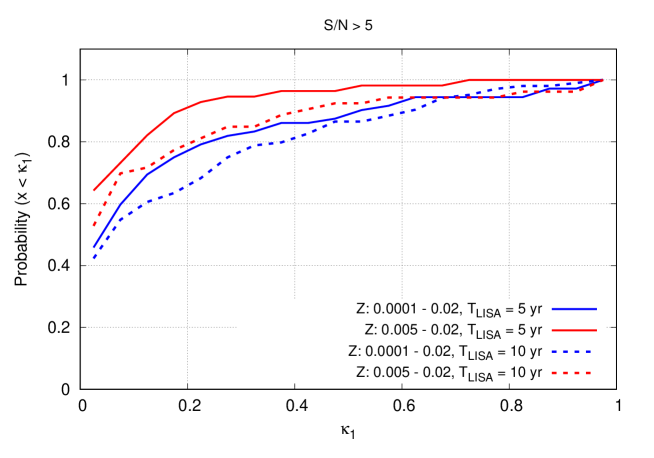
Figure 3: Cumulative probability distribution of the transience, $\kappa_{1}$ (Eqn. 17, Sec. II.2), of LISA BBH sources, with S/N $>5$, at the present cosmic age from a representative Local Universe constructed with the computed model clusters (Sec. II). The distributions are shown for both metallicity ranges $0.0001-0.02$ and $0.005-0.02$ and for $T_{\rm LISA}=5$ and 10 year LISA mission lifetimes, as indicated in the legend.

Fig. 3 shows the cumulative probability distribution of the transience, $\kappa_{1}$ (Sec. II.2), of the present-day LISA BBH sources that have S/N $>5$, as compiled from the Local-Universe samples considered here. Shown are the cumulative PDFs for both metallicity ranges $0.0001-0.02$ (blue lines) and $0.005-0.02$ (red lines) and for $T_{\rm LISA}=5$ year (solid lines) and 10 year (dashed lines). A LISA source would reach merger, i.e., exit the LISA band and become visible in the LIGO-Virgo band, within twice the LISA mission time if $\kappa_{1}\geq 0.5$. According to Fig. 3, with S/N $>5$ and $T_{\rm LISA}=5$ year, the fraction of BBHs exhibiting such ‘LISA-LIGO’ visibility (Sesana, 2016) is $\approx 15$% ($\approx 5$%) for the $0.0001\leq Z\leq 0.02$ ($0.005\leq Z\leq 0.02$) Local Universe. With S/N $>5$ and $T_{\rm LISA}=10$ year, the fraction is $\approx 15$% ($\approx 10$%) for $0.0001\leq Z\leq 0.02$ ($0.005\leq Z\leq 0.02$).

With an estimate of the local volume density of YMCs and OCs, $\rho_{\rm cl}$, the values of ${\mathcal{N}}_{>s}/\rho_{\rm cl}$ in Table 1 can be utilized to estimate the present-day LISA BBH source count. Here a preliminary estimate of $\rho_{\rm cl}$ is used, which is based on the observed local density of GCs of $\rho_{\rm GC}\approx 2.6{\rm~{}Mpc}^{-3}$ (van den Bergh, 1995; Portegies Zwart and McMillan, 2000) (taking $h\equiv H_{0}/[100{\rm~{}km~{}s}^{-1}]=0.674$). Due to the observed power-law birth mass function of clusters with index $\approx-2$ (Lada and Lada, 2003; Gieles et al., 2006a, b; Larsen, 2009) alone, YMCs and OCs of the mass range considered here ($10^{4}M_{\odot}-10^{5}M_{\odot}$) would be $\approx 20$ times more numerous than GCs (Banerjee, 2018a), resulting in $\rho_{\rm cl}\approx 52{\rm~{}Mpc}^{-3}$. The number of LISA BBH sources, for $T_{\rm LISA}=5$ year, would accordingly be ${\mathcal{N}}_{>2}\approx 174$, ${\mathcal{N}}_{>5}\approx 56$, ${\mathcal{N}}_{>10}\approx 31$ (${\mathcal{N}}_{>2}\approx 107$, ${\mathcal{N}}_{>5}\approx 44$, ${\mathcal{N}}_{>10}\approx 23$) from the Local Universe with $0.0001\leq Z\leq 0.02$ ($0.005\leq Z\leq 0.02$). For $T_{\rm LISA}=10$ year, ${\mathcal{N}}_{>2}\approx 483$, ${\mathcal{N}}_{>5}\approx 164$, ${\mathcal{N}}_{>10}\approx 71$ (${\mathcal{N}}_{>2}\approx 252$, ${\mathcal{N}}_{>5}\approx 85$, ${\mathcal{N}}_{>10}\approx 48$) for $0.0001\leq Z\leq 0.02$ ($0.005\leq Z\leq 0.02$). For $T_{\rm LISA}=5$ year, the intrinsic count for LISA-visible BBHs is ${\mathcal{N}}_{0}\approx 1039$ (${\mathcal{N}}_{0}\approx 727$) from the Local Universe with $0.0001\leq Z\leq 0.02$ ($0.005\leq Z\leq 0.02$). For $T_{\rm LISA}=10$ year, ${\mathcal{N}}_{0}\approx 2008$ (${\mathcal{N}}_{0}\approx 1484$) for $0.0001\leq Z\leq 0.02$ ($0.005\leq Z\leq 0.02$).

IV Summary and discussions

This study, for the first time, attempts to assess the potential contribution of YMCs and OCs, within the Local Universe, in assembling stellar-mass BBHs that are detectable by LISA as per the instrument’s proposed design. To that end, a suite of state-of-the-art, direct, PN N-body evolutionary model clusters, incorporating up-to-date stellar-evolutionary and remnant-formation models and observationally-consistent structural properties and stellar ingredients (Banerjee, 2020), is utilized (Sec. II.1). The model set allows to explore the cluster mass range of $10^{4}M_{\odot}-10^{5}M_{\odot}$ representing the regime where clusters form as YMCs, over the cosmic SFH, and evolve in long term to become moderately-massive, $\sim{\rm~{}Gyr}$-old OCs. In this study, model clusters up to $\approx 5$ Gyr age (formation redshift $\leq 0.5$) are explored, as typical for intermediate-aged OCs. The BBH inspirals from them, that would be present at the current cosmic epoch in LISA’s most sensitive GW frequency range of $10^{-3}{\rm~{}Hz}-10^{-1}{\rm~{}Hz}$ with eccentricity $<0.7$ and exceeding an S/N threshold (Fig. 1), are tracked (Sec. II.2). For this purpose, samples of Local Universe, comprising $\sim 10^{4}$ clusters (Table 1) and having a LISA visibility limit of 1500 Mpc, are constructed out of the evolutionary cluster models, following the observed cluster birth mass function and SFH and adopting the standard cosmological framework (Sec. II.2). A sample Local Universe comprises either the full metallicity range of the cluster models, $0.0001\leq Z\leq 0.02$ (most of which have $Z\geq 0.001$), implying that the Local Volume well includes LMC-like or sub-LMC metal-poor environments or only the $0.005\leq Z\leq 0.02$ models implying that the Local Volume is made predominantly of metal-rich environments (Table 1).

A drawback of the present approach is that a cluster’s metallicity is completely decoupled from its formation epoch according to the cosmic SFH. However, this is not critical since only recent formation redshifts of $z_{\rm f}\leq 0.5$ are considered. How ambient are metal-poor environments in the Local Universe is still largely an open question (Hsyu et al., 2018; Izotov et al., 2018). Rather, the two $Z$ ranges considered here enable exploring the impact of metallicity on LISA source counts and properties. Indeed, the Local Universe including the metal-poor clusters typically yields larger, by up to a factor of two, present-day LISA source counts (Table 1). This is due to the fact that low-$Z$ clusters yield more massive BBH inspirals (since low-$Z$ stellar progenitors produce more massive BHs Belczynski et al. (2010); Banerjee et al. (2020)) so that the present-day LISA BBHs are biased towards higher masses (Fig. 2, bottom panels), which are also generally brighter GW sources. In a forthcoming study, metallicity-dependent SFH (e.g., Madau and Fragos (2017); Chruslinska and Nelemans (2019)) will be applied in such an exercise.

For both metallicity regimes, the distribution of total mass, $M_{\rm tot}$, of the present-day LISA BBHs exhibits a bimodal feature (Fig. 2, bottom-left panel; Sec. III). For both cases, the present-day LISA BBH sources are predominantly of similar component masses (mass ratio $q\approx 1$) although dissimilar-mass sources of $q<0.4$ are possible from the metal-poorer Local Universe (Fig. 2, top-right panel). For both type of Local Universe, the present-day LISA BBH sources are generally eccentric ($e<0.7$), although they are biased towards being circular (Fig. 2, top-left panel; Sec. III).

Stellar-mass LISA BBH sources are persistent, with the source properties varying mildly (as given by their transience, $\kappa_{1}$; Sec. II.2) over the LISA mission lifetime, $T_{\rm LISA}$, for the majority of them. However, a small fraction of them would still exhibit significant evolution as they undergo PN inspiral. For the metal-poorer Local Universe, $\approx 15$% of the present-day LISA BBHs with S/N $>5$ would show up in the LIGO-Virgo frequency band within twice the mission lifetime and $<5$% of the sources would do so within the mission time, for $T_{\rm LISA}=5$ year or 10 year (Fig. 3; Sec. III). For the metal-richer Local Universe, the former fraction is $<10$%.

Table 1 shows the estimated number of present-day LISA BBH sources, ${\mathcal{N}}_{>s}$, with S/N thresholds $s=2$, 5, and 10, for both metallicity regimes and for 5 year and 10 year mission lifetimes. The entries are scaled w.r.t. the present-day volume density, $\rho_{\rm cl}$, of YMCs and OCs in the Local Universe (see Eqn. 27). Since such clusters continue to form and evolve with the cosmic evolution of star formation (Madau and Dickinson, 2014), $\rho_{\rm cl}$ depends on the fraction of stars forming in bound clusters and the fraction of such clusters surviving the violent birth environment and conditions (Marks and Kroupa, 2012; Marks et al., 2012; Longmore et al., 2014; Krumholz et al., 2014; Banerjee and Kroupa, 2018; Renaud, 2018), all of which, and hence $\rho_{\rm cl}$, are poorly constrained to date. By scaling the observed volume density of GCs based on observed cluster mass function, it can be inferred that YMCs and OCs of $\lesssim 5$ Gyr age in the metal-poorer Local Universe would provide $\approx 56$ ($\approx 164$) LISA BBH sources with S/N $>5$, for 5 year (10 year) mission time (Table 1; Sec. III). For the metal-richer Local Universe, the corresponding source counts are $\approx 44$ ($\approx 85$). Therefore, YMCs and OCs would yield LISA-visible BBHs in about an order of magnitude larger numbers than those from GCs (Kremer et al., 2019). Intrinsically, there would be $\approx 1000$ (700) present-day, LISA-visible BBHs from YMCs and OCs in the metal-poorer (metal-richer) Local Universe, for $T_{\rm LISA}=5$ year (Table 1; Sec. III). For $T_{\rm LISA}=10$ year, the intrinsic counts nearly double.

Note that the above estimates of present-day LISA sources still represent lower limits. The counts can easily be a few factors higher if the borderline between intermediate-aged OCs and GCs is set at a higher mass (currently, it is $10^{5}M_{\odot}$ Banerjee (2018a)). Also, considering clusters formed at higher redshifts would add to both the present-day source counts from a sample Local Universe and the present-day local density of YMCs and OCs, which would also lead to a few factors boost in the source counts.

LISA BBH sources in young clusters has been addressed also in other recent studies (Rastello et al., 2019; Di Carlo et al., 2019). The eccentricity distribution of LISA BBH sources, as obtained here, qualitatively agrees with the trend of the same presented in (Di Carlo et al., 2019). But unlike from these authors, the LISA BBH sources here extend to much higher eccentricities, all the way up to 0.7 (Fig. 2, top-left panel). Note, although, that these authors provide the eccentricity distribution corresponding to $f_{\rm K}=10^{-2}$ Hz whereas here the most likely eccentricity over $10^{-3}{\rm~{}Hz}\leq f_{\rm GWp,z}\leq 10^{-1}{\rm~{}Hz}$ (Eqn. 28) is considered. Furthermore, in Di Carlo et al. (2019), nearly all in-spiralling systems (that merge within a Hubble time) are dynamically ejected from the clusters whereas here the inspirals take place either inside the clusters or after getting ejected, the former type being dominant (Banerjee, 2017; Anagnostou et al., 2020). Finally, the present work considers clusters of much higher mass (by a few to 100 times) and much longer evolutionary times than those in (Di Carlo et al., 2019), yielding BBH inspirals of much broader orbital morphology. The range and the trend of the eccentricity distribution of LISA BBHs obtained here are qualitatively similar to those for in-cluster inspirals from computed GC models (Kremer et al., 2019), which are a few to 10 times more massive than the present models but incorporate similar physics ingredients.

In the near future, this line of study will be extended to incorporate cosmic metallicity evolution and SFH up to high redshifts. The same methodology can be applied to obtain LIGO-Virgo compact binary merger rates from YMCs and OCs, which study is underway (see, e.g., Santoliquido et al. (2020) for an alternative approach). The present set of computed model clusters is being extended in mass and density.