In situ exo-planet transit lightcurve modelling with the Chroma+ suite

Abstract

We have added to the Chroma+ suite of stellar atmosphere and spectrum modelling codes the ability to synthesize the exo-planet transit lightcurve for planets of arbitrary size up to 10% of the host stellar radius, and arbitrary planetary and stellar mass and orbital radius (thus determining orbital velocity) and arbitrary orbital inclination. The lightcurves are computed in situ, integrated with the radiative transfer solution for the radiation field emerging from the stellar surface, and there is no limb-darkening parameterization. The lightcurves are computed for the Johnson-Bessel photometric system $UBVRIHJK$. We describe our method of computing the transit path, and the reduction in flux caused by occultation, and compare our lightcurve to an analytic solution with a four-parameter limb-darkening parameterization for the case of an edge-on transit of the Sun by Earth. This capability has been added to all ports and variations, including the Python port, ChromaStarPy, and the version that interpolates among the fully line-blanketed ATLAS9 surface intensity distributions, ChromaStarAtlas. All codes may be accessed at www.ap.smu.ca/OpenStars and at GitHub (github.com/sevenian3).

1 Introduction

Transit lightcurve analysis has become an important tool in determining the properties of exo-planets and of their orbital parameters, and of the host star. They pose an interesting inverse-problem and much effort has gone into extracting information about the system from the detected lightcurve, and most of these methods rely in one way or another on a parameterization of the host star’s limb-darkening profile. The limb-darkening coefficients (LDCs) that parameterize a limb-darkening law are wavelength- and band-pass- sensitive and must be determined for each photometric system, and for each set of host star parameters. Moreover, limb-darkening laws are necessarily an approximation to the real variation of specific intensity with angle of emergence from the host star’s surface, $I_{\lambda}(\cos\theta)$.

We have implemented a complementary forward-modelling approach by incorporating the calculation of transit lightcurves, $F_{\rm band}(t)$, in the Chroma+ suite of stellar atmosphere and spectrum modelling codes for the Johnson-Bessel $U_{\rm x}BVRI$ (Johnson et al., 1966) and Johnson $HJK$ (Johnson, 1965) photometric systems. Our procedure computes $F_{\rm band}(t)$ in situ because it is integrated with the radiative transfer solution for the emergent surface intensity $I_{\lambda}(\tau=0,\cos\theta)$ for the atmospheric structure, where $\tau$ is any vertical optical depth scale increasing inward. Therefore, there is no limb-darkening parameterization. This approach was also taken by Neilson et al. (2017) to evaluate the accuracy of LDC-based lightcurve analysis using $I_{\lambda}(\tau=0,\cos\theta)$ distributions computed with the plane-parallel and spherical versions of the ATLAS9 (Castelli & Kurucz, 2006) stellar atmosphere and spectrum modelling suite. Our simulated $F_{\rm band}(t)$ curves may be used to evaluate the accuracy of LDC-based inverse methods, as well as for the forward modelling of observed $F_{\rm band}(t)$ signals with a grid that explores host-star, planetary, orbital parameter, and orientation space.

We have added $F_{\rm band}(t)$ calculation to the entire Chroma+ suite, including the Python implementation ChromaStarPy (CSPy, Short, Bayer & Burns (2018)), which provides for fast modelling and analysis in a Python IDE, and ChromaStarAtlas (Short & Bayer, 2018), in which the $I_{\lambda}(\tau=0,\cos\theta)$ distribution being occulted is the fully line blanketed distribution interpolated with the public ATLAS9 $I_{\lambda}(\tau=0,\cos\theta)$ distributions of Castelli & Kurucz (2006).

2 Method

The radiative transfer procedure of the Chroma+ suite computes the emergent monochromatic surface specific intensity distribution, $I_{\lambda}(\tau=0,\cos\theta)$, for a set of direction angles, $\{\cos\theta\}$, with respect to the local stellar surface normal that have a Gauss-Legendre distribution in the $\cos\theta$ range $[1,0]$, over a wide range of $\lambda$ from the UV to the IR with equal $\log\lambda$ spacing supplemented with ad hoc additional $\lambda$ points for spectral lines. This is the $I_{\lambda}(\tau=0,\cos\theta)$ distribution that is occulted as an exo-planet transits the host star as seen by an observer on Earth.

2.1 Assumptions

We adopt the following simplifying assumptions for the planetary system: 1) The exo-planet orbital radius, $R_{\rm orb}$, is large enough compared to the stellar radius, $R$, that the transit path is a chord in the plane of the sky, 2) The exo-planet’s orbit is Copernican so that, along with assumption 1), the component of orbital velocity, $v_{\rm orb}$, in the plane-of-the-sky is constant during transit and is equal to $v_{\rm orb}$, 3) The planet’s radius, $r$, is small enough to occult only one $\Delta\cos\theta$ substellar-centric annulus in the discretization in the plane of the sky of the host stellar atmosphere radiation field at any time $t$, 4) Only transits in which the entire projected area of the planetary disk is occulting at mid-transit are of interest, 5) The planet has a specific intensity of zero, 6) The distance to the system, $d$, is large compared to $R_{\rm orb}$ so that the occulted flux may be calculated at the stellar surface, and so that, along with assumptions 1) and 2), the transit velocity is equal to $v_{\rm orb}$. Assumption 3) is the ”small planet approximation” investigated by Mandel & Agol (2002) and corresponds to $r/R\lesssim 0.1$. Assumption 4) is consistent with Assumption 3), and disregards grazing transits, which are less detectable.

2.1.1 Inputs

In addition to the host stellar parameters required for static $1D$ horizontally homogenous plane-parallel modelling of the host stellar atmosphere ($T_{\rm eff},\log g,[{{\rm A}\over{\rm H}}],\xi_{\rm T}$), the procedure also requires the radius of the exo-planet orbit, $R_{\rm orb}$, the radius of the exo-planet, $r$, and the inclination of the planetary orbital axis with respect to the line-of-sight, $i$. As part of the established Chroma+ modelling procedure, the user also specifies an input stellar mass, $M$, which the Chroma+ codes combine with the input $\log g$ value to compute the host star’s radius, $R$. We assume that the system is Keplerian ($m_{\rm planet}<<M$) so that $v_{\rm orb}$ is found from $v^{2}_{\rm orb}=GM/R_{\rm orb}^{2}$.

2.2 The transit path

Let $S$ be the substellar point, $P$ be the position of the planet’s centre at any time $t$ during transit, and $P_{0}$ be the location of $P$ at mid-transit, all projected into the plane of the sky, so that a line extending from $S$ through $P_{0}$ bisects the transit path chord, and let $t$ be the time coordinate with $t=0$ at mid-transit when $P=P_{0}$. We relate the transit path $P(t)$ to the spherical polar coordinate $\theta$ in the standard discretization of the stellar atmospheric radiation field geometry, in which the positive polar axis $z$ extends from the centre of the star through the point $S$ to the observer, with the following procedure. We first compute the impact parameter, $b_{\rm min}$, which is the length of the segment $SP_{0}$, corresponding to mid-transit, as $b_{\rm min}=R_{\rm orb}\sin(\pi-i)$. Assumption 4) corresponds to the condition that $b_{\rm min}<R-r$. The corresponding minimum value of $\theta$ along the transit path is then found from $\sin\theta_{\rm min}=b_{\rm min}/R$. For each a priori $\theta$ value in the discretization of the stellar radiation field, the separation of $P$ and $S$, $b(\theta)$, is found from $b=R\sin\theta$. Then, defining $\Delta x$ to be the length of the segment $P_{0}P$, the linear distance traversed by the planet at time $t$, $\Delta x$ is found from $\Delta x=\sqrt{b^{2}-b^{2}_{\rm min}}$, the value of $t(\theta)$ is $\Delta x/v_{\rm orb}$, and the set $\{\theta_{\rm i}(t_{\rm i})\}$ determines which $I_{\lambda}(\cos\theta)$ beams are occulted as a function of time. These $\theta(t)$ values are for a half-transit, and the other half of the transit path is found by reflection about $P_{0}$ under the assumption that the stellar radiation field is axi-symmetric about $z$.

Our $\{\cos\theta_{\rm i}\}$ set is that of a Gauss-Legendre quadrature on the interval $[-1,1]$, consistent with standard practice in stellar radiation field modelling. The advantage here is that the points $P$ are distributed so that the transit lightcurve is sampled with increasing density as the light varies more rapidly with $x$ along the transit path as the transiting planet approaches the stellar limb and egress.

2.3 Occulted flux

2.3.1 Interior of lightcurve

Under the assumption that $d>>R$ so that the monochromatic flux at Earth, $f_{\lambda}$, only consists of parallel beams emerging from projected annuli at the stellar surface, the un-occulted flux at the stellar surface ($d=R$) is approximated with our $\{\cos\theta_{i}\}$ grid and out-going $I_{\lambda}(\tau=0,\cos\theta_{i})$ beams in the $\cos\theta$ range $[0,1]$ as

$$F_{\lambda}=\sum^{N/2+1}_{i=0}w_{i}I_{\lambda}\cos\theta_{i}$$ (1)

where $\{w_{i}\}$ is the set of Gauss-Legendre quadrature weights for the zero-positive subset of an $N$-point quadrature of odd $N$ in the range $[0,1]$. The solid angle subtended by the planet for an observer at $d=R$ is ${\rm d}\omega=\pi(r/R)^{2}$. Therefore, the flux occulted by the planet at the stellar surface, $\Delta F_{\lambda,i}$, when $P$ is at polar angle $\theta_{i}$ on the transit path, may be calculated as

$$\Delta F_{\lambda,i}={\rm d}\omega I_{\lambda}(\cos\theta_{i})$$ (2)

Because $\Delta F_{\lambda,i}<<F_{\lambda}$, the occulted stellar flux during transit, $F^{\rm T}_{\lambda,i}=F_{\lambda}-\Delta F_{\lambda,i}$, is calculated for each $\theta_{i}$ on the transit path as

$$\log F^{\rm T}_{\lambda,i}=\log F_{\lambda}+\log\left(1-\exp(\log\Delta F_{\lambda,i}-\log F_{\lambda})\right)$$ (3)

and all $F$ values are represented as double precision floating point data-type.

2.3.2 Ingress and egress

The $F^{\rm T}_{\lambda,j}$ variation during egress is modelled with a three-point approximation $\{P_{j}\}$, $j=1$ to $3$, corresponding to positions $P$ on the transit path of $b_{j}$ equal to $R-r$, $R$, and $R+r$ that span the stellar limb. For each $P_{j}$ position, the corresponding $\Delta x_{j}$ value is found from $\Delta x_{j}=\sqrt{(b^{2}_{j}-b^{2}_{\rm min})}$ and then $t_{j}$ values from $\Delta x_{j}/v_{\rm orb}$. For $P_{1}$, $\Delta F_{\lambda,j=1}$ is found from Eq. 2 with $i=N$, the smallest value in the $\{\cos\theta_{i}\}$ quadrature set corresponding to the annulus nearest the stellar limb. For $P_{3}$, $\Delta F_{\lambda,j=3}=0$. For $P_{2}$, close to mid-egress, we approximate ${\rm d}\omega$ as the solid angle subtended by a sector of the planet’s projected circular area overlapping the stellar disk equal to $(2\phi/2\pi)\pi r^{2}=\phi r^{2}$, with $\phi$ found from $\tan\phi=R/r$, and then compute $\Delta F_{\lambda,j=2}$ and $F^{\rm T}_{\lambda,j=2}$ from Eqs. 2 and 3. The $F^{\rm T}_{\lambda,j}$ values during ingress are then found by reflection about $P_{0}$.

3 Results and Discussion

The $F^{\rm T}_{\lambda,i}$ values are used to compute the relative change in band-integrated flux, $F^{\rm T}_{{\rm band},i}/F_{\rm band}$, for the $\{t_{i}\}$ values using the synthetic photometry module of the Chroma+ suite (Short, Bayer & Burns, 2018) for the Johnson-Bessel $UBVRIHJK$ bands. In Fig. 1 we show the $F^{\rm T}_{{\rm band},i}/F_{\rm band}$ vs. $t$ curves for the $UBVRIK$ bands for a CSPy model of the Sun ($T_{\rm eff}/\log g/[{{\rm A}\over{\rm H}}]/\xi_{\rm T}=5777/4.44/0.0/1.0$) being transited by a planet of Earth’s $r$ and $R_{\rm orb}$ values with $i=\pi$ RAD (edge-on).

3.1 Comparison to limb-darkened lightcurves

We calculate analytically an independent $V$-band lightcurve interior, neglecting ingress and egress, for an edge-on transit of a solar-like model from the ATLAS9 atmospheric model grid of ($T_{\rm eff}/\log g/[{{\rm A}\over{\rm H}}]/\xi_{\rm T}=5750/4.5/0.0/1.0$), based on the four-parameter second order limb-darkening parameterization of Claret (2000), $I_{V,{\rm LDC,i}}(\cos\theta_{\rm i})=1-\sum_{n=1}^{4}(1-a_{n}\cos^{n/2}\theta_{\rm i})$ with $\{a_{n}\}=\{0.5169,-0.0211,0.6944,-0.3892\}$. We calculate the analytic lightcurve for a planet of Earth’s $R_{\rm orb}$ value using a slightly modified form of the formula of Mandel & Agol (2002) for their case of a ”small planet” ($r/R\lesssim 0.1$) and the entire projected planetary disk occulting the star,

$$F^{\rm T}_{V,{\rm LDC,i}}/F_{V,{\rm LDC}}=1-fr^{2}I_{V,{\rm LDC,i}}(\cos\theta_{\rm i})/4R^{2}\sum_{n=0}^{4}a_{n}/(n+4)$$ (4)

where $a_{0}$ may be found from $1-\sum_{n=1}^{4}a_{n}$. The modification is the factor $f$, which allows us to adjust this analytically calculated reduction in relative flux during transit. In Fig. 1 we also show the $F^{\rm T}_{V,{\rm LDC,i}}/F_{V,{\rm LDC}}$ curve for the case of $f=2/\pi$.

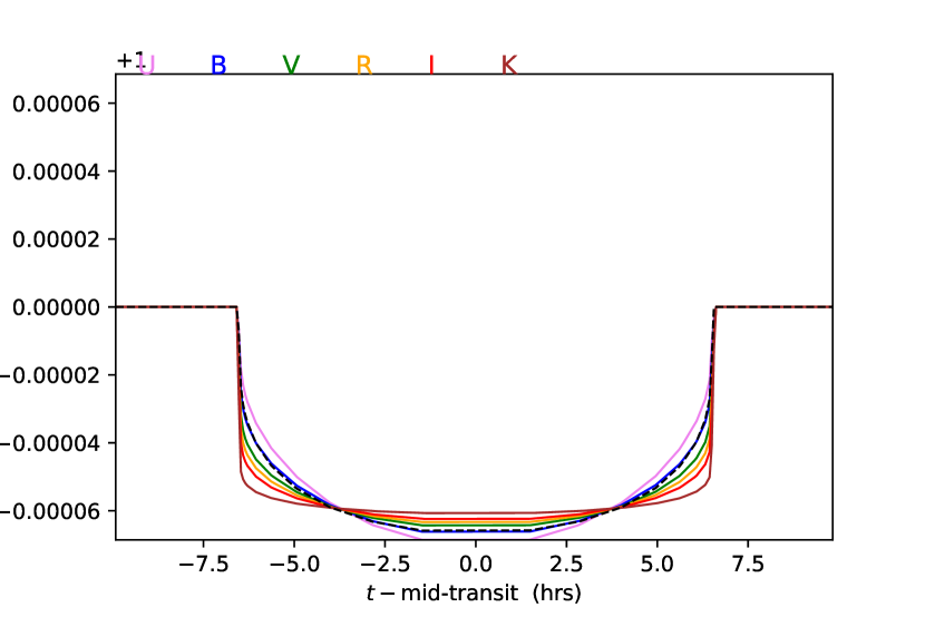
Figure 1: $F^{\rm T}_{{\rm band},i}/F_{\rm band}$ vs. $t$ curves for the Johnson-Bessel $UBVRIK$ bands, calculated at 28 points (solid lines) for the case of a solar host star and a planet of Earth’s radius. A comparable analytic $V$-band interior lightcurve based on the four-parameter limb-darkening law of Claret (2000) is also included for the adjustment parameter $f=2/\pi$ (dashed line, see text).

4 Implementation in CSPy

Transit set-up is controlled with the addition of the ”rOrbit” and ”rPlanet” settings in the Input.py command file to set the values of $R_{\rm orb}$ and $r$, respectively. Additionally, the transit is controlled by a number of previously established settings that have other purposes: the ”logg” and ”massStar” settings are used to compute $R$ and $V_{\rm orb}$, and the ”rotI” setting for rotational broadening is used to compute $b_{\rm min}$.

Currently, CSPy’s radiation field discretization uses the 11 zero-positive abscissae of a 21-point Gauss-Legendre quadrature to sample the $\theta$ polar angle coordinate, and thus the $b$ offset from the substellar point, and that is the maximum number of points sampling a half-transit for the case of $i=\pi/2$ RAD ($b_{\rm min}=0$). The full interior light curve is sampled with twice this number of points (22), and the three-point treatment of ingress and egress bring the total number of points sampling the entire light curve to 28, including the two bracketing un-occulted points. This relatively modest number has been chosen because responsiveness in a Python IDE is a priority that distinguishes CSPy from more realistic FORTRAN atmospheric and spectrum modelling codes. The Thetas.thetas() module in the Chroma+ suite is set up so that it is straightforward to change the order of the Gauss-Legendre quadrature and, thus, the number of points sampling the lightcurve.

References

- Castelli & Kurucz (2006) Castelli & F. Kurucz, R. L., 2006, A&A, 454, 333
- Claret (2000) Claret, A., 2000, A&A, 363, 1081
- Johnson (1965) Johnson, H., L., 1965, ApJ, 141, 923
- Johnson et al. (1966) Johnson, H. L., Mitchell, R. I., Iriarte, B. & Wisniewski, W. Z., 1966, Comm. Lunar Planet. Lab., 4, 99
- Mandel & Agol (2002) Mandel, K. & Agol, E., 2002, ApJ, 580, L171
- Neilson et al. (2017) Neilson, H.R., McNeil, J.T., Ignace, R. & Lester, J.B., 2017, ApJ845, 65
- Short & Bayer (2018) Short, C.I. & Bayer, J.H.T., 2018, arXiv:1805.03674
- Short, Bayer & Burns (2018) Short, C.I., Bayer, J.H.T. & Burns, L.M., 2018, ApJ, 854, 82