An Uncertainty Management Framework for Integrated Gas-Electric Energy Systems

Abstract

In many parts of the world, electric power systems have seen a significant shift towards generation from renewable energy and natural gas. Because of their ability to flexibly adjust power generation in real time, gas-fired power plants are frequently seen as the perfect partner for variable renewable generation. However, this reliance on gas generation increases interdependence and propagates uncertainty between power grids and gas pipelines, and brings coordination and uncertainty management challenges. To address these issues, we propose an uncertainty management framework for uncertain, but bounded gas consumption by gas-fired power plants. The admissible ranges are computed based on a joint optimization problem for the combined gas and electricity networks, which involves chance-constrained scheduling for the electric grid and a novel robust optimization formulation for the natural gas network. This formulation ensures feasibility of the integrated system with a high probability, while providing a tractable numerical formulation. A key advance with respect to existing methods is that our method is based on a physically accurate, validated model for transient gas pipeline flows. Our case study benchmarks our proposed formulation against methods that ignore how reserve activation impacts the fuel use of gas power plants, and only consider predetermined gas consumption. The results demonstrate the importance of considering uncertainty to avoid operating constraint violations and curtailment of gas to the generators.

I Introduction

Throughout the world, the share of electricity generated from renewable energy sources is rapidly increasing, concurrently with a shift towards using natural gas as the predominant fuel for traditional bulk generation [1]. These trends are both driven by near-term goals to decrease carbon emissions [2], as well as long term plans to progress towards fully renewable electric energy systems [3]. In the United States, technological changes that enable the exploitation of previously inaccessible natural gas resources, such as shale formations, have made this fuel abundant and inexpensive [4, 5]. Conveniently, natural gas-fired generators produce significantly lower carbon dioxide and particulate emissions relative to coal power plants, and are much easier to site, permit, and build than nuclear generating stations [6]. This has placed natural gas as the “transition fuel” in the evolving generation mix, which is viewed as a bridge between the traditional centralized grid and a future sustainable energy system [7, 8, 9].

The advantages of gas-fired generators go beyond reduced cost and emissions, and include the ability to flexibly modulate power production in real time. Single cycle plants can quickly go online and have flexible ramping capabilities that allow for fast modulation of their generation output. They are therefore often used as marginal resources that start and shut down multiple times a day. This capability is viewed as filling the near-term need to compensate for rapid changes in uncontrollable renewable generation [10, 11], but also leads to high-volume changes and short-term uncertainty in natural gas consumption [12]. The characteristics of gas-fired power plants are hence very different from traditional loads on natural gas pipelines, such as local gas distribution companies, who hold firm delivery contracts for steady supply of natural gas [13], or industrial customers, who have time-varying, but predictable gas withdrawals[12, 14]. As gas-fired generation expands to account for nearly 50% of installed electric generation capacity in the U.S., such differences become increasingly problematic, and make the power grid vulnerable to interruptions in the natural gas supply chain [15, 16, 17]. These interruptions increasingly challenge the ability of power grid operators to meet generation demand, maintain operating reserves, and ensure power system reliability [18].

Addressing the risk of natural gas shortfall to electric generators is thus essential, and requires the development of more efficient and reliable decision support tools to manage the impact of more variable and uncertain operations in a secure, economical manner. These new tools must address three important challenges:

First, there is a need for increased coordination and information exchange between gas pipelines and the power grid, particularly to improve transparency and jointly manage constraints of the integrated energy delivery network, which we refer to as the gas-electric system.

Second, the tools must include models that reflect the physics of energy flow in electric grids and natural gas pipelines, which each have their distinct challenges. Because electric grids have minimal inherent storage, grid operators must balance generation with load at all times [19], which makes it challenging to secure the system against large outages or fluctuations in renewable energy. The fast system dynamics of electric grids enables power flow in these systems to be accurately represented using steady-state power flow models. Natural gas pipelines, on the other hand, have significant energy stored internally in the form of the transported gas, and can sustain unbalanced operations over hours or days [20]. However, representing this behavior requires modeling of transient gas dynamics, which present modeling and computation challenges.

Third, because gas-fired generators are essential in balancing variations in renewable energy, there is a need for tools that enable uncertainty management across the interface between gas and electricity networks. Specifically, power grid operators must know how they can control gas-fired generators to ensure balance in the electric grid, without adversely impacting the integrity and reliability of natural gas pipelines. Because renewable energy uncertainty occurs at the time-scale of intra-day operation, where natural gas systems are not in steady-state, it is crucial that the model accurately captures the impact of uncertainty on the transient gas dynamics.

Previous studies, which we review extensively in the next section, have considered several of the above aspects. However, to the best of our knowledge, there are no existing methods that constructively address integrated optimization of natural gas and electricity delivery considering transient natural gas dynamics and uncertainty from renewable energy. Combining these three aspects is essential for developing effective decision support tools. Unfortunately, the simultaneous consideration of joint optimization, uncertainty, and transient gas flows creates very challenging non-convex, large-scale problems. In this study, we address this open challenge.

Specifically, the main contribution of our study is to propose the first method for operational scheduling of gas-electric energy systems that jointly considers integrated optimization, coordinated uncertainty management, and gas pipeline transients. The core idea of our framework is simple, but powerful. Our method determines three natural gas consumption profiles corresponding to the scheduled, minimum, and maximum gas withdrawals for each gas-fired generator at each point in time. These three profiles are obtained from the solution of a joint optimization framework for the integrated gas-electric system. In the power system, the gas withdrawal profiles represent the range of available flexibility from the gas-fired generators. By utilizing a chance-constrained optimization formulation for power system operations, we can guarantee (with a high probability) that these withdrawal profiles are consistent with the need for reserve activation in the electric grid. In the natural gas pipelines, the gas withdrawal profiles represent acceptable uncertainty in consumption. Given the maximum and minimum profiles, we apply recent monotonicity results [21, 22, 23] to formulate robust feasibility conditions for the transient natural gas flow dynamics. By including these robust feasibility conditions in the joint optimization, we guarantee that any gas withdrawal profile between the maximum and minimum profiles will not violate the gas system constraints. Thus, by enforcing feasibility for only three gas withdrawal profiles, we are able to guarantee viability of our solutions for a wide range of practical operational scenarios.

We wish to highlight that the formulation of a tractable intra-day optimization problem that simultaneously considers the impact of uncertainty both in the electric grid and gas pipeline transients is nontrivial and novel. Crucially, the formulation leverages recent monotonicity results for transient gas pipeline flows, which enable a new approach to robust gas network optimization and a simple three-scenario interface for information exchange between gas pipeline and power grid operators.

The remainder of the paper is organized as follows. In Section II we provide a detailed review of related work from the quickly evolving literature on gas-electric system coordination, with sections dedicated to each of the three challenges of coordination and integrated optimization, modeling of the transient natural gas dynamics, and uncertainty management. Section III summarizes the conclusions from our literature review and provides an overview of the framework for modeling and coordination of electric grids and natural gas pipelines under uncertainty, based on uncertain, but bounded gas withdrawals. Section IV describes the modeling and optimization framework for multi-period, chance-constrained power system scheduling. In Section V, we provide an overview of the modeling and optimization of large-scale natural gas pipelines, before we describe the extension to robust optimization utilizing monotone systems properties. Based on the formulations provided in the previous sections, Section VI details the coupling between the two systems, determined by the gas-fired generators and the energy and reserves they are scheduled to provide, and presents the mathematical model for joint scheduling and uncertainty management. Section VII outlines the framework we utilize to assess the performance of the method, as well as two benchmark formulations. The numerical results presented in Section VIII demonstrate the performance of the method, and show that accounting for uncertainty of the gas withdrawals is essential for reliable delivery of both gas and electricity. Section IX summarizes and concludes.

II Review of Interactions between Electric Energy Systems and Natural Gas Pipelines

As the bulk electric power system increasingly relies on gas-fired generation, it becomes critical to study the interactions between these complex networked systems, and develop adequate modeling and optimization techniques to coordinate and manage the integrated gas-electric system. In this section we review key issues relating these interacting infrastructure systems, as well as recent academic literature and industry studies. We divide our review into three parts corresponding to the three challenges identified in the introduction, namely A) optimization and coordination of the integrated system, B) modeling of transient gas flow dynamics, and C) uncertainty management.

II-A Integrated Optimization and Coordination of Electric and Natural Gas Transmission Networks

Current interactions between natural gas and electric systems are primarily driven by the electricity demand from natural gas fired power plants. Because gas-fired power plants do not store fuel onsite, gas is a “just-in-time” fuel that must be continuously available in operation. Fuel supply interruptions thus incur a risk of simultaneous outage of multiple gas-fired generators. This has led to growing concerns about inter-sector coordination [18, 24, 25], leading to regulatory action in the U.S. [26]. The situation is particularly challenging because power plants often do not hold firm contracts for pipeline transportation, and are not guaranteed access to sufficient pipeline capacity to transport the gas needed for generation. Instead, gas-fired generators typically rely on shorter-term arrangements in the gas pipeline capacity release market. Thus, in periods when pipeline capacity is subscribed entirely by firm contract holders (e.g., during very cold weather), power plants are the first loads to be curtailed [27].

II-A1 Optimization of Electric Grid Operations

The fuel usage of these gas generators is determined primarily by the production schedules created in day-ahead electricity markets. In the U.S., these markets are cleared by independent (electric) system operators (ISOs) that solve unit commitment, reserve allocation, and economic dispatch problems based on optimal power flow (OPF) formulations [28, 29, 30]. The optimization based markets give rise to electricity prices that are consistent with the physical capacity of the power grid, and have enabled much more efficient utilization of generation and transmission assets [31, 32, 33]. The paradigm in power grid operations is integration of market clearing, scheduling, and operations by standardized optimization-based decision support.

II-A2 Optimization of Natural Gas Pipeline Operations

As the use of natural gas for electricity generation continues to increase, it is important to increase responsiveness and efficiency of natural gas pipeline operations, particularly as the development of new infrastructure slows [34, 35]. Historical load and price analysis in the U.S. natural gas markets indicates that price spikes occur when load levels approach 75% of firm contract capacity [24], which is conventionally taken as the constraint capacity threshold [36]. The prevailing paradigm of pipeline operations is the to conduct marketing, scheduling, and physical gas control operations as separate activities, often using labor intensive experience-based approaches developed by individual companies. One path to more responsive and efficient operation of gas pipelines is the integration of markets and physical control using optimization-based decision support systems analogous to those used in electricity markets. In gas pipeline systems, flow is controlled using compressors and regulators that directly change pressures and flow rates, or by scheduling injection and consumption of gas. Optimization-based scheduling of pipeline system operations can provide location- and time-dependent prices for natural gas that account for pipeline flow physics, engineering limitations, and operational constraints [37, 38, 39]. This would allow gas-fired generation asset managers to provide bids and offers that reflect their price-sensitive demand [40]. Advancing pipeline operations methods will also increase reliability in supplying fuel to the electric power sector during highly loaded conditions [41]. This may become increasingly important in the future, when power-to-gas technology, which converts excess renewable energy into gas, may further strengthen interactions between the two systems and aggravate associated reliability issues [42, 43, 44, 45].

II-A3 Integrated Optimization of Electric and Natural Gas Networks

To ensure a power system dispatch that respects gas pipeline feasibility constraints, several studies have considered the inclusion of gas pipeline models in power grid design and operation analysis, forming methods for integrated optimization and operational planning [46, 47, 48]. Multiple subsequent studies on joint optimization have considered electric grid scheduling subject to security constraints that arise from the dependence on gas pipelines [49, 50, 51, 52, 53, 54, 55, 56, 41, 57, 58, 59, 60], aiming for improved power grid resilience [61, 62], better robustness against $N-1$ failures [63, 64, 65], or consideration of joint expansion planning [66, 67, 68, 69, 70, 71, 72]. These studies have indicated that there would be substantial economic and reliability advantages to improving coordination between the sectors [73, 74, 75].

II-A4 Information Exchange as a Barrier to Coordination

Better coordination between natural gas and electric energy system managers can improve the reliability of both sectors. However, institutional and regulatory barriers typically prevent sharing of the necessary operational data, which is considered proprietary or competitive information. It is therefore unlikely that a single entity will be able to collect the network models and operational information required for joint optimization of both systems. This has led to the study of coordinated operations that rely only on the limited exchange of financial and operational information [37, 76, 40, 77], including constraints on the gas stored in pipelines [78, 79]. Other studies have examined various coordination market mechanisms and bidding strategies [80, 81, 82, 83], including models that account for future energy system functions [84, 85]. However, methods for coordination with limited information exchange subject to uncertainty remain limited.

II-B Transient Natural Gas Pipeline Dynamics

An important difference between the power grid and natural gas pipelines involves the time-scales of system dynamics. While power flow in transmission lines reaches steady-state within seconds, natural gas pipelines typically never reach steady-state in intra-day operations [86]. The inertia and slow dynamics of gas flow are advantageous for several reasons. Flows are constant on the second time scale of electro-mechanical transients in the power grid, leaving operators time to react to contingencies before their effects propagate through the system [87, 63]. Because of their slow dynamics and ability to store a substantial mass of gas internally, pipelines are in many ways similar in function to grid-scale batteries [88]. The energy stored is reflected in a higher-than-minimum pressure, and is typically referred to as “linepack”. This storage capability enables gas-fired generators to withdraw gas in excess of the scheduled rate for a limited duration without violating pipeline operating limits. This ability to “pack and draft” gas in a pipeline is captured only by dynamic models.

While the linepack provides short-term flexibility, the slow evolution of the gas pipeline state also implies that gas controllers must take a proactive role in predicting future system states and take action to prevent negative impacts of potential future disturbances, utilizing metrics such as pressure cover [89]. Predicting the evolution of pipeline system pressures can be done using dynamic gas pipeline optimization or simulations, where partial differential equations (PDEs) describe how pressures, densities and mass flows evolve over time as a function of natural gas withdrawals and operation of compressor stations. This dynamic behavior is critical to understand the impact of both generation and compressor schedules [41, 90], renewable fluctuations [12, 14], and contingencies [63] on gas pipeline operations. However, because of the theoretical and computational challenges associated with PDE constrained optimization, a majority of the research on the interactions between natural gas and electric systems have utilized steady-state equations and approximations thereof, particularly when considering renewable energy uncertainty [91, 92, 93, 94].

In the following, we review the steady-state and transient dynamic models of the natural gas system in more detail.

II-B1 Steady-State Optimization

Although the steady-state is typically never reached in intra-day operations, steady-state approximations, such as the Weymouth equations [95], are frequently utilized in the academic literature as a basis for gas pipeline modeling and optimization (including many of the above and subsequent references). Steady-state optimization of gas pipelines, utilizing the steady-state equations, has been formalized in optimal gas flow (OGF) problems [96, 97, 98, 95, 99]. The constraints are non-linear algebraic equations, which are easier to solve than the time-dependent PDEs that describe transient pipeline behavior. However, the steady-state models, or sequences of such models, are insufficient to capture the effect of linepack [20, 55]. Furthermore, the steady-state equations (or relaxed version thereof) do not capture the phenomena needed to guarantee feasibility under dynamic conditions [41], and may not utilize the pipeline capacity to the greatest possible extent.

II-B2 Transient Optimization

To address the shortcomings of the steady-state natural gas models, it is important to develop optimization methods that are able to account for the transient dynamic system behavior. Transient optimization, frequently also referred to as dynamic optimization, includes the PDE representation of the gas pipeline dynamics. These models have been expressed as model predictive optimal control problems [100, 101, 102, 103, 90, 104, 105, 106, 107, 108], or solved using adjoint optimization [109].

The PDE constraints that represent the transient gas flows complicate the transient optimization problems [110], and make them notoriously difficult to simulate and optimize in a tractable way [111, 100, 112]. Extension to general network structures, scalability of the computational methods, and accuracy of models and solutions continue to present challenges. However, recent work has made advancements towards tractable, rapid pipeline transient optimization [111, 100, 113, 90, 104, 114, 115, 116, 117]. In particular, these recent studies have resulted in modeling concepts and dynamic system representations for general large-scale pipeline systems [113, 118], optimal control formulations [90], algorithms based on adjoint optimization [109], comparisons of various discretization schemes [116, 117], extension to non-ideal gas modeling [119], as well as validation of simulation and optimization approaches with respect to industrial data and commercial solvers [37]. Collectively, these developments can enable widespread adoption of transient gas pipeline models.

II-C Uncertainty Management in Gas-Electric Energy Systems

Both electric grids and natural gas pipeline systems experience uncertainty in the demand and supply of energy. Flexible gas-fired generators are frequently used to balance real-time fluctuations in the electric grid. Uncertainty and variability in power systems thus propagates into the natural gas pipelines. We review methods for managing this uncertainty in power grids, gas pipeline systems, and the integrated energy system.

II-C1 Uncertainty in Electric Power Systems

With increasing levels of renewable energy generation, the grid is experiencing both increased short-term variability and uncertainty. This has led to the development of uncertainty-aware optimization methods for power systems operation, in particular stochastic and robust approaches for unit commitment and optimal power flow problems. These methods include, among many others, robust and worst-case methods [120, 121, 122, 123], two- and multi-stage stochastic programming based on samples [124, 125, 126, 127], stochastic approximation techniques [128], and chance-constrained formulations [129, 130, 131, 132, 133, 134, 135, 136, 137, 138, 139, 140]. Many of these methods consider the co-optimization of energy and reserve capacity.

II-C2 Uncertainty in Natural Gas Networks

Increased integration of uncontrolled and variable wind generation into a power system translates into more uncertainty and variability in natural gas demand from gas-fired generating units [11, 14, 12]. Variable generation schedules and reserve activation from gas-fired generators lead to a propagation of uncertainty from the power grid to gas pipelines [141, 142]. Several studies have investigated how this uncertainty and variability impacts gas pipelines [143, 12, 14, 144, 145, 91]. In addition to the impact of renewable energy variability [79, 146], natural gas pipelines are also influenced by uncertainty in the consumption of traditional pipeline customers [147], failures of components such as compressors or pipelines [63, 64, 65], and uncertainty regarding available pipeline capacity [148].

II-C3 Integrated Uncertainty Management

The advantages of coordinated scheduling have inspired methods for joint management to mitigate the propagation of uncertainty from the electric grid to natural gas pipelines. Several studies have formulated power system scheduling problems that account for these factors. Some of these methods consider sequential optimization, where additional constraints are added to the electric scheduling problem when gas pipelines experience constraint violations [149, 79], while others consider joint optimization problems. A common approach to joint optimization is to model wind generation as stochastic and uncertain, and develop two-stage stochastic formulations for joint gas and electricity system operations [150, 151, 92, 93, 94]. Other approaches use interval optimization [152] or draw on robust optimization techniques [153, 154, 155, 156, 64, 157, 158]. Most of these studies consider operational scheduling, and some include emerging power-to-gas technologies [154, 159, 160, 161] or expansion planning [162, 156, 64].

Solving the resulting problems can be challenging, particularly if the number of considered scenarios is large. This can be the case in scenario-based stochastic formulations, which may require a large number of scenarios to obtain accurate solutions, as well as in robust formulations that generate constraints based on, e.g., identification of worst-case scenarios [157], Benders cuts [151], or using column-and-constraint generation [153, 156]. We also note that the method for robust co-optimization proposed in [154] uses ADMM to facilitate optimization with limited information exchange. While the above literature provides a valuable set of methods for joint uncertainty management, and some also addresses questions related to limited information exchange, none of these methods include a transient dynamic PDE model of the natural gas flows. This is problematic because renewable energy uncertainty occurs at the time-scale of intra-day operation, where natural gas systems are not in steady-state. It is therefore important that the model accurately captures the impact of uncertainty on the transient gas dynamics.

In the next section, we discuss the gap identified in our review, and propose a framework to address this shortcoming.

III Framework for Coordinated Scheduling Under Uncertainty

Our review highlights the benefits and challenges of coordination between natural gas and electric systems. Successful coordination schemes require tractable joint optimization models that also account for practical constraints such as clearly defined interfaces, as well as important physical characteristics such as time-evolution and linepack that are only captured in a transient model. Furthermore, to ensure that gas-fired generators can reliably provide balancing for intermittent renewables, it is necessary to develop a framework for coordinated scheduling under uncertainty. In our review, we note a lack of methods for integrated optimization and uncertainty management that also considers transient gas dynamics.

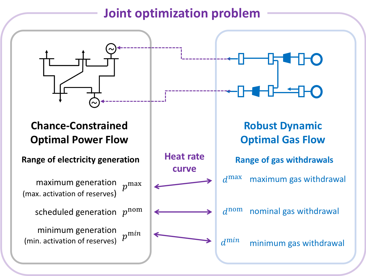
Figure 1: Schematic overview of the joint optimization framework. The framework combines chance-constrained optimal power flow with robust dynamic optimal gas flow, and determines feasible ranges of gas withdrawals from gas-fired power plants.

To address this knowledge gap, we propose a practical framework for coordinated gas-electric scheduling which incorporates rigorous safety guarantees for a range of uncertain operating conditions, a transient model of the gas pipeline, and clearly defined interfaces between the two systems.

The proposed framework is based on the simple principle that the electric and natural gas systems agree on a range of admissible gas withdrawals for each gas generator. These ranges are formulated as maximum and minimum gas consumption profiles for each gas-fired power plant, at each point in time. For the electric grid the maximum and minimum gas withdrawals corresponds to maximum and minimum limits on electricity generation. The conversion from admissible gas withdrawals to admissible electricity generation range is done using the generator heat rate curve. Our proposed method is able to determine maximum and minimum gas withdrawals that (i) are consistent with the needs for generation and reserve activation in the electric power grid, and (ii) guarantee robust feasibility of the gas system for any intermediate withdrawal. The three parts of the method, which are all combined in one joint optimization problem, are illustrated in Fig. 1, and summarized below.

To identify an optimal generation dispatch and reserve allocation for the electric grid, we utilize a probabilistic power system optimization method that ensures balanced power system operation and manages transmission line congestion under uncertainty. In our framework, any multi-period stochastic or robust methods for electric grid scheduling can be utilized, as long as the scheduling algorithm provides an upper and lower bound on the gas-fired generation at each point in time. For our implementation in this paper, we propose to use a chance-constrained optimal power flow formulation that co-optimizes generation dispatch and reserve allocation for each generator. The chance constraints are reformulated using an analytical approach [131, 134]. This method has been shown to be effective and scalable [138, 163], and relates well to existing industry practice [164]. The details of this method are described in Section IV.

The power system optimization problem is coupled with the gas system optimization problem through the heat rate curve, which transforms the nominal, maximum and minimum generation outputs (corresponding to scheduled generation and full activation of upwards or downwards reserves, respectively) into nominal, maximum and minimum gas withdrawals for each generator. These uncertain, but bounded gas withdrawals are combined into three scenarios for gas pipeline operation corresponding to 1) all generators operating at nominal generation, 2) all generators consuming the maximum amount of gas, and 3) all generators consuming the minimum amount of gas. Together, these three scenarios describe the interface between the two systems. Details of how the integration of the natural gas and electric models are given in Section VI.

To guarantee robust feasibility for the gas system, we utilize recent results for gas flow monotonicity [21, 22, 23] to formulate a robust transient gas flow optimization. This step is an important novelty of our proposed method, as we are able to guarantee feasibility for a wide range of practical operating scenarios, while considering no more than three scenarios within the optimization problem. The formulation of the transient dynamic gas optimization and the extension to a robust formulation are described in Section V.

The main advantages of the proposed method are:

• By guaranteeing that any gas withdrawal within the determined maximum and minimum bounds is feasible, we allow gas-fired generators to vary their electricity production to balance loads in the power system, without risking curtailments in the gas supply or cause constraint violations in the gas pipeline system.

• Feasibility is guaranteed for a wide range of operating scenarios in the coupled gas-electric system, while only considering three scenarios for the natural gas withdrawals.

• The a small number of required scenarios enables tractable optimization problems, even when considering the transient dynamic gas flows.

Our method expands upon existing literature by considering both transient dynamics and uncertainty in an integrated optimization problem. Based on our review, addressing these aspects together is nontrivial and novel. To our knowledge, previous studies on joint optimization under uncertainty [150, 151, 152, 155, 162, 64, 157, 154, 159, 92, 153, 158, 94, 93, 156, 160, 161] consider only steady-state gas models.

The details of the mathematical model, which considers the chance-constrained optimal power flow and robust dynamic gas flow problem as one integrated optimization problem, are given in the following sections. In the interest of clarity, we first separately introduce the models for the electric power system and the natural gas network, before combining them into an integrated model. We first start with the chance-constrained power system model, where we discuss reserve scheduling in detail. We then move on to gas pipeline analysis, where we first describe the deterministic transient optimization model, and then discuss our extensions to a robust optimization formulation. Finally, we discuss how we model the interactions between the systems using the heat rate curve, and formulate the proposed integrated optimization for gas-electric systems.

IV Chance-Constrained Optimal Power Flow for Generation and Reserve Scheduling

In this section we describe a method for probabilistic optimization of electric transmission systems with high penetrations of renewable energy, which guarantees constraint satisfaction with a high probability. This guarantee is naturally enforced using chance constraints, giving rise to a multi-period, chance-constrained optimal power flow problem. While the formulation is mostly a review of pre-existing work [131, 134, 138, 163], we include a more in-depth discussion of reserve scheduling. Using chance constraints for reserve scheduling aligns well with probabilistic criteria for reserve dimensioning used within ENTSO-E [165, 164], which requires the reserve capacities to be sufficiently large to cover imbalances with a high probability. For example, the Swiss market for ancillary services [164] constructs an empirical probability distribution based on historical power imbalances and enforces a chance constraint in the market clearing to ensure that the procured reserve capacities will exceed the required reserve activation with a predetermined probability. Our approach formalizes this method for reserve scheduling, and includes probabilistic feasibility guarantees for line flows as well.

IV-A Power System Network Modeling

Let $G_{P}=(\mathcal{V}_{P},\mathcal{E}_{P})$ denote the graph of the power transmission network, where $\mathcal{V}_{P}$ is the set of nodes (i.e., buses) with $|\mathcal{V}_{P}|=m$ and $\mathcal{E}_{P}$ is the set of edges (i.e., transmission lines) of the system with $|\mathcal{E}_{P}|=n$. All quantities associated with a line from bus $i$ to bus $j$ are identified by subscript $ij$. Let $\mathcal{G}$ denote the set of generators in the network. For simplicity of notation, we assume that there is exactly one generator with production $p_{i}(t)$ and one load with consumption $h_{i}(t)$ per node, such that $|\mathcal{G}|=|\mathcal{V}_{P}|=m$.

IV-A1 Modeling Uncertain Demand

The source of uncertainty in our model is power injection uncertainty, i.e., how much power will be injected into or withdrawn from the system by uncontrollable sources such as renewable energy generators or loads.

We denote the forecasted demand for power at each node $h_{i}(t)$ as continuous demand functions defined for $0\leq t\leq T$ where $T=24$ hours. To model uncertainty regarding the actual demand, we express each power injection in the system as

$$\tilde{h}(t)=h(t)-\omega(t).$$ (1)

Here, $\tilde{h}(t)$ denotes the vector of all real-time loads in the system at time $t$. The vector $h(t)$ is the forecasted system load, and $\omega(t)$ correspond to the difference between the forecasted and actual load. Since the actual load is not known until real-time operations, the exact value of $\omega(t)$ is unknown and we will refer to $\omega(t)$ as the uncertain part nodal demand. Note that $\omega(t)$ can represent uncertainty arising from either load or renewable energy fluctuations, or a combination of both. We also assume that the covariance matrix $\Sigma(t)$ of $\omega(t)$ is known and finite. The total difference between forecasted and actual load is referred to as the total real-time power imbalance, which we denote by $\Omega(t)$ and define as

$$\Omega(t)=\sum_{i\in\mathcal{V}_{P}}\omega_{i}(t).$$

IV-A2 Power Balancing in Real-Time Operations

An important aspect of power system operations is to maintain balance between the power produced by the generators and the power consumed by the loads at all times. To ensure that power balance is maintained in real-time operation, the changes in the total load, represented by the imbalance $\Omega(t)$, are compensated through the activation of reserves. In this process, conventional generators are asked to either increase or decrease their power generation to match the power consumption of loads in real time. Following standard conventions for power system balancing implemented in, e.g., the automatic generation control (AGC), we assume that activation of reserves by individual generators is given by a vector of participation factors $\beta$ that describe how much each generator contributes to compensate for the imbalance $\Omega(t)$. The participation factors give rise to a policy for generation control of the form

$$\tilde{p}(t)=\bar{p}(t)-\beta(t)\Omega(t).$$ (2)

In this policy, $\bar{p}(t)$ represents the vector of scheduled power generation, while the term $-\beta(t)\Omega(t)$ represents real-time adjustments in the output, referred to as activation of reserves.

Assuming a lossless DC power flow approximation of the system, total power balance requires that the total generation equals total demand for any realization $\omega(t)$, i.e.,

$$\textstyle\sum_{i\in\mathcal{G}}\left(p_{i}(t)-\beta_{i}\Omega(t)\right)-\sum_{j\in\mathcal{V}_{P}}\big{(}h_{j}(t)-\omega_{j}(t)\big{)}=0.$$ (3)

This constraint can be rearranged into the expression

$${\textstyle\sum_{i\in\mathcal{G}}p_{i}(t)-\sum_{j\in\mathcal{V}_{P}}h_{j}(t)+\left(1-\sum_{i\in\mathcal{G}}\beta_{i}\right)\Omega(t)=0.}$$

Here, the first two terms enforce power balance for the forecasted operating point, while the last term ensures power balance during fluctuations. To guarantee power balance for any realization of $\Omega(t)$, we enforce the conditions

$$\sum_{i\in\mathcal{G}}p_{i}(t)-\sum_{j\in\mathcal{V}_{P}}h_{j}(t)=0,\quad \forall~{}t\in T,$$ (4a)

$$\sum_{i\in\mathcal{G}}\beta_{i}(t)=1,\quad\beta_{i}(t)\geq 0\quad \forall~{}i\in\mathcal{G},~{}t\in T.$$ (4b)

In some power systems, the participation factors $\beta$ remain fixed for prolonged periods of time. We will assume that they can be updated at every scheduling interval (e.g., for every hour in the day-ahead market clearing), and that they are co-optimized along with the procurement of reserves.

IV-B Reserve Scheduling as a Chance Constraint

Reserve scheduling determines the reserve capacities $r^{+}_{i}$ and $r^{-}_{i}$ for each generator $i$. Probabilistic reserve scheduling ensures that (i) the generators have the physical capacity required to provide reserve activation, and (ii) the total up-reserve and down-reserve capacities $r^{+}$ and $r^{-}$ are sufficiently large to make up for the power imbalances. Since the real-time power unbalance $\Omega(t)$ is a random variable, these requirements cannot be enforced as deterministic constraints. Instead, we follow industry practice [164] and previous results [138] to ensure that the reserve capacity is sufficient with a high probability.

IV-B1 Reserve Sufficiency for Individual Generators

To ensure that each individual generator $i\in\mathcal{G}$ has sufficient capacity available to provide reserve activation, we formulate the generator constraints as

$$\begin{matrix}\bar{p}_{i}(t)+r_{i}^{+}(t)\leq p_{i}^{\max},~{}~{}\forall~{}i\in\mathcal{G},~{}t\in\mathcal{T}\\ \bar{p}_{i}(t)-r_{i}^{-}(t)\geq p_{i}^{\min},~{}~{}\forall~{}i\in\mathcal{G},~{}t\in\mathcal{T}\end{matrix}\,\,$$ (5)

$$\begin{matrix}\mathbb{P}_{\Omega}(-\beta_{i}(t)\Omega(t)\leq~{}~{}r_{i}^{+}(t))\geq 1-\varepsilon,~{}~{}\forall~{}i\in\mathcal{G},~{}t\in\mathcal{T}\\ \mathbb{P}_{\Omega}(-\beta_{i}(t)\Omega(t)\geq-r_{i}^{-}(t))\geq 1-\varepsilon,~{}~{}\forall~{}i\in\mathcal{G},~{}t\in\mathcal{T}\end{matrix}\,\,$$ (6)

$$r_{i}(t)^{+}\geq 0,~{}~{}r_{i}(t)^{-}\geq 0,~{}~{}\forall~{}i\in\mathcal{G},~{}t\in\mathcal{T}$$ (7)

The first two constraints (5) ensure that the combination of the scheduled generation $p_{i}(t)$ and reserve capacities $r_{i}^{+},r_{i}^{-}$ remain within the upper and lower generation limits $p_{i}^{\max},p_{i}^{\min}$. The latter two constraints (6) enforce that the activated reserves do not exceed the scheduled reserve capacities $r_{i}^{+},r_{i}^{-}$ with probability $1-\varepsilon$, for each generator $i$. These type of constraints are referred to as individual chance constraints, as they consider each generator individually. Eq. (7) ensures that the reserve capacities are positive.

Note that the reserve constraints in (6) are a chance constrained version of hard constraints on generation output, which is directly controllable. In reality, a generator may not alter its generation by more than the procured reserve capacity (and certainly never produce beyond the maximum generation capacity $p^{\max}$, which is physically impossible). A chance-constraint violation therefore does not imply a generator overload, but rather describes the probability that the simple affine policy for reserve activation described in 2 is no longer working. Instead, the system operator must resort to alternative controls to maintain power balance. This setting has been studied in detail [166].

In addition to the above constraints, the problem must take into account of fast the generators are able to modulate their output. To ensure that the generators scheduled for reserves are physically capable of delivering them, system operators typically test generators to ensure that they are able to follow reserve activation signals. The reserves procured from each generator must lie within the maximum capacity that the generator has been certified for:

$$0\leq r^{+}_{i}(t)\leq r^{+}_{i,\max},$$ (8a)

$$0\leq r^{-}_{i}(t)\leq r^{-}_{i,\max},\quad\forall i\in\mathcal{G},t\in\mathcal{T},$$ (8b)

Here, $r^{+}_{i,\max},r^{-}_{i,\max}$ denote the maximum up and down reserve capacity of generator $i$. Finally, the change in generation set points between two consecutive time periods must lie within the ramping limits of the generator,

$$\bar{p}_{i}(t)-\bar{p}_{i}(t+1)\leq R^{\max}_{i},$$ (9a)

$$\bar{p}_{i}(t+1)-\bar{p}_{i}(t)\leq R^{\max}_{i},\ \forall i\in\mathcal{G},t\in\mathcal{T}.$$ (9b)

IV-B2 Reserve Sufficiency for the Overall System

While each generator needs sufficient capacity to provide the requested reserves, it is also more important to ensure that the total amount of scheduled reserve capacity from all generators is sufficient for balancing. This can be expressed as the following joint chance constraint,

$$\mathbb{P}_{\Omega}\begin{pmatrix}-\beta_{i}(t)\Omega(t)\leq~{}r_{i}^{+}(t),\,\forall~{}i\in\mathcal{G}\\ -\beta_{i}(t)\Omega(t)\geq-r_{i}^{-}(t),\,\forall~{}i\in\mathcal{G}\end{pmatrix}\geq 1-\varepsilon_{joint},\,\forall\,t\in\mathcal{T}$$ (10)

This constraint guarantees that the reserve activation is within the scheduled reserve capacities for all generators, with probability $1-\varepsilon_{joint}$. This is similar to requirements imposed by system operators, such as Swissgrid [164].

In general, solving problems with joint chance-constraints like (10) is more challenging than solving problems with individual chance constraints like (6). However, using the particular structure of (10), it has been shown [138] that enforcing the single chance constraints (6) gives strong guarantees on the satisfaction of the joint reserve requirement (10). We derive these results here in more detail.

Because the total power imbalance $\Omega$ is a scalar random variable, the individual chance constraints (6) impose a quantile constraint for each generator $i\in\mathcal{{G}}$:

$$\mathbb{P}_{\Omega}\Big{(}\!-\!\beta_{i}(t)\Omega(t)\leq r_{i}^{+}(t)\Big{)}\!\geq\!1-\varepsilon\ \equiv\ -\beta_{i}(t)Q_{\Omega}(\varepsilon)\leq r_{i}^{+}(t),$$

$$\mathbb{P}_{\Omega}\Big{(}\beta_{i}(t)\Omega(t)\leq r_{i}^{-}(t)\Big{)}\!\geq\!1-\varepsilon\ \equiv\ \beta_{i}(t)Q_{\Omega}(1-\varepsilon)\leq r_{i}^{-}(t)$$

where $Q_{\Omega}(\varepsilon)$ denotes the $\varepsilon$-quantile of the random variable $\Omega$. Note that while we have two constraints for each generator, the values of $Q_{\Omega}(\varepsilon)$ and $Q_{\Omega}(1-\varepsilon)$ are shared among all the constraints. Therefore, the above constraints are equivalent to requiring that the ratio between the reserve capacities $r^{+}_{i},r^{-}_{i}$ and the participation factors $\beta_{i}$ for all generators satisfy

$$\max_{i\in\mathcal{G}}-\frac{r_{i}^{+}(t)}{\beta_{i}(t)}\leq Q_{\Omega}(\varepsilon)\leq Q_{\Omega}(1-\varepsilon)\leq\min_{i\in\mathcal{G}}\frac{r_{i}^{-}(t)}{\beta_{i}(t)}.$$ (11)

As a result, (6) are satisfied for all $i\in\mathcal{G}$ if and only if (11) is satisfied. Further, by definition of the quantile, (11) is satisfied if and only if

$$\mathbb{P}_{\Omega}\Big{(}\!-\!r_{i}^{+}(t)\leq\beta_{i}(t)\Omega(t)\leq r_{i}^{-}(t),~{}\forall i\!\in\mathcal{G},t\in\mathcal{\!}T\Big{)}\!\geq\!1\!-\!2\varepsilon.$$

which is equivalent to the joint chance constraint (10) with $\varepsilon_{joint}=2\varepsilon$. Therefore, the individual local chance constraints we impose in (6) automatically enforce the global joint chance constraint in (10).

IV-C Transmission Line Constraints

With the DC power flow model, the power flows can be expressed as a linear function of the nodal power injections using the power transfer distribution factors (PTDF) [167],

$$p^{line}_{{\color[rgb]{0,0,0}{mn}}}(t)=M_{({\color[rgb]{0,0,0}{mn}},\cdot)}\left(\bar{p}(t)-\beta(t)\Omega(t)-h(t)+{\omega}(t)\right),$$ (12)

where $p^{line}_{mn}$ denotes the line flow on the transmission line between nodes $m$ and $n$, $M$ is the PTDF matrix as defined in [130] and $M_{(mn,\cdot)}$ denotes the row of $M$ corresponding to line $mn$. This model captures the impact of the uncertain fluctuations and reserve activation on the power flows $p^{line}_{mn}(t),~{}\forall{mn}\in\mathcal{E}_{P}$, which themselves become random variables. Similar to the generation constraints, we take a probabilistic approach and enforce the power flow limits using chance constraints,

$$\mathbb{P}_{\omega}\left(p^{line}_{mn}(t)\leq~{}~{}p_{mn}^{\max}\right)\geq 1-\epsilon_{mn},\quad\forall~{}mn\in\mathcal{L}$$ (13a)

$$\mathbb{P}_{\omega}\left(p^{line}_{mn}(t)\geq-p_{mn}^{\max}\right)\geq 1-\epsilon_{mn},\quad\forall~{}mn\in\mathcal{L}$$ (13b)

with $p^{line}_{{\color[rgb]{0,0,0}{mn}}}$ defined as in (12). Here, (13a) and (13b) enforce the upper and lower bounds on the line flow (corresponding to the maximum line flow in both directions).

The probability of violation in (13) has a different meaning than for the generator constraints in (6). Whereas the generator constraints (6) are hard constraints on variables that are directly controllable, the chance constraints on the power flow (13) correspond to soft constraints on the flow on each transmission line, which is only indirectly controllable. For these chance constraints, a constraint violation implies that a line might experience an actual, physical overload with probability $1-\varepsilon$. Depending on the size and duration of the overload, the operator can either wait for the overload to resolve itself (if it is small and short-lived) or implement alternative control actions, such as manual redispatch, to relieve line congestion.

For the generators, the individual chance constraints (imposed separately on each generator) imply joint satisfaction of the chance constraint. For the line flow constraints (13), this result does not hold, as the constraints depend not only on the total power imbalance $\Omega(t)$, but on the full random vector $\omega(t)$. Therefore, the probability that any line is overloaded is, in the worst case, equal to the number of lines times their individual violation probability, i.e. $\varepsilon_{max}=\max\{n\cdot\epsilon,1\}$. However, given the structure of power grids, the number of line constraints that experiences violations is typically very low [134, 138]. It is therefore possible to very effectively control the joint violation probability using individual chance constraints on the lines.

IV-D Reformulation of the Chance Constraints

The chance-constrained optimization problem (19) can only be solved after reformulation as a deterministic optimization problem. While there are multiple approaches for the chance constraint reformulation, we utilize the analytical reformulation from [131, 134] which is highly scalable [134, 138]. For simplicity, we assume that the forecast errors follows a multivariate Gaussian distribution. However, the same formulation can be extended to account for more general or partially unknown distribution [168] as well as general elliptical uncertainty sets [169].

Specifically, we assume that the uncertainty $\omega(t)$ follow a multivariate Gaussian distribution with a known covariance matrix $\Sigma$ for each time step. For simplicity of notation, we ignore the time-dependency of $\Sigma$ and assume that $\Sigma$ is constant throughout the time horizon. However, in reality the constraints could easily be changed to account for a separate $\Sigma$ at each time step. We assume that we have unbiased forecasts of the load, such that the expected value of $\omega(t)$ is $0$. With the analytical reformulation, the chance constraints (6) for each generator $i$ can be reformulated as linear constraints [170],

$$r_{{\color[rgb]{0,0,0}{i}}}^{+}+\beta_{{\color[rgb]{0,0,0}{i}}}Q_{\Omega}(1-\epsilon)\geq 0,\quad{\color[rgb]{0,0,0}{\forall i\in\mathcal{G}}}$$ (14a)

$$r_{{\color[rgb]{0,0,0}{i}}}^{-}-\beta_{{\color[rgb]{0,0,0}{i}}}Q_{\Omega}(1-\epsilon)\geq 0,\quad{\color[rgb]{0,0,0}{\forall i\in\mathcal{G}}}$$ (14b)

where the quantile $Q_{\Omega}(1-\epsilon)=\Phi^{-1}(1-\epsilon)\sqrt{\bm{1}^{T}\Sigma\bm{1}}$ is a constant. Here, $\Phi^{-1}(1-\epsilon)$ represents the inverse cumulative distribution function of the standard normal distribution evaluated at $1-\varepsilon$ (i.e., the $1-\epsilon$ quantile) and $\bm{1}$ is a vector with entries of one. The transmission line constraints (13) for each line $mn$ are reformulated as second-order cone constraints [134],

$$M_{({\color[rgb]{0,0,0}{mn}},\cdot)}\left(\bar{p}(t)-h(t)\right)+\Phi^{-1}(1-\epsilon)~{}\!s_{{\color[rgb]{0,0,0}{mn}}}\leq p_{{\color[rgb]{0,0,0}{mn}}}^{\max},$$ (15a)

$$M_{({\color[rgb]{0,0,0}{mn}},\cdot)}\left(\bar{p}(t)-h(t)\right)-\Phi^{-1}(1-\epsilon)~{}\!s_{{\color[rgb]{0,0,0}{mn}}}\geq-p_{{\color[rgb]{0,0,0}{mn}}}^{\max},$$ (15b)

$$\text{with }{\textstyle s_{{\color[rgb]{0,0,0}{mn}}}=\sqrt{(M_{({\color[rgb]{0,0,0}{mn}},\cdot)}(I-\beta\mathbf{1}))\Sigma(M_{({\color[rgb]{0,0,0}{mn}},\cdot)}(I-\beta\mathbf{1}))^{T}}}.$$

Here, $s_{{\color[rgb]{0,0,0}{mn}}}$ is a variable representing the standard deviation of the line flows, $I$ is the identity matrix and $\bm{1}$ is the vector with entries of one. For more details on the derivation of these equations, we refer the reader to [138].

IV-E Multi-Period Chance-Constrained Optimal Power Flow

Based on the modeling considerations presented in the previous section, we formalize the generation and reserve scheduling problem as a multi-period, chance-constrained optimal power flow (OPF) problem.

IV-E1 Decision variables

Our chance-constrained OPF model includes the following decision variables,

Generation set points: $$\mathbf{\bar{p}}\equiv\big{(}\bar{p}(t),\ t\in\mathcal{T}\big{)},$$

Up and down reserves: $$\mathbf{r}\equiv\big{(}r^{+}(t),r^{-}(t)\ t\in\mathcal{T}\big{)},$$

Participation factors: $${\bm{\beta}}\equiv\big{(}\beta(t)\ t\in\mathcal{T}\big{)}.$$

IV-E2 Probabilistic Power Flow Constraints

For ease of exposition, we define the constraint set $\Pi$ that a given choice of decision variables $\mathbf{\bar{p}(t),r,\beta(t)}$ must satisfy:

$$\Pi(\mathbf{\bar{p}},\mathbf{r},\bm{\beta})=$$

$$\quad\begin{cases}&\mbox{Total power balance}~{}\eqref{eq:balancing},\\ &\mbox{Generator limits}~{}\eqref{eq:gen_cap},\\ &\mbox{Probabilistic reserve requirement}~{}\eqref{eq:gen_res_ref},\\ &\mbox{Limits on reserve procurement}~{}\eqref{eq:reserve_bid_bounds},\\ &\mbox{Generator ramping limits}~{}\eqref{eq:ramping_limits},\\ &\mbox{Line flow constraints}~{}\eqref{eq:ptdf},\eqref{eq:line_ref}\end{cases}$$

IV-E3 Objective function

The objective function for the power system evaluates the cost of generation and reserves:

$$J_{P}(\mathbf{\bar{p}},\mathbf{r}) =\sum_{i\in\mathcal{G}}\sum_{i\in\mathcal{T}}\bigl{\{}K_{i}p_{i}(t)\bigr{\}}$$

$$\,\,+\sum_{i\in\mathcal{G}}\sum_{i\in\mathcal{T}}\bigl{\{}a_{i}(r_{i}^{+}(t)+r_{i}^{-}(t))\bigr{\}}$$ (18)

Here, $K_{i}$ and $a_{i}$ represent the cost of generation and reserve capacity, respectively.

IV-E4 Multi-period chance-constrained DC OPF

The MP-CCOPF can be compactly formulated as follows:

$$\!\!\min\limits_{\mathbf{\bar{p}},\mathbf{r},\bm{\beta}} J_{P}(\mathbf{\bar{p}},\mathbf{r})$$ Generation and Reserve Cost: (19a)

s.t.: $$\mbox{Power flow constraints:}~{}\Pi(\mathbf{\bar{p}},\mathbf{r},\bm{\beta}).$$ (19b)

V Robust Optimization for
Transient Gas Pipeline Scheduling

In this section we provide an overview of a standardized approach for modeling large-scale gas transmission pipelines for optimal control, which has been applied in several studies [90, 41, 163, 171], and also validated with respect to a hydraulic model and sensor data of a pipeline system [37]. We also review several monotone system theorems that apply to the dynamic equations we examine here, and then utilize these results to formulate a novel robust gas pipeline flow scheduling problem, which is essential for the subsequent joint optimization formulation.

V-A Modeling Gas Transmission Pipeline Dynamics

A large-scale gas transmission network can be modeled for transient analysis as a set of edges (which represent pipes) that are connected at nodes (which represent junctions). The topology of the network is described as a connected directed metric graph $(\mathcal{V},\mathcal{E})$ where $\mathcal{V}$ and $\mathcal{E}$ denote the sets of nodes and edges, respectively, where $(i,j)\in\mathcal{E}$ represents an edge that connects nodes $i,j\in\mathcal{V}$. The dynamics of the entire system are given by characterizing the gas flow physics on each edge, as well as compatibility conditions for each node.

V-A1 Gas Flow Modeling

There is a well-established consensus that compressible gas flow in a pipe in the ideal gas regime is well-described using the one-dimensional isothermal Euler equations [172, 173, 174]:

$$\frac{\partial\rho}{\partial t}+\frac{\partial(\rho u)}{\partial x} =0$$ (20a)

$$\frac{\partial(\rho u)}{\partial t}+\frac{\partial(\pi+\rho u^{2})}{\partial x} =-\frac{\lambda}{2D}\rho u|u|-\rho g\frac{\partial h}{\partial x}$$ (20b)

$$\pi=\rho ZR\mathbf{T} =a^{2}\rho$$ (20c)

Equations (20) represent mass conservation, momentum conservation, and the gas equation of state law. The state variables $u$, $\pi$, and $\rho$ represent gas velocity, pressure, and density, respectively, and depend on time $t\in[0,T]$ and space $x\in(0,L)$, where $T$ is a finite time horizon and where $L$ is the length of the pipe, and the variable $h$ gives the elevation of the pipeline. The dimensionless parameter $\lambda$ is the friction factor that scales the phenomenological Darcy-Weisbach term that models momentum loss caused by turbulent friction. Other parameters are the internal pipe diameter $D$, and the wave (sound) speed $a=\sqrt{ZR\mathbf{T}}$ in the gas where $Z$, $R$, and $\mathbf{T}$ are the gas compressibility factor, specific gas constant, and absolute temperature, respectively, and the gravitational acceleration constant $g$. In our study, we assume that gas pressure $\pi$ and gas density $\rho$ satisfy the ideal gas equation of state where the wave speed in (20c) is constant. Although in practice non-ideal modeling is necessary to correctly represent flows at pressures used in mainline transmission pipelines, ideal gas modeling does not qualitatively change the obtained results, so we adopt it for the sake of simplicity in the exposition of the problem formulation. The extension to non-ideal gas modeling can be obtained through the application of a nonlinear transform [119].

The terms $\partial(\rho u^{2})/\partial x$ and $\partial(\rho u)/\partial t$ in equation (20b) represent kinetic energy and inertia, respectively. It is standard to apply the transformation of variables by defining the per area mass flux $\varphi=\rho u$. Baseline assumptions for gas transmission pipelines are [175]: gas flow is an isothermal process; all pipes are horizontal and have uniform diameter and internal surface roughness; flow is turbulent and has high Reynolds number; and the flow process is adiabatic, i.e. there is no heat exchange with ground. With these assumptions, the coefficients $R$, $\mathbf{T}$, $D$, and $\lambda$ can be approximated by constants, and the equations (20) can be reduced to

$$\frac{\partial\rho}{\partial t}+\frac{\partial\phi}{\partial x} =0$$ (21a)

$$\frac{\partial\phi}{\partial t}+\frac{\partial\pi}{\partial x} =-\frac{\lambda}{2D}\frac{\phi|\phi|}{\rho}$$ (21b)

$$\pi =a^{2}\rho.$$ (21c)

There exists a consensus in the literature regarding these initial assumptions. There is controversy about the inertial term $\partial\phi/\partial t$ in 21b, which is often omitted for mathematical convenience in optimization of transient pipeline flows. In general, the term can be neglected when the transients are slow, as shown in empirical studies [176, 119], and which we verify by simulations in our concurrent study [23]. There is substantial precedent for applying this approximation to represent gas flow dynamics in pipeline systems in the physical regime of normal operations [177, 173].

On each pipe $(i,j)\in\mathcal{E}$, we therefore describe the gas flow and density dynamics using a further simplification of the equations (21) assuming the ideal gas law and dropping the inertial flux derivative term. There is a well-established consensus that this representation is sufficient to qualitatively represent dynamics on the time-scales relevant for modeling the regime of normal pipeline operation [176, 175], assuming a horizontal pipe with gas at constant temperature and slow boundary transients that do not cause waves or shocks. The simplified equations are given by

$$\partial_{t}\rho_{ij}+\partial_{x}\varphi_{ij}=0,$$ (22a)

$$a^{2}\partial_{x}\rho_{ij}=-\frac{\lambda_{ij}}{2D_{ij}}\frac{\varphi_{ij}|\varphi_{ij}|}{\rho_{ij}}.$$ (22b)

Here, the variables $\rho_{ij}$ and $\varphi_{ij}$ denote the instantaneous gas density and mass flux (in per-area units), and are defined on the domain $[0,L_{ij}]\times\mathcal{[}0,T]$ where $L_{ij}$ is the pipe length. The nonlinear term on the right hand side of (22b) aggregates friction effects, and the parameters there are the Darcy-Wiesbach friction factor $\lambda_{ij}$ and pipe diameter $D_{ij}$. We henceforth will denote the pipe cross-sectional area by $X_{ij}$. The sign of $\varphi_{ij}$ indicates flow direction, and we may write $\varphi_{ij}(x_{ij},t)=-\varphi_{ji}(L_{ij}-x_{ij},t)$ to express the flow in the reverse direction. We define densities and flows at edge domain boundaries by

$$\underline{\rho}_{ij}(t)\triangleq\rho_{ij}(t,0),\quad\bar{\rho}_{ij}(t)\triangleq\rho_{ij}(t,L_{ij}),$$

$$\underline{\varphi}_{ij}(t)\triangleq\varphi_{ij}(t,0),\quad\bar{\varphi}_{ij}(t)\triangleq\varphi_{ij}(t,L_{ij}),$$

The equation (22) has a unique solution given initial conditions and one boundary condition at each end of the pipe.

V-A2 Nodal Compatibility Conditions

Each node $i\in\mathcal{V}$ is associated with a time-dependent nodal gas density $\rho_{i}(t)\geq 0$ and a gas withdrawal with a mass flow rate $d_{j}(t)$. Here, $d_{j}(t)\geq 0$ and $s_{j}(t)\leq 0$ denote consumption and supply, respectively. All nodes $j\in\mathcal{V}$ are subject to physical flow balance, given by

$$d_{j}(t)+s_{j}(t)=\sum_{i\in\mathcal{\partial}_{+}j}X_{ij}\overline{\varphi}_{ij}(t)-\sum_{k\in\mathcal{\partial}_{-}j}X_{jk}\underline{\varphi}_{jk}(t),\,\forall\,j\in\mathcal{V}_{d}.$$ (24)

The notations $\partial_{+}j=\left\{i\in{\cal V}\mid(i,j)\in{\cal E}\right\}$ and $\partial_{-}j=\left\{k\in{\cal V}\mid(j,k)\in{\cal E}\right\}\subset{\cal V}$ are used to distinguish between flows into and out from the node.

Figure 2: Illustration of pipeline network modeling notation. Nodal densities $\rho_{j}$, edge endpoint variables $\underline{\rho}_{ij}$, $\underline{\phi}_{ij}$, $\overline{\rho}_{ij}$, and $\overline{\phi}_{ij}$, and actuators $\underline{\alpha}_{ij}$, $\overline{\alpha}_{ij}$ are labeled for an edge (left) and for a joint (right).

Borrowing from power systems nomenclature, we distinguish between two different types of nodes. The set of “slack” nodes, denoted by $\mathcal{V}_{\sigma}\subset\mathcal{V}$, are nodes where the mass flow rate is controlled to achieve a prescribed (time-varying) density $\sigma_{j}(t)$,

$$\rho_{i}(t)=\sigma_{i}(t).\,\forall\,i\in\mathcal{V}_{\sigma}.$$ (25)

The set of “non-slack” nodes corresponds to the remaining nodes $j\in\mathcal{V}_{d}=\mathcal{V}\setminus\mathcal{V}_{\sigma}$, where the mass flow $d_{j}(t)$ is the prescribed control variable. While this distinction is less important for optimization problems, it matters for simulations.

V-A3 Gas Compressor Modeling

Gas compressors are used to control the flow of gas and maintain pressure throughout a pipeline. While each compressor station often contains multiple compressor machines, we will refer to entire stations as compressors. In our model, each compressor is located at a node, and controls the change of gas density between the node (inlet pressure) and the beginning of the pipeline it is connected to (outlet pressure). While some compressors utilize gas from the pipeline for their own operation, we assume that the mass flow between inlet and outlet is conserved.

Each compressor is indexed by $(i,j,\chi)$ in the set of compressors $\mathcal{C}\subset\mathcal{E}\times\{+,-\}$, where $\chi\in\{+,-\}$ indicates orientation. The compressor $(i,j,+)\in\mathcal{C}$ is located at node $i\in\mathcal{V}$ and adjusts density of gas flowing into edge $(i,j)\in\mathcal{E}$ in the $i\to j$ direction. The compressor $(i,j,-)\in\mathcal{C}$ is located at node $j\in\mathcal{V}$ and adjusts density into edge $(i,j)\in\mathcal{E}$ in the direction $j\to i$. The amount of compression is given as a multiplicative ratio $\underline{\alpha}_{ij}\geq 1$ for $\forall(i,j,+)\in\mathcal{C}$ and $\overline{\alpha}_{ij}\geq 1$ for $\forall(i,j,-)\in\overline{\mathcal{C}}$. This leads to relationships between inlet and outlet pressures,

$$\underline{\rho}_{ij}(t)=\underline{\alpha}_{ij}(t)\rho_{i}(t),\,\forall\,(i,j,+)\in\mathcal{C},$$ (26a)

$$\overline{\rho}_{ij}(t)=\overline{\alpha}_{ij}(t)\rho_{j}(t),\,\forall\,(i,j,-)\in\mathcal{C},$$ (26b)

V-B Operational constraints

V-B1 Pressure constraints

Too high pressure can lead to damage of equipment, while too low pressure may violate delivery contracts. It is therefore necessary to enforce upper and lower pressure bounds $\rho^{max},\rho^{min}$ throughout the system. For the pipes, it is sufficient to enforce constraints only at the endpoints, because friction effects result in monotone decrease of pressure along the direction of flow [178]. We express these constraints as

$${\rho}_{ij}^{\min}\leq\underline{\rho}_{ij}(t) \leq{\rho}_{ij}^{\max},\quad{\forall}~{}(i,j)\!\in\!{\cal E}$$ (27a)

$${\rho}_{ij}^{\min}\leq\bar{\rho}_{ij}(t) \leq{\rho}_{ij}^{\max},\quad{\forall}~{}(i,j)\!\in\!{\cal E}$$ (27b)

$$\rho_{i}^{\min}\leq\rho_{i}(t) \leq\rho_{i}^{\max},\quad{\forall}~{}i\!\in\!{\cal V}.$$ (27c)

V-B2 Compressor constraints

The compression schedule is constrained by the following inequalities,

$$\underline{\varepsilon}_{ij}|\underline{\phi}_{ij}(t)|((\underline{\alpha}_{ij}(t))^{h_{g}}-1)\leq\underline{E}_{ij}^{\max},\,\,\,{\forall}~{}(i,j,+)\in\mathcal{C},$$ (28a)

$$\overline{\varepsilon}_{ij}|\overline{\phi}_{ij}(t)|((\overline{\alpha}_{ij}(t))^{h_{g}}-1)\leq\overline{E}_{ij}^{\max},\,\,\,{\forall}~{}(i,j,-)\in\mathcal{C},$$ (28b)

$$\underline{\alpha}_{ij}(t)\geq 1,\quad\overline{\alpha}_{ij}(t)\geq 1,\quad{\forall}~{}(i,j,\chi)\in\mathcal{C}.$$ (28c)

Here (28a)-(28b) limit the energy (or power) used by compressors, and (28c) reflects that they are designed and operated only to boost pressure. Here $h_{g}=(\gamma-1)/\gamma<1$, where $\gamma$ is the specific heat capacity ratio of the gas, and $\underline{\varepsilon}_{ij}$ and $\overline{\varepsilon}_{ij}$ correspond to $\varepsilon=\eta\cdot T_{1}/(e_{a}\cdot e_{m}\cdot G\cdot h_{g})$ for $(i,j,+)$ and $(i,j,-)$, respectively, where the discharge temperature, adiabatic and mechanical efficiencies, gas gravity, and conversion factor are represented by $T_{1}$, $e_{a}$, $e_{m}$, $G$, and $\eta$, respectively [179].

V-B3 Gas injection constraints

The withdrawal $d_{j}(t)$ and supply $s_{j}(t)$ of natural gas at each node may be optimized and constrained according to

$$0\leq d_{j}^{\min}(t)\leq d_{j}(t)\leq d_{j}^{\max}(t), j$$ if is a consumer, (29a)

$$s_{j}^{\min}(t)\leq s_{j}(t)\leq s_{j}^{\max}(t)\leq 0, j$$ if is a supplier. (29b)

We may set $d_{j}^{\min}(t)=d_{j}^{\max}(t)$ and $s_{j}^{\min}(t)=s_{j}^{\max}(t)$ for all $t\in\mathcal{[}0,T]$ to specify a given (non-optimized) withdrawal or supply profile at a node $j\in{\cal V}$.

V-B4 Time periodicity constraints

In previous studies [90, 41, 106], we found that the initial and terminal conditions must satisfy time-periodicity in order to generate computationally well-posed problems. This formulation requires

$$\rho_{ij}(0,x_{ij})=\rho_{ij}(T,x_{ij}),\,\forall\,(i,j)\in\mathcal{E},$$ (30a)

$$\phi_{ij}(0,x_{ij})=\phi_{ij}(T,x_{ij}),\,\forall\,(i,j)\in\mathcal{E}.$$ (30b)

Because of the nodal compatibility conditions, this implies that the compression schedule and gas withdrawals need to satisfy the same conditions:

$$\underline{\alpha}_{ij}(0)=\underline{\alpha}_{ij}(T),\,\overline{\alpha}_{ij}(0)=\overline{\alpha}_{ij}(T),\,\forall\,(i,j,\chi)\in\mathcal{C},$$ (31a)

$$d_{j}(0)=d_{j}(T),\,\forall\,j\in\mathcal{V}_{d}.$$ (31b)

We claim that for the above regularity conditions to be satisfied, it is sufficient that the boundary conditions and constraint bound values are time-periodic. That is,

$$d_{j}^{\min}(0)=d_{j}^{\min}(T),\,d_{j}^{\max}(0)=d_{j}^{\max}(T),\,\forall\,j\in\mathcal{V}_{d},$$ (32a)

$$s_{j}^{\min}(0)=s_{j}^{\min}(T),\,s_{j}^{\max}(0)=s_{j}^{\max}(T),\,\forall\,j\in\mathcal{V}_{d},$$ (32b)

$$\sigma_{j}(0)=\sigma_{j}(T),\,\forall\,j\in\mathcal{V}_{\sigma}.$$ (32c)

We argue that if all parameter functions are time-periodic, the geometry of the optimal solution will be toroidal in the space-time manifold, and thus time-periodic as well.

V-C Optimal Transient Gas Flow Scheduling

Here we formulate an optimal control problem for scheduling natural gas flow over a pipeline network, which reflects the business goals and operational requirements of gas pipeline system managers [77, 106]. The decision variables are time-varying compressor ratios $\underline{\alpha}_{ij}$ for $(i,j,+)\in\mathcal{C}$ and $\overline{\alpha}_{ij}$ for $(i,j,-)\in\mathcal{C}$, and the nodal gas withdrawals $d_{j}$ for $j\in\mathcal{V}_{d}$. We suppose that slack node densities $\sigma_{j}(t)$ are given, while other densities $\rho_{j}(t)$ and the flows $\phi_{ij}(t)$ are considered dependent state variables that are determined as a function of the decision variables. The optimization problem maximizes the economic value provided by the pipeline for its users, while minimizing the cost of operation over a time horizon $\mathcal{T}=[0,T]$.

V-C1 Decision Variables and Parameters

We denote decision variables for pipeline system scheduling with the shorthand

Compressor ratios: $$\bm{\alpha}\equiv(\underline{\alpha}_{ij}(t),\overline{\alpha}_{ij}(t),\,(i,j,\chi)\in\mathcal{C}),$$

Gas withdrawals: $$\mathbf{d}\equiv(d_{j}(t),\,\,j\in\mathcal{V}),$$

Gas supply: $$\mathbf{s}\equiv(s_{j}(t),\,\,j\in\mathcal{V}),$$

Densities: $$\bm{\rho}\equiv(\rho_{j}(t),\,\,j\in\mathcal{V}),$$

Flows: $$\bm{\phi}\equiv(\bar{\phi}_{ij}(t),\underline{\phi}_{ij}(t),\,\,(i,j)\in\mathcal{E}),$$

V-C2 Deterministic Gas Flow Constraints

We collect the above equality and inequality equations that specify physics and engineering constraints for a gas pipeline system into the constraint set $\Gamma$:

$$\mathbf{\Gamma}(\bm{\alpha},\mathbf{d},\mathbf{s},\bm{\rho},\bm{\phi})=$$

$$\quad\begin{cases}&\mbox{Gas flow dynamic equations}~{}\eqref{eq:pde_1},\\ &\mbox{Mass flow balance}~{}\eqref{eq:massflowbal1},\\ &\mbox{Slack node density}~{}\eqref{eq:slack_pressure},\\ &\mbox{Compressor action}~{}\eqref{eq:density_bal},\\ &\mbox{Density limits}~{}\eqref{eq:density_limits},\\ &\mbox{Compressor limits}~{}\eqref{eq:compressor_limits},\\ &\mbox{Withdrawal limits}~{}\eqref{eq:withdrawal_limits},\\ &\mbox{Time periodicity}~{}\eqref{eq:termcon0}-\eqref{eq:termcon2}.\end{cases}$$

V-C3 Objective Functions

The business goal of pipeline managers is to maximize profit, leading to the objective function

$$J_{E}(\mathbf{d})\ \triangleq\sum_{j\in\mathcal{V}}\int_{0}^{T}(c_{d,j}(t)d_{j}(t)+c_{s,j}(t)s_{j}(t))dt.$$ (35)

Here, $c_{d,j}(t)\geq 0$ is the bid (or offer price) of the consumer $d_{j}(t)$, and $c_{s,j}(t)\leq 0$ is the bid of the supplier $s_{j}(t)$.

To promote the efficient compression operation, we also minimize the power used by compressors, which is given by

$$J_{C}(\bm{\alpha}) \triangleq\sum_{(i,j)\in\mathcal{C}}\int_{0}^{T}\underline{\varepsilon}_{ij}|\underline{\phi}_{ij}(t)|((\underline{\alpha}_{ij}(t))^{h_{g}}-1)dt.$$ (36)

V-C4 Optimal Pipeline Flow Problem

With the above engineering and physical constraints, the deterministic optimal control problem is

$$\!\!\!\!\!\max\limits_{\bm{\alpha},\mathbf{d},\mathbf{s},\bm{\rho},\bm{\phi}} J_{E}(\mathbf{d})-J_{C}(\bm{\alpha})$$ Profit & Efficiency: (37a)

s.t. $$\mbox{Gas flow constraints:}~{}\mathbf{\Gamma}(\bm{\alpha},\mathbf{d},\mathbf{s},\bm{\rho},\bm{\phi}).$$ (37b)

V-D Robust Optimal Gas Flow Scheduling

In gas pipelines, uncertainty arises in gas withdrawals $\mathbf{d}$, as well as in the state of the system (i.e, uncertainty about the exact density state at the beginning of the day). In this section, we review a key monotonicity property of natural gas flow, and how these results form the necessary theoretical foundation for extending the deterministic optimization problem (37) to provide robust feasibility guarantees for a range of gas withdrawals.

V-D1 Monotonicity Property of Gas Pipeline Flows

Our approach to ensure feasibility is inspired by approaches that examine stability and robustness of distributed routing solutions [180, 181]. These studies utilize monotone operator theory to demonstrate that the dynamics in question are monotone control systems [182, 183, 184, 185]. Such systems, typically studied in the context of ordinary differential equations (ODEs), possess a monotone order propagation property with respect to certain input variables [186, 187, 188, 189]. The concept of monotone control systems can enable robust optimal control of very complex networked energy systems [182, 190], including dynamic natural gas pipelines [21, 178, 22].

The monotonicity results for gas pipeline flows show that pressure anywhere in the network can only increase monotonically when more gas is injected anywhere in the system. Conversely, the pressure can only decrease if more gas is withdrawn from the system. While intuitive for a single pipe, this property is not easy to prove for general systems with loops. The Aquarius theorem [21] establishes conditions under which monotonicity holds for steady-state natural gas flows. This result has been extended to the time-varying setting with transient gas flows and compressor behavior in [178, 22]. We summarize one version of this result for completeness.

Let us define a shorthand for the density state of a pipeline network by $\bm{\rho}(t)\equiv(\rho_{i}(t),\,\,i\in\mathcal{V})$, and assume that two initial density states $\bm{\rho}^{(1)}(0)$ and $\bm{\rho}^{(2)}(0)$ are given for a pipeline system. Here, $\bm{\rho}^{(1)}(0)\leq\bm{\rho}^{(2)}(0)$, i.e. the densities in the state $\bm{\rho}^{(1)}(0)$ are lower than those in state $\bm{\rho}^{(2)}(0)$ pointwise everywhere in the network. Starting from this initial condition, the lower density state $\bm{\rho}^{(1)}(0)$ is subjected to withdrawal profile $\mathbf{d}^{(1)}(t)$ and the higher density state is subjected to withdrawal profile $\mathbf{d}^{(2)}(t)$. The widthdrawal at any point in the network is greater for $\mathbf{d}^{(1)}(t)$ than for $\mathbf{d}^{(2)}(t)$ (conversely, any injection for $\mathbf{d}^{(1)}(t)$ is less than for $\mathbf{d}^{(2)}(t)$), such that $\mathbf{d}^{(1)}(t)\geq\mathbf{d}^{(2)}(t)$ for all $t\geq 0$. If, in addition, the compressor ratio protocols $\bm{\alpha}$ are kept fixed among all scenarios, the monotonicity theorem states that the densities in scenario (1) will remain lower than the densities in scenario (2) for all times, i.e., $\bm{\rho}^{(1)}(t)\leq\bm{\rho}^{(2)}(t)$ for all $t\geq 0$. We refer the reader to additional sources on the monotonicity property [178, 22, 23].

V-D2 Robust Optimal Gas Flow Scheduling

We now describe how the monotonicity properties can be utilized to ensure robustly feasible gas pipeline operation. Consider a pipeline system that, starting from an initial state $\bm{\rho}(0)$, is subject to an uncertain, but bounded gas withdrawal profile $\mathbf{d}(t)$,

$$\overline{\mathbf{d}}^{(2)}(t)\leq\mathbf{d}(t)\leq\overline{\mathbf{d}}^{(1)}(t).$$ (38)

We wish to extend the formulation (37) to ensure that the solution will be feasible for any withdrawal profile $\mathbf{d}(t)$ within the considered range. This robust optimal control problem is a semi-infinite program, where the solutions must be robust to a continuum of possible withdrawal trajectories (i.e., an infinite number of constraints) with corresponding compressor ratios and supply injections (i.e., an infinite number of decision functions). The monotonicity property enables us to reduce this to a finite-dimensional optimal control problem, where the constraints are enforced only for the extreme scenarios $\overline{\mathbf{d}}^{(1)}(t)$ and $\overline{\mathbf{d}}^{(2)}(t)$, and a single operating schedule $\bm{\alpha}(t)$ and $\mathbf{s}(t)$ is shared among all the withdrawal profiles. We suppose that a single operating schedule for the compressors and controllable injections is of practical interest, as it is challenging for the pipeline system operator to assess the future (uncertain) trajectory of the system and change the controls in real time. The robust optimal gas flow scheduling problem is given by

$$\!\!\!\!\!\max\limits_{\bm{\alpha},\mathbf{d},\bm{\rho},\bm{\phi}} J_{E}(\mathbf{d})-J_{C}(\bm{\alpha})$$ Profit & Efficiency: (39a)

s.t.: $$\mbox{High gas withdrawals:}~{}\mathbf{\Gamma}(\bm{\alpha},\mathbf{d}^{(1)},\mathbf{s},\bm{\rho},\bm{\phi})$$

$$\mbox{Low gas withdrawals:}~{}\mathbf{\Gamma}(\bm{\alpha},\mathbf{d}^{(2)},\mathbf{s},\bm{\rho},\bm{\phi})$$

$$\mbox{Withdrawal bounds}~{}\eqref{eq:withdrawal_bounds}$$

The monotonicity property of the gas flows hence provides robust feasibility guarantees by simply doubling the number of constraints, enabling tractable robust optimization.

VI Integrated Electricity and Gas Network Uncertainty Management Frameworks

In this section, we model the interactions between the electric power and natural gas systems, and combine the above models for independent electricity and natural gas flow optimization under uncertainty into a new optimization model for integrated scheduling and uncertainty management.

VI-A Coupling of Electricity and Gas Delivery Networks

The electric grid and natural gas pipeline system are coupled primarily through gas-fired power plants, whose electric power production determines the demand for gas. While there are other interactions, such as the electricity consumption of natural gas equipment (e.g., the electric power consumption by pipeline compressor stations) or emerging “power-to-gas” (P2G) technology, the coupling through gas fired generators is by far the dominant contributing factor today and is the sole focus of this paper.

The real-time gas-fired electricity generation is determined by the scheduled generation $\bar{p}(t)$ and the activation of reserves, which is bounded by the reserve allocation. This yields bounds on generation by gas fired power plants, of form

$$\mathbf{p}^{\min}(t)\leq\bar{p}(t)-\beta(t)\Omega(t)\leq\mathbf{p}^{\max}(t),\quad$$

$$\text{with}~{}\mathbf{p}^{\max}(t)=\bar{p}(t)+r^{+}(t)~{}\text{and}~{}\mathbf{p}^{\min}(t)=\bar{p}(t)-r^{-}(t).$$

The relationship between real time electricity production and nominal gas consumption of a generator is captured by its heat rate curve $q_{\mathrm{heat}}$, which we approximate as a linear function,

$$\tilde{d}(t)=q_{\mathrm{heat}}(\tilde{p}(t))=c_{0}+c_{1}(\bar{p}(t)-\beta(t)\Omega(t)).$$ (40)

We use the scheduled power generation and reserve capacities to construct three ordered demand profiles for natural gas:

(0) A nominal profile $$\mathbf{d}^{\mathrm{nom}}(t) \mathbf{\bar{p}}(t)$$ corresponding to the scheduled generation setpoint

$$\mathbf{d}^{\mathrm{nom}}(t)=q_{\mathrm{heat}}(\mathbf{\bar{p}}(t))$$ (41a)

(1) A high-demand profile $$\mathbf{d}^{\max}(t) \mathbf{p}^{\max}(t)$$ corresponding to full activation of upwards reserves ,

$$\mathbf{d}^{\max}(t)=q_{\mathrm{heat}}(\mathbf{\bar{p}}(t)+r^{+}(t))$$ (41b)

(2) A low-demand profile $$\mathbf{d}^{\min}(t) \mathbf{p}^{\min}(t)$$ corresponding to full activation of downwards reserves ,

$$\mathbf{d}^{\min}(t)=q_{\mathrm{heat}}(\mathbf{\bar{p}}(t)-r^{-}(t))$$ (41c)

Approximating the heat rate curve (40) as monotonically increasing with power production, the nominal fuel demand of gas-fired generators will satisfy $\mathbf{d}^{\min}(t)\leq\tilde{d}(t)\leq\mathbf{d}^{\max}(t)$. The above bounds on generator gas demand enable seamless employment of the monotonicity-based robust gas network feasibility described in Section V.

VI-B Proposed Method for Integrated Uncertainty Management

Given the above modeling considerations, we propose a method for integrated scheduling and uncertainty management of electricity and gas delivery networks. Our formulation computes an optimal generation schedule and reserve for a power grid subject to fuel constraints that are derived from the gas pipeline system. The formulation considers the impact of renewable energy fluctuations in the power grid, which translates into uncertain, but bounded gas withdrawals as described by (41). This is achieved by combining the chance-constrained formulation for the electric grid (which guarantees feasibility of electric grid operation under uncertain renewable energy generation with high probability, as long as sufficient gas is available) with the robust formulation for the natural gas network (which guarantees that the natural gas network can provide sufficient delivery to support both the nominal generation schedule and reserves). The formulation is given by

$$\min\limits_{\begin{subarray}{c}\mathbf{\bar{p}},\mathbf{r},\beta,\\ \bm{\alpha},\mathbf{s},\mathbf{d}^{\max},\\ \mathbf{d}^{\textrm{nom}},\mathbf{d}^{\min}\end{subarray}} J_{P}(\mathbf{\bar{p}},\mathbf{r})+J_{C}(\bm{\alpha})$$ Joint obj.: (42a)

s.t.: $$\mbox{Power scheduling:}~{}\Pi(\mathbf{\bar{p}},\mathbf{r},\bm{\beta})$$ (42b)

$$\mbox{Coupling constraints:}~{}\eqref{eq:coupling_robust}$$ (42c)

$$\mbox{High withdrawals:}~{}\mathbf{\Gamma}(\bm{\alpha},\mathbf{d}^{\max},\mathbf{s},\bm{\rho},\bm{\phi})$$ (42d)

$$\mbox{Nominal withdrawals:}~{}\mathbf{\Gamma}(\bm{\alpha},\mathbf{d}^{\textrm{nom}},\mathbf{s},\bm{\rho},\bm{\phi})$$ (42e)

$$\mbox{Low withdrawals:}~{}\mathbf{\Gamma}(\bm{\alpha},\mathbf{d}^{\min},\mathbf{s},\bm{\rho},\bm{\phi})$$ (42f)

We note that the gas withdrawal profiles for all customers except the gas-fired power plants are assumed to be known and pre-determined. However, the formulation could easily be extended to account for uncertainty in those load profiles, or to include them as load profiles that are optimized. Further, we note that the objective function no longer includes the profit maximization term $J_{E}(\mathbf{d})$ for the natural gas system. We suppose that in today’s intra-day energy markets, a natural gas pipeline achieves most profits by selling gas transportation to gas-fired generators. Thus, it is in the interest of the pipeline manager to be able to supply the gas demanded by the electric market clearing outcome. The compressor energy minimization objective $J_{C}(\bm{\alpha})$ is included to regularize the solution and break any degeneracy. In other situations, e.g. to optimize the transport of gas to customers in addition to gas-fired generators, it would be natural to also include the profit term $J_{E}(\mathbf{d})$ in the cost function in the integrated problem. Such a change to the objective function could be easily made.

VII Case Study: Analysis Framework

In this section, we describe the assessment framework we use to evaluate performance and quantify the effectiveness of our proposed approach, using a computational study based on a coupled power system and gas pipeline test case. We describe the test case, the full formulation, and two intermediate benchmark formulations for comparison, as well as the evaluation workflow below. The test results are discussed in the following section.

VII-A Benchmark Formulations

The intention of this comparison is to evaluate the consideration of robustness in the joint optimization of electric grids and natural gas networks. Both our proposed formulation and the two benchmark formulations are therefore joint optimization problems that consider full information sharing among the two systems, but include different levels of consideration regarding uncertainty management and feasibility of reserve provision.

Formulation 0: Deterministic Power + Deterministic Gas: This benchmark formulation is a deterministic scheduling problem, which assumes $\omega(t)=0$ for the power grid scheduling and instead includes pre-determined (fixed) reserve capacities $\mathbf{r}$ and participation factors $\bm{\beta}$. The feasibility of the natural gas network only considers the nominal generation schedule, and does not account for the fixed values of $\mathbf{r}$. This gives rise to the following formulation:

$$\min\limits_{\mathbf{\bar{p},\alpha,d^{\textrm{nom}},s}} J_{P}(\mathbf{\bar{p}})+J_{C}(\bm{\alpha})$$ Joint obj.: (43a)

s.t.: $$\mbox{Power flow constraints:}~{}\Pi(\mathbf{\bar{p}})$$ (43b)

$$\mbox{Coupling constraints:}~{}\mbox{Eq.}~{}\eqref{eq:coupling_nominal}$$ (43c)

$$\mbox{Gas flow constraints:}~{}\mathbf{\Gamma}(\bm{\alpha},\mathbf{d}^{\textrm{nom}},\mathbf{s},\bm{\rho},\bm{\phi})$$ (43d)

Formulation 1: Chance-Constrained Power + Deterministic Gas: This benchmark formulation includes chance constraints to account for uncertainty in power system operation scheduling, but takes only the nominal generation schedule into account when checking feasibility and forming a compression schedule in the natural gas network. The effect of reserve procurement on real-time fluctuations in gas demand is therefore not considered.

$$\min\limits_{\mathbf{\bar{p},\beta,r,\alpha,d^{\textrm{nom}},s}} J_{P}(\mathbf{\bar{p}},\mathbf{r})+J_{C}(\bm{\alpha})$$ Joint obj.: (44a)

s.t.: $$\mbox{Power flow constraints:}~{}\Pi(\mathbf{\bar{p}},\mathbf{r},\bm{\beta})$$ (44b)

$$\mbox{Coupling constraints:}~{}\mbox{Eq.}~{}\eqref{eq:coupling_nominal}$$ (44c)

$$\mbox{Gas flow constraints:}~{}\mathbf{\Gamma}(\bm{\alpha},\mathbf{d}^{\textrm{nom}},\mathbf{s},\bm{\rho},\bm{\phi})$$ (44d)

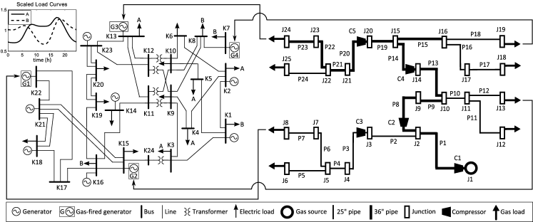
Figure 3: Schematic of integrated electric and gas test networks (reproduced from [41]). IEEE RTS96 One Area 24 node power system (left) coupled to the 24 pipe benchmark gas pipeline (right) through gas-fired generators (G1 to G4). Electric loads marked with A or B are scaled by the time-varying load curves in the inset plot at top left. Electric buses (K1 to K24), gas pipes (P1 to P24), pipe junctions (J1 to J25), and gas compressors (C1 to C5) are indicated.

Formulation 2: Chance-Constrained Power + Robust Gas: Our last formulation is the proposed method (42), which includes chance constraints to account for uncertainty in power system operation scheduling, as well as the three scenarios required to guarantee feasibility of the gas pipeline system.

VII-B Test Case and Implementation

We synthesize a case study based on the data from our previous work [41], [191]. We investigate different loading conditions, with mean electricity demand equal to 90% of the maximum load level, scaled using the profiles in Figure 3. The uncertainty in the electric power demand $\omega$ is modeled as a multivariate normal distribution with zero mean and variance equal to 3.5% of the load, i.e., $0.035\cdot h(t)$. The acceptable violation probabilities are set to $\varepsilon=0.1$ for the line constraints and $\varepsilon=0.01$ for the generator constraints. The ramp rates for the generators are adapted from a previous study [192].

In the gas network, the demand profiles for the gas-fired generators are derived from the scheduled power generation and the reserve activation, as described in Section VI. All other gas pipeline loads are set to constant values. There are four nodes with gas-fired generators G1-G4, as seen in Figure 3. Each of those generation nodes includes several generation units. The heat rate parameters in (40) with $c_{0}=0$, and $c_{1}=10$ mmbtu/MWh for the peaking plant (6 generation units in G1 and 5 generation units in G2), and $c_{1}=15$ mmbtu/MWh for combined cycle plants (1 generation unit in G2, and 3 generation units in both G3 and G4).

In alignment with standard power system operating practices, we solve the system over a time horizon of 24 hours. However, because the intra-day generation dispatch is not necessarily time periodic (particularly not when considering the activation of reserves), we extend the time horizon of the computation to 30 hours and enforce that the system is time-periodic over this extended horizon. This allows us to compute a schedule for the non-time-periodic trajectories. The objective function only considers the first 24 hours. While the original test system only includes loading scenarios for each hour, we need smaller time discretization to accurately capture the transient dynamics of the gas flow. For the optimization problem, we extend the data set to have time steps of 30 minutes, while the simulations assume 10 minute time steps. The load at each time step is obtained by interpolating between the load at each hour.

VII-C Framework for Evaluation

We evaluate the performance of our method using the following workflow.

1. Choose load and uncertainty levels for the test case.

2. Compute schedule solutions to Formulations 0, 1 and 2 to obtain a schedule for the power and gas networks.

3. Run a Monte Carlo simulation to assess the system performance.

We elaborate more on the Monte Carlo simulation and evaluation metrics that we use to assess the performance.

VII-C1 Monte Carlo simulation

To obtain statistics of system performance, such as constraint violations, we run Monte Carlo simulations. As previous studies have investigated the impact of renewable energy fluctuations on power system constraint violations in detail [131, 134, 138], the present study focuses on constraint violations in the natural gas system and their impact in terms of load shed by the power system. In each simulation, we generate a time-series for the uncertain electric load time series by drawing a new realization of the deviation $\omega$ every 10 minutes. We then solve the DC power flow (12) for each hour, where we assume that the generators are adjusted to balance load according to the reserve activation policy (2). The generation by gas-fired power plants is translated to a real-time gas withdrawal $\mathbf{\tilde{d}}^{\mathrm{nom}}$ using the generator heat rate (40). We then formulate an initial boundary value problem (IBVP) for the natural gas network. As initial conditions, we utilize the first timestep from the nominal gas flow trajectory obtained from the optimization problem solution. The compression ratios $\bm{\alpha}$ are also obtained from the optimization problem solution. Given these parameters, the IBVP has a unique solution obtained through a simulation using a DAE discretization [163].

VII-C2 Pressure Bound Violations

The IBVP simulation provides us with the density trajectories for each node in the pipeline network. Based on these trajectories, we calculate the maximum pressure constraint violation,

$$\!\!\!\!V_{\mathbf{p}}^{\max}\!=\!\max_{t}(\pi^{\min}-\pi(t))_{+}$$ (45)

and the maximum pressure constraint violation $L_{2}$ norm

$$||V_{\mathbf{p}}||_{2}\!=\!\frac{1}{N_{h}}\sum_{t\in\mathcal{T}}\sum_{i\in\mathcal{V}}(\pi^{\min}-\pi(t))_{+}^{2}$$ (46)

where $(x)_{+}=x$ if $x\geq 0$ and $(x)_{+}\equiv 0$ if $x<0$. Note that we only examine violations of the lower pressure bounds $\pi^{\min}$ in the simulation, because by construction compressor control is bounded at a maximum discharge pressure.

VII-C3 Generator curtailment analysis

To avoid violations of the lower pressure limits, gas supply to gas-fired power plants may be curtailed, leading to a reduction in electric power output. This represents a shortfall in generation capacity, which must be covered by other electric generation resources in an ad-hoc manner, and which increases operational risk. To assess this risk, we quantify the impact of reduced gas supply in terms of generation capacity curtailment.

For each scenario $\omega(t)$, the desired gas consumptions of the gas-fired power plants are given by

$$d_{\mathrm{desired}}(t)=q_{\mathrm{heat}}(\tilde{p}(t)),$$

where $\tilde{p}(t)$ is determined by the generation control policy (2). The expected amount of curtailments is characterized by solving an adapted version of the deterministic optimal gas flow scheduling (37). This problem maximizes the gas consumptions $\mathbf{d}$ of the generators, with the upper bound set equal to the desired withdrawals $d^{\max}=d_{\mathrm{desired}}(t)$ and the compressor schedule $\alpha(t)$ fixed to the solution obtained from Formulation 0, 1 or 2, respectively. The optimized gas delivery, which may be below $d_{\mathrm{desired}}(t)$, is then translated back through the heat rate to an adapted generation schedule. This schedule is used to compute the generation capacity curtailment $\Delta p$,

$$\Delta p=\frac{1}{N_{h}}\sum_{t\in\mathcal{T}}\sum_{j\in\mathcal{G}_{\textrm{gas}}}(\tilde{p}_{j}(t)-q_{\mathrm{heat}}^{-1}(\mathbf{d}_{j}(t))).$$ (47)

Here, $N_{h}$ is the number of time steps per hour and $\mathcal{G}_{\textrm{gas}}$ represents the set of gas-fired generators. The units of the generation capacity curtailment is [MWh], which represents the total energy curtailment (across all gas-fired generators) across the entire day.

VIII Case Study: Computational Results

With the above case study set up, we compare the performance of our proposed method (Formulation 2) against the two other formulations that do not account for the impact of reserve activation on the gas pipeline network, and assumes either predetermined reserve capacities (Formulation 0) or reserve capacities scheduled using the chance-constrained optimal power flow (Formulation 1). We focus our attention on constraint violations in the natural gas network, because previous work has analyzed the performance of similar chance-constrained optimal power flow formulations [134, 131, 138].

VIII-A Comparison of Cost and Schedules

We first analyze the cost and the schedules for the three formulations. The objective function values, as well as the scheduled generation and reserve capacities from gas generators are shown in Table I. Note that the cost of energy used by the compressors is several orders of magnitude smaller than the cost of electricity generation. The generation and compression cost is almost the same for Formulation 0 and 1, while Formulation 2 has approximately 1% higher cost. This modest increase in cost arises from the extra constraints that are included to guarantee robustness. Note also that all three formulations schedule a similar amount of generation from the gas-fired generators, while Formulation 0 allocates to them a lower amount of reserve capacity. This may be due to the fact that Formulation 0 does not account for the impact of the reserves on power system constraints such as line flow limits.

TABLE I: Scheduling Solutions

Formulation	Power	Compression	Nominal Gas	Reserve Gas
(90% load level)	Cost $J_{P}$	Cost $J_{C}$	Generation $\mathbf{\bar{p}}$	Capacity $\mathbf{r}$
	[$M]	[$]	[MW]	[MW]
Formulation 0	4.88	401.5	17482.1	2291.0
Formulation 1	4.89	401.4	17482.0	2683.0
Formulation 2	4.94	425.5	17482.0	2683.0

While the total amount of generation and reserves scheduled from gas-fired generators is similar for all formulations, the allocation is not homogeneous. Relative to the other two formulations, Formulation 2 schedules less generation from G2 and more generation from G3. Furthermore, generator G2 also provides less reserves in Formulation 2, while G1 and G4 provide more. To support the higher gas withdrawals at node J24 (which supplies G3) and more variable withdrawals at node J19 (which supplies G4), compressor C4 has a higher compression ratio. This demonstrates how the needs of the electric grid can impact gas pipelines.

VIII-B Pressure Violations and Generator Capacity Curtailment

To assess the quality of solutions to Formulations 0, 1 and 2, we calculate the maximum pressure violation (45), the $L_{2}$ norm of the pressure violation (46), and the corresponding generation capacity curtailment (47) for each scenario. The average values of the pressure violations and curtailment across all scenarios are shown in Table II, while Figure 4 shows the probability distribution derived from the Monte Carlo samples.

TABLE II: Statistics from Monte Carlo Simulation

Formulation	Mean Max.	Mean Integrated	Mean Load
(90% load level)	Pressure Viol. [psi]	Pressure Viol. [psi-hrs]	Shed [MWh]
Formulation 0	2.61	5.69	81.9
Formulation 1	3.67	7.32	115.9
Formulation 2	0.00	0.00	0.00

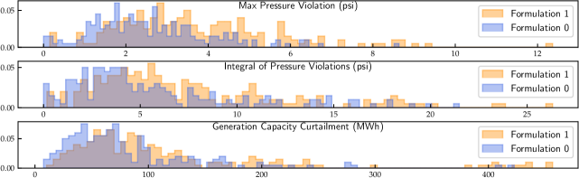
Figure 4: Empirical probability distribution of the pressure violations and generator capacity curtailment. Monte Carlo results that quantify how insufficient gas packed in the pipeline lead to curtailment of generation. Top: Maximum violation of minimum pressure constraints as given by Eq. (45). Center: $L_{2}$ norm of pressure violation over the simulation interval in psi-hours, given by Eq. (46). Bottom: Expected total load shed (MWh) per day, computed from solving Problem (37) for scenarios with pressure violations. Formulation 2 is not included, because it does not result in any violations or curtailments.

From Table II, we observe that our proposed joint scheduling and uncertainty management method (Formulation 2) does not lead to violations or generator capacity curtailments in any of the scenarios. This is as expected, because the proposed formulation guarantees gas pipeline network feasibility for provision of gas for both energy and reserves. The other two formulations, which do not consider the linepack required to guarantee reserves, lead to minimum pressure constraint violations and generator capacity curtailments. The maximum amount of pressure violations is 2.6 psi (Formulation 0) and 3.7 psi (Formulation 1). Over the course of the day, the pressure violations result in an average curtailment in generation from gas-fired power plants of 81.9 MWh and 115.9 MWh per day for Formulations 0 and 1, respectively. While we do not explicitly model the impact of this shortfall in energy on the electric system, it clearly impacts the system operator’s ability to maintain safe operations.

While the above numbers give an indication of the average performance in terms of pressure violations, we analyze the scenario corresponding to the maximum gas withdrawals. For this scenario, we plot pressure trajectories for each node in the system in Figure 5. For the proposed method (Formulation 2), all pressure trajectories stay within the the limits (area shaded in grey). In Formulations 0 and 1, the pressure trajectories start from the same feasible point, then rapidly lose feasibility. Towards the end of the day, a majority of the nodes (with pressure trajectories marked in red) are below the lower pressure bounds. We observe that the pressure violations in this scenario are much more significant than the average violations, with some pressures dropping more than 50 psi below the limit.

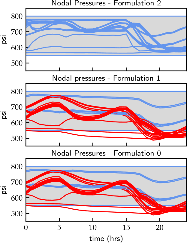
Figure 5: Pressure trajectories for the maximum gas withdrawal scenario. We simulate the case with maximum gas withdrawal (corresponding to full activation of reserves) for the solutions corresponding to Formulation 2 (top), Formulation 1 (middle) and Formulation 0 (bottom). The grey area represent the range of feasible pressures. The lines represent the pressure trajectories at each node, including both feasible (blue) and infeasible (red) trajectories.

VIII-C Robustness of the Joint Uncertainty Management

To demonstrate some characteristics of the robust gas system formulation, we investigate the pressure at one particular node (gas node 19, which is connected to electric node 7). Figure 6 shows the pressure trajectories corresponding to the nominal, maximum and minimum withdrawal cases from the joint scheduling and uncertainty management problem (plotted in yellow), as well as the pressure trajectories from the Monte Carlo simulations (plotted in blue). All the simulated trajectories start from the same state as the nominal pressure trajectory. We observe that the Monte Carlo pressure trajectories initially follow the nominal trajectory, but then slowly spread out over a larger range. However, after approximately 12 hours, the spread seems to stabilize and not increase further. Furthermore, the simulated trajectories remain far away from the yellow lines representing the pressure trajectories of the minimum and maximum withdrawal cases.

The behavior of the Monte Carlo trajectories can be explained by considering the distribution of the reserve activation. The deviations in the power loads $\omega(t)$ are modeled as a multivariate normal distribution, with no spatial or temporal correlation. This implies that the reserve activation, which is based on the total power imbalance $\Omega(t)$, and the corresponding gas consumptions are also normally distributed, with independent values at each time step. Over time, the gas withdrawals required for reserve activation hence average to zero. Therefore, the solution mostly adjusts when generators withdraw gas, as opposed to how much gas is withdrawn in total (although there are of course differences). Consequently, the pressure trajectories do not deviate very far from the nominal. If we instead had a consistent activation of the upward or downward reserves, we expect a much larger spread in the observed pressure trajectories.

Finally, we would like to note that our formulation is not only robust to variations in the gas withdrawals, but also robust with respect to the initial conditions. Although we chose to start all Monte Carlo simulations from the system state corresponding to the nominal gas withdrawals, any initial condition with pressures in the range between (and including) the yellow lines would be robustly feasible to variations in the gas withdrawals. This can be useful for operational planning purposes, when the exact operating point at the beginning of the next day is not yet known.

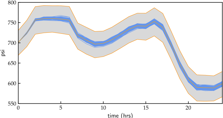
Figure 6: Robust pressure trajectories for node 19. We show the pressure trajectories for gas node 19 (power node 7). The yellow lines are the nominal, upper and lower pressure profiles obtained from Formulation 2, corresponding to the nominal, minimum and maximum withdrawal levels $\textbf{d}^{\textrm{nom}},\textbf{d}^{\min}$ and $\textbf{d}^{\max}$. The area between them is shaded in grey. The blue lines are pressure trajectories from the Monte Carlo simulation, which start at a nominal initial state, and diverge depending on reserve activation in the power system.

IX Conclusions

This paper reviews the emerging trends in the energy sector that motivate integrated optimization and coordination mechanisms for gas pipelines and the electric grid, with a particular focus on managing intra-day uncertainty. One of the open challenges identified in the literature review is a method for joint optimization of generation, allocation of reserves, and gas pipeline flows under consideration of uncertainty and transient gas pipeline flows. To tackle this challenge, we propose a framework that defines the interface between the electric and gas networks as a nominal schedule, as well as upper and lower bounds on the gas consumed by gas-fired power plants. Our proposed formulation builds on established approaches for chance-constrained optimal power flow and new ideas for robust optimization of transient natural gas flow. The proposed approach results in a numerically tractable optimization problem that achieves integrated scheduling with probabilistic and robust safety guarantees. In our case study, we benchmark our proposed framework against other joint optimization formulations in a case study with interacting test networks. Through Monte Carlo simulations, we verify the robust guarantees of our approach and demonstrate that such guarantees are essential to ensure operating reliability of both gas pipelines and power grids with high renewable contributions.

Line Roald is an Assistant Professor and Grainger Institute Fellow in the Department of Electrical and Computer Engineering in University of Wisconsin–Madison. She received her Ph.D. degree in Electrical Engineering (2016) and M.Sc. and B.Sc. degrees in Mechanical Engineering from ETH Zurich, Zurich, Switzerland. She was a postdoctoral research fellow with the Center of Non-Linear Studies at Los Alamos National Laboratory. Her research interests focus on modeling and optimization of energy systems, with a particular focus on managing uncertainty and risk from renewable energy variability and component failures.

Kaarthik Sundar received the Ph.D. degree in mechanical engineering from Texas A&M University, College Station, TX, USA, in 2016. He is currently a Research Scientist in the Information Systems and Modeling Division at Los Alamos National Laboratory, Los Alamos, NM, USA. His research interests include problems pertaining to vehicle routing, path planning, and control for unmanned/autonomous systems; numerical optimal control, estimation, and large-scale optimization problems in power and gas networks; combinatorial optimization; and global optimization for mixed-integer nonlinear programs.

Anatoly Zlotnik (M10) is a staff scientist in the Applied Mathematics and Plasma Physics group of the Theoretical Division at Los Alamos National Laboratory, where he was previously a postdoctoral associate at the Center for Nonlinear Studies. Before joining LANL in 2014, he obtained a Ph.D. in systems science and mathematics from Washington University in St. Louis, Missouri, an M.S. in applied mathematics from the University of Nebraska – Lincoln, and B.S. and M.S. degrees in systems and control engineering from Case Western Reserve University in Cleveland, Ohio. His research focus is on computational methods for optimal control of large-scale nonlinear dynamic systems.

Sidhant Misra Sidhant Misra received the Ph.D. degree in electrical engineering and computer science from the Massachusetts Institute of Technology, Cambridge, MA, USA, in 2014. He is currently a Research Scientist in the theory division and the Advanced Network Science Initiative at the Los Alamos National Laboratory, Los Alamos, NM, USA. His research interests lie at the intersection of machine learning and optimization with applications in network structure identification, and planning and operations of energy networks.

Göran Andersson (M’86, SM’91, F’97) obtained his M.S. (1975) and Ph.D. (1980) degrees from the University of Lund, Sweden. In 1980 he joined ASEA’s, now ABB’s, HVDC division in Ludvika, Sweden, and in 1986 he was appointed professor in electric power systems at KTH (Royal Institute of Technology), Stockholm, Sweden. In 2000 - 2016 he was full professor in electric power systems at ETH Zürich (Swiss Federal Institute of Technology). His research interests include power system dynamics, control and operation, power markets, and future energy systems. Göran Andersson is Fellow of the Royal Swedish Academy of Sciences, the Royal Swedish Academy of Engineering Sciences, the Swiss Academy of Engineering Sciences, and foreign member of the US National Academy of Engineering. He was the recipient of the 2007 IEEE PES Outstanding Power Educator Award, the 2010 George Montefiore International Award, and the 2016 IEEE PES Prabha S. Kundur Power System Dynamics and Control Award.

References

- [1] International Energy Agency. World energy outlook. Technical report, International Energy Agency, Paris, 2019.
- [2] J. Bistline. Natural gas, uncertainty, and climate policy in the US electric power sector. Energy Policy, 74:433–442, November 2014.
- [3] R. Domínguez, A. J. Conejo, and M. Carrión. Toward Fully Renewable Electric Energy Systems. IEEE Transactions on Power Systems, 30:316–326, January 2015.
- [4] R. Levitan, S. Wilmer, and R. Carlson. Pipeline to reliability: Unraveling gas and electric interdependencies across the eastern interconnection. Power and Energy Magazine, IEEE, 12(6):78–88, 2014.
- [5] K. W. Costello. Exploiting the Abundance of US Shale Gas: Overcoming Obstacles to Fuel Switching and Expanding the Gas Distribution System. Energy Law Journal, 34:541, 2013.
- [6] J. Bistline. Electric sector capacity planning under uncertainty: Climate policy and natural gas in the US. Energy Econ., 51:236–251, 2015.
- [7] E. J. Moniz et al. The future of natural gas. Cambridge, MA: Massachusetts Institute of Technology, 2011.
- [8] J. Logan, A. Lopez, et al. Natural gas scenarios in the US power sector. Energy Economics, 40:183–195, 2013.
- [9] R. F. Aguilera. Revisiting the role of natural gas as a transition fuel. Mineral Economics, pages 1–8, 2019.
- [10] Sobhan Badakhshan, Neda Hajibandeh, Miadreza Shafie-khah, and João PS Catalão. Impact of solar energy on the integrated operation of electricity-gas grids. Energy, 183:844 – 853, 2019.
- [11] E. Hittinger, J. F. Whitacre, and J. Apt. Compensating for wind variability using co-located natural gas generation and energy storage. Energy Systems, 1:417–439, December 2010.
- [12] M. Chertkov, S. Backhaus, and V. Lebedev. Cascading of fluctuations in interdependent energy infrastructures: Gas-grid coupling. Applied Energy, 160:541 – 551, 2015.
- [13] R. Rubio, D. Ojeda-Esteybar, O. Ano, and A. Vargas. Integrated natural gas and electricity market: A survey of the state of the art in operation planning and market issues. In IEEE PES Transmission and Distribution: Latin America, pages 1–8, 2008.
- [14] M Chertkov, M Fisher, S Backhaus, R Bent, and S Misra. Pressure Fluctuations in Natural Gas Networks caused by Gas-Electric Coupling. In 48th Hawaii Internatl. Conf. on System Sci. IEEE, 2015.
- [15] M. Babula and K. Petak. The cold truth: Managing gas-electric integration: The ISO New England experience. IEEE Power & Energy Mag., 12(6):20–28, 2014.
- [16] T. Pugh and J. P. Blackford. Implications of greater reliance on natural gas for electric generation, 2010.
- [17] M. Shahidehpour and Z. Li. White paper: Long-term electric and natural gas infrastructure requirements. Technical report, Illinois Institute of Technology, 2014.
- [18] ICF International. Assessment of new england’s natural gas pipeline capacity to satisfy short and near-term electric generation needs. Technical report, ISO New England, 2012.
- [19] A. J. Wood, B. F. Wollenberg, and G. B. Sheble. Power Generation, Operation and Control, 3rd Edition. Wiley, 2013.
- [20] R. G. Carter and H. H. Rachford Jr. Optimizing line-pack management to hedge against future load uncertainty. In PSIG annual meeting. Pipeline Simulation Interest Group, 2003.
- [21] M. Vuffray, S. Misra, and M. Chertkov. Monotonicity of dissipative flow networks renders robust maximum profit problem tractable: General analysis and application to natural gas flows. In 54th IEEE Conf. on Decision and Control, pages 4571–4578. IEEE, 2015.
- [22] S. Misra, M. Vuffray, A. Zlotnik, and M. Chertkov. Monotone order properties for control of nonlinear parabolic pde on graphs. In Proc. 22nd International Symposium on Mathematical Theory of Networks and Systems, arXiv preprint arXiv:1601.05102, 2016.
- [23] S. Misra, M. Vuffray, and A. Zlotnik. Monotonicity properties of physical network flows and application to robust optimal allocation. Submitted to the Proceedings of the IEEE, 2020.
- [24] Black and Veatch. New england natural gas infrastructure and electric generation: Constraints and solutions. Technical report, The New England States Committee on Electricity, 2013.
- [25] MIT Energy Institute. Growing concerns, possible solutions: The interdependency of natural gas and electricity systems. Technical report, Massachusets Institute of Technology, 2013.
- [26] R. Carter, A. V. Zlotnik, S. Backhaus, M. Chertkov, A. Daniels, A. Hollis, and A. Giacomoni. Impact of regulatory change to coordinate gas pipelines and power systems. In PSIG Annual Meeting, page 1612. Pipeline Simulation Interest Group, 2016.
- [27] P. Myles, K. Labarbara, and C. E. Logan. Ensuring reliable natural gas-fired power generation with fuel contracts and storage. Technical report, NETL, 2017.
- [28] E. Litvinov. Design and operation of the locational marginal prices-based electricity markets. Generation, Transmission Distribution, IET, 4(2):315–323, February 2010.
- [29] Forward Market Operations. Energy & Ancillary Services Market Operations, M-11 Rev. 75. Technical report, PJM, 2015.
- [30] ISO New England. ISO New England Manual for Market Operations, M-11 Rev. 49. Technical report, ISONE, 2014.
- [31] N. Wang and G. Mogi. Deregulation, market competition, and innovation of utilities: Evidence from japanese electric sector. Energy Policy, 111:403–413, 2017.
- [32] G. Razeghi, B. Shaffer, and S. Samuelsen. Impact of electricity deregulation in the state of california. Energy Policy, 103:105–115, 2017.
- [33] N. M. Lindsay and A. K. Parvathy. Power system reliability assessment in a complex restructured power system. International Journal of Electrical & Computer Engineering (2088-8708), 9, 2019.
- [34] F. Feijoo, G. C. Iyer, C. Avraam, S. A. Siddiqui, L. E. Clarke, S. Sankaranarayanan, M. T. Binsted, P. L. Patel, N. C. Prates, E. Torres-Alfaro, et al. The future of natural gas infrastructure development in the United States. Applied energy, 228:149–166, 2018.
- [35] M. E. Oliver. Economies of scale and scope in expansion of the U.S. natural gas pipeline network. Energy Economics, 52:265–276, 2015.
- [36] T. Koch, B. Hiller, M. Pfetsch, and L. Schewe. Evaluating gas network capacities. SIAM, 2015.
- [37] A. V. Zlotnik, A. M. Rudkevich, et al. Economic optimization of intra-day gas pipeline flow schedules using transient flow models. In PSIG Annual Meeting. Pipeline Simulation Interest Group, 2017.
- [38] A. M. Rudkevich and A. Zlotnik. Locational marginal pricing of natural gas subject to engineering constraints. In 50th Hawaii International Conference onSystem Sciences (HICSS). IEEE, 2017.
- [39] N. N. Novitsky, A. V. Alekseev, et al. Multilevel modeling and optimization of large-scale pipeline systems operation. Energy, 184:151–164, 2019.
- [40] B. Zhao, A. Zlotnik, A. J. Conejo, R. Sioshansi, and A. M. Rudkevich. Shadow price-based co-ordination of natural gas and electric power systems. IEEE Trans. Power Sys., 34(3):1942–1954, 2018.
- [41] A Zlotnik, L. Roald, S. Backhaus, M. Chertkov, and G. Andersson. Coordinated Scheduling for Interdependent Electric Power and Natural Gas Infrastructures. IEEE Trans. Power Sys., 32(1):600 – 610, 2017.
- [42] E. Guelpa, A. Bischi, V. Verda, M. Chertkov, and H. Lund. Towards future infrastructures for sustainable multi-energy systems: A review. Energy, 2019.
- [43] J. Yu, M. Ma, and L. Guo. Reliability evaluation of integrated electrical and natural-gas system with power-to-gas. In Proceedings of the CSEE, volume 38, pages 708–715, 2018.
- [44] G. Guandalini, S. Campanari, and M. C. Romano. Power-to-gas plants and gas turbines for improved wind energy dispatchability: Energy and economic assessment. Applied Energy, 147:117–130, 2015.
- [45] S. Clegg and P. Mancarella. Storing renewables in the gas network: modelling of power-to-gas seasonal storage flexibility in low-carbon power systems. IET Generation, Transmission & Distribution, 10(3):566–575, 2016.
- [46] S. An, Q. Li, and T. W. Gedra. Natural gas and electricity optimal power flow. In Transmission and Distribution Conference and Exposition, 2003 IEEE PES, volume 1, pages 138–143. IEEE, 2003.
- [47] M. Geidl and G. Andersson. Optimal power flow of multiple energy carriers. IEEE Trans. Power Sys., 22(1):145–155, 2007.
- [48] C. Unsihuay, J. W. M. Lima, and A. C. Z. De Souza. Modeling the integrated natural gas and electricity optimal power flow. In IEEE Power Engineering Society General Meeting, pages 1–7. IEEE, 2007.
- [49] T. Li, M. Eremia, and Mohammad Shahidehpour. Interdependency of natural gas network and power system security. Power Systems, IEEE Transactions on, 23(4):1817–1824, 2008.
- [50] C. Liu, M. Shahidehpour, Y. Fu, and Z. Li. Security-constrained unit commitment with natural gas transmission constraints. IEEE Transactions on Power Systems, 24(3):1523–1536, 2009.
- [51] C. M. Correa-Posada and P. Sánchez. Security-constrained optimal power and natural-gas flow. IEEE Transactions on Power Systems, 29(4):1780–1787, 2014.
- [52] L. Wu and M. Shahidehpour. Optimal coordination of stochastic hydro and natural gas supplies in midterm operation of power systems. Generation, Transmission & Distribution, 5(5):577–587, 2011.
- [53] C. Liu, M. Shahidehpour, and J. Wang. Application of augmented lagrangian relaxation to coordinated scheduling of interdependent hydrothermal power and natural gas systems. Generation, Transmission & Distribution, 4(12):1314–1325, 2010.
- [54] C. A. Saldarriaga, R. A. Hincapie, and H. Salazar. A holistic approach for planning natural gas and electricity distribution networks. IEEE Transactions on Power Systems, 28(4):4052–4063, 2013.
- [55] C. Liu, M. Shahidehpour, and J. Wang. Coordinated scheduling of electricity and natural gas infrastructures with a transient model for natural gas flow. Chaos, 21(2):025102, 2011.
- [56] Y. Zhou, C. Gu, H. Wu, and Y. Song. An Equivalent Model of Gas Networks for Dynamic Analysis of Gas-Electricity Systems. IEEE Trans. Power Sys., 32:4255–4264, 2017.
- [57] S. Chen, A. J. Conejo, R. Sioshansi, and Z. Wei. Unit commitment with an enhanced natural gas-flow model. IEEE Trans. Power Sys., 2019.
- [58] Y.-Q. Bao, M. Wu, X. Zhou, and X. Tang. Piecewise Linear Approximation of Gas Flow Function for the Optimization of Integrated Electricity and Natural Gas System. IEEE Access, 7:91819–91826, 2019.
- [59] A. Schwele, C. Ordoudis, J. Kazempour, and P. Pinson. Coordination of power and natural gas systems: Convexification approaches for linepack modeling. In 13th IEEE PES PowerTech Conference, 2019.
- [60] S. Badakhshan et al. Security-constrained unit commitment with natural gas pipeline transient constraints. IEEE Trans. Smart Grid, 2019.
- [61] Chengcheng Shao, Mohammad Shahidehpour, Xifan Wang, Xiuli Wang, and Biyang Wang. Integrated Planning of Electricity and Natural Gas Transportation Systems for Enhancing the Power Grid Resilience. IEEE Trans. Power Sys., 32:4418–4429, 2017.
- [62] B. Zhao, A. J. Conejo, and R. Sioshansi. Using Electrical Energy Storage to Mitigate Natural Gas-Supply Shortages. IEEE Trans. Power Sys., 2019. in press.
- [63] C. O’Malley, L. Roald, D. Kourounis, O. Schenk, and G. Hug. Security assessment in gas-electric networks. In 2018 Power Systems Computation Conference (PSCC), pages 1–7. IEEE, 2018.
- [64] C. He, L. Wu, T. Liu, and Z. Bie. Robust Co-optimization Planning of Interdependent Electricity and Natural Gas Systems with a Joint and Probabilistic Reliability Criterion. IEEE Trans. Power Sys., 33:2140–2154, 2018.
- [65] M. Jamei, E. Schweitzer, A. Scaglione, and K. W. Hedman. Gas and electric grid unit commitment with coordinated n-1 generator contingency analysis. In 2018 Power Systems Computation Conference (PSCC), pages 1–7. IEEE, 2018.
- [66] Y. Hu, Z. Bie, T. Ding, and Y. Lin. An NSGA-II based multi-objective optimization for combined gas and electricity network expansion planning. Applied Energy, 167:280–293, 2016.
- [67] Q. Zeng, B. Zhang, J. Fang, and Z. Chen. A bi-level programming for multistage co-expansion planning of the integrated gas and electricity system. Applied Energy, 200:192–203, 2017.
- [68] C. Borraz-Sanchez, R. Bent, S. Backhaus, S. Blumsack, H. Hijazi, and P. Van Hentenryck. Convex optimization for joint expansion planning of natural gas and power systems. In 2016 49th Hawaii International Conference on System Sciences (HICSS), pages 2536–2545. IEEE, 2016.
- [69] B. Zhao, A. J. Conejo, and R. Sioshansi. Coordinated expansion planning of natural gas and electric power systems. IEEE Transactions on Power Systems, 33(3):3064–3075, 2018.
- [70] D. Wang, J. Qiu, et al. Coordinated expansion co-planning of integrated gas and power systems. Journal of Modern Power Systems and Clean Energy, 5:314–325, 2017.
- [71] J. Qiu, H. Yang, et al. A Linear Programming Approach to Expansion Co-Planning in Gas and Electricity Markets. IEEE Trans. Power Sys., 31:3594–3606, 2016.
- [72] F. Barati, H. Seifi, et al. Multi-Period Integrated Framework of Generation, Transmission, and Natural Gas Grid Expansion Planning for Large-Scale Systems. IEEE Trans. Power Sys., 30:2527–2537, 2015.
- [73] J. Jalving, S. Abhyankar, K. Kim, M. Hereld, and V. M. Zavala. A graph-based computational framework for simulation and optimisation of coupled infrastructure networks. IET Generation, Transmission & Distribution, 11(12):3163–3176, 2017.
- [74] K. Pambour, R. Sopgwi, B.-M. Hodge, and C. Brancucci. The value of day-ahead coordination of power and natural gas network operations. Energies, 11(7):1628, 2018.
- [75] S. B. Dokic and N. L. Rajakovic. Security modelling of integrated gas and electrical power systems by analyzing critical situations and potentials for performance optimization. Energy, 184:141–150, 2019.
- [76] A. Rudkevich, A. Zlotnik, P. Ruiz, E. Goldis, A. Beylin, R. Hornby, R. Tabors, S. Backhaus, M. Caramanis, and R. Philbrick. Market based intraday coordination of electric and natural gas system operation. In Proceedings of the 51st Hawaii International Conference on System Sciences, 2018.
- [77] A. Zlotnik, K. Sundar, A. M. Rudkevich, R. Tabors, and X. Li. Pipeline transient optimization for a gas-electric coordination decision support system. In PSIG Annual Meeting. Pipeline Simulation Interest Group, 2019.
- [78] S. Clegg and P. Mancarella. Integrated electrical and gas network flexibility assessment in low-carbon multi-energy systems. IEEE Transactions on Sustainable Energy, 7(2):718–731, 2015.
- [79] A. Antenucci and G. Sansavini. Gas-constrained secure reserve allocation with large renewable penetration. IEEE Transactions on Sustainable Energy, 9(2):685–694, 2017.
- [80] Z. Yang, C. Gao, and M. Zhao. Coordination of integrated natural gas and electrical systems in day-ahead scheduling considering a novel flexible energy-use mechanism. Energy Conv. and Management, 196:117–126, 2019.
- [81] S. Chen, A. J. Conejo, R. Sioshansi, and Z. Wei. Equilibria in electricity and natural gas markets with strategic offers and bids. IEEE Trans. Power Sys., 2019.
- [82] C. Ordoudis, S. Delikaraoglou, P. Pinson, and J. Kazempour. Exploiting flexibility in coupled electricity and natural gas markets: A price-based approach. In 2017 IEEE Manchester PowerTech, pages 1–6, 2017.
- [83] C. O’Malley, S. Delikaraoglou, L. Roald, and G. Hug. Natural gas system dispatch accounting for electricity side flexibility. Electric Power Systems Research, 178:106038, 2020.
- [84] Y. Jiang, J. Xu, et al. Coordinated operation of gas-electricity integrated distribution system with multi-CCHP and distributed renewable energy sources. Applied energy, 211:237–248, 2018.
- [85] Z. Chen, Y. Zhang, et al. Coordinated optimal dispatch and market equilibrium of integrated electric power and natural gas networks with P2G embedded. J. Mod. Power Sys. & Clean Energy, 6(3):495–508, 2018.
- [86] M. Sukharev and O. Kochueva. Phenomenological study of the dynamics of pressure distribution in a gas flow in a long-distance pipeline. In E3S Web of Confs., volume 102. EDP Sciences, 2019.
- [87] M. Sukharev and V. Kulik. The impact of information uncertainty on the problems of medium-and long-term planning of the operation modes of gas transport systems. Energy, 2017.
- [88] Assessment of energy storage systems suitable for use by electric utilities. Technical Report EPRI-EM-264, Electric Power Research Institute, Palo Alto, CA, USA, 1976.
- [89] National Grid. Webinar on proposed changes to national grid’s planning assumptions / approaches. Technical report, Gas Transmission Planning Code Webinar, July 2017.
- [90] A. Zlotnik, M. Chertkov, and S. Backhaus. Optimal control of transient flow in natural gas networks. In 54th IEEE Conference on Decision and Control, pages 4563–4570, Osaka, Japan, 2015.
- [91] S. Chen, Z. Wei, G. Sun, K. W. Cheung, and Y. Sun. Multi-linear probabilistic energy flow analysis of integrated electrical and natural-gas systems. IEEE Transactions on Power Systems, 32(3):1970–1979, 2017.
- [92] D. Hu and S. M. Ryan. Stochastic vs. deterministic scheduling of a combined natural gas and power system with uncertain wind energy. Internatl. J. Electrical Power & Energy Sys., 108:303–313, 2019.
- [93] M. Rayati, H. Goodarzi, and A. M. Ranjbar. Optimal bidding strategy of coordinated wind power and gas turbine units in real-time market using conditional value at risk. International Transactions on Electrical Energy Systems, 29(1):e2645, 2019.
- [94] C. Ordoudis, P. Pinson, and J. M. Morales. An integrated market for electricity and natural gas systems with stochastic power producers. European Journal of Operational Research, 272(2):642–654, 2019.
- [95] C. Borraz-Sanchez. Optimization methods for pipeline transportation of natural gas. PhD thesis, Bergen Univ.(Norway), 2010.
- [96] P. Wong and R. Larson. Optimization of natural-gas pipeline systems via dynamic programming. Automatic Control, IEEE Transactions on, 13(5):475–481, 1968.
- [97] S. Misra, M. W. Fisher, S. Backhaus, R. Bent, M. Chertkov, and F. Pan. Optimal compression in natural gas networks: A geometric programming approach. IEEE Trans. on Control of Network Sys., 2(1):47–56, 2015.
- [98] R. Z. Ríos-Mercado and C. Borraz-Sánchez. Optimization problems in natural gas transportation systems: A state-of-the-art review. Applied Energy, 147:536–555, 2015.
- [99] F. Wu, H. Nagarajan, A. Zlotnik, R. Sioshansi, and A. M. Rudkevich. Adaptive convex relaxations for gas pipeline network optimization. In 2017 American Control Conference (ACC), pages 4710–4716. IEEE, 2017.
- [100] M. Steinbach. On pde solution in transient optimization of gas networks. Journal of computational and applied mathematics, 203(2):345–361, 2007.
- [101] M. Abbaspour, P. Krishnaswami, and K.S. Chapman. Transient optimization in natural gas compressor stations for linepack operation. Journal of Energy Resources Technology, 129(4):314, 2007.
- [102] H. H. Rachford Jr., R. G. Carter, and T. F. Dupont. Using optimization in transient gas transmission. In PSIG Annual Meeting. Pipeline Simulation Interest Group, 2009.
- [103] A. Gopalakrishnan and L. T. Biegler. Economic nonlinear model predictive control for periodic optimal operation of gas pipeline networks. Computers & Chemical Engineering, 52:90–99, 2013.
- [104] V. Zavala. Stochastic optimal control model for natural gas networks. Computers & Chemical Engineering, 64:103–113, 2014.
- [105] M. Gugat, G. Leugering, A. Martin, M. Schmidt, M. Sirvent, and D. Wintergerst. Mip-based instantaneous control of mixed-integer pde-constrained gas transport problems. Computational Optimization and Applications, 70(1):267–294, 2018.
- [106] A. Zlotnik, K. Sundar, A. M. Rudkevich, A. Beylin, and X. Li. Optimal control for scheduling and pricing intra-day natural gas transport on pipeline networks. In 58th IEEE Conference on Decision and Control, Nice, France, 2019.
- [107] A. Rudkevich, A. Zlotnik, X. Li, P. Ruiz, A. Beylin, John G., R. Tabors, and R. Philbrick. Evaluating benefits of rolling horizon model predictive control for intraday scheduling of a natural gas pipeline market. In Proceedings of the 52nd Hawaii International Conference on System Sciences, 2019.
- [108] M. G. Sukharev, K. O. Kosova, and R. V. Popov. Mathematical and computer models for identification and optimal control of large-scale gas supply systems. Energy, 184:113–122, 2019.
- [109] C. O’Malley, D. Kourounis, G. Hug, and O. Schenk. Optimizing gas networks using adjoint gradients. arXiv preprint arXiv:1804.09601, 2018.
- [110] S. Moritz. A mixed integer approach for the transient case of gas network optimization. PhD thesis, TU Darmstadt, 2007.
- [111] H. H. Rachford and R. G. Carter. Optimizing pipeline control in transient gas flow. In PSIG annual meeting. Pipeline Simulation Interest Group, 2000.
- [112] K. Ehrhardt and M. Steinbach. Nonlinear optimization in gas networks. Springer, 2005.
- [113] A. Zlotnik, S. Dyachenko, S. Backhaus, and M. Chertkov. Model reduction and optimization of natural gas pipeline dynamics. In ASME Dynamic Systems and Control Conference, page V003T39A002, Columbus, OH, 2015.
- [114] A. Gopalakrishnan and L. T. Biegler. Economic nonlinear model predictive control for periodic optimal operation of gas pipeline networks. Computers & Chemical Engineering, 52:90–99, 2013.
- [115] M. T. Devine, J. P. Gleeson, J. Kinsella, and D. M. Ramsey. A rolling optimisation model of the uk natural gas market. Networks and Spatial Economics, 14(2):209–244, 2014.
- [116] T. W. K. Mak, P. Van Hentenryck, A. Zlotnik, H. Hijazi, and R. Bent. Efficient dynamic compressor optimization in natural gas transmission systems. In IEEE American Control Conference, pages 7484–7491, Boston, MA, 2016.
- [117] T. W. K. Mak, P. Van Hentenryck, A. Zlotnik, and R. Bent. Dynamic compressor optimization in natural gas pipeline systems. INFORMS J. on Computing, 31(1):40–65, 2019.
- [118] S. A. Dyachenko, A. Zlotnik, A. O. Korotkevich, and M. Chertkov. Operator splitting method for simulation of dynamic flows in natural gas pipeline networks. Physica D: Nonlinear Phenomena, 361:1–11, 2017.
- [119] V. Gyrya and A. Zlotnik. An explicit staggered-grid method for numerical simulation of large-scale natural gas pipeline networks. Applied Mathematical Modelling, 65:34–51, 2019.
- [120] P. Panciatici, Y. Hassaine, S. Fliscounakis, L. Platbrood, M. Ortega-Vazquez, J.L. Martinez-Ramos, and L. Wehenkel. Security management under uncertainty: From day-ahead planning to intraday operation. In IREP Symposium, pages 1–8, Buzios, Brazil, Aug 2010.
- [121] F. Capitanescu, S. Fliscounakis, P. Panciatici, and L. Wehenkel. Cautious operation planning under uncertainties. IEEE Transactions on Power Systems, 27(4):1859–1869, Nov 2012.
- [122] J. Warrington, P. J. Goulart, S. Mariethoz, and M. Morari. Policy-based reserves for power systems. IEEE Transactions on Power Systems, 28(4):4427–4437, 2013.
- [123] A. Lorca, X. A. Sun, E. Litvinov, and T. Zheng. Multistage adaptive robust optimization for the unit commitment problem. Operations Research, 64(1):32–51, 2016.
- [124] F. Bouffard and F. D. Galiana. Stochastic security for operations planning with significant wind power generation. IEEE Transactions on Power Transactions on Power, 23:306–316, May 2008.
- [125] J. M. Morales, A. J. Conejo, and J. Perez-Ruiz. Economic valuation of reserves in power systems with high penetration of wind power. IEEE Transactions on Power Systems, 24(2):900–910, May 2009.
- [126] A. Papavasiliou and S. S. Oren. Multiarea stochastic unit commitment for high wind penetration in a transmission constrained network. Operations Research, 61(3):578–592, 2013.
- [127] J. Wang, M. Shahidehpour, and Z. Li. Security-constrained unit commitment with volatile wind power generation. IEEE Trans. Power Sys., 23(3):1319–1327, 2008.
- [128] T. Tinoco De Rubira and G. Hug. Adaptive certainty-equivalent approach for optimal generator dispatch under uncertainty. In European Control Conference (ECC), Aalborg, Denmark, 2016.
- [129] U. A. Ozturk, M. Mazumdar, and B. A. Norman. A solution to the stochastic unit commitment problem using chance constrained programming. IEEE Trans. Power Sys., 19(3):1589–1598, Aug 2004.
- [130] M. Vrakopoulou, K. Margellos, J. Lygeros, and G. Andersson. A Probabilistic Framework for Reserve Scheduling and N-1 Security Assessment of Systems With High Wind Power Penetration. IEEE Transactions on Power Systems, 28(4):3885–3896, 2013.
- [131] L. Roald, F. Oldewurtel, T. Krause, and G. Andersson. Analytical reformulation of security constrained optimal power flow with probabilistic constraints. In 2013 IEEE Grenoble Conference, pages 1–6. IEEE, 2013.
- [132] C. Hamon, M. Perninge, and L. Söder. The value of using chance-constrained optimal power flows for generation re-dispatch under uncertainty with detailed security constraints. In PES Asia-Pacific Power and Energy Engineering Conference, pages 1–6. IEEE, 2013.
- [133] K. Margellos, V. Rostampour, M. Vrakopoulou, M. Prandini, G. Andersson, and J. Lygeros. Stochastic unit commitment and reserve scheduling: A tractable formulation with probabilistic certificates. In 2013 European Control Conference (ECC), pages 2513–2518. IEEE, 2013.
- [134] D. Bienstock, M. Chertkov, and S. Harnett. Chance-constrained optimal power flow: Risk-aware network control under uncertainty. Siam Review, 56(3):461–495, 2014.
- [135] T. Summers, J. Warrington, M. Morari, and J. Lygeros. Stochastic optimal power flow based on convex approximations of chance constraints. In Power Systems Computation Conference, pages 1–7. IEEE, 2014.
- [136] L Roald, S. Misra, M. Chertkov, and G. Andersson. Optimal power flow with weighted chance constraints and general policies for generation control. In 2015 IEEE 54th Annual Conference on Decision and Control (CDC), pages 6927–6933. IEEE, 2015.
- [137] M. Lubin, Y. Dvorkin, and S. Backhaus. A robust approach to chance constrained optimal power flow with renewable generation. IEEE Trans. Power Sys., 31(5):3840–3849, 2015.
- [138] L. Roald, S. Misra, T. Krause, and G. Andersson. Corrective control to handle forecast uncertainty: A chance constrained optimal power flow. IEEE Trans. Power Sys., 32(2):1626–1637, 2016.
- [139] E. Dall’Anese, K. Baker, and T. Summers. Chance-constrained AC optimal power flow for distribution systems with renewables. IEEE Trans. Power Sys., 32(5):3427–3438, 2017.
- [140] X. Geng and L. Xie. Chance-constrained unit commitment via the scenario approach, 2019.
- [141] C. Sahin, Z. Li, M. Shahidehpour, and I. Erkmen. Impact of natural gas system on risk-constrained midterm hydrothermal scheduling. IEEE Transactions on Power Systems, 26(2):520–531, 2011.
- [142] C. Sahin, M. Shahidehpour, and I. Erkmen. Generation risk assessment in volatile conditions with wind, hydro, and natural gas units. Applied Energy, 96:4–11, 2012.
- [143] I. Vos. The impact of wind power on european natural gas markets. OECD, 2012.
- [144] R. Dorsey-Palmateer. Effects of wind power intermittency on generation and emissions. The Electricity Journal, 32(3):25–30, 2019.
- [145] Z. Qiao, Q. Guo, et al. An interval gas flow analysis in natural gas and electricity coupled networks considering the uncertainty of wind power. Applied energy, 201:343–353, 2017.
- [146] J. Yang. Effect of natural gas flow dynamics in robust generation scheduling under wind uncertainty. IEEE Trans. Power Sys., 33(2):2087–2097, 2017.
- [147] J. G. Tamba, N. Essiane, et al. Forecasting natural gas: a literature survey. Internatl. J. Energy Econ. and Policy, 8(3):216–249, 2018.
- [148] B. Zhao, A. J. Conejo, and R. Sioshansi. Unit commitment under gas-supply uncertainty and gas-price variability. IEEE Transactions on Power Systems, 32(3):2394–2405, 2017.
- [149] M. Qadrdan, J. Wu, N. Jenkins, and J. Ekanayake. Operating strategies for a GB integrated gas and electricity network considering the uncertainty in wind power forecasts. IEEE Transactions on Sustainable Energy, 5(1):128–138, 2013.
- [150] A. Alabdulwahab, A. Abusorrah, X. Zhang, and M. Shahidehpour. Stochastic security-constrained scheduling of coordinated electricity and natural gas infrastructures. IEEE Systems Journal, 11(3):1674–1683, 2015.
- [151] A. Alabdulwahab, A. Abusorrah, X. Zhang, and M. Shahidehpour. Coordination of interdependent natural gas and electricity infrastructures for firming the variability of wind energy in stochastic day-ahead scheduling. IEEE Trans. on Sustainable Energy, 6(2):606–615, 2015.
- [152] L. Bai, F. Li, et al. Interval optimization based operating strategy for gas-electricity integrated energy systems considering demand response and wind uncertainty. Applied energy, 167:270–279, 2016.
- [153] C. Liu, C. Lee, and M. Shahidehpour. Look ahead robust scheduling of wind-thermal system with considering natural gas congestion. IEEE Transactions on Power Systems, 30(1):544–545, 2015.
- [154] C. He, L. Wu, T. Liu, and M. Shahidehpour. Robust co-optimization scheduling of electricity and natural gas systems via admm. IEEE Transactions on Sustainable Energy, 8(2):658–670, 2016.
- [155] L. Bai, F. Li, T. Jiang, and H. Jia. Robust scheduling for wind integrated energy systems considering gas pipeline and power transmission N–1 contingencies. IEEE Trans. on Power Systems, 32(2):1582–1584, 2016.
- [156] X. Xiao, Y. Shui, H. Gao, et al. A two-stage distributionally robust coordinated dispatch for integrated electricity and natural-gas energy systems considering uncertainty of wind power. In IOP Conference Series: Materials Science and Engineering, volume 366, page 012016. IOP Publishing, 2018.
- [157] C. He, L. Wu, et al. Co-optimization scheduling of interdependent power and gas systems with electricity and gas uncertainties. Energy, 159:1003–1015, 2018.
- [158] M. A. Mirzaei, A. Sadeghi-Yazdankhah, M. Nazari-Heris, and B. Mohammadi-ivatloo. IGDT-Based Robust Operation of Integrated Electricity and Natural Gas Networks for Managing the Variability of Wind Power. In Robust Optimal Planning and Operation of Electrical Energy Systems, pages 131–143. Springer, 2019.
- [159] C. He, T. Liu, L. Wu, and M. Shahidehpour. Robust coordination of interdependent electricity and natural gas systems in day-ahead scheduling for facilitating volatile renewable generations via power-to-gas technology. Journal of Modern Power Systems and Clean Energy, 5(3):375–388, 2017.
- [160] X. Yu, G. Zhu, S. Wang, and Y. Ding. Economic impact of power to gas in integrated electricity and gas system with high wind penetration. In 2018 IEEE ISGT Asia, pages 640–645, 2018.
- [161] R. Zhang, T. Jiang, et al. Day-ahead scheduling of multi-carrier energy systems with multi-type energy storages and wind power. CSEE Journal of Power and Energy Systems, 4(3):283–292, 2018.
- [162] T. Ding, Y. Hu, and Z. Bie. Multi-Stage Stochastic Programming with Nonanticipativity Constraints for Expansion of Combined Power and Natural Gas Systems. IEEE Trans. Power Sys., 33:317–328, January 2018.
- [163] K. Sundar and A. Zlotnik. State and parameter estimation for natural gas pipeline networks using transient state data. IEEE Transactions on Control Systems Technology, (99):1–15, 2018.
- [164] F. Abbaspourtorbati and M. Zima. The Swiss Reserve Market: Stochastic Programming in Practice. IEEE Transactions on Power Systems, 31(2):1188–1194, March 2016.
- [165] Operational Reserve Ad Hoc Team Report. Technical report, ENTSO-E, May 2012.
- [166] R. Kannan, J. R. Luedtke, and L. A. Roald. Stochastic dc optimal power flow with reserve saturation. arXiv preprint arXiv:1910.04667, 2019.
- [167] R. D. Christie, B. F. Wollenberg, and I. Wangensteen. Transmission management in the deregulated environment. Proceedings of the IEEE, 88(2):170–195, Feb. 2000.
- [168] L. Roald, F. Oldewurtel, B. Van Parys, and G. Andersson. Security constrained optimal power flow with distributionally robust chance constraints. Technical report, 2015.
- [169] A. Ben-Tal, L. El Ghaoui, and A. Nemirovski. Robust optimization, volume 28. Princeton University Press, 2009.
- [170] B. Li and J. L. Mathieu. Analytical reformulation of chance-constrained optimal power flow with uncertain load control. In Eindhoven PowerTech, pages 1–6. IEEE, 2015.
- [171] I. Losada Carreno, A. Scaglione, A. Zlotnik, D. Deka, and K. Sundar. An adversarial model for attack vector vulnerability analysis on power and gas delivery operations. arXiv preprint arXiv:1910.03662, 2019.
- [172] E. Wylie and V. Streeter. Fluid transients. McGraw-Hill, 1978.
- [173] A. Osiadacz. Simulation and analysis of gas networks. Gulf Publishing Company, Houston, TX, 1987.
- [174] A. R. Thorley and C. H. Tiley. Unsteady and transient flow of compressible fluids in pipelines—a review of theoretical and some experimental studies. International journal of heat and fluid flow, 8(1):3–15, 1987.
- [175] M. Herty, J. Mohring, and V. Sachers. A new model for gas flow in pipe networks. Mathematical Methods in the Applied Sciences, 33(7):845–855, 2010.
- [176] A. Osiadacz. Simulation of transient gas flows in networks. International journal for numerical methods in fluids, 4(1):13–24, 1984.
- [177] M. Chaudry, N. Jenkins, and G. Strbac. Multi-time period combined gas and electricity network optimisation. Electric power systems Research, 78(7):1265–1279, 2008.
- [178] A. Zlotnik, S. Misra, M. Vuffray, and M. Chertkov. Monotonicity of actuated flows on dissipative transport networks. In 2016 European Control Conference, pages 831–836. IEEE, 2016.
- [179] E. S. Menon. Gas pipeline hydraulics. CRC Press, 2005.
- [180] G. Como, K. Savla, D. Acemoglu, M. A. Dahleh, and E. Frazzoli. Robust distributed routing in dynamical networks–Part I: Locally responsive policies and weak resilience. IEEE Trans. Automatic Control, 58(2):317–332, 2013.
- [181] G. Como, K. Savla, D. Acemoglu, M. A. Dahleh, and E. Frazzoli. Robust distributed routing in dynamical networks–Part II: Strong resilience, equilibrium selection and cascaded failures. IEEE Trans. Automatic Control, 58(2):333–348, 2013.
- [182] D. Angeli and E. D. Sontag. Monotone control systems. IEEE Transactions on Automatic Control, 48(10):1684–1698, 2003.
- [183] G. Como, K. Savla, D. Acemoglu, M. A. Dahleh, and E. Frazzoli. On robustness analysis of large-scale transportation networks. In Proceedings of the 19th International Symposium on Mathematical Theory of Networks and Systems, volume 5, 2010.
- [184] E. Lovisari, G. Como, and K. Savla. Stability of monotone dynamical flow networks. In 53rd Conference on Decision and Control, pages 2384–2389. IEEE, 2014.
- [185] A. Sootla and A. Mauroy. Operator-theoretic characterization of eventually monotone systems. IEEE Control Systems Letters, 2(3):429–434, 2018.
- [186] E. Kamke. Zur theorie der systeme gewöhnlicher differentialgleichungen. II. Acta Mathematica, 58(1):57–85, 1932.
- [187] M. W. Hirsch. Systems of differential equations that are competitive or cooperative II: Convergence almost everywhere. SIAM Journal on Mathematical Analysis, 16(3):423–439, 1985.
- [188] H. L. Smith. Systems of ordinary differential equations which generate an order preserving flow. A survey of results. SIAM review, 30(1):87–113, 1988.
- [189] M. W. Hirsch and H. Smith. Monotone dynamical systems. Handbook of differential equations: ordinary differential equations, 2:239–357, 2005.
- [190] D. Angeli and E. Sontag. Interconnections of monotone systems with steady-state characteristics. In Optimal control, stabilization and nonsmooth analysis, pages 135–154. Springer, 2004.
-
[191]
L. Roald, A. Zlotnik, and K. Sundar.
Gas-Electric System Benchmark Test Case.
2019.
https://github.com/lanl-ansi/grail/blob/master/data/GasGridSystemDataIEEE.xlsx. - [192] C. Barrows, A. Bloom, A. Ehlen, et al. The ieee reliability test system: A proposed 2019 update. IEEE Transactions on Power Systems, 2019.