Learning compositional functions via
multiplicative weight updates

Abstract

Compositionality is a basic structural feature of both biological and artificial neural networks. Learning compositional functions via gradient descent incurs well known problems like vanishing and exploding gradients, making careful learning rate tuning essential for real-world applications. This paper proves that multiplicative weight updates satisfy a descent lemma tailored to compositional functions. Based on this lemma, we derive Madam—a multiplicative version of the Adam optimiser—and show that it can train state of the art neural network architectures without learning rate tuning. We further show that Madam is easily adapted to train natively compressed neural networks by representing their weights in a logarithmic number system. We conclude by drawing connections between multiplicative weight updates and recent findings about synapses in biology.

1 Introduction

Neural computation in living systems emerges from the collective behaviour of large numbers of low precision and potentially faulty processing elements. This is a far cry from the precision and reliability of digital electronics. Looking at the numbers, a synapse on a computer is often represented using 32 bits taking more than 4 billion distinct values. In contrast, a biological synapse is estimated to take 26 distinguishable strengths requiring only 5 bits to store [1]. This is a discrepancy between nature and engineering that spans many orders of magnitude. So why does the brain learn stably whereas deep learning is notoriously finicky and sensitive to myriad hyperparameters?

Meanwhile, an industrial effort is underway to scale artificial networks up to run on supercomputers and down to run on resource-limited edge devices. While learning algorithms designed to run natively on low precision hardware could lead to smaller and more power efficient chips [2, 3], progress is hampered by our poor understanding of how precision impacts learning. As such, existing numerical representations have developed somewhat independently from learning algorithms. The next generation of neural hardware could benefit from more principled algorithmic co-design [4].

Our contributons:

1. Building on recent results in the perturbation analysis of compositional functions [5], we show that a multiplicative learning rule satisfies a descent lemma tailored to neural networks.

2. We propose and benchmark Madam—a multiplicative version of the Adam optimiser. Empirically, Madam seems to not require learning rate tuning. Further, it may be used to train neural networks with low bit width synapses stored in a logarithmic number system.

3. We point out that multiplicative weight updates respect certain aspects of neuroanatomy. First, synapses are exclusively excitatory or inhibitory since their sign is preserved under the update. Second, multiplicative weight updates are most naturally implemented in a logarithmic number system, in line with anatomical findings about biological synapses [1].

2 Related work

Multiplicative weight updates

Multiplicative algorithms have a storied history in computer science. Examples in machine learning include the Winnow algorithm [6] and the exponentiated gradient algorithm [7]—both for learning linear classifiers in the face of irrelevant input features. The Hedge algorithm [8], which underpins the AdaBoost framework for boosting weak learners, is also multiplicative. In algorithmic game theory, multiplicative weight updates may be used to solve two-player zero sum games [9]. Arora et al. [10] survey many more applications.

Multiplicative updates are typically viewed as appropriate for problems where the geometry of the optimisation domain is described by the relative entropy [7], as is often the case when optimising over probability distributions. Since the relative entropy is a Bregman divergence, the algorithm may then be studied under the framework of mirror descent [11]. We suggest that multiplicative updates may arise under a broader principle: when the geometry of the optimisation domain is described by any relative distance measure.

Deep network optimisation

Finding the right distance measure to describe deep neural networks is an ongoing research problem. Some theoretical work has supposed that the underlying geometry is Euclidean via the assumption of Lipschitz-continuous gradients [12], but Zhang et al. [13] suggest that this assumption may be too strong and consider relaxing it. Similarly, Azizan et al. [14] consider more general Bregman divergences under the mirror descent framework, although these distance measures are not tailored to compositional functions like neural networks. Neyshabur et al. [15], on the other hand, derive a distance measure based on paths through a neural network in order to better capture the scaling symmetries over layers. Still, it is difficult to place this distance within a formal optimisation theory in order to derive descent lemmas.

Recent research has looked at learning algorithms that make relative updates to network layers, such as LARS [16], LAMB [17], and Fromage [5]. Empirically, these algorithms appear to stabilise large batch network training and require little to no learning rate tuning. Bernstein et al. [5] suggested that these algorithms are accounting for the compositional structure of the neural network function class, and derived a new distance measure called deep relative trust to describe this analytically. It is the relative nature of deep relative trust that leads us to propose multiplicative updates in this work.

Numerics of a synapse

A basic goal of theoretical neuroscience is to connect the numerical properties of a synapse with network function. For example, following the observation that synapses are exclusively excitatory or inhibitory, van Vreeswijk and Sompolinsky [18] studied how the balance of excitation and inhibition can affect network dynamics and Amit et al. [19] studied perceptron learning with sign-constrained synapses. More recently, based on the observation that synapse size and strength are correlated, Bartol et al. [1] used the number of distinguishable synapse sizes to estimate the information content of a synapse. Their results suggest that biological synapses may occupy just 26 levels in a logarithmic number system, thus storing less than 5 bits of information. This leads to one estimate that a human brain may store no more than:

$$5\text{ bits per synapse}\times 100\text{ trillion synapses}\approx 60\text{ terabytes of data.}$$

Low-precision hardware

In their bid to outrun the end of Moore’s Law, chip designers have also taken an interest in understanding and improving the efficiency of artificial synapses. This work dates back at least to the 1980s and 1990s—for example, Akira Iwata et al. [20] designed a 24-bit neural network accelerator while Baker and Hammerstrom [2] suggested that learning may break down below 12 bits per synapse. In 1993, Holt and Hwang [21] analysed round-off error for compounding operators and proposed a heuristic connection between numerics and optimisation (their Equation 54).

Last decade there was renewed interest in low precision synaptic weights both for deployment [22, 23, 24] and training [25, 26, 27, 28, 29] of artificial networks. This research has included the exploration of logarithmic number systems [30, 31]. A general trend has emerged: a trained network may be quantised to just a few bits per synapse, but 8 to 16 bits are typically required for stable learning [25, 28, 27]. Given the lack of theoretical understanding of how precision relates to learning, these works often introduce subtle but significant complexities. For example, existing works using logarithmic number systems combine them with additive optimisation algorithms like Adam and SGD [30], thus requiring tuning of both the learning algorithm and the numerical representation. And many works must resort to using high precision weights in the final layer of the network to maintain accuracy [27, 28, 29].

3 Mathematical model

A basic question in the theory of neural networks is as follows:

How far can we perturb the synapses before we damage the network as a whole?

In this paper, this question is important on two fronts: our learning rule must not destroy the information contained in the synapses, and our numerical representation must be precise enough to encode non-destructive perturbations. Once it has been established that multiplicative updates are a good learning rule (addressing the first point) it becomes natural to represent them using a logarithmic number system (addressing the second). Therefore, this section shall focus on establishing—first as a sketch, then rigorously—the benefits of multiplicative updates for learning compositional functions.

3.1 Sketch of the main idea

The raison d’être of a synaptic weight is to support learning in the network as a whole. In machine learning, this is formalised by constructing a loss function $\mathcal{L}(W)$ that measures the error of the network in weight configuration $W$. Learning proceeds by perturbing the synapses $W\rightarrow W+\Delta W$ in order to reduce the loss function. A good perturbation direction is the negative gradient of the loss: $\Delta W\propto-\nabla_{W}\mathcal{L}(W)$. But how far can this direction be trusted?

Intuitively, the negative gradient should only be trusted until its approximation quality breaks down. This breakdown could be measured by the Hessian of the loss function, but this is intractable for large networks since it involves all pairs of weights. Instead, Bernstein et al. [5] suggest how to operate without the Hessian. To get a handle on exactly how this is done, consider an $L$ layer multilayer perceptron $f(x)$ and the gradient $g_{k}(W)$ of its loss with respect to the weights at the $k$th layer $W_{k}$:

$$g_{k}(W):=\nabla_{W_{k}}\mathcal{L}(W)=\frac{\partial{\mathcal{L}}}{\partial{f}}\cdot\frac{\partial{f}}{\partial{h_{k}}}\cdot\frac{\partial{h_{k}}}{\partial{W_{k}}},$$ (1)

where $h_{k}$ denotes the activations at the $k$th hidden layer of the network. By the backpropagation algorithm [32]—and ignoring the nonlinearity for the sake of this sketch—the second term in Equation 1 depends on the product of weight matrices over layers $k+1$ to $L$, and the third term depends on the product of weight matrices over layers 1 to $k-1$. It is therefore natural to model the relative change in the whole expression via the formula for the relative change of a product:

$$\frac{\left\|{g_{k}(W+\Delta W)-g_{k}(W)}\right\|_{F}}{\left\|{g_{k}(W)}\right\|_{F}}\sim\frac{\left\|{\prod_{l=1}^{L}(W_{l}+\Delta W_{l})-\prod_{l=1}^{L}W_{l}}\right\|_{F}}{\left\|{\prod_{l=1}^{L}W_{l}}\right\|_{F}}\sim\prod_{l=1}^{L}\left(1+\frac{\|{\Delta W_{l}}\|_{F}}{\|{W_{l}}\|_{F}}\right)-1.$$

This neglects the specific choice of loss function which enters via the first term $\partial\mathcal{L}/\partial f$ in Equation 1.

To recap, we have proposed that neural networks ought to be trained by following the gradient of their loss until that gradient breaks down. We then sketched that the relative breakdown in gradient depends on a product over relative perturbations to each network layer. The simplest perturbation that follows the gradient direction and keeps the layerwise relative perturbation small was first introduced by You et al. [16]. Letting $\eta$ be a positive scalar known as the learning rate, the update is given by:

$$W_{k}\rightarrow W_{k}-\eta\,\frac{\|{W_{k}}\|_{F}}{\|{g_{k}}\|_{F}}g_{k}\quad\text{ for each layer }k=1,...,L.$$

The downside of this rule is that it requires knowing precisely which weights act together as a layer and normalising those updates jointly. It is difficult to imagine this happening in the brain, and for exotic artificial networks it is sometimes unclear what constitutes a layer [33]. A convenient way to sidestep this issue is to update each individual weight $w$ multiplicatively, via:

$$w\rightarrow w(1\pm\eta)\approx w\mathrm{e}^{\pm\eta}\quad\text{ for each weight }w.$$

This update ensures that $\|{\Delta W_{*}}\|_{F}/\|{W_{*}}\|_{F}$ is small for every subset $W_{*}$ of the weights $W$ whilst only using information local to a synapse. Therefore, by appropriate choice of the signs of the multiplicative factors, it can be arranged that this perturbation is roughly aligned with the negative gradient whilst keeping the relative breakdown in gradient small.

On the next page, we shall develop this sketch into a rigorous optimisation theory.

3.2 First-order optimisation of continuously differentiable functions

To elucidate the connection between gradient breakdown and optimisation, consider the following inequality. Though it applies to all continuously differentiable functions, we will think of $\mathcal{L}$ as a loss function measuring the performance of a neural network of depth $L$ at some task.

Lemma 1.

Consider a continuously differentiable function $\mathcal{L}:\mathbb{R}^{n}\rightarrow\mathbb{R}$ that maps $W\mapsto\mathcal{L}(W)$. Suppose that parameter vector $W$ decomposes into $L$ parameter groups: $W=(W_{1},W_{2},...,W_{L})$, and consider making a perturbation $\Delta W=(\Delta W_{1},\Delta W_{2},...,\Delta W_{L})$. Let $\theta_{k}$ measure the angle between $\Delta W_{k}$ and negative gradient $-g_{k}(W):=-\nabla_{W_{k}}\mathcal{L}(W)$. Then:

$$\mathcal{L}(W+\Delta W)-\mathcal{L}(W)\leq-\sum_{k=1}^{L}\|{g_{k}(W)}\|_{F}\|{\Delta W_{k}}\|_{F}\left[\cos\theta_{k}-\max_{t\in[0,1]}\frac{\|{g_{k}(W+t\Delta W)-g_{k}(W)}\|_{F}}{\|{g_{k}(W)}\|_{F}}\right].$$

The proof is in Appendix A. The result says: to reduce a function, follow its negative gradient until it breaks down. Descent is formally guaranteed when the bracketed terms are positive. That is, when:

$$\max_{t\in[0,1]}\frac{\|{g_{k}(W+t\Delta W)-g_{k}(W)}\|_{F}}{\|{g(W)}\|_{F}}<\cos\theta_{k}\qquad(\text{for }k=1,...,L).$$ (2)

According to Equation 2, to guarantee descent for neural networks, we must bound their relative breakdown in gradient. To this end, Bernstein et al. [5] propose the notion of deep relative trust.

Modelling assumption 1.

[Deep relative trust] Consider a neural network with $L$ layers and parameters $W=(W_{1},W_{2},...,W_{L})$. Consider parameter perturbation $\Delta W=(\Delta W_{1},\Delta W_{2},...,\Delta W_{L})$. Let $g_{k}(W):=\nabla_{W_{k}}\mathcal{L}(W)$ denote the gradient of the loss. Then the gradient breakdown is bounded by:

$$\frac{\|{g_{k}(W+\Delta W)-g_{k}(W)}\|_{F}}{\|{g_{k}(W)}\|_{F}}\leq\prod_{l=1}^{L}\left(1+\frac{\|{\Delta W_{l}}\|_{F}}{\|{W_{l}}\|_{F}}\right)-1\qquad(\text{for }k=1,...,L).$$

While deep relative trust is based on a perturbation analysis of multilayer perceptrons with leaky relu nonlinearity, it may be seen as a model of more general neural networks since the product reflects their compositional structure. Crucially, compared to a Hessian that may contain as many as $10^{18}$ entries for modern networks (since the Hessian’s size is quadratic in the number of parameters), deep relative trust gives a tractable analytic model for the breakdown in gradient.

3.3 Descent via multiplicative weight updates

Since deep relative trust penalises the relative size of the perturbation to each layer, it is natural that our learning algorithm would bound these perturbations on a relative scale. A simple way to achieve this is via the following multiplicative update rule:

$$W\rightarrow W+\Delta W=W\odot\big{[}1-\eta\,\operatorname*{sign}W\odot\,\operatorname*{sign}g(W)\big{]},$$ (3)

where the sign is taken elementwise and $\odot$ denotes elementwise multiplication. Synapses shrink where the signs of $W$ and $g(W)$ agree and grow where the signs differ. In the following theorem, we establish descent under this update for compositional functions described by deep relative trust.

Theorem 1.

Let $\mathcal{L}$ be the continuously differentiable loss function of a neural network of depth $L$ that obeys deep relative trust. For $k=1,...,L$, let $0\leq\gamma_{k}\leq\tfrac{\pi}{2}$ denote the angle between $|{g_{k}(W)}|$ and $|{W_{k}}|$ (where $|{\cdot}|$ denotes the elementwise absolute value). Then the multiplicative update in Equation 3 will decrease the loss function provided that:

$$\eta<\left(1+\cos\gamma_{k}\right)^{\frac{1}{L}}-1\qquad(\text{for all }k=1,...,L).$$

Theorem 1 tells us that for small enough $\eta$, multiplicative updates achieve descent. It also tells us on what scale $\eta$ must be small. The proof is given in Appendix A.

We can bring Theorem 1 to life by plugging in numbers. First, we must consider what values the angles $\gamma_{k}$ are likely to take. Since $|{g_{k}(W)}|$ and $|{W_{k}}|$ are nonnegative vectors, the angle between them can be no larger than $\pi/2$, which happens when the support of the two vectors is disjoint. A simple model to consider is two high-dimensional Gaussian vectors with iid components, for which the angle between their absolute values satisfies $\cos\gamma_{k}\approx 0.64$. Taking this value, Theorem 1 implies that for a 40 layer network, setting $\eta=0.01$ guarantees descent. We find that $\eta=0.01$ works well in all our experiments with the Madam optimiser in later sections.

Algorithm 1 Madam—a multiplicative adaptive moments based optimiser. Good default hyperparameters are: $\eta=0.01$, $\eta^{*}=8\eta$, $\sigma^{*}=3\sigma$, $\beta=0.999$. $\sigma$ can be lifted from a standard initialisation.

initial weight scale $\sigma$; max weight $\sigma^{*}$.

typical perturbation $\eta$; max perturbation $\eta^{*}$; averaging constant $\beta$.

initialise weights randomly on scale $\sigma$, for example: $W\sim\textsc{Normal}(0,\sigma)$.

$\bar{g}\leftarrow 0$ $\triangleright$ initialise second moment estimate

repeat

     $g\leftarrow\mathrm{StochasticGradient()}$ $\triangleright$ collect gradient

     $\bar{g}^{2}\leftarrow(1-\beta)g^{2}+\beta\bar{g}^{2}$ $\triangleright$ update second moment estimate

     $W\leftarrow W\odot\exp[-\eta\,\operatorname*{sign}W\odot\mathrm{clamp}_{\eta^{*}/\eta}(g/\bar{g})]$ $\triangleright$ update weights multiplicatively

     $W\leftarrow\mathrm{clamp}_{\sigma^{*}}(W)$ $\triangleright$ clamp weights between $\pm\sigma^{*}$

until converged

4 Making the algorithm practical—the Madam optimiser

In the previous section, we built an optimisation theory for the multiplicative update rule appearing in Equation 3. While that update yields a straightforward mathematical analysis, two modifications render it more practically useful. First, we use the fact that $1+x\approx\exp x$ for small $x$ to approximate Equation 3 by:

$$W+\Delta W=W\odot\exp\big{[}-\eta\,\operatorname*{sign}W\odot\,\operatorname*{sign}g\big{]},$$ (4)

where $g$ is shorthand for $g(W)$. This change makes it easier to represent weights in a logarithmic number system, since the weights are restricted to integer multiples of $\eta$ in log space. Second, in practice it may be overly stringent to restrict to the 1 bit gradient sign. This leads us to propose:

$$W+\Delta W=W\odot\exp\left[-\eta\,\operatorname*{sign}W\odot\,\mathrm{clamp}_{\eta^{*}/\eta}\left(\frac{g}{\bar{g}}\right)\right].$$ (5)

In this expression, $\bar{g}$ denotes the root mean square gradient, which is estimated by a running average over iterations. Each iteration, this is updated by:

$$\bar{g}^{2}\leftarrow(1-\beta)\,g^{2}+\beta\,\bar{g}^{2}.$$

This idea is borrowed from the Adam and RMSprop optimisers [34, 35]. Since $g/\bar{g}$ should typically be $O(\pm 1)$ (where $O(\cdot)$ means on the order of), it may be viewed as a higher precision version of $\operatorname*{sign}g$. The $\mathrm{clamp}_{a}(\cdot)$ function projects its argument on to the interval $[-a,a]$. This gradient clamping means that a weight can change by no more than a factor of $\exp(\pm\eta\times\eta^{*}/\eta)=\exp(\pm\eta^{*})\approx 1\pm\eta^{*}$ per iteration, ensuring that the algorithm still makes bounded relative perturbations and respects deep relative trust. Finally, we introduce a weight clamping operation—see the full pseudocode in Algorithm 1. As discussed in Section 8, weight clamping stabilises and regularises the algorithm.

4.1 $\bm{B}$-bit Madam

The multiplicative nature of Madam (Algorithm 1) suggests storing synapse strengths in a logarithmic number system, where numbers are represented just by a sign and exponent. To see why this is natural for Madam consider that, since $g/\bar{g}$ is typically $O(\pm 1)$, Madam’s typical relative perturbation to a synapse is $\exp\pm\eta$. Therefore, in log space, the synapse strengths typically change by $\pm\eta$. This suggests efficiently representing a synapse by its sign and an integer multiple of $\eta$.

In practice, a slightly more fine-grained discretisation is beneficial. We define the base precision $\eta_{0}$ which divides both the learning rate $\eta$ and maximum perturbation strength $\eta^{*}$. We then round $g/\bar{g}$ appearing in Madam to the nearest multiple of $\eta_{0}/\eta$. This leads to quantised multiplicative updates:

$$\mathrm{e}^{0},\quad\mathrm{e}^{\pm\eta_{0}},\quad\mathrm{e}^{\pm 2\eta_{0}},\quad...,\quad\mathrm{e}^{\pm(\eta^{*}-2\eta_{0})},\quad\mathrm{e}^{\pm(\eta^{*}-\eta_{0})},\quad\mathrm{e}^{\pm\eta^{*}}.$$

A good setting in practice is $\eta_{0}=0.001$, $\eta=0.01$ and $\eta^{*}=0.08$. Finally, to obtain a $B$-bit weight representation, we must restrict the number of allowed weight levels to $2^{B}$. The resulting representation is:

$$W=\operatorname*{sign}{(W)}\,\sigma^{*}\mathrm{e}^{-k\eta_{0}}\qquad\text{for }k\in\{0,1,...,2^{B}-1\}.$$

The scale parameter $\sigma^{*}$ is shared by a whole network layer, and may be taken from an existing weight initialisation scheme. A good mental picture is that the weights live on a ladder in log space with rungs spaced apart by $\eta_{0}$. The Madam update moves the weights up or down the rungs of the ladder.

5 Benchmarking Madam in FP32

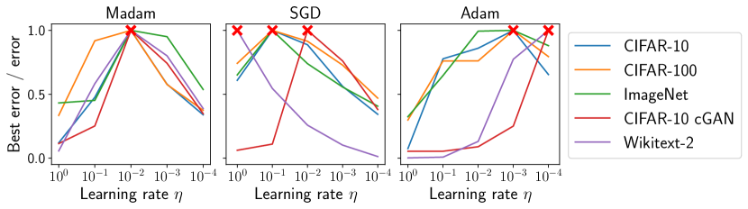
Figure 1: Learning rate tuning. We tuned the learning rate $\eta$ over a logarithmic grid on various deep learning benchmarks. For each run, a fixed $\eta$ is used without decay. For each optimiser and setting of $\eta$, we plot the best test error across all $\eta$ for that optimiser divided by the test error for that specific $\eta$, meaning that a value of $1.0$ (highlighted with a red cross) indicates the best setting of $\eta$ for that optimiser and task. For Madam, the best setting ($\eta=0.01$) was independent of task.

Table 1: Results after tuning the learning rate $\eta$. For each task, we compare to the better performing optimiser in $\{\text{SGD, Adam}\}$ and list the associated inital $\eta$. We quote top-1 test error, FID [36] and perplexity for the classifiers, GAN and transformer respectively. Lower is better in all cases. The mean and range are based on three repeats. Complete results are given in Table 3 in Appendix B.

Note: all Madam runs use initial learning rate $\mathit{\eta=0.01}$.
For all algorithms, $\mathit{\eta}$ is decayed by 10 when the loss plateaus.

Dataset	Task	Best Baseline	Baseline $\bm{\eta}$	Baseline Result	Madam $\bm{\eta}$	Madam Result
CIFAR-10	Resnet18	Adam	0.001	$6.6\pm 0.2$	0.01	$7.8\pm 0.2$
CIFAR-100	Resnet18	SGD	0.1	$29.1\pm 0.2$	0.01	$30.2\pm 0.1$
ImageNet	Resnet50	SGD	0.1	$24.1\pm 0.1$	0.01	$28.9\pm 0.1$
CIFAR-10	cGAN	Adam	0.0001	$23.9\pm 0.9$	0.01	$19\pm 2$
Wikitext-2	Transformer	SGD	1.0	$169.6\pm 0.6$	0.01	$173.3\pm 0.6$

In this section, we benchmark Madam (Algorithm 1) with weights represented in 32-bit floating point. In the next section, we shall benchmark $B$-bit Madam. The results in this section show that—across various tasks, including image classification, language modeling and image generation—Madam without learning rate tuning is competitive with a tuned SGD or Adam.

In Figure 1, we show the results of a learning rate grid search undertaken for Madam, SGD and Adam. The optimal learning rate setting for each benchmark is shown with a red cross. Notice that for Madam the optimal learning rate is in all cases $0.01$, whereas for SGD and Adam it varies.

In Table 1, we compare the final results using tuned learning rates for Adam and SGD and using $\eta=0.01$ for Madam. Madam’s results are competitive, and substantially better in the GAN experiment where SGD obtained FID $>30$. Madam performed worst on the Imagenet experiment, achieving a test error 4.8% worse than SGD. These results were attained using epoch budgets lifted from the baseline implementations.

Implementation details

The code for these experiments is to be found at https://github.com/jxbz/madam. Because bias terms are initialised to zero by default in Pytorch [37], a multiplicative update would have no effect on these parameters. Therefore we intialised the biases away from zero in some experiments, which led to slight performance improvements. Madam benefited from light tuning of the $\sigma^{*}$ hyperparameter (see Algorithm 1) which regularises the network by controlling the maximum size of the weights. In each experiment, $\sigma^{*}$ was set to be 1 to 5 times larger than the initialisation scale on a layerwise basis. Tuning $\sigma^{*}$ had a comparable effect on final performance to the effect of tuning weight decay in SGD. More experimental details are given in Appendix B.

6 Benchmarking $\bm{B}$-bit Madam

The results in this section demonstrate that $B$-bit Madam can be used to train networks that use 8–12 bits per weight, often with little to no loss in accuracy compared to an FP32 baseline. This compression level is in the range of 8–16 bits suggested by prior work [25, 28, 27]. However, we must emphasise the ease with which these results were attained. Just as Madam did not require learning rate tuning (see Figure 1), neither did $B$-bit Madam. In all 12-bit runs, a learning rate of $\eta=0.01$ combined with a base precision $\eta_{0}=0.001$ could be relied upon to achieve stable learning.

The results are given in Table 2. Though little deterioration is experienced at 12 bits, we believe that the results could be improved by making minor hyperparameter tweaks. For example, in the 12-bit ImageNet experiment we were able to reduce the error from $\sim 29\%$ to $\sim 25\%$ by borrowing layerwise parameter scales $\sigma^{*}$ (see Section 4.1) from a pre-trained model instead of using the standard Pytorch [37] initialisation scale. Still, it would be against the spirit of this work to present results with over-tuned hyperparameters.

To get more of a feel for the relative simplicity of our approach, we shall briefly comment on some of the subtleties introduced by prior work that $B$-bit Madam avoids. Studies often maintain higher-precision copies of the weights as part of their low-precision training process [29, 28]. For example, in their paper on 8-bit training, Wang et al. [28] actually maintain a 16-bit master copy of the weights. Furthermore, it is common to keep certain network layers such as the output layer at higher precision [27, 28, 29]. In contrast, we use the same bit width to represent every layer’s weights, and weights are both stored and updated in their $B$-bit representation.

Furthermore, we want to emphasise how natural it is to combine multiplicative updates with a logarithmic number system. Prior research on deep network training using logarithmic number systems has combined them with additive optimisation algorithms like SGD [30]. This necessitates tuning both the number system hyperparameters (dynamic range and base precision) and the optimisation hyperparameter (learning rate). As was demonstrated in Figure 1, tuning the SGD learning rate is already a computationally intensive task. Moreover, the cost of hyperparameter grid search grows exponentially in the number of hyperparameters.

Table 2: Benchmarking $B$-bit Madam. We tested 12-bit, 10-bit and 8-bit Madam on various tasks. The results for the FP32 baseline are reproduced from Table 1. For each result we give the mean and range over three repeats. In all experiments, an initial learning rate $\eta$ of $O(0.01)$ was used. In all 12-bit experiments, the base precision was chosen as $\eta_{0}=0.001$. In order to reduce the bit width from 12 to 8 bits, we increased the base precision $\eta_{0}$ of the numerical representation finding this to work better than the alternative: reducing the dynamic range of the numerical representation.

Dataset	Task	FP32 Madam	12-bit	10-bit	8-bit
CIFAR-10	Resnet18	$7.8\pm 0.2$	$7.0\pm 0.1$	$7.8\pm 0.3$	$8.6\pm 1.5$
CIFAR-100	Resnet18	$30.2\pm 0.1$	$27.6\pm 0.3$	$29.5\pm 0.3$	$33.9\pm 1.1$
ImageNet	Resnet50	$28.9\pm 0.1$	$31.1\pm 0.1$	$34.8\pm 0.3$	$50.5\pm 0.5$
CIFAR-10	cGAN	$19.3\pm 0.7$	$19.8\pm 0.8$	$23.4\pm 0.4$	$36\pm 6$
Wikitext-2	Transformer	$173.3\pm 0.6$	$182.3\pm 0.6$	$218.0\pm 0.6$	$262\pm 2$

Implementation details

The code for these experiments is to be found at https://github.com/jxbz/madam. The $B$-bit Madam hyperparameters are defined in Section 4.1. We choose the layerwise scale $\sigma^{*}$ in $B$-bit Madam following the same strategy as $\sigma^{*}$ in Madam: 1 to 5 times the default Pytorch [37] initialisation scale, except for biases where the default Pytorch initialisation is zero. We choose the initial learning rate $\eta$ to be $O(0.01)$ across all experiments. In the 12-bit experiments, we choose the base precision $\eta_{0}=0.001$. In the 10-bit and 8-bit experiments, a larger base precision is used—still satisfying $\eta_{0}\leq\eta=O(0.01)$. For each layer, we initialise the weights uniformly from:

$$\left\{\pm\sigma^{*}\mathrm{e}^{-k\eta_{0}}:k\in\{0,1,...,2^{B}-1\}\right\}.$$

Notice that $\eta_{0}$ sets the precision of the representation, and the dynamic range is given by $\exp{\left[(2^{B}-1)\eta_{0}\right]}$. For $B=12$ bits and base precision $\eta_{0}=0.001$ as used in the 12-bit experiments, the dynamic range is $60.0$ to 1 decimal place. Finally, during training the learning rate $\eta$ is decayed toward the base precision $\eta_{0}$ whenever the loss plateaus. See Appendix B for more detail.

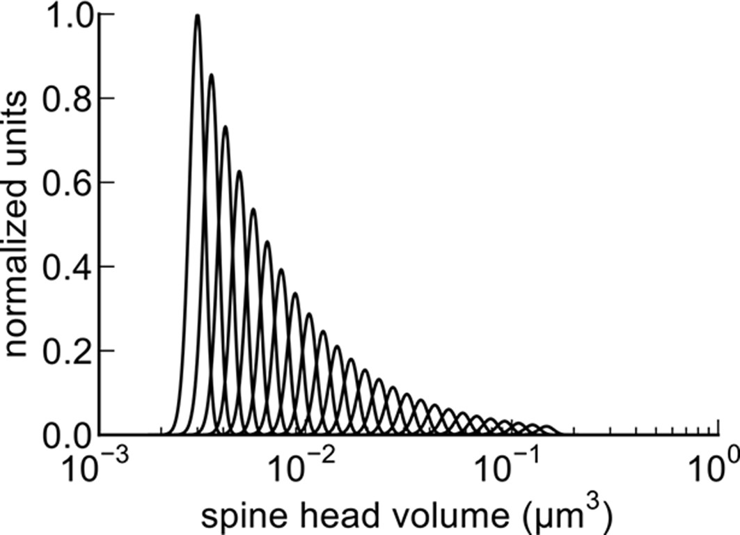
Figure 2: Upper left: the bfloat16 number system used in Google’s TPU chips [38]. Lower left: the logarithmic number system suggested by our theory. Right: the synaptic number system suggested by Bartol et al. [1] based on 3D electron microscope images of hippocampal neuropil in three adult male rats. Synapses are suggested to take 26 distinguishable strengths (believed to be correlated with spine head volume) on a logarithmic number system. This plot is reproduced from [1, Figure 8].

7 Discussion

After studying the optimisation properties of compositional functions, we have confirmed that neural networks may be trained via multiplicative updates to weights stored in a logarithmic number system. We shall now discuss possible implications for both chip design and neuroscience.

Computer number systems

In an effort to accelerate and reduce the cost of machine learning workflows, chip designers are currently exploring low precision arithmetic in both GPUs and TPUs. For example, Google has used bfloat16—or brain floating point—in their TPUs [38] and NVIDIA has developed a mixed precision GPU training system [39]. A basic question in the design of low-precision number systems is how the bits should be split between the exponent and mantissa. As shown in Figure 2 (left), bfloat16 opts for an 8-bit exponent and 7-bit mantissa. Our work supports a prior suggestion [30] that to represent network weights, a mantissa may not be needed at all.

Curiously, the same observation is made by Bartol et al. [1] in the context of neuroscience. In Figure 2 (right), we reproduce a plot from their paper that illustrates this. The authors suggest that the brain may use “a form of non-uniform quantization which efficiently encodes the dynamic range of synaptic strengths at constant precision”—or in other words, a logarithmic number system. The authors found that “spine head volumes ranged in size over a factor of 60 from smallest to largest”, where spine head volume is a correlate of synapse strength. Coincidentally, $B$-bit Madam with $B=12$ and base precision $\eta_{0}=0.001$ (as in our experiments) has the same dynamic range of $\exp[(2^{B}-1)\eta_{0}]\approx 60$.

Frozen signs and Dale’s principle

The neuroscientific principle that synapses cannot change sign is sometimes referred to as Dale’s principle [19]. When compositional functions are learnt via multiplicative updates, the signs of the weights are frozen and can be thought to satisfy Dale’s principle. This means that after training with multiplicative updates, there is no need to store the sign bits since they may be regenerated from the random seed. This could also impact hardware design since it would technically be possible to freeze a random sign pattern into the microcircuitry itself.

Plasticity in the brain

The precise mechanisms for plasticity in the brain are still under debate. Popular models include Hebbian learning and its variant spike time dependent plasticity, both of which adjust synapse strengths based on local firing history. Although these rules are usually modeled via additive updates, it has been suggested that multiplicative updates may better explain the available data—both in terms of the induced stationary distribution of synapse strengths, and also time-dependent observations [40, 41, 42]. For example, Loewenstein et al. [43] image dendritic spines in the mouse auditory cortex over several weeks. Upon finding that changes in spine size are “proportional to the size of the spine”, the authors suggest that multiplicative updates are at play.

In contrast to these studies that concentrate on matching candidate update rules to available data—and thus probing how the brain learns—this paper has focused on using perturbation theory and calculus to link update rules to the stability of network function. This is a complementary approach that may shed light on why the brain learns the way it does—paving the way, perhaps, for computer microarchitectures that mimic it.

8 Limitations and future work

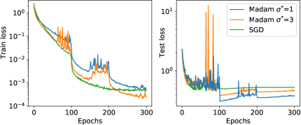
Figure 3: Convergence speed and effect of weight clipping. We plot the convergence curves of SGD and Madam on CIFAR-10. Two different weight clipping thresholds $\sigma^{*}$ are shown for Madam. Reducing the clipping threshold $\sigma^{*}$ can be seen to both stabilise and regularise the test performance.

There are two aspects of this work that we would like to understand better. The first is the role of the weight clipping threshold $\sigma^{*}$ (see Algorithm 1). Figure 3 shows a comparison between an SGD baseline and Madam with different weight clipping thresholds. As can be seen, a reduced clipping threshold seems to both stabilise and regularise the test loss. The stabilising role of weight clipping may be understood as follows: at the end of training, a learning algorithm can overfit the training set by simply scaling up the learnt weights (amplifying confidence on its current predictions). Since Madam can increase the weights exponentially (via compound growth over a number of iterations), this effect is particularly unstable and motivates explicit weight clipping. Still, needing to tune this clipping threshold is undesirable, and it would be better if there were a way to avoid it.

The second is the slight deterioration of Madam compared to Adam and SGD in Table 1. It is not immediately clear where this deterioration comes from. One possibility is that, since Madam freezes the sign pattern of weights from initialisation, the network is not expressive enough to represent the very best solutions. A workaround to this potential problem could involve finding a better way to initialise the sign pattern of the weights at the start of training. More generally, it is possible that we are missing some key idea that would close this performance gap.

Broader impact

This paper proposes that multiplicative update rules may be better suited to the compositional structure of neural networks than additive update rules. It concludes by discussing possible implications of this idea for chip design and neuroscience. The authors believe the work to be fairly neutral in terms of propensity to cause positive or negative societal outcomes.

References

Appendix A Proofs

See 1

Proof.

By the fundamental theorem of calculus,

$$\mathcal{L}(W+\Delta W)-\mathcal{L}(W)=\sum_{k=1}^{L}\left[g_{k}(W)^{T}\Delta W_{k}+\int_{0}^{1}\big{[}g_{k}(W+t\Delta W)-g_{k}(W)\big{]}^{T}\Delta W_{k}\,\mathrm{d}{t}\right].$$

The result follows by replacing the first term on the righthand side by the cosine formula for the dot product, and bounding the second term via the integral estimation lemma. ∎

See 1 See 1

Proof.

Using the gradient reliability estimate from deep relative trust, we obtain that:

$$\max_{t\in[0,1]}\frac{\|{g_{k}(W+t\Delta W)-g_{k}(W)}\|_{F}}{\|{g_{k}(W)}\|_{F}}\leq\max_{t\in[0,1]}\prod_{l=1}^{L}\left(1+\frac{\|{t\Delta W_{l}}\|_{F}}{\|{W_{l}}\|_{F}}\right)-1\leq\prod_{l=1}^{L}\left(1+\frac{\|{\Delta W_{l}}\|_{F}}{\|{W_{l}}\|_{F}}\right)-1.$$

Descent is guaranteed if the bracketed terms in Lemma 1 are positive. By the previous inequality, this will occur provided that:

$$\prod_{l=1}^{L}\left(1+\frac{\|{\Delta W_{l}}\|_{F}}{\|{W_{l}}\|_{F}}\right)<1+\cos\theta_{k}\qquad(\text{for all }k=1,...,L)$$ (6)

where $\theta_{k}$ measures the angle between $\Delta W_{k}$ and $-g_{k}(W)$. For the update in Equation 3,

$$W+\Delta W=W\odot(1-\eta\operatorname*{sign}W\odot\operatorname*{sign}g(W)).$$

Therefore the perturbation is given by $\Delta W=-\eta\,|{W}|\odot\operatorname*{sign}g(W)$. For this perturbation, $\|{\Delta W_{*}}\|_{F}/\|{W_{*}}\|_{F}=\eta$ for any possible subset of weights $W_{*}$. Also, letting $\measuredangle(\cdot,\cdot)$ return the angle between its arguments, $\theta_{k}$ and $\gamma_{k}$ are related by:

$$\theta_{k} :=\measuredangle(\Delta W_{k},-g_{k}(W))$$

$$=\measuredangle(-\eta\,|{W_{k}}|\odot\operatorname*{sign}g_{k}(W),-g_{k}(W))$$

$$=\measuredangle(|{W_{k}}|\odot\operatorname*{sign}g_{k}(W),g_{k}(W))$$

$$=\measuredangle(|{W_{k}}|,|{g_{k}(W)}|)$$

$$=:\gamma_{k}.$$

Substituting these two results back into Equation 6 and rearranging, we are done. ∎

Table 3: Complete results for FP32 Madam. We quote top-1 error, FID [36] and perplexity for the classifiers, GAN and transformer respectively. Lower is better in all cases. The mean result is quoted with a range based on three repeats.

Note: all Madam runs use initial learning rate $\mathit{\eta=0.01}$.
For all algorithms, $\mathit{\eta}$ is decayed by 10 when the loss plateaus.

Dataset	Adam $\bm{\eta}$	Adam train	Adam test	SGD $\bm{\eta}$	SGD train	SGD test	Madam $\bm{\eta}$	Madam train	Madam test
CIFAR-10	0.001	$0.01\pm 0.01$	$6.6\pm 0.2$	0.1	$0.01\pm 0.01$	$8.2\pm 1.3$	0.01	$0.01\pm 0.01$	$7.8\pm 0.2$
CIFAR-100	0.001	$0.02\pm 0.01$	$29.8\pm 0.4$	0.1	$0.03\pm 0.01$	$29.1\pm 0.2$	0.01	$2.35\pm 0.08$	$30.2\pm 0.1$
ImageNet	0.01	$19.8\pm 0.2$	$26.7\pm 0.3$	0.1	$17.7\pm 0.1$	$24.1\pm 0.1$	0.01	$25.4\pm 0.1$	$28.9\pm 0.1$
cGAN	0.0001	$23.1\pm 0.8$	$23.9\pm 0.9$	0.01	$34\pm 1$	$34\pm 1$	0.01	$19\pm 2$	$19\pm 2$
Wikitext-2	0.0001	$109.8\pm 0.5$	$173.4\pm 0.9$	1.0	$149.9\pm 0.2$	$169.6\pm 0.6$	0.01	$126.9\pm 0.2$	$173.3\pm 0.6$

Appendix B Experimental details

FP32 Madam

The initial learning rate was set to $\eta=0.01$ across all tasks, while the weight clipping threshold $\sigma^{*}$ was tuned over the range 1 to 5. The learning rate schedule was set specific to each task, although the general strategy was to decay the learning rate upon plateau of the loss.

$\bm{B}$-bit Madam

For 12-bit Madam, the base precision $\eta_{0}$ was set to 0.001 across all tasks. To reduce precision to 10 bits and 8 bits, we maintained the same dynamic range as for 12 bits by increasing the base precision $\eta_{0}$. For example, in all the image classification experiments, the initial learning rate $\eta$ was set to 0.016 for all bit widths, while the learning rate was decayed to 0.001 in the 12-bit experiments, 0.004 in the 10-bit experiments and never decayed in the 8-bit experiments. In the GAN and transformer experiments, the initial learning rate $\eta$ was set to 0.01. The difference between an initial learning rate of $0.016$ and $0.01$ was not highly significant—the learning rate of 0.016 was chosen to be compatible with code that decayed the learning rate by powers of two. The weight clipping threshold $\sigma^{*}$ was set to the value used in FP32 Madam for each task.

CIFAR-10 classification

We evaluated the different optimisers on the CIFAR-10 dataset [44] using a Resnet-18 model [45]. CIFAR-10 consists of 60,000 images in 10 different classes. For simplicity, we switched off the learnable affine parameters in batch norm. The network was trained for 300 epochs, and we used a fixed learning rate decay schedule that decayed every 100 epochs.

CIFAR-100 classification

The CIFAR-100 dataset is similar to CIFAR-10, but contains 100 classes containing 600 images each [44]. Again, we used a Resnet-18 model with the batch norm affine parameters switched off. The other hyperparameters were chosen in the same way as for CIFAR-10, including the epoch budget and learning rate decay strategy.

ImageNet classification

The ILSVRC2012 ImageNet dataset consists of 1.2 million images belonging to 1,000 classes [46]. We used a Resnet-50 network architecture to benchmark the optimisers [45]. Again, we switched off the affine parameters in batch norm for simplicity. The network was trained for 90 epochs. We applied a learning rate warm-up for the first 5 epochs of training, and decayed the learning rate after every 30 epochs.

CIFAR-10 GAN

We trained a class-conditional generative adversarial network (cGAN) using a custom implementation of the BigGAN architecture [47], to learn to generate the CIFAR-10 dataset [44]. The same learning rate was used in both the generator and discriminator. The networks were trained for 120 epochs. The learning rate was decayed after 100 epochs of training, by a factor of 10 in the FP32 experiments and to the base precision in the $B$-bit experiments. Bias parameters were initialised from a Normal distribution with mean zero and variance 0.01.

Wikitext-2 transformer

WikiText-2 is a language modeling dataset that contains over 100 million tokens extracted from Wikipedia [48]. We trained a transformer network architecture [49] that was smaller than the transformers that are typically used for this task, explaining the general degradation of results compared to the state of the art for this dataset. The network was trained for 20 epochs with a single learning rate decay at epoch 10. In 12-bit Madam, decaying the learning rate to 0.005 rather than to the base precision of 0.001 slightly improved the results.

References

- Bartol et al. [2015] Thomas M. Bartol, Jr., Cailey Bromer, Justin Kinney, Michael A. Chirillo, Jennifer N. Bourne, Kristen M. Harris, and Terrence J. Sejnowski. Nanoconnectomic upper bound on the variability of synaptic plasticity. eLife, 2015.
- Baker and Hammerstrom [1989] Tom Baker and Dan Hammerstrom. Characterization of artificial neural network algorithms. In International Symposium on Circuits and Systems, 1989.
- Horowitz [2014] Mark Horowitz. Computing’s energy problem (and what we can do about it). In International Solid-State Circuits Conference, 2014.
- Sze et al. [2017] Vivienne Sze, Yu-Hsin Chen, Tien-Ju Yang, and Joel Emer. Efficient processing of deep neural networks: A tutorial and survey. Proceedings of the IEEE, 2017.
- Bernstein et al. [2020] Jeremy Bernstein, Arash Vahdat, Yisong Yue, and Ming-Yu Liu. On the distance between two neural networks and the stability of learning. In Neural Information Processing Systems, 2020.
- Littlestone [1988] Nick Littlestone. Learning quickly when irrelevant attributes abound: A new linear-threshold algorithm. Machine Learning, 1988.
- Kivinen and Warmuth [1997] Jyrki Kivinen and Manfred K. Warmuth. Exponentiated gradient versus gradient descent for linear predictors. Information and Computation, 1997.
- Freund and Schapire [1997] Yoav Freund and Robert E Schapire. A decision-theoretic generalization of on-line learning and an application to boosting. Journal of Computer and System Sciences, 1997.
- Grigoriadis and Khachiyan [1995] Michael D. Grigoriadis and Leonid G. Khachiyan. A sublinear-time randomized approximation algorithm for matrix games. Operations Research Letters, 1995.
- Arora et al. [2012] Sanjeev Arora, Elad Hazan, and Satyen Kale. The multiplicative weights update method: a meta-algorithm and applications. Theory of Computing, 2012.
- Dhillon and Tropp [2008] Inderjit S. Dhillon and Joel A. Tropp. Matrix nearness problems with Bregman divergences. SIAM Journal on Matrix Analysis and Applications, 2008.
- Bottou et al. [2018] Léon Bottou, Frank E. Curtis, and Jorge Nocedal. Optimization methods for large-scale machine learning. SIAM Review, 2018.
- Zhang et al. [2020] Jingzhao Zhang, Tianxing He, Suvrit Sra, and Ali Jadbabaie. Why gradient clipping accelerates training: A theoretical justification for adaptivity. In International Conference on Learning Representations, 2020.
- Azizan et al. [2019] Navid Azizan, Sahin Lale, and Babak Hassibi. Stochastic mirror descent on overparameterized nonlinear models: Convergence, implicit regularization, and generalization, 2019. arXiv:1906.03830.
- Neyshabur et al. [2015] Behnam Neyshabur, Ruslan Salakhutdinov, and Nathan Srebro. Path-SGD: Path-normalized optimization in deep neural networks. In Neural Information Processing Systems, 2015.
- You et al. [2017] Yang You, Igor Gitman, and Boris Ginsburg. Scaling SGD batch size to 32K for Imagenet training. Technical Report UCB/EECS-2017-156, University of California, Berkeley, 2017.
- You et al. [2020] Yang You, Jing Li, Sashank Reddi, Jonathan Hseu, Sanjiv Kumar, Srinadh Bhojanapalli, Xiaodan Song, James Demmel, Kurt Keutzer, and Cho-Jui Hsieh. Large batch optimization for deep learning: Training BERT in 76 minutes. In International Conference on Learning Representations, 2020.
- van Vreeswijk and Sompolinsky [1996] Carl van Vreeswijk and Haim Sompolinsky. Chaos in neuronal networks with balanced excitatory and inhibitory activity. Science, 1996.
- Amit et al. [1989] Daniel J. Amit, K. Y. Michael Wong, and Colin Campbell. Perceptron learning with sign-constrained weights. Journal of Physics A, 1989.
- Akira Iwata et al. [1989] Akira Iwata, Yukio Yoshida, Satoshi Matsuda, Yukimasa Sato, and Nobuo Suzumura. An artificial neural network accelerator using general purpose 24 bit floating point digital signal processors. In International Joint Conference on Neural Networks, 1989.
- Holt and Hwang [1993] Jordan L. Holt and Jenq-Neng Hwang. Finite precision error analysis of neural network hardware implementations. Transactions on Computers, 1993.
- Courbariaux et al. [2015] Matthieu Courbariaux, Yoshua Bengio, and Jean-Pierre David. BinaryConnect: Training deep neural networks with binary weights during propagations. In Neural Information Processing Systems, 2015.
- Hubara et al. [2018] Itay Hubara, Matthieu Courbariaux, Daniel Soudry, Ran El-Yaniv, and Yoshua Bengio. Quantized neural networks: Training neural networks with low precision weights and activations. Journal of Machine Learning Research, 2018.
- Zhou et al. [2017] Aojun Zhou, Anbang Yao, Yiwen Guo, Lin Xu, and Yurong Chen. Incremental network quantization: Towards lossless CNNs with low-precision weights, 2017. arXiv:1702.03044.
- Gupta et al. [2015] Suyog Gupta, Ankur Agrawal, Kailash Gopalakrishnan, and Pritish Narayanan. Deep learning with limited numerical precision. In International Conference on Machine Learning, 2015.
- Müller and Indiveri [2015] Lorenz K. Müller and Giacomo Indiveri. Rounding methods for neural networks with low resolution synaptic weights, 2015. arXiv:1504.05767.
- Sun et al. [2019] Xiao Sun, Jungwook Choi, Chia-Yu Chen, Naigang Wang, Swagath Venkataramani, Vijayalakshmi Srinivasan, Xiaodong Cui, Wei Zhang, and Kailash Gopalakrishnan. Hybrid 8-bit floating point (HFP8) training and inference for deep neural networks. In Neural Information Processing Systems, 2019.
- Wang et al. [2018] Naigang Wang, Jungwook Choi, Daniel Brand, Chia-Yu Chen, and Kailash Gopalakrishnan. Training deep neural networks with 8-bit floating point numbers. In Neural Information Processing Systems, 2018.
- Wu et al. [2018] Shuang Wu, Guoqi Li, Feng Chen, and Luping Shi. Training and inference with integers in deep neural networks. In International Conference on Learning Representations, 2018.
- Lee et al. [2017] Edward H. Lee, Daisuke Miyashita, Elaina Chai, Boris Murmann, and S. Simon Wong. LogNet: Energy-efficient neural networks using logarithmic computation. In International Conference on Acoustics, Speech and Signal Processing, 2017.
- Vogel et al. [2018] Sebastian Vogel, Mengyu Liang, Andre Guntoro, Walter Stechele, and Gerd Ascheid. Efficient hardware acceleration of CNNs using logarithmic data representation with arbitrary log-base. In International Conference on Computer-Aided Design, 2018.
- Rumelhart et al. [1986] David E. Rumelhart, Geoffrey E. Hinton, and Ronald J. Williams. Learning representations by back-propagating errors. Nature, 1986.
- Huang et al. [2017] Gao Huang, Zhuang Liu, Laurens van der Maaten, and Kilian Q. Weinberger. Densely connected convolutional networks. In Computer Vision and Pattern Recognition, 2017.
- Kingma and Ba [2015] Diederik P. Kingma and Jimmy Ba. Adam: A Method for Stochastic Optimization. In International Conference on Learning Representations, 2015.
- Tieleman and Hinton [2012] Tijmen Tieleman and Geoffrey E. Hinton. Lecture 6.5—RMSprop: Divide the gradient by a running average of its recent magnitude. COURSERA: Neural Networks for Machine Learning, 2012.
- Heusel et al. [2017] Martin Heusel, Hubert Ramsauer, Thomas Unterthiner, Bernhard Nessler, and Sepp Hochreiter. GANs trained by a two time-scale update rule converge to a local Nash equilibrium. In Neural Information Processing Systems, 2017.
- Paszke et al. [2019] Adam Paszke, Sam Gross, Francisco Massa, Adam Lerer, James Bradbury, Gregory Chanan, Trevor Killeen, Zeming Lin, Natalia Gimelshein, Luca Antiga, Alban Desmaison, Andreas Kopf, Edward Yang, Zachary DeVito, Martin Raison, Alykhan Tejani, Sasank Chilamkurthy, Benoit Steiner, Lu Fang, Junjie Bai, and Soumith Chintala. Pytorch: An imperative style, high-performance deep learning library. In Neural Information Processing Systems, 2019.
- Kalamkar et al. [2019] Dhiraj D. Kalamkar, Dheevatsa Mudigere, Naveen Mellempudi, Dipankar Das, Kunal Banerjee, Sasikanth Avancha, Dharma Teja Vooturi, Nataraj Jammalamadaka, Jianyu Huang, Hector Yuen, Jiyan Yang, Jongsoo Park, Alexander Heinecke, Evangelos Georganas, Sudarshan Srinivasan, Abhisek Kundu, Misha Smelyanskiy, Bharat Kaul, and Pradeep Dubey. A study of bfloat16 for deep learning training, 2019. arXiv:1905.12322.
- Micikevicius et al. [2018] Paulius Micikevicius, Sharan Narang, Jonah Alben, Gregory Diamos, Erich Elsen, David Garcia, Boris Ginsburg, Michael Houston, Oleksii Kuchaiev, Ganesh Venkatesh, and Hao Wu. Mixed precision training. In International Conference on Learning Representations, 2018.
- van Rossum et al. [2000] Mark C. van Rossum, Guo-qiang Bi, and Gina G. Turrigiano. Stable Hebbian learning from spike timing-dependent plasticity. Journal of Neuroscience, 2000.
- Barbour et al. [2007] Boris Barbour, Nicolas Brunel, Vincent Hakim, and Jean-Pierre Nadal. What can we learn from synaptic weight distributions? Trends in Neurosciences, 2007.
- Buzsáki and Mizuseki [2014] György Buzsáki and Kenji Mizuseki. The log-dynamic brain: how skewed distributions affect network operations. Nature Reviews Neuroscience, 2014.
- Loewenstein et al. [2011] Yonatan Loewenstein, Annerose Kuras, and Simon Rumpel. Multiplicative dynamics underlie the emergence of the log-normal distribution of spine sizes in the neocortex in vivo. Journal of Neuroscience, 2011.
- Krizhevsky [2009] Alex Krizhevsky. Learning multiple layers of features from tiny images. Technical report, University of Toronto, 2009.
- He et al. [2016] Kaiming He, Xiangyu Zhang, Shaoqing Ren, and Jian Sun. Deep residual learning for image recognition. In Computer Vision and Pattern Recognition, 2016.
- Deng et al. [2009] Jia Deng, Wei Dong, Richard Socher, Li-Jia Li, Kai Li, and Li Fei-Fei. Imagenet: A large-scale hierarchical image database. In Computer Vision and Pattern Recognition, 2009.
- Brock et al. [2019] Andrew Brock, Jeff Donahue, and Karen Simonyan. Large scale GAN training for high fidelity natural image synthesis. In International Conference on Learning Representations, 2019.
- Merity et al. [2017] Stephen Merity, Caiming Xiong, James Bradbury, and Richard Socher. Pointer sentinel mixture models. In International Conference on Learning Representations, 2017.
- Vaswani et al. [2017] Ashish Vaswani, Noam Shazeer, Niki Parmar, Jakob Uszkoreit, Llion Jones, Aidan N Gomez, Łukasz Kaiser, and Illia Polosukhin. Attention is all you need. In Neural Information Processing Systems, 2017.