Hierarchical stock assessment methods improve management performance in multi-species, data-limited fisheries.

Abstract

Managers of multi-species fisheries aim to balance harvest of multiple interacting species that vary in abundance and productivity. Technical interactions are a defining characteristic of multi-species fisheries, and are often ignored when setting catch limits or target exploitation rates, despite their effect on the ability to balance multi-species harvest. Balancing harvest is more difficult when stock assessments are impossible to perform due to data-limitations, involving inter alia short time series of fishery independent observations, poor catch monitoring, limited biological data, and spatial mismatching of harvest decisions to system structure. In this paper, we asked whether using hierarchical, data-limited stock assessment methods to set catch limits improved management performance in data-limited, multi-species fisheries. Management performance of five alternative stock assessment methods was evaluated by using them to set harvest levels targeting multi-species maximum yield in a multi-species flatfish fishery, including single-species and hierarchical multi-species models, and methods that pooled data across species and spatial strata, with catch outcomes of each method under three data scenarios compared to catch under an omniscient manager simulation. Operating models included technical interactions between species intended to produce choke effects often observed in output controlled multi-species fisheries. Hierarchical multi-species models outperformed all other methods under data-poor and data-moderate scenarios, and outperformed single-species models under the data-rich scenario. Hierarchical models were least sensitive to prior precision, sometimes improving in performance when prior precision was reduced. Choke effects were found to both positive and negative effects, sometimes leading to underfishing of non-choke species, but at other times preventing overfishing of non-choke species. We highlight the importance of including technical interactions in multi-species assessment models and management objectives, how choke species can indicate mismatches between management objectives and system dynamics, and recommend hierarchical multi-species models for multi-species fishery management systems.

abstract

1 Introduction

Managers of multi-species fisheries aim to balance harvest of multiple interacting target and non-target species that vary in abundance and productivity. Among-species variation in productivity implies variation in single-species optimal harvest rates, and, therefore, differential responses to exploitation. Single-species optimal harvest rates (e.g., the harvest rate associated with maximum sustainable yield) typically ignore both multi-species trophic interactions that influence individual demographic rates (Gislason, 1999; Collie and Gislason, 2001), and technical interactions that make it virtually impossible to simultaneously achieve the optimal harvest rate for all species (Pikitch, 1987).

Technical interactions among species that co-occur in non-selective fishing gear are a defining characteristic of multi-species fisheries (Pikitch, 1987; Punt et al., 2002) and, therefore, play a central role in multi-species fisheries management outcomes for individual species (Ono et al., 2017; Kempf et al., 2016). Catch limits set for individual species without considering technical interactions subsequently lead to sub-optimal fishery outcomes (Ono et al., 2017; Punt et al., 2011a, 2020). For example, under-utilization of catch limits could occur when technically interacting quota species are caught at different rates (i.e., catchability) by a common gear, leading to a choke constraint in which one species quota is filled before the others (Baudron and Fernandes, 2015). Choke constraints are generally considered negative outcomes for multi-species fishery performance, because they reduce harvester profitability as increasingly rare quota for choke species may limit access to fishing grounds, as well as driving quota costs above the landed value of the choke species (Mortensen et al., 2018).

Setting catch limits for individual species in any fishery usually requires an estimate of species abundance, which continues to be a central challenge of fisheries stock assessment (Hilborn and Walters, 1992; Quinn, 2003; Maunder and Piner, 2015), especially when species data are insufficient for stock assessment models. Where such data limitations exist, data pooling is sometimes used to extend stock assessments to complexes of similar, interacting stocks of fish (Appeldoorn, 1996). A couple of examples include pooling data for a single species across multiple spatial strata when finer scale data are unavailable or when fish are believed to move between areas at a sufficiently high rate (Benson et al., 2015; Punt et al., 2018), and pooling data for multiple species of the same taxonomic group within an area when data are insufficient for individual species or during development of new fisheries (DeMartini, 2019). Data-pooled estimates of productivity represent means across the species complex; therefore the general cost of such pooling approaches is that catch limits will tend to overfish unproductive species and underfish productive ones (Gaichas et al., 2012). Hierarchical stock assessment models may help reduce these problems by representing a compromise between uninformative single-species single-species approaches and problematic data-pooling approaches. In particular, hierarchical models allow data sharing between multiple species within a complex via hierarchical shrinkage prior distributions on model parameters that represent biological similarities or technical interactions (Thorson et al., 2015). Shared priors shrink species-specific parameters towards an estimated complex level mean value, improving model convergence for data-poor species and basing estimates more on available data than strong a priori assumptions like fixed (i.e. known) parameters, identical parameters among species, or strongly informative priors (Jiao et al., 2009, 2011; Punt et al., 2011b).

Although hierarchical stock assessments produce better estimates of species biomass and productivity than single-species methods in data-limited contexts, it remains unclear whether such improved statistical performance translates into better management outcomes (Johnson and Cox, 2018). On one hand, improving assessment model statistical performance may sacrifice future fishery benefits of adaptive learning (Walters, 1986), as large assessment errors caused by poor quality data in the present may generate high contrast data that are more informative in the future. Alternatively, adaptive learning may fail to occur in a reasonable time in the presence of large errors, leading to stock collapse or harvesters divesting from the fishery because of over- or under-exploitation. Improving the rate of adaptive learning may be possible via hierarchical modeling of spatially replicated groundfish stocks, because the shared priors take lessons learned from responses to disturbances in one area and use them to improve stock assessments in other areas (Collie and Walters, 1991).

In this paper, we investigated whether hierarchical stock assessment models improved management performance in a simulated multi-species, data-limited fishery. The simulated fishery was modeled on a complex of Dover sole, English sole, and southern rock sole - three species of right-eyed flounders (Pleuronectidae spp.) - Dover sole (Microstomus pacificus), English sole (Parophrys vetulus), and southern rock sol (Lepidopsetta bilineata) - fished off the coast of British Columbia, Canada, in three spatial management areas. Closed-loop feedback simulation was used to estimate fishery outcomes when catch limits were set based on estimates of biomass from single-species, data-pooling, and hierarchical state-space surplus production models under three data scenarios. Assessment models were either fit to species specific data as single-species or hierarchical multi-species models, or fit to data pooled spatially across management units, pooled across species within a spatial management unit, or totally aggregated across both species and spatial management units. Management performance of each assessment approach was measured as cumulative absolute loss in catch, measured against optimal catch trajectories generated by an omniscient manager, who could set annual effort to maximize total multi-species/multi-stock complex yield given perfect knowledge of all future recruitments (Walters, 1998; Martell et al., 2008).

2 Methods

2.1 British Columbia’s flatfish fishery

British Columbia’s multi-species complex of right-eyed flounders is a technically interacting group of flatfishes managed across the whole BC coast. Although there are several right-eyed flounders in BC waters, we focus on Dover sole, English sole, and Rock sole. Taken together, these species comprise a multi-stock complex (DER complex), managed as part of the BC multi-species groundfish fishery.

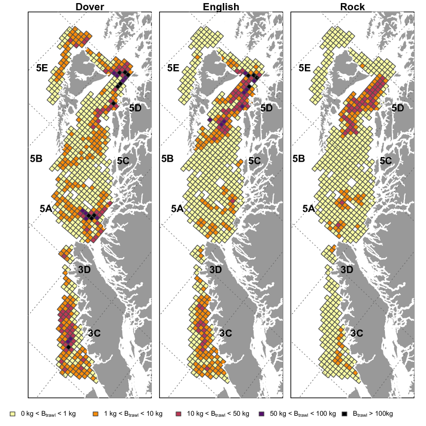
Figure 1: Mininum trawlable survey biomass $B_{trawl}$ estimates for DER complex species on the BC coast, aggregated to a 10km square grid. Estimates are produced by scaling average trawl survey ($kg/m^{2}$) density values in each grid cell by the cell’s area in $m^{2}$. Locations that do not show a coloured grid cell do not have any survey blocks from which to calculate relative biomass. Survey density for each grid cell is calculated from data for the Hecate Strait Assemblage Survey and the BC Groundfish Trawl Synoptic Survey, stored in the GFBio data base maintained at the Pacific Biological Station of Fisheries and Oceans, Canada. Thick black lines delineate the major statistical areas 3CD and 5ABCDE used for groundfish management BC, while the dashed grey lines makr out latitude and longitude, indicating the rotation of the coordinates to save space. The full colour figure is available in the online version of the article.

The DER complex is managed in three spatially distinct stock areas (Figure 1) (Fisheries and Oceans, Canada, 2015). From north to south, the first stock area - Hecate Strait/Haida Gwaii (HSHG) - corresponds to BC groundfish management area 5CDE, extending from Dixon Entrance and north of Haida Gwaii, south through Hecate Strait. The second stock area - Queen Charlotte Sound (QCS) - corresponds to BC groundfish management area 5AB, extending from the southern tip of Haida Gwaii to the northern tip of Vancouver Island. Finally, the third area - West Coast of Vancouver Island (WCVI) - corresponds to groundfish management area 3CD, extending from the northern tip of Vancouver Island south to Juan de Fuca Strait.

Each area had two commercial catch rate series and at least one survey biomass index time series for each species (Table 1). The two commercial fishery catch-per-unit-effort series span 1976 - 2016, split between a historical trawl fishery (1976 - 1995) and a modern trawl fishery (1996 - 2016), with the split corresponding to pre- and post-implementation of an at-sea-observer program, respectively. The fishery independent trawl survey biomass indices were the biennial Hecate Strait Assemblage survey in the HSHG area (1984 - 2002), and the Groundfish Multi-species Synoptic Survey, with separate biennial legs in all three stock areas (2003 - 2016).

2.2 Closed-loop feedback simulation framework

Closed-loop simulation is often used to evaluate proposed feedback management systems. In fisheries, closed-loop simulation evaluates fishery management system components, such as stock assessment models or harvest decision rules, by simulating repeated applications of these components, along with propagating realistic errors in monitoring data, stock assessment model outputs, and harvest advice (de la Mare, 1998; Cox and Kronlund, 2008; Cox et al., 2013). At the end of the simulation, pred-defined performance metrics are used to determine the relative performance of the system components being tested.

Our closed-loop simulation framework included a stochastic operating, representing the stock and fishery dynamics, as well as an observation model, and an assessment model component that estimated stock biomass from simulated observations and fishery catches. The operating model simulated population dynamics of a spatially stratified, multi-species flatfish complex in response to a multi-species trawl fishery in each of the three stock areas. Although total fishing effort was not restricted across the entire area, effort in each individual area was allocated such that no species-/area-specific catch exceeded the species-/area-specific total allowable catch (TAC). Within an area, fishing effort was allowed to increase until at least one species-/area-specific TAC was fully caught.

The simulation projected population dynamics for all nine stocks forward in time for $32$ years, with annual simulated assessments, harvest decisions, and catch removed from the population from 2017 - 2048. The following four steps summarise the closed-loop simulation procedure for each projection year $t$:

1. Update stochastic population dynamics and generate new realized catch $C_{s,p,t}(E_{p,t})$ in each area from effort (eq 1);

2. Generate new observation data $I_{s,p,f,t}$ (eqs 4-11)

3. Apply an assessment model (defined below) to estimate the spawning biomass for the upcoming year $\hat{B}_{s,p,t+1}$ (eq 3);

4. Apply a harvest rate to generate a total allowable catch $TAC_{s,p,t+1}$ (eqs 12 - 16);

5. Allocate effort $E_{p,t+1}$ to fully realise at least one TAC in each stock area (eq 2).

2.2.1 Operating Model

The operating model (OM) was a multi-species, multi-stock age- and sex-structured population dynamics model (Appendix A). Population life-history parameters for the operating model were estimated by fitting a hierarchical age- and sex-structured model to data from the real DER complex (Johnson, Cox and Knowler, in Prep).

Fishing mortality for individual stocks was scaled to commercial trawl effort via species-specific catchability parameters, i.e.,

$$F_{s,p,t}=q^{F}_{s,p}\cdot E_{p,t},$$ (1)

where $F_{s,p,t}$ is the fishing mortality rate applied to species $s$ in stock-area $p$ by fleet $f$ in year $t$, and $q^{F}_{s,p}$ is the commercial catchability coefficient scaling trawl effort $E_{p,t}$ in area $p$ to fishing mortality (Table 2) [Johnson and Cox, in prep].

The above effort model implies a multi-species maximum yield for the trawl fishery in each area, depending on individual species productivity, commercial trawl catchability, and relative catchabilities among species in the area (Pikitch, 1987; Punt et al., 2011a), i.e.,

$$MSY_{MS,p}=\max_{E}Y_{MS}\left(E,q^{F}_{1,p},q^{F}_{2,p},q^{F}_{3,p},Q_{p}\right),$$

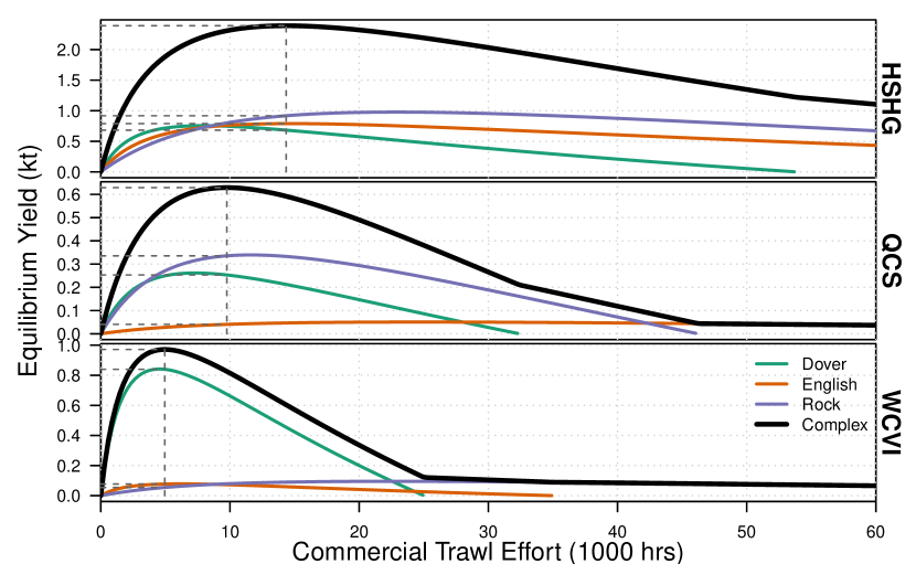
Figure 2: Operating model equilibrium yield curves for a given fishing effort for the nine DER complex management units, as well as complex yield curves within each stock area. Each panel shows the three individual DER complex species yield curves within a given stock area in different colours, and the complex yield curve found by summing the three yield curves as a thick black line.

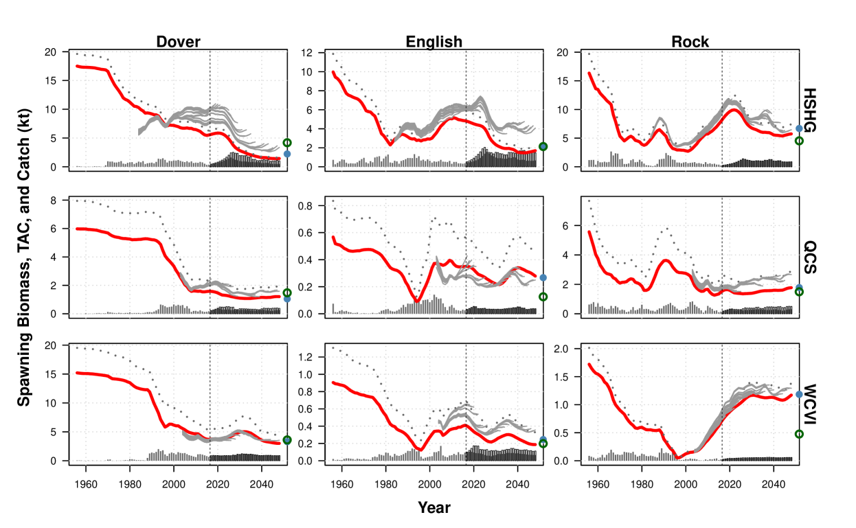
Figure 2: Operating model spawning stock biomass (red line), commercial trawl vulnerable biomass (grey dotted line), retrospective assesment model estimates of spawning stock biomass (thin grey/purple lines), and catch and TACs (grey bars) from the first simulation replicate in the Poor data quality scenario under the hierarchical multi-stock assessment model when hierarchical shrinkage prior SDs were $\sigma_{U_{MSY}}=\tau_{q}=0.5$. Catch bars show realised catch in grey for the whole simulation period, and unfilled bars in the projection period show the difference between MP set TACs and realised catch. Coloured circles on the right hand vertical axis show the biomass level associated with the multi-species (closed blue circle) and single-species (open green circle) maximum sustainable yield.

where $E$ is the total commercial trawl fishing effort, $q_{s,p}$ is the commerical trawl catchability coefficient scaling fishing effort to fishing mortality for species $s$ in area $p$, and $Q_{p}$ is the set of life-history parameters for all DER complex species in area $p$. The function $Y_{MS}$ is the total multi-species yield in area $p$ as a function of fishing effort $E_{p}$ (Figure 2, heavy black lines), defined as the sum of species-specific equilibrium yields

$$Y_{MS,p}\left(E_{p},q^{F}_{1,p},q^{F}_{2,p},q^{F}_{3,p},Q_{p}\right)=\sum^{3}_{s=1}Y_{SS,s,p}(E_{p},q_{s,p},Q_{s,p}),$$

where $Q_{s,p}$ is the subset of $Q_{p}$ containing life history parameters for species $s$ in area $p$, and the function $Y_{SS,s,p}$ is the traditional single-species yield curve expressed as a function of effort rather than fishing mortality (Figure 2, coloured lines).

The level of fishing effort producing multi-species maximum yield $MSY_{MS,p}$ in area $p$ is defined as

$$E_{MSY,p}={\mathop{\mathrm{arg\,max}}}_{E}Y_{MS}\left(E,q^{F}_{1,p},q^{F}_{2,p},q^{F}_{3,p},Q_{p}\right),$$

with arguments defined above (Figure 2, vertical dashed line). The fishing effort level $E_{MSY,p}$ has an associated equilibrium biomass $B_{MSY,MS,s,p}$ and yield

$$MSY_{MS,s,p}=Y_{SS,s,p}(E_{MSY,p},q^{F}_{s,p},Q_{s,p})$$

for each species $s$ (Figure 2, three lower horizontal dashed lines showing individual species yield), which differ from the single-species $B_{MSY}$ and $MSY$ when commercial catchability scalars differ between species.

For simulated fishing in the projection time period, we allocated maximum fishing effort to each area, defined as the effort required to fully utilize the TAC of at least one species, while never exceeding the TAC of any one of the three species, i.e.,

$$E_{p,t+1}=\max\{E~{}|~{}C_{s,p,t+1}(E)\leq TAC_{s,p,t+1}\forall s\},$$ (2)

where $C_{s,p,t+1}(E)$ is the catch of species $s$ when effort $E$ is applied in area $p$ in year $t+1$ (the method for determining TACs is explained below). We used maximum effort instead of an explicit effort dynamics model because the former was adequate for understanding the relative management performance of the assessment models that we tested. Furthermore, the maximum effort model may be simplified over reality, but it did an adequate job of capturing choke effects observed in the real BC groundfish fishery system.

2.2.2 Surplus production stock assessment models

At each time step $t$, simulated annual assessments were used to estimate the expected future spawning biomass estimate $\hat{B}_{t+1}$ via a state-space Schaefer production model (Schaefer, 1957; Punt et al., 2002), modified to better approximate the biomass-yield relationship underlying the age-/sex-structured operating model (Pella and Tomlinson, 1969; Winker et al., 2018). We extended the Johnson and Cox (2018) hierarchical state-space model to fit a multi-species, spatially stratified complex, as well as fit a single-stock model to data from individual or data-pooled stocks, via the biomass equation

$$B_{s,p,t+1}=\left[B_{s,p,t}+U_{MSY,s,p}\cdot\frac{m_{s,p}}{m_{s,p}-1}\cdot B_{s,p,t}\cdot\left(1-\frac{1}{m_{s,p}}\cdot\left(\frac{B_{s,p,t}}{B_{MSY,s,p}}\right)^{m_{s,p}-1}\right)-C_{s,p,t}\right]e^{\zeta_{s,p,t}},$$ (3)

where $B_{MSY}$ (optimal biomass) and $U_{MSY}$ (optimal harvest rate) are the leading biological model parameters, $m_{s,p}$ is the Pella-Tomlinson parameter controlling skew in the biomass/yield relationship (derived from operating model yield curve), and $\zeta_{s,p,t}$ are annual process error deviations.

In total, we defined the following five potential assessment model configurations:

1. Total Aggregation (1 stock);

2. Species Pooling (3 stocks, independent);

3. Spatial Pooling (3 species, independent);

4. Single-stock (9 stocks, independent);

5. Hierarchical Multi-stock (9 stocks, sharing information);

where the number of management units is shown in parentheses (delete subscripts in eq. 7 for species or stock-area as appropriate, e.g., Spatial Pooling models have no $p$ subscript).

Prior distributions on optimal biomass $B_{MSY,s,p}$, optimal harvest rate $U_{MSY,s,p}$, catchability $q_{s,p,f}$, and process error deviations $\zeta_{s,p,t}$ were defined for each assessment model (Table 3). For all non-hierarchical models, prior mean values were derived from the operating model biomass/yield relationship, with prior mean $B_{MSY}$ values

$$\mu_{B_{MSY,s,p}} =B_{MSY,s,p},$$

$$\mu_{B_{MSY,s}} =\sum_{p}B_{MSY,s,p},$$

$$\mu_{B_{MSY,p}} =\sum_{s}B_{MSY,s,p},$$

$$\mu_{B_{MSY}} =\sum_{s,p}B_{MSY,s,p},$$

for single-stock, spatial pooled, species pooled, and totally aggregated configurations, where $B_{MSY,s,p}$ is the equilibrium biomass at which single-species maximum yield is achieved. Similarly, log-normal prior mean $\log U_{MSY}$ values were given by

$$\mu_{\log U_{MSY,s,p}} =\log(MSY_{s,p}/B_{MSY,s,p}),$$

$$\mu_{\log U_{MSY,s}} =\log(\sum_{p}MSY_{s,p}/\sum_{p}B_{MSY,s,p}),$$

$$\mu_{\log U_{MSY,p}} =\log(\sum_{s}MSY_{s,p}/\sum_{s}B_{MSY,s,p}),$$

$$\mu_{\log U_{MSY}} =\log(\sum_{s,p}MSY_{s,p}/\sum_{s,p}B_{MSY,s,p}),$$

for single-stock, spatial-pooled, species-pooled, and totally aggregated configurations, respectively, where $MSY_{s,p}$ is the single-species maximum yield. Log-normal survey biomass and commercial CPUE catchability had prior means set to OM values for the single-stock model, and prior means that were averaged OM values over the sources of pooled data under the data-pooled models. Prior standard deviations for catchability were set to $s_{f}=1.0$ for commercial CPUE indices in all models, $s_{f}=1.0$ for survey biomass indices in data-pooled models, and $s_{f}=0.5$ for survey indices in the single-stock model. Finally, process error prior standard deviations were fixed at $0.05$ for all stocks, species, and model configurations.

The hierarchical multi-stock model and the single-stock model used the same priors for $B_{MSY}$ and catchability for the commercial CPUE and Hecate Strait Assemblage survey biomass indices. Log-normal hierarchical shrinkage priors were applied to area-specific Synoptic survey catchabilities $q_{s,p,f}$ within each species, and in two levels to $U_{MSY,s,p}$ (as a proxy for intrinsic growth rates) across the whole complex. Both hierarchical prior distributions had fixed standard deviation parameters $\sigma_{U_{MSY}}=\tau_{q}=0.05$ for differences between stocks within a species for catchability $q_{s,p,f}$ and $U_{MSY}$, and the same standard deviation for the log-normal prior on species average $\overline{U}_{MSY,s}$ values. Hierarchical species mean catchability for the Synoptic survey $\overline{q}_{s,f}$ had a log-normal hyperprior with mean $m_{\log q_{s,f}}$ and standard deviation $s_{f}=.5$, and DER complex mean $\overline{U}_{MSY}$ had a log-normal hyperprior with mean $m_{\log U_{MSY}}$ and standard devation of $s_{U_{MSY}}=.4$.

2.2.3 Data generation for assessment models

Time series of catch and biomass indices were simulated in the historical and projection periods for fitting assessment models. Simulated data matched the time periods of the real DER complex biomass index data sources, with the exception of the Synoptic trawl survey, which was also simulated in the projection, period (Table 1). Observation error precision for each data source is given in Table A.1 (Appendix A).

Biomass indices for individual stocks depended on the nature of the index. Assemblage and Synoptic Survey biomass indices were defined as trawlable biomass

$$\bar{I}_{s,p,f,t}=q_{s,p,f}\cdot B_{s,p,f,t},$$ (4)

where $\bar{I}_{s,p,f,t}$ is the index without observation error, $q_{s,p,f}$ is the survey trawl efficiency for species $s$ and stock-area $p$, and $B_{s,p,f,t}$ is the biomass of species $s$ in stock-area $p$ vulnerable to survey $f$ in year $t$. Commercial CPUE indices were defined as

$$\bar{I}_{s,p,f,t}=\frac{C_{s,p,f,t}}{E_{p,f,t}},$$ (5)

where $C_{s,p,f,t}$ was commercial catch by fleet $f$ of species $s$ from area $p$ at time $t$, and $E_{p,f,t}$ was commercial fishing effort in area $p$ from fleet $f$ at time $t$, with both catch and effort required to be positive.

The method for generating pooled catch and biomass index data depended on the data type. Catch data were pooled by summation, and the index data were pooled according to the stock-specific definition above. For Assemblage and Synoptic survey biomass indices, pooled indices without observation error were defined as

$$\bar{I}^{pooled}_{s,f,t} =\sum_{p}\mathcal{I}(I_{s,p,f,t}>0)\cdot q_{s,p,f}\cdot B_{s,p,f,t}$$ (6)

$$\bar{I}^{pooled}_{p,f,t} =\sum_{s}\mathcal{I}(I_{s,p,f,t}>0)\cdot q_{s,p,f}\cdot B_{s,p,f,t}$$ (7)

$$\bar{I}^{pooled}_{f,t} =\sum_{s,p}\mathcal{I}(I_{s,p,f,t}>0)\cdot q_{s,p,f}\cdot B_{s,p,f,t}$$ (8)

where $\bar{I}^{pooled}_{s,f,t}$ is the spatially pooled index for species $s$, $\bar{I}^{pooled}_{p,f,t}$ is a species pooled index for area $p$, $\bar{I}^{pooled}_{f,t}$ is the totally aggregated index (all without error), and $\mathcal{I}(I_{s,p,f,t}>0)$ is the indicator function that takes value $1$ when survey leg for fleet $f$ in area $p$ was running in year $t$. Pooled commercial CPUE indices were simulated as

$$\bar{I}^{pooled}_{s,f,t} =\frac{\sum_{p}C_{s,p,f,t}}{\sum_{p}E_{p,f,t}}$$ (9)

$$\bar{I}^{pooled}_{p,f,t} =\frac{\sum_{s}C_{s,p,f,t}}{E_{p,f,t}}$$ (10)

$$\bar{I}^{pooled}_{f,t} =\frac{\sum_{s,p}C_{s,p,f,t}}{\sum_{p}E_{p,f,t}}$$ (11)

where $C_{s,p,f,t}$ is catch, and $E_{p,f,t}$ is commercial trawl effort, with subscripts as defined above.

2.2.4 Target harvest rates and total allowable catch

Simulated harvest decision rules applied a constant target harvest rate to generate TACs from one-year ahead biomass forecasts obtained from each assessment model, i.e.,

$$TAC^{\prime}_{s,p,t+1}=U_{s,p}\cdot\hat{B}_{s,p,t+1},$$ (12)

where $U_{s,p}$ is the target harvest rate for species $s$ in stock-area $p$, and $\hat{B}_{s,p,t+1}$ is the year $t+1$ biomass forecast from the assessment model. Target harvest rates were derived from the multi-species maximum yield relationship via

$$U_{s,p}=\frac{MSY_{MS,s,p}}{B_{MSY,MS,s,p}},$$ (13)

where $MSY_{MS,s,p}$ and $B_{MSY,MS,s,p}$ are the yield and spawning biomass, respectively, associated with $E_{MSY,MS,p}$ for species $s$ in area $p$.

Finally, inter-annual increases in TAC were limited to 20% for all individual stocks as a practical precautionary measure, i.e.,

$$TAC_{s,p,t+1}=\min\{TAC^{\prime}_{s,p,t+1},1.2*TAC_{s,p,t}\},$$ (14)

where $TAC^{\prime}_{s,p,t+1}$ is the proposed TAC determined above, and $TAC_{s,p,t}$ is the previous year’s TAC. The limited increase reduces overfishing as a result of optimistic assessment errors, potentially requiring several years of increases to realise target harvest rates as set by assessment model estimates. Conversely, no limit was applied to TAC reductions, so that steep declines in biomass forecasts would lead to steep declines in catch. Note that this constraint on inter-annual TAC changes is reflected as a constraint on inter-annual changes in effort in the objective function used in omniscient manager solutions described below.

Pooled TACs were set analogously to the stock-specific case above, with pooled target harvest rates applied to biomass projections from pooled assessments. For a spatially pooled assessment of species $s$, we defined the spatially pooled target harvest rate as

$$U_{s}=\frac{\sum_{p}MSY_{MS,s,p}}{\sum_{p}B_{MSY,MS,s,p}},$$ (15)

where the notation is as defined above. Species pooled harvest rates and total aggregation harvest rates were defined analogously.

Pooled TACs were split within an area or across spatial strata proportional to Synoptic trawl survey indices for the individual stocks. For example, if the TAC for area $p$ is set by a species pooled assessment, then the proposed TAC for species $s$ is defined as

$$TAC^{\prime}_{s,p,t+1}=\frac{\bar{I}_{s,p,2}}{\sum_{s^{\prime}}\bar{I}_{s^{\prime},p,2}}TAC_{p,t+1},$$ (16)

where $\bar{I}_{s,p,2}$ is the 2-year running average of individual biomass indices from the Synoptic survey for species $s$ in area $p$. The 2-year average is used because the synoptic survey alternates the legs each year, so some individual stock indices are missing.

2.3 Simulation experiments and performance

We ran a total of $15$ simulation experiments comprising five assessment models and three data quality scenarios. Simulations integrated over the stochastic processess by running at least 100 random replicates of each combination, where each simulation was initialized with the same set of random seeds to eliminate random effects among combinations of assessments and data scenarios. Simulations stopped when they either reached 100 replicates where simulated assessment models converged in at least 95% of projection time steps for all stocks, or when 140 random replicates were attempted. We defined convergence as a positive definite Hessian matrix and a maximum gradient component less than $10^{-3}$ in absolute value. A lower threshold of 95% convergence was chosen given that fitting models becomes more difficult as data quality is deliberately reduced, and a simulated assessment can not always be tuned like a real assessment performed by a real-life analyst. Any OM/assessment model/stock combinations that could not reach 100 replicates meeting the 95% convergence criterion over a total of 140 attempts (approximately a 70% success rate) were considered non-significant and were indicated as such in the results. The operating model was run for two Dover sole generations (32 years; Seber, 1997), because this species had the longest generation time.

Operating model population dynamics and index data were identical among replicates for each stock during the operating model historical period, except for the last few years near the end, where the operating model simulates recruitment process errors because the conditioning assessment was unable to estimate them. Simulated log-normal observation and process errors in the projection were randomly drawn with the same standard deviations as the errors used in the historical period, and bias corrected so that asymptotic medians matched their expected values, i.e.,

$$I_{s,p,f,t} =\bar{I}_{s,p,f,t}\cdot\exp(\tau_{s,p,f}\cdot\delta_{s,p,f,t}-0.5\tau^{2}_{s,p,f})$$ (17)

$$R_{s,p,t} =\overline{R}_{s,p,t}\cdot\exp(\sigma_{s,p}\cdot\epsilon_{s,p,t}-0.5\sigma^{2}_{s,p})$$ (18)

where $\bar{I}_{s,p,f,t}$ is the index without error defined above, $\tau_{s,p,f}$ is the log-normal observation error standard deviation, $\delta_{s,p,f,t}$ is the annual standard normal observation error residual, $\overline{R}_{s,p,t}$ is the equilibrium recruitment from the Beverton-Holt stock-recruitment curve, $\sigma_{s,p}$ is the recruitment process error standard deviation, $\epsilon_{s,p,t}$ is the annual standard normal recruitment process error, and subscripts $s,p,f,t$ are for species, stock, fleet and year, respectively. Error is added to biomass indices for pooled data independently of the error added to individual indices, i.e.,

$$I_{s,f,t} =\bar{I}_{s,f,t}\cdot\exp(\tau_{s,f}\cdot\delta_{s,f,t}-0.5\tau^{2}_{s,f})$$ (19)

$$I_{p,f,t} =\bar{I}_{p,f,t}\cdot\exp(\tau_{p,f}\cdot\delta_{p,f,t}-0.5\tau^{2}_{p,f})$$ (20)

$$I_{f,t} =\bar{I}_{f,t}\cdot\exp(\tau_{f}\cdot\delta_{f,t}-0.5\tau^{2}_{f})$$ (21)

where $\tau_{s,f},\tau_{p,f},\tau_{f}$ were averaged over the components of the pooled index.

2.3.1 Operating model data quality scenarios

The three data quality scenarios range from relatively data-rich to data-poor by successively removing commercial CPUE index series from the full set, i.e.,

1. Data-Rich: Historical CPUE, Modern CPUE, Assemblage survey, Synoptic survey;

2. Data-Moderate: Modern CPUE, Assemblage survey, Synoptic survey;

3. Data-Poor: Assemblage survey, Synoptic survey.

To improve convergence, the Hierarchical Multi-stock and Single-stock assessment models were initialised later under the Mod and Poor data scenarios, with the starting year of the assessments set to the first year with index data, which was 1984 in HSHG for both scenario, and 1997 or 2003 for other areas under the Mod and Poor scenarios, respectively.

2.3.2 Performance evaluation

2.3.2.1 Omniscient manager simulations

Assessment model performance was measured against a simulated omniscient fishery manager who is aware of all the future consequences of harvest decisions and is, therefore, able to adapt the management to meet specific quantitative objectives under any process error conditions (Walters, 1998). Omniscient manager solutions were used rather than equilibrium based metrics (Punt et al., 2016) because most stocks were in a healthy state in 2016 (i.e. above single-species $B_{MSY}$, Table 2) and, therefore, the time-path of fishery development was important (Walters et al., 1988).

The omniscient manager was implemented as an optimisation of future fishing effort by area (Appendix B), with the objective function defined as

$$\mathcal{O}=\left[\sum_{s,p}-\log(\bar{C}_{s,p,\cdot})\right]+\mathcal{P}_{diff}\left(\sum_{p}E_{p,\cdot}\right)+\mathcal{P}_{init}\left(\sum_{p}E_{p,2017}\right),$$ (22)

where $-\log\bar{C}_{s,p,\cdot}$ is the negative log of total future catch for species $p$ in area $p$ over the projection period (equivalent to maximising catch). Penalty functions $\mathcal{P}$ (eq. B.1) were applied for annual changes in total effort across all three areas being above 20% ($\mathcal{P}_{diff}$) to match the TAC smoother in stochastic experiments, and differences greater than 10% between the last year of historical effort and the first year $2017$ of simulated effort ($\mathcal{P}_{init}$).

An omniscient manager solution was obtained for each stochastic trajectory in the stochcastic management simulations. Each replicate was run for 80 years to reduce end effects, such as transient dynamics at the beginning of the projection, or a lack of consequences for overfishing at the end of the projection.

2.3.2.2 Cumulative catch loss

For each stochastic trajectory, the cumulative absolute loss in catch was calculated as (Walters, 1998):

$$L_{s,p} =\sum_{t=T_{1}}^{T_{2}}|C_{s,p,t,sim}-C_{s,p,t,omni}|,$$ (23)

where the $C_{s,p,t,\cdot}$ values were commercial trawl catch for species $s$ and stock $p$ from stochastic simulations ($sim$) or the omniscient manager simulation ($omni$) simulation. When repeated over all random seed values, the loss functions generated a distribution of cumulative catch loss, which were then used to determine relative performance of each assessment model under the three data scenarios. Cumulative loss was calculated for the ten year period $T_{1}=2028$ to $T_{2}=2037$, chosen in the middle of the projection period because dynamics in the earlier time were dominated by the smoothers on effort and catch for the omniscient manager and TACs, respectively, and after 2028 the omniscient manager’s median effort has reached a stable state near the multi-species optimum. Biomass loss was also calculated, but inferences about assessment method performance in preliminary simulations were not qualitatively different between the two metrics, so catch loss was reported only, with biomass risk for each stock indicated in reference to a critically overfished level, defined as 40% of their individual single-species $B_{MSY}$ value (DFO, 2006).

Cumulative absolute catch loss was used to calculate the relative rank of each assessment model for each species/stock/OM scenario combination, where lower loss ranked higher. Rank distributions across species and stocks were then used to calculate an average, minimum, and maximum rank of each assessment model to determine the overall performance of each assessment model in each OM scenario.

2.4 Sensitivity analyses

Parameter prior distributions area a key feature of most contemporary stock assessment models, even in data-rich contexts. Moreover, prior distributions are a defining feature of hierachical multi-species stock assessment models. Therefore, we focused sensitivity analyses on fixed prior standard deviations for leading parameters $B_{MSY}$ and $U_{MSY}$, and the hierarchical shrinkage prior SDs $\tau_{q}$ and $\sigma_{U_{MSY}}$ (Table 4). Analyses were run with 50 simulation replicates for only data-rich and data-poor scenarios.

3 Results

3.1 Omniscient Manager Performance

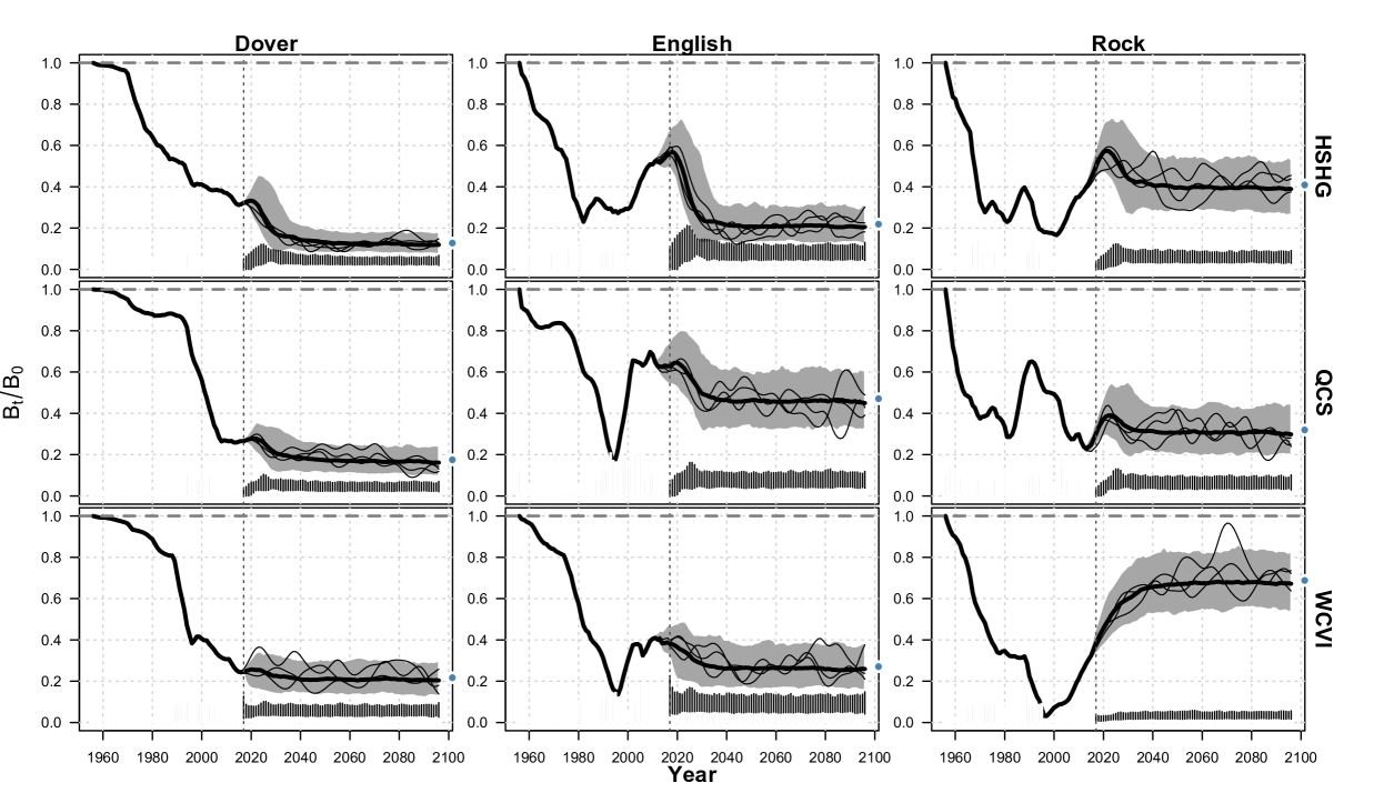
Figure 3: Spawning biomass depletion and relative catch simulation envelopes for all nine DER complex management units from the omniscient manager simulations. Median biomass is shown by the thick black line, with the grey region showing the central 95% of the distribution of spawning biomass, and thin black lines showing three randomly selected simulation replicates. Catch is shown as grey bars in the historical period, which represent median catch in the projection, with thin vertical line segments showing the central 95% of the catch distribution. The depletion level associated with the traditional single species optimal biomass $B_{MSY,SS}$ is shown as a dashed horizontal green line, while the depletion level associated with our derived complex level multi-species optimal yield is shown as a blue horizontal dashed line.

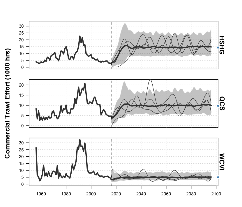
Figure 4: Commercial fishing effort simulation envelopes for each stock area. Historical and median simulated effort in the projection period are shown by a thicker black line, while the central 95% of the distribution of simulated effort is shown as grey shaded region in the projection period. Single simulation replicates in the projection period are shown as thinner black lines.

As expected, the omniscient manager was able to achieve the theoretical multi-species optimal yield in the presence of technical interactions (Figure 3, blue closed circle). Median biomass, catch, and fishing mortality reach the equilibrium after a transition period of about 20 years. During the transitionary period, effort is slowly ramped up in each area from the end of the historical period, stabilising around area-specific $E_{MSY}$ after about 12 years (Figure 4, blue closed circles).

The multi-species optimal effort for the complex results in overfishing Dover sole stocks between 53% and 92% of area-/single-species $B_{MSY}$ to increase fishery access to English and Rock sole. Despite this tendency toward overfishing Dover sole, very few optimal solutions risk severe overfishing of Dover sole below 40% of $B_{MSY}$, indicating that lost Dover sole yield from further overfishing relative to single-species optimal levels is not compensated by increased English and Rock sole yield (Table 5). The probability of being critically overfished in the period 2028 - 2037 was 0% for most stocks, with two Dover sole stocks having 3% (HSHG) and 1% (QCS).

Although DER stocks begin the simulations in an overall healthy state, the omniscient manager reduced fishing effort to near 0 in HSHG and QCS areas early in the projection period in some replicates (Figure 4, HSHG and QCS, 2016-2020). In these cases, anticipatory feedback control by the omniscient manager reduced fishing effort to avoid low spawning stock biomasses, thus and ensuring higher production in later time steps where recruitment process error deviations were sustained at low levels.

3.2 Assessment model performance

3.2.1 Catch loss

Hierarchical Multi-stock assessment models ranked highest, on average, under the Poor and Mod data quality scenarios (Table 6). Under the Poor data quality scenario, the Hierarchical model had the lowest cumulative absolute catch loss, on average, and ranked in the top three assessment methods for all stocks. As data quantity increased for the Mod scenario, the average absolute rank of the Hierarchical model degraded slightly, but still came first in average rankings. It was only under the Rich scenario that the Hierarchical model average rank fell to fourth place, although it still ranked above the Single-stock model.

Under the Rich data quality scenario, the Species Pooling and Total Aggregation methods ranked best, never ranking below fourth for all stocks (Table 6, Rich). As data was removed for the Mod data quality scenario, the average ranks of both Species Pooling and Total Aggregation methods degraded, placing them second and third. The Single-stock model had the worst average rank under all data-quality scenarios, with its worst performance observed under the Mod data quality scenario where it ranked 5th across all stocks.

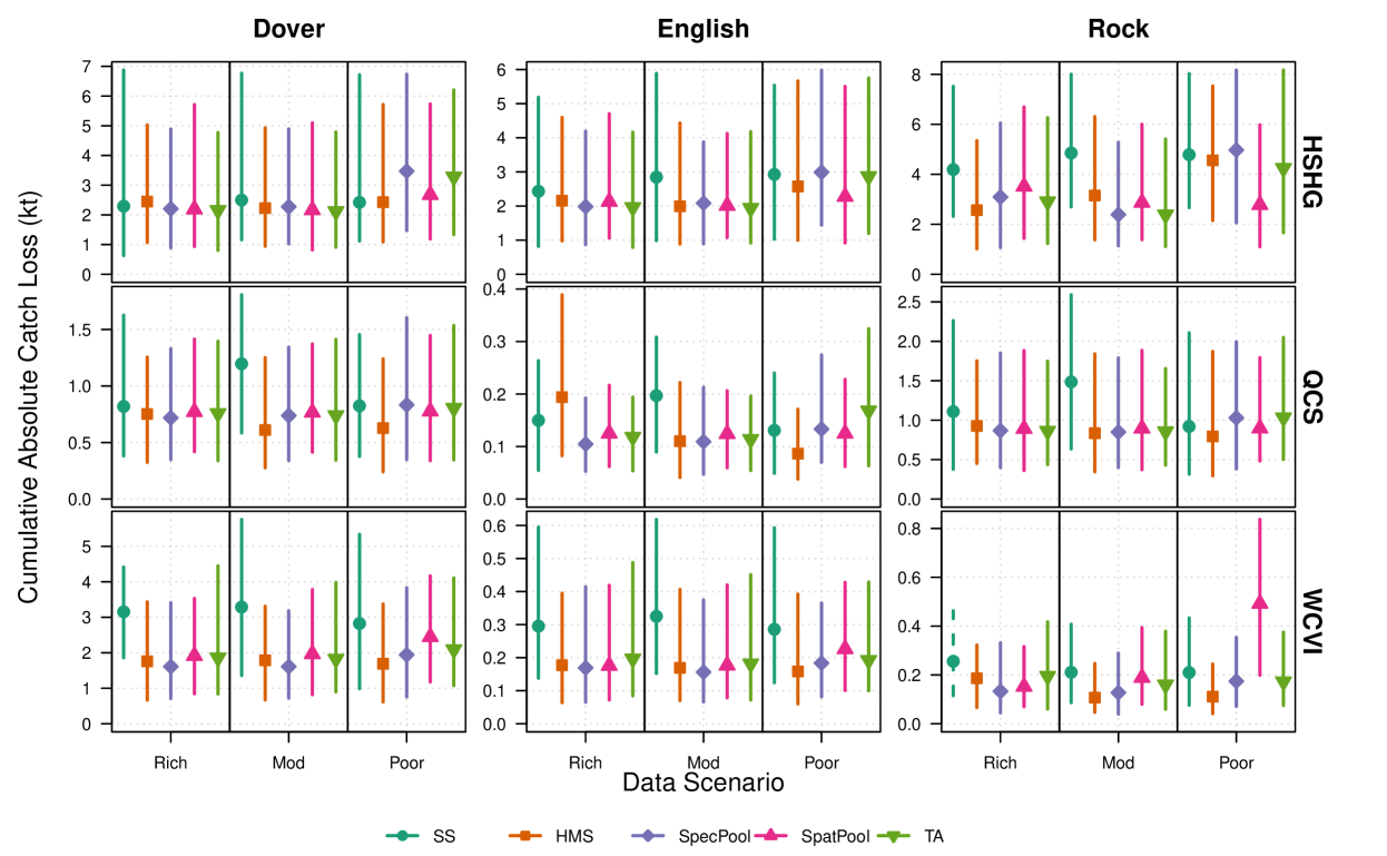
Figure 5: Distributions of cumulative absolute loss in catch (kt) for the projection years 2026 to 2036 under each assessment model and OM data scenario (x-axis labels). The points show the median loss, while line segments show the central 90% of cumulative loss distributions. Panels show the cumulative loss distributions by species (columns) and stocks (rows). Each assessment model point type and colour is shown in the legend at the bottom. Loss distributions for assessment models that couldn’t reach 100 replicates with satisfactory convergence are shown as a dashed line.

Cumulative catch loss distributions for the Hierarchical model and three data-pooling methods were fairly closely clustered for the Rich and Mod data quality scenarios for most stocks (Figure 5). Only the Single-stock model was qualitatively different, but this was not always the case (e.g., HSHG Dover, Figure 5). Relative performance of each method across data quality scenarios was stock dependent, with no consistent trends across scenarios and stocks.

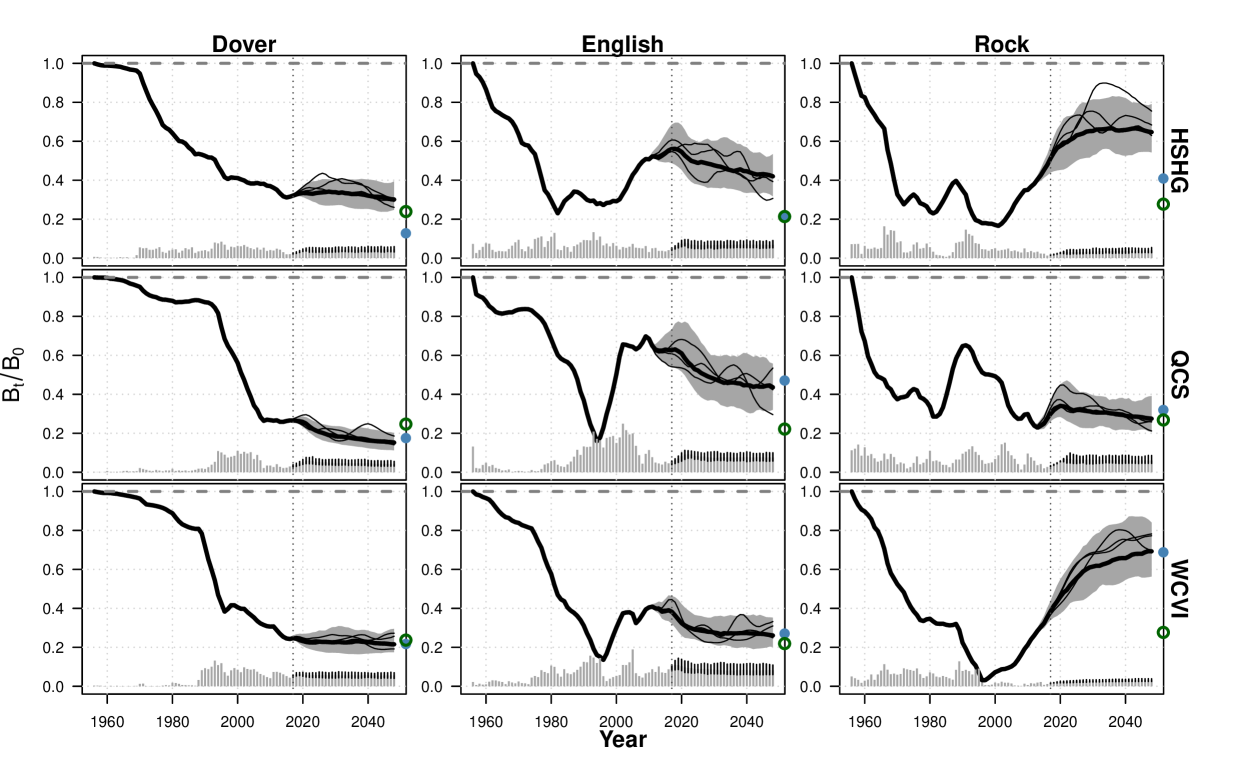
Figure 6: Spawning biomass depletion and relative catch simulation envelopes for all nine DER complex management units when assessed by the Hierarchical Multi-stock assessment model under the Poor data-quality scenario. Median biomass is shown by the thick black line, with the grey region showing the central 95% of the distribution of spawning biomass, and thin black lines showing three randomly selected simulation replicates. Catch is shown as grey bars in the historical period, which represent median catch in the projection, with thin vertical line segments showing the central 95% of the catch distribution. Coloured circles on the right hand vertical axis show the biomass depletion level associated with the multi-species (closed blue circle) and single-species (open green circle) maximum sustainable yield.

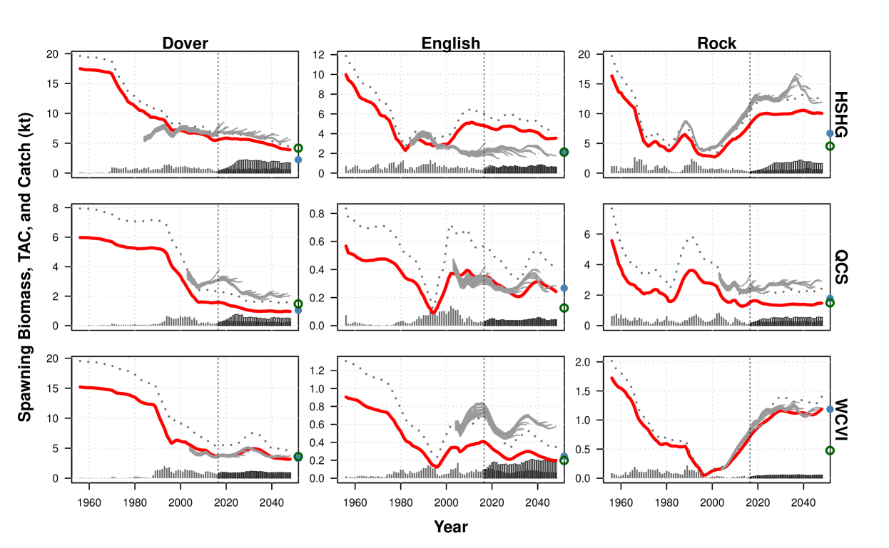
Figure 7: Operating model spawning stock biomass (red line), commercial trawl vulnerable biomass (grey dotted line), retrospective assesment model estimates of spawning stock biomass (thin grey/purple lines), and catch and TACs (grey bars) from the first simulation replicate in the Poor data-quality scenario and under the Hierarchical Multi-stock assessment model. Catch bars show realised catch in grey for the whole simulation period, and unfilled bars in the projection period show the difference between MP set TACs and realised catch. Coloured circles on the right hand vertical axis show the biomass level associated with the multi-species (closed blue circle) and single-species (open green circle) maximum sustainable yield.

Technical interactions had both a positive and negative effect on meeting the multi-species objectives and minimising catch loss. For example, over the course of the projection period, the Hierarchical Multi-stock model was able to bring median biomass levels close to the multi-species optimal level $B_{MSY,MS,s,p}$ for six out of the nine stocks under the Poor data quality scenario (Figure 6, blue dots). The three stocks that did not meet the multi-species optimal biomass were all in the HSHG area, indicating that technical interactions may have been a factor in the inability to meet the target harvest rates, choking off TACs for some species in HSHG. For the HSHG area, catch of Dover and Rock soles are choked by English sole TAC (Figure 7, HSHG, unfilled TAC bars), which is low relative to the target level because the Hierarchical assessment model viewed HSHG English sole as a larger and less productive stock than it truly was, resulting in a persistent negative bias in the stock assessment biomass. Furthermore, there is evidence that a large perturbation is needed to improve the assessment for HSHG English sole and overcome the choke effect, as the assessment model believes the TACs are appropriately scaled and biomass is approaching $B_{MSY,MS}$. For QCS and WCVI areas, all stocks were able to meet the target harvest objectives and minimise loss directly because technical interactions protected against overfishing. In QCS, English sole had close to unbiased assessments, and was able to limit catches for Dover and Rock soles despite large positive assessment errors for both (Figure 7, QCS). Similarly, WCVI English sole catch was choked by TACs for Dover and Rock sole, which both had unbiased assessments (Figure 7, WCVI).

3.2.2 Catch-Biomass trade-offs

Distributions of catch and biomass relative to $MSY_{MS}$ and $B_{MSY,MS}$, respectively, were produced for the time period $2028\leq t\leq 2037$ for each assessment model and Scenario combination. The medians of those relative catch and biomass distributions were visually compared to each other and to the central 95% of the omniscient manager’s trajectories over the same time period, to understand the biomass and catch trade-offs between different model choices, and to compare each model to the omniscient manager’s optimal solution.

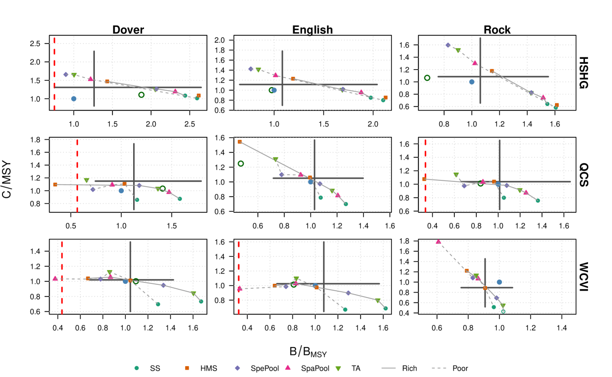
Figure 8: Tradeoff between catch and biomass during the 2028 - 2037 period implied by switching between different assessment models under Rich and Poor data-quality scenarios. Panels are gridded by species (columns) and stocks (rows), with biomass relative to $B_{MSY,MS,s,p}$ on the horizontal axis, and catch relative to $MSY_{MS,s,p}$ on the vertical axis. Distributions of biomass and catch under the omniscient manager are shown by the black crosshair, with points indicating optimal biomass and yield for single species maximum yield (open green circles) and multi-species maximum yield (closed blue circles). The biomass level at which a stock is critically overfished is shown as a vertical red dashed line. Coloured point symbols show median biomass and catch for over all replicates for different assessment models, with assessment models under the same data-quality scenario joined by a solid line (Rich) or dashed line (Poor).

As indicated in the loss rankings, the Hierarchical Multi-stock assessment model median biomass and catch between 2028 and 2037 came closest (i.e., smaller Euclidean distance) to the omniscient manager median levels under the Poor data quality scenario outside the HSHG area (Figure 8, compare points to the centre of the black crosshairs). Within HSHG, the Hierarchical model tended to underfish relative to the omniscient manager for the Poor data scenario, creating a large biomass surplus and the lowest catch next to the Single-stock model, while the Spatial Pooling method came closest to the omniscient manager for all three species.

Although the range of biomass-catch trade-offs are quite broad for each stock, the majority of Scenario/Assessment combinations lie inside the central 95% distributions of the omniscient manager (Figure 8, black crosshairs). Notable exceptions to this were (i) the Single-stock model under the Rich data quality scenario, (ii) the Hierarchical model in QCS under the Rich data quality scenario where Dover and Rock sole were both critically overfished, (iii) the Spatial Pooling method in WCVI under the Poor data quality scenario where Dover and English sole were critically overfished, and (iv) the Total Aggregation and Species Pooling methods under the Poor data quality scenario in QCS.

Catch-biomass trade-offs were approximately collinear under both Rich and Poor data quality scenarios for all HSHG stocks, QCS English sole, and WCVI Rock sole. For all these stocks except WCVI Rock sole, spawning biomass is well above both the single-species and multi-species optimal levels at the beginning of the projection period (e.g., Figure 6, compare biomass at the start of the projection period to green open and blue closed circles), meaning that the catch limits set by all methods were depleting a standing stock and benefited from its surplus production. Under these conditions, an increase in catch almost linearly caused a decrease in biomass as the compensatory effect of density dependence was minimal. A similar phenomenon explains the WCVI Rock sole collinearity, but there the biomass was growing from a starting point above the single-species $B_{MSY,SS}$ towards the multi-species optimal level $B_{MSY,MS}$, asymptotically approaching it as biomass equilibrates to a harvest rate well below the single species optimal rate $U_{MSY,SS}$.

Catch-biomass trade-offs in the HSHG area indicated that Hierarchical models performed more similar to the omniscient manager under the Rich data quality scenario (Figure 8, HSHG). In the same area, the Species Pooling method (ranked highest under the Rich scenario) produced median biomass between 140% and 210% of the multi-species optimal level (Figure 8, HSHS, Purple diamond), despite the superior performance with respect to catch loss for Dover and English soles (indicated by proximity to the horizontal median catch line).

As mentioned above, several stocks were pushed into a critically overfished state by different methods. The Hierarchical Multi-stock model (QCS, Rich data quality scenario) and Spatial Pooling method (WCVI, Poor data quality scenario) produced median biomass levels that were below 40% of $B_{MSY,SS}$ for two out of three species in each area (Figure 8, QCS and WCVI). These methods avoided pushing the QCS English and WCVI Rock soles, respectively, into critically overfished states thanks largely to their relatively low commercial catchability scalars. Low catchability means that their multi-species optimal biomass $B_{MSY,MS}$ was well above the single-species optimal biomass level $B_{MSY,SS}$, providing plenty of room to overshoot the optimal biomass level while still avoiding the critically overfished level. Even so, median biomass is still well outside the omniscient manager’s distribution for both stocks, with catches far above the omniscient manager’s median catch, ranging between 150% and 180% of maximum yield under multi-species $E_{MSY}$. Finally, Total Aggregation and Spatial Pooling assessment methods had higher than 10% probability of being below 40% of $B_{MSY,SS}$ under the Poor data scenario for (i) HSHG Dover sole (37 % Total Aggregation, 42% Species Pooling), (ii) QCS Dover sole (37 % Total Aggregation, 11% Species Pooling), (iii) HSHG English (12 % Total Aggregation, 11 % Species Pooling), and (iv) QCS Rock sole (11% Total Aggregation).

3.3 Sensitivity of results to prior standard deviations

We summarised average model sensitivities by fitting linear regressions to the distributions of median cumulative loss. To remove the effect of absolute catch scales on the regressions, median loss distributions were standardised across assessment models, stratified by species, stock-area, and data scenario. Regressions with positive slopes have increasing catch loss with increasing prior uncertainty, and negative or zero slopes indicate a decrease or no change in catch loss with increasing prior uncertainty.

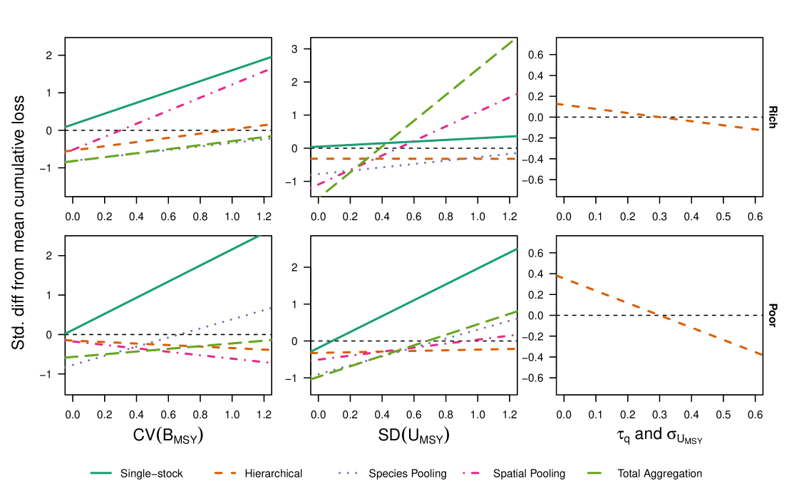
Figure 9: Regressions showing the average sensitivity of cumulative catch loss to the prior standard deviations under each assessment model (colours, line types) for the data-rich (left column) and data-poor (right column) scenarios. The horizontal axis on each plot shows the prior standard deviation (CV for $B_{MSY}$), while the vertical axis shows the standardised difference between median cumulative loss for an assessment model and the mean of median cumulative loss values over AMs, stratified by species and area. See the online version of the journal for a full colour version of the plot.

The Hierarchical Multi-stock model was least sensitive to increasing $B_{MSY}$ prior CVs in both Rich and Poor data quality scenarios. Cumulative catch loss actually decreased on average with increasing $B_{MSY}$ prior CVs when catch limits were set by the Hierarchical model under the Poor data quality scenario, decreasing by about 0.3 standard deviations over the range of CVs tested (Figure 9, left column, Poor). While cumulative catch loss from Hierarchical models increased on average with increasing $B_{MSY}$ prior CVs under the Rich data quality scenario, the slope of the regression line was the lowest among methods (equal with the Species Pooling and Total Aggregation methods), implying the least sensitivity to prior specifications.

Cumulative catch loss under the Hierarchical model was also insensitive to the complex mean $U_{MSY}$ hyperprior standard deviation, with zero slope regression lines under both Rich and Poor data quality scenarios over the range of tested log-normal prior SDs (Figure 9, middle column). The lack of sensitivity of the Hierarchical model to the $U_{MSY}$ hyperprior was partially because target harvest rates were based on theoretically optimal levels, and not estimated from the assessment model; however, this implies that the biomass estimates were also insensitive to the hyperprior standard deviation, which may be because the effect of the hyperprior was soaked up by the two levels of shrinkage priors between the complex mean and stock-specific estimates of $U_{MSY}$.

Hierarchical Multi-stock assessment models were more able to suitably scale catch limits to operating model biomass under relaxed catchability and $U_{MSY}$ hierarchical shrinkage priors. As $\sigma_{U_{MSY}}$ and $\tau_{q}$ increased from 0.1 to 0.5, average catch loss dropped by about 0.4 standard deviations under the Rich data quality scenario, and 0.8 standard deviations for the Poor data quality scenario (Figure 9, third column). Improvements stemmed from a change in assessment model errors in the HSHG area, in particular (Figures C.1, C.2, Appendix C). The change in assessment performance switched the choke species from English to Rock sole in HSHG, and while most assessments were biased and had strong retrospective patterns, the combination of higher catch limits and favourable technical interactions produced catches that were more closely aligned with the omniscient manager’s and the multi-species maximum yield.

As expected, cumulative catch loss increased with decreasing prior precision under all other assessment methods. The Single-stock model was most sensitive to $B_{MSY}$ CVs under both Rich and Poor data quality scenarios, and to $U_{MSY}$ log-normal SDs under the Poor data quality scenario, indicating that the single-stock model required the most prior knowledge for scaling biomass estimates correctly. The Total Aggregation and Spatial Pooling methods were most sensitive to the $U_{MSY}$ prior standard deviation, which may indicate a that the aggregate prior mean values we calculated for those assessment models were not well supported by the aggregated data.

4 Discussion

In this paper, we demonstrated that hierarchical stock assessment models may improve management performance in a data-limited, multi-species flatfish fishery. When available data quality was moderate or poor (indicated here by time-series length), biomass estimates from hierarchical stock assessment models resulted in catches that were closer to an omniscient manager’s optimal reference series compared to catch limits derived from single-stock and data-pooling assessment methods. Under high data quality scenarios, data-pooling methods outperformed hierarchical models, but the latter still outperformed single-stock assessment methods. Improved performance relative to single-stock models under lower data quality conditions is consistent with our previous study, where statistical performance of hierarchical multi-stock assessments improved with decreasing data quantity and quality (Johnson and Cox, 2018). This suggests that hierarchical assessment methods would generally be a better approach than conventional single-species methods under typical fisheries data quality conditions.

Our results arise from models that are necessarily a simplification of the real stock-management system. The harvest rules applied to DER complex species were relatively simple and may require more detail or complexity for practical applications. First, the harvest rules were all constant target harvest rates, which do not include precautionary “ramping-down” of catch towards a limit biomass level (DFO, 2006; Cox et al., 2013). Including a ramped harvest rule may have reduced the probability of some stocks being critically overfished in some cases, but probably at some further cost of choke effects. Second, catch limits for the simulated DER complex were set based on fixed target harvest rates that were derived a priori from multi-species yield curves, and not estimated as part of the assessment models that we tested. Incorporating multi-species yield curve calculations based on assessment model ouput into the harvest decision would be simple to do, but would require either a model of increased complexity to link fishing effort to single-species yield, or an extra assumption linking effort to surplus production model yield calculations, which would likely increase assessment model errors. Finally, the TAC allocation model for data-pooled methods was only one example from a large set of potential options. Understanding the relative risks of data-pooling would require testing alternative allocation methods, which was beyond the scope of this paper.

We only considered multi-species technical interactions, which although an important part of exploited system dynamics, are not the entire story. Although there is limited evidence for ecological interactions among DER complex species (Pikitch, 1987; Wakefield, 1984), what does exist may influence the multi-species yield relationship with fishing effort or, as with technical interactions, inhibit the ability of the management system to meet target catch levels. For example, individual survival or growth may change in response to varied fishing pressure due to unmodeled linkages (Collie and Gislason, 2001). Yet, including such ecological interactions would imply a highly data rich scenario, which is counter to our focus on data-limited, multi-species fisheries. Furthermore, accounting for potential ecological interactions would require multiple OMs to test performance against a range of plausible hypotheses since ecological uncertainties are much broader in complexity and scope than technical interactions alone. Nevertheless, future work combining technical interactions with minimum realistic models for ecological interactions could help determine the extent to which assessment approaches affect these more complex multi-species fisheries outcomes (Punt and Butterworth, 1995). For example, while diet overlap between the three species is small off the coast of Oregon, the major Rock sole prey was recently settled pleuronectiform fishes, which may include Dover and English sole young and therefore shift the complex equilibrium as fishing pressure is applied, reducing predation mortality for Dover and English sole and prey availability for Rock sole (Wakefield, 1984; Collie and Gislason, 2001).

Our effort model applied to the DER complex was also a simplification of reality, where effort was limited only by the TACs in each area. Limiting by TACs was intended to reflect the management of the real BC groundfish fishery in which harvester decisions drive TAC utilisation among target species (via increasing catchability; Punt et al., 2011a), and non-target or choke species (via decreasing catchability; Branch and Hilborn, 2008). Changing catchability for targeting or avoidance could be simulated as a random walk in the projections, with correlation and variance based on the historical period, or perhaps simulated via some economic sub-model that accounted for ex-vessel prices and variable fishing costs. These economic factors could affect targeting and avoidance behaviour among species (Punt et al., 2011a, 2020), as well as effort allocation among stock-areas (Hilborn and Walters, 1987; Walters and Bonfil, 1999); however, it is not clear that our median results would be significantly different given the potential magnitude of assessment model errors in data-limited scenarios. Impacts of a detailed effort dynamics sub-model would probably be more important in more extreme data-limited scenarios that relied solely on fishery CPUE as an index of abundance. In fact, it would be interesting to determine whether the hierarchical information-sharing approach would exacerbate assessment model errors in such a (common) context where fishery CPUE is the main abundance index.

Despite the limitations above, our results indicate that even in fisheries with long time series of catch and effort data, hierarchical multi-species assessment models may be preferable over typical single-species methods. The poor performance of the single-species models in all scenarios highlights the difference between data-rich (i.e., a higher quantity of data) and information-rich (i.e., data with higher statistical power) fisheries. The data-rich scenario differed from data-moderate and data-poor scenarios by the inclusion of a historical series of fishery dependent CPUE, which was quite noisy and subject to the effects of changing harvester behaviour like targeting (variable catchability), and therefore, additional historical CPUE data had little effect on cumulative catch loss under the single-species models. In contrast, the data-pooling procedures all ranked higher than single-species and multi-species models under the data-rich scenario, as they were able to leverage additional statistical power from the historical CPUE by effectively increasing the sample size through data aggregation. The superior performance of the hierarchical model over the single-species model under the data-rich scenario indicate that shared priors partially compensate for low statistical power, but not as much as data-pooling.

Although the data-pooled methods performed better under the rich scenario, they were more sensitive to priors, so those results may be optimistically biased in all scenarios. Data-pooled observation errors were simulated as independent of the observation errors in the component indices, using the average standard deviation of the components. If aggregate indices pooled errors from each component index, then the resulting observation error variance would be additive in the components, especially if those errors were positively correlated, which may be the case under a common survey or fishery.

A dual effect of control was observed under catch limits set by the hierarchical models in the data-poor scenario, in which lower contrast in assessment model outputs reduced the statistical power of assessment model data, sacrificing long term adaptability of the management system in favour of short term stability in catch. Moreover, there was limited evidence that adaptive learning was facilitated through the shared hierarchical prior distributions (Collie and Walters, 1991). Uninformative catch series resulting from a lack of large perturbations (sometimes caused by large catch errors) resulted in hierarchical multi-species assessment model estimates that viewed HSHG English sole as a larger and less productive stock, causing negatively biased assessment estimates of biomass to approach the multi-species $B_{MSY,MS}$ value for that stock, and indicating that the assessments believed the TACs were appropriately scaled to the target harvest rates. Relaxing hierarchical prior standard deviations in the sensitivity analysis removed this persistent bias and all stocks approached biomass levels associated with multi-species maximum yield; however, information sharing was not wholly responsible for the improved behaviour, which appeared to also rely on a favourable combination of assessment errors and technical interactions as in the other stock areas. Adaptive learning catalysts like large stock perturbations may have been limited by a low recruitment process error standard deviation of $\sigma_{s,p}=.4$ in DER complex simulations, which was required for fitting the DER complex OM to data. Future work could relax this assumption to test whether perturbations stemming from higher recruitment variability would improve adaptive learning of hierarchical assessment methods (Walters, 1986).

We showed that choke effects are not a uniformly negative outcome for multi-species fisheries, and may indicate a mismatch between the target harvest rate and optimal complex yield. The usual assumption is that choke species restrict access to fishing grounds, decreasing profitability through lost yield of target species, and higher quota prices for choke species (Mortensen et al., 2018); however, we found that choke species sometimes prevented overfishing when TACs for the non-choke species were set too high, allowing harvest strategies to meet multi-species objectives despite large assessment errors for individual species in the complex. In reality, choke effects would likely be lessened by changing species catchability via harvester targeting and avoidance, creating a more complex relationship between effort and complex yield; but, the existence of a choke species would still indicate a mismatch between an individual species TAC and the optimal exploitation level for the multi-species complex.

4.1 Conclusion

Hierarchical multi-species assessment models can out-perform single-species assessment models in meeting multi-species harvest objectives across data-rich, data-moderate, and data-poor scenarios. As expected, biomass estimation performance of hierarchical models improved relative to other methods as data quantity was reduced, and - as hoped - this translated into improved management performance across the multi-species flatfish fishery. We therefore recommend that assessment and management of multi-species fisheries include technical interactions when designing harvest strategies and management procedures aimed at achieving strategic objectives. Otherwise, error-prone single-species approaches may give a misleading picture of the expected performance of multi-species fishery management.

5 Acknowledgements

Funding for this research was provided by a Mitacs Cluster Grant to S.P. Cox in collaboration with the Canadian Groundfish Research and Conservation Society, Wild Canadian Sablefish, and the Pacific Halibut Management Association. We thank S. Anderson and M. Surry at the Fisheries and Oceans, Canada Pacific Biological Station for fulfilling data requests. Further support for S.P.C. and S.D.N.J. wass provided by an NSERC Discovery Grant to S.P. Cox.

6 Tables

Table 1: Fishery dependent and independent indices of biomass available for stock assessments of DER complex species.

Series	Extent	Description
Historical Commercial	1976 - 1995	Historical period commercial CPUE
Modern Commercial	1996 - 2016	Modern period commercial CPUE
HS Assemblage	1984 - 2002	Hecate Strait Assemblage trawl survey biomass index, biennial
Synoptic	2003 - 2016	Multi-species Synoptic trawl survey biomass index, biennial

Table 2: Unfished biomas $B_{0}$, single-species MSY based reference points $B_{MSY,SS}$ and $U_{MSY,SS}$, stock status as absolute biomass in 2016 $B_{2016}$, depletion relative to single-species optimal biomass $B_{2016}/B_{MSY,SS}$, and commercial trawl catchability scalar $q^{F}$ for all DER complex stocks in 2016. Biomass quantities are given in kilotonnes, and depletion and harvest rates are unitless.

	Single-species Reference Points			Stock Status		Comm. Catchability
Stock	$B_{0}$	$B_{MSY,SS}$	$U_{MSY,SS}$	$B_{2016}$	$B_{2016}/B_{MSY,SS}$	$q^{F}$
Dover sole
HSHG	17.50	6.06	0.17	6.06	1.00	0.022
QCS	5.98	1.99	0.15	1.74	0.88	0.017
WCVI	15.20	5.03	0.19	4.05	0.81	0.039
English sole
HSHG	9.98	3.42	0.31	5.95	1.74	0.024
QCS	0.57	0.19	0.29	0.38	2.04	0.011
WCVI	0.90	0.30	0.29	0.38	1.26	0.042
Rock sole
HSHG	16.35	5.75	0.23	8.40	1.46	0.009
QCS	5.57	1.90	0.21	1.63	0.86	0.014
WCVI	1.72	0.63	0.23	0.68	1.09	0.009

Table 3: Prior distributions used for each assessment model. For single stock and hierarchical multi-stock assesssment models, $s_{f}$ is 1 for commercial indices, and 0.5 for survey indices.

Prior

Totally aggregated AM

$B_{MSY}\sim N(\mu_{B_{MSY}},0.2\cdot\mu_{B_{MSY}})$

$\log U_{MSY}\sim N(\mu_{\log U_{MSY}},0.4)$

$\log q_{f}\sim N(\mu_{\log q_{f}},1.0)$

Species-Pooled AM

$B_{MSY,p}\sim N(\mu_{B_{MSY,p}},0.2\cdot\mu_{B_{MSY,p}})$

$\log U_{MSY,p}\sim N(\mu_{\log U_{MSY,p}},0.4)$

$\log q_{p,f}\sim N(\mu_{\log q_{p,f}},1.0)$

Spatial-Pooled AM

$B_{MSY,s}\sim N(\mu_{B_{MSY,s}},0.2\cdot\mu_{B_{MSY,s}})$

$\log U_{MSY,s}\sim N(\mu_{\log U_{MSY,s}},0.4)$

$\log q_{s,f}\sim N(\mu_{\log q_{s,f}},1.0)$

Single-stock AM

$B_{MSY,s,p}\sim N(\mu_{B_{MSY}},0.1\cdot\mu_{B_{MSY}})$

$\log U_{MSY,s,p}\sim N(\mu_{\log U_{MSY}},0.1)$

$\log q_{s,p,f}\sim N(\mu_{\log q_{s,p,f}},s_{f})$

Hierarchical multi-stock AM

$B_{MSY,s,p}\sim N(\mu_{B_{MSY}},0.2\cdot\mu_{B_{MSY}})$

$\log U_{MSY,s,p}\sim N(\log\overline{U}_{MSY,s},\sigma_{U_{MSY}})$

$\log\overline{U}_{MSY,s}\sim N(\log\overline{U}_{MSY},\sigma_{U_{MSY}})$

$\log\overline{U}_{MSY}\sim N(\mu_{\log U_{MSY}},0.4)$

$\log q_{s,p,f}\sim N(\log\overline{q}_{s,f},\tau_{q})$

$\log\overline{q}_{s,f}\sim N(\mu_{\log q_{s,f}},s_{f})$

All AMs

$\zeta_{s,p,t}\sim N(0,0.05)$

Table 4: Summary of sensitivity analyses, showing the total number of experiments, the factor being varied, the levels of that factor, and the data scenarios and AMs included in the analysis.

N	Factor	Levels	Scenarios	AMs
30	$B_{MSY}$ prior CV	$0.1,0.5,1.0$	Rich, Poor	All
30	$U_{MSY}$ prior SD	$0.1,0.5,1.0$	Rich, Poor	All
6	$\tau_{q}$, $\sigma_{U_{MSY}}$	$0.1,0.2,.5$	Rich, Poor	Hierarchical only

Table 5: Probability of being overfished and experiencing overfishing with respect to single-species reference points, and catching less than the historical miniumum during the time period 2028 - 2037 for all nine DER complex stocks when managed by the omniscient manager.

	Prob. of being overfished		Prob. of overfishing		Prob. of low catch
Stock	$P(B_{t}<.4B_{MSY,SS})$	$P(B_{t}<.8B_{MSY,SS})$	$P(C_{t}>MSY_{SS})$	$P(F_{t}>F_{MSY,SS})$	$P(C_{t}<\min C_{1951:2016})$
Dover sole
HSHG	0.03	0.70	0.74	0.97	0
QCS	0.01	0.46	0.66	0.86	0
WCVI	0.00	0.23	0.54	0.63	0
English sole
HSHG	0.00	0.12	0.64	0.49	0
QCS	0.00	0.00	0.24	0.00	0
WCVI	0.00	0.03	0.53	0.23	0
Rock sole
HSHG	0.00	0.01	0.50	0.06	0
QCS	0.00	0.04	0.53	0.29	0
WCVI	0.00	0.00	0.01	0.00	0

Table 6: Summary of AM rankings with respect to cumulative absolute catch loss between 2026 and 2035 under each scenario. The rank column shows the average rank of the AMs over all species/areas, and the range of that distribution in parentheses. AMs are ordered by mean rank within a scenario.

AM	Average Loss Rank (range)
Rich
Species Pooling	1.67 (1, 3)
Total Aggregation	2.33 (1, 4)
Spatial Pooling	3.00 (2, 4)
Hierarchical Multi-stock	3.22 (1, 5)
Single Stock	4.78 (4, 5)
Mod
Hierarchical Multi-stock	2.00 (1, 4)
Species Pooling	2.11 (1, 4)
Total Aggregation	2.44 (1, 4)
Spatial Pooling	3.44 (2, 4)
Single Stock	5.00 (5, 5)
Poor
Hierarchical Multi-stock	1.44 (1, 3)
Spatial Pooling	2.67 (1, 5)
Total Aggregation	3.33 (2, 5)
Single Stock	3.67 (1, 5)
Species Pooling	3.89 (2, 5)

7 Figures

Appendix A The operating model

The operating model was a standard age- and sex-structured operating model, with additional structure for multi-species and multi-stock population dynamics. DER complex species and stocks were simulated assuming no ecological interactions or movement between areas. The lack of movement may be unrealistic, especially for Dover Sole given their extent, but this is how the the DER complex stocks are currently managed in practice. The lack of ecological interactions is more realistic for Dover and English soles, as although both species are benthophagus, there is evidence that they belong to different feeding guilds (Pikitch, 1987).

DER complex abundance $N_{a,x,s,p,t}$ for age $a$, sex $x$, species $s$ and stock $p$ at the start of year $t$ was given by

$$N_{a,x,s,p,t}=\left\{\begin{array}[]{ll}0.5R_{s,p,t}&a=1,\\ N_{a-1,x,s,p,t-1}\cdot e^{-Z_{a-1,x,s,p,t-1}}&1<a<A,\\ N_{a-1,x,s,p,t-1}\cdot e^{-Z_{a-1,x,s,p,t-1}}+N_{a,x,s,p,t-1}\cdot e^{-Z_{a,x,s,p,t-1}}&a=A_{s},\end{array}\right.$$

where $R_{t}$ is age-1 recruitment in year $t$, $Z_{a,x,s,p,t}$ is the instantaneous total mortality rate, and $A_{s}$ is the plus group age for species $s$.

Numbers-at-age were scaled to biomass-at-age by sex/species/area- specific weight-at-age. Weight-at-age was an allometric function of length-at-age

$$w_{a,x,s,p}=\alpha_{x,s,p}\cdot L_{a,x,s,p}^{\beta_{x,s,p}}$$

where $\alpha_{x,s,p}$ scaled between cm and kg, $\beta_{x,s,p}$ determined the rate of allometric growth, and $L_{a,x,s,p}$ was the length in cm of a fish of age $a$, sex $x$, species $s$ and stock $p$. Length-at-age was given by the following Schnute formulation of the von-Bertalanffy growth curve (Schnute, 1981; Francis et al., 2016)

$$L_{a}=\overline{L}_{A_{1}}-(\overline{L}_{A_{2}}-\overline{L}_{A_{1}})\cdot\left(\frac{e^{-kA_{1}}-e^{-ka})}{e^{-kA_{1}}-e^{-kA_{2}}}\right)$$

where $A_{1}$ and $A_{2}$ are well spaced reference ages, $\overline{L}_{A_{1}}$ and $\overline{L}_{A_{2}}$ are the mean lengths in cm of fish at ages $A_{1}$ and $A_{2}$, and $k$ is the growth coefficient. Note that in the growth model we dropped the sex, species and stock subscripts for concision.

The maturity-at-age ogive was modelled as a logistic function

$$m_{a,s,p}=\left(1+e^{-\frac{\ln 19(a-a_{50,s,p}^{mat})}{a_{95,s,p}^{mat}-a_{50,x,s,p}^{mat}}}\right)^{-1},$$

where $m_{a,s,p}$ was the proportion of age-$a$ female fish of species $s$ in stock $p$ that were mature, and $a_{50,s,p}^{mat}$ and $a_{95,s,p}^{mat}$ are the ages at which 50% and 95% of fish of age-$a$, species $s$ and stock $p$ were mature.

Female spawning stock biomass was calculated as

$$B_{s,p,t}=\sum_{a}N_{a,x^{\prime},s,p,t}m_{a,s,p}w_{a,x^{\prime},s,p},$$

where $x^{\prime}$ denotes female fish only. Spawning stock biomass was used to calculate expected Beverton-Holt recruitment, which then had recruitment process errors applied

$$R_{s,p,t+1}=\frac{R_{s,p,0}\cdot 4h_{s,p}\cdot B_{s,p,t}}{B_{s,p,0}\cdot(1-h_{s,p})+(5h_{s,p}-1)\cdot B_{s,p,t}}\cdot e^{\epsilon_{s,p,t+1}-0.5\sigma_{R,s,p}^{2}},$$

where $R_{s,p,0}$ is unfished equilibrium recruitment, $B_{s,p,t}$ is the spawning stock biomass at time $t$, $B_{s,p,0}$ is unfished spawning stock biomasss, $h_{s,p}$ is stock-recruit steepness (average proportion of $R_{s,p,0}$ produced when $B_{s,p,t}=.2B_{s,p,0}$), and $\epsilon_{s,p,t}$ is the recruitment process error with standard deviation $\sigma_{R,s,p}$.

The operating model was initialised in 1956 at unfished equilibrium for all species $s$ and areas $p$, with numbers-at-age in 1956 given by

$$N_{a,x,s,p,1956}=\left\{\begin{array}[]{ll}0.5R_{s,p,0}&a=1,\\ N_{a-1,x,s,p,1956}\cdot e^{-M_{x,s,p}}&1<a<A,\\ N_{a-1,x,s,p,1956}\cdot\frac{e^{-M_{x,s,p}}}{1-e^{-M_{x,s,p}}}&a=A,\end{array}\right.$$

Fishery removals were assumed to be continuous throughout the year, with fishing mortality-at-age

$$F_{a,x,s,p,f,t}=S_{a,x,s,p,f}\cdot F_{s,p,f,t},$$

where $F_{s,p,f,t}$ is the fully selected fishing mortality rate for fleet $f$ at time $t$, and $S_{a,x,s,p,f}$ is the selectivity-at-age $a$ for sex $x$ in species $s$ and area $p$ by fleet $f$. Selectivity-at -age was modeled as a logistic function of length-at-age

$$S_{a}=\left(1+\exp\left(\frac{-\ln 19(L_{a}-l^{sel}_{50})}{l^{sel}_{95}-l^{sel}_{50}}\right)\right)^{-1},$$

where $L_{a}$ is length-at-age, defined above, and $l^{sel}_{50}$ and $l^{sel}_{95}$ are the length-at-50% and length-at-95% selectivity, respectively; stock, species and fleet subscripts are left off for concision. Catch-at-age was then found via the Baranov catch equation

$$C_{a,x,s,p,f,t}=(1-e^{-Z_{a,x,s,p,f,t}})\cdot N_{a,x,s,p,t}w_{a,x,s,p}\frac{F_{a,x,s,p,f,t}}{Z_{a,x,s,p,f,t}},$$

where total mortality-at-age is defined as

$$Z_{a,x,s,p,f,t}=M_{x,s,p}+S_{a,x,s,p,f}\cdot F_{a,x,s,p,f,t}.$$

A.1 Observation error standard deviations

Operating model observation error standard deviations were derived from estimates from fitting a hierarchical age-structured model to DER complex data [Johnson and Cox, in prep]. To improve convergence in the simulations, we multipled all estimates by $0.3$ to improve observation model precision (multiplier found by trial and error).

Table 1: Log-normal observation error standard deviations for all DER complex biomass indices

	Observation Error SD
Stock	Historical	Modern	HS Ass.	Syn
Dover sole
HSHG	0.174	0.158	0.328	0.138
QCS	0.187	0.155		0.149
WCVI	0.221	0.161		0.092
English sole
HSHG	0.170	0.163	0.255	0.191
QCS	0.225	0.171		0.203
WCVI	0.216	0.174		0.136
Rock sole
HSHG	0.164	0.161	0.254	0.187
QCS	0.176	0.184		0.205
WCVI	0.198	0.233		0.214

Appendix B Omniscient Manager Optimisation

We defined penalty functions so that inside their respective desired regions the penalty was zero, and otherwise the penalty grew as a cubic function of distance from the desired region. For example, a penalty designed to keep a measurement $x$ above a the desired region boundary $\epsilon$ is of the form

$$\mathcal{P}(x,\epsilon)=\left\{\begin{array}[]{ll}0&x\geq\epsilon,\\ |x-\epsilon|^{3}&x<epsilon.\\ \end{array}\right.$$ (24)

This form has a several advantages over simple linear penalties, or a logarithmic barrier penalty (Srinivasan et al., 2008). First, the cubic softens the boundary threshold $\epsilon$, effectively allowing a crossover if doing so favours another portion of the objective function. Second, unlike lower degree polynomials, cubic functions remain closer to the $x$-axis when $|x-\epsilon|<1$. Third, zero penalty within in the desirable region stops the objective function from favouring regions far from the boundaries of penalty functions. In contrast, a logarithmic function would favour overly conservative effort series to keep biomass far from a lower depletion boundary. Finally, the cubic penalty function and its first two derivatives are continuous at every point $x$, allowing for fast derivative-based optimisation methods.

We used a cubic spline of effort in each area to reduce the number of free parameters in the optimisation. For each area, 9 knot points were distributed across the full 40 year projection, making them spaced by 5 years. We padded the omniscient manager simulations by an extra eight years over the stochastic simulations to avoid any possible end effects of the spline entering the performance metric calculations. Effort splines were constrained to be between 0 and 120 times the operating model $E_{MSY,p}$, by replacing any value outside that range with the closest value inside the range (i.e. negative values by zero, large values by $120E_{MSY_{p}}$).

Appendix C Hierarchical model performance under relaxed shrinkage prior SDs

Figure 1: Spawning biomass depletion and relative catch simulation envelopes for all nine DER complex management units when assessed by the hierarchical multi-stock asssessment model under the Poor OM data quality scenario, when hierarchical shrinkage prior SDs were $\sigma_{U_{MSY}}=\tau_{q}=0.5$. Median biomass is shown by the thick black line, with the grey region showing the central 95% of the distribution of spawning biomass, and thin black lines showing three randomly selected simulation replicates. Catch is shown as grey bars in the historical period, which represent median catch in the projection, with thin vertical line segments showing the central 95% of the catch distribution. Coloured circles on the right hand vertical axis show the biomass depletion level associated with the multi-species (closed blue circle) and single-species (open green circle) maximum sustainable yield.

References

- Appeldoorn (1996) Richard S Appeldoorn. Model and method in reef fishery assessment. In Reef fisheries, pages 219–248. Springer, 1996.
- Baudron and Fernandes (2015) Alan R Baudron and Paul G Fernandes. Adverse consequences of stock recovery: European hake, a new “choke” species under a discard ban? Fish and Fisheries, 16(4):563–575, 2015. doi: 10.1111/faf.12079. URL https://doi.org/10.1111/faf.12079.
- Benson et al. (2015) Ashleen J Benson, Sean P Cox, and Jaclyn S Cleary. Evaluating the conservation risks of aggregate harvest management in a spatially-structured herring fishery. Fisheries Research, 167:101–113, 2015.
- Branch and Hilborn (2008) Trevor A Branch and Ray Hilborn. Matching catches to quotas in a multispecies trawl fishery: targeting and avoidance behavior under individual transferable quotas. Canadian Journal of Fisheries and Aquatic Sciences, 65(7):1435–1446, 2008. doi: 10.1139/F08-065. URL https://doi.org/10.1139/F08-065.
- Collie and Gislason (2001) Jeremy S Collie and Henrik Gislason. Biological reference points for fish stocks in a multispecies context. Canadian Journal of Fisheries and Aquatic Sciences, 58(11):2167–2176, 2001. doi: 10.1139/f01-158. URL https://doi.org/10.1139/f01-158.
- Collie and Walters (1991) Jeremy S Collie and Carl J Walters. Adaptive management of spatially replicated groundfish populations. Canadian Journal of Fisheries and Aquatic Sciences, 48(7):1273–1284, 1991. doi: 10.1139/f91-153. URL https://doi.org/10.1139/f91-153.
- Cox and Kronlund (2008) Sean P Cox and Allen Robert Kronlund. Practical stakeholder-driven harvest policies for groundfish fisheries in British Columbia, Canada. Fisheries Research, 94(3):224–237, 2008. doi: 10.1016/j.fishres.2008.05.006. URL https://doi.org/10.1016/j.fishres.2008.05.006.
- Cox et al. (2013) Sean P Cox, Allen R Kronlund, and Ashleen J Benson. The roles of biological reference points and operational control points in management procedures for the Sablefish (Anoplopoma fimbria) fishery in British Columbia, Canada. Environmental Conservation, 40(4):318–328, 2013. doi: 10.1017/S0376892913000271. URL https://doi.org/10.1017/S0376892913000271.
- de la Mare (1998) William K de la Mare. Tidier fisheries management requires a new MOP (management-oriented paradigm). Reviews in Fish Biology and Fisheries, 8(3):349–356, 1998. doi: 10.1023/A:1008819416162. URL https://doi.org/10.1023/A:1008819416162.
- DeMartini (2019) Edward E DeMartini. Hazards of managing disparate species as a pooled complex: A general problem illustrated by two contrasting examples from hawaii. Fish and Fisheries, 20(6):1246–1259, 2019.
- DFO (2006) DFO. A Harvest Strategy Compliant with the Precautionary Approach. Technical Report 2006/023, DFO Can. Sci. Advis. Rep., 2006.
- Fisheries and Oceans, Canada (2015) Fisheries and Oceans, Canada. Pacific Region Integrated Fisheries Management Plan: Groundfish, 2015.
- Francis et al. (2016) RIC Chris Francis, Alexandre M Aires-da Silva, Mark N Maunder, Kurt M Schaefer, and Daniel W Fuller. Estimating fish growth for stock assessments using both age–length and tagging-increment data. Fisheries research, 180:113–118, 2016.
- Gaichas et al. (2012) Sarah Gaichas, Robert Gamble, Michael Fogarty, Hugues Benoît, Tim Essington, Caihong Fu, Mariano Koen-Alonso, and Jason Link. Assembly rules for aggregate-species production models: simulations in support of management strategy evaluation. Marine Ecology Progress Series, 459:275–292, 2012. doi: 10.3354/meps09650. URL https://doi.org/10.3354/meps09650.
- Gislason (1999) Henrik Gislason. Single and multispecies reference points for baltic fish stocks. ICES Journal of Marine Science, 56(5):571–583, 1999. doi: 10.1006/jmsc.1999.0492. URL https://doi.org/10.1006/jmsc.1999.0492.
- Hilborn and Walters (1987) Ray Hilborn and Carl J Walters. A general model for simulation of stock and fleet dynamics in spatially heterogeneous fisheries. Canadian Journal of Fisheries and Aquatic Sciences, 44(7):1366–1369, 1987. doi: 10.1139/f87-163. URL https://doi.org/10.1139/f87-163.
- Hilborn and Walters (1992) Ray Hilborn and Carl J Walters. Quantitative Fisheries Stock Assessment: Choice, Dynamics and Uncertainty/Book and Disk. Springer Science & Business Media, 1992.
- Jiao et al. (2009) Yan Jiao, Christopher Hayes, and Enric Cortés. Hierarchical Bayesian approach for population dynamics modelling of fish complexes without species-specific data. ICES Journal of Marine Science: Journal du Conseil, 66(2):367–377, 2009. doi: 10.1093/icesjms/fsn162. URL https://doi.org/10.1093/icesjms/fsn162.
- Jiao et al. (2011) Yan Jiao, Enric Cortés, Kate Andrews, and Feng Guo. Poor-data and data-poor species stock assessment using a bayesian hierarchical approach. Ecological Applications, 21(7):2691–2708, 2011. doi: 10.1890/10-0526.1. URL https://doi.org/10.1890/10-0526.1.
- Johnson and Cox (2018) Samuel D N Johnson and Sean P Cox. Evaluating the role of data quality when sharing information in hierarchical multi-stock assessment models, with an application to dover sole. Can. J. Fish. Aquat. Sci, 2018. doi: 10.1139/cjfas-2018-0048. URL https://doi.org/10.1139/cjfas-2018-0048.
- Kempf et al. (2016) Alexander Kempf, John Mumford, Polina Levontin, Adrian Leach, Ayoe Hoff, Katell G Hamon, Heleen Bartelings, Morten Vinther, Moritz Staebler, Jan Jaap Poos, et al. The MSY concept in a multi-objective fisheries environment–Lessons from the North Sea. Marine Policy, 69:146–158, 2016. doi: 10.1016/j.marpol.2016.04.012. URL https://doi.org/10.1016/j.marpol.2016.04.012.
- Martell et al. (2008) Steven JD Martell, Carl J Walters, and Ray Hilborn. Retrospective analysis of harvest management performance for bristol bay and fraser river sockeye salmon (oncorhynchus nerka). Canadian Journal of Fisheries and Aquatic Sciences, 65(3):409–424, 2008. doi: 10.1139/f07-170. URL https://doi.org/10.1139/f07-170.
- Maunder and Piner (2015) Mark N Maunder and Kevin R Piner. Contemporary fisheries stock assessment: many issues still remain. ICES Journal of Marine Science, 72(1):7–18, 2015.
- Mortensen et al. (2018) Lars O Mortensen, Clara Ulrich, Jan Hansen, and Rasmus Hald. Identifying choke species challenges for an individual demersal trawler in the north sea, lessons from conversations and data analysis. Marine Policy, 87:1–11, 2018. doi: 10.1016/j.marpol.2017.09.031. URL https://doi.org/10.1016/j.marpol.2017.09.031.
- Ono et al. (2017) Kotaro Ono, Alan C Haynie, Anne B Hollowed, James N Ianelli, Carey R McGilliard, and André E Punt. Management strategy analysis for multispecies fisheries, including technical interactions and human behavior in modelling management decisions and fishing. Canadian Journal of Fisheries and Aquatic Sciences, (999):1–18, 2017. doi: 10.1139/cjfas-2017-0135. URL https://doi.org/10.1139/cjfas-2017-0135.
- Pella and Tomlinson (1969) Jerome J Pella and Patrick K Tomlinson. A generalized stock production model. Inter-American Tropical Tuna Commission Bulletin, 13(3):416–497, 1969. URL http://aquaticcommons.org/id/eprint/3536.
- Pikitch (1987) Ellen K Pikitch. Use of a mixed-species yield-per-recruit model to explore the consequences of various management policies for the oregon flatfish fishery. Canadian Journal of Fisheries and Aquatic Sciences, 44(S2):s349–s359, 1987. doi: 10.1139/f87-336. URL https://doi.org/10.1139/f87-336.
- Punt and Butterworth (1995) AE Punt and DS Butterworth. The effects of future consumption by the cape fur seal on catches and catch rates of the cape hakes. 4. modelling the biological interaction between cape fur seals arctocephalus pusillus pusillus and the cape hakes merluccius capensis and m. paradoxus. South African Journal of Marine Science, 16(1):255–285, 1995.
- Punt et al. (2002) André E Punt, Anthony DM Smith, and Gurong Cui. Evaluation of management tools for australia’s south east fishery. 1. modelling the south east fishery taking account of technical interactions. Marine and Freshwater Research, 53(3):615–629, 2002. doi: 10.1071/MF01007. URL https://doi.org/10.1071/MF01007.
- Punt et al. (2011a) André E Punt, Roy Deng, Sean Pascoe, Catherine M Dichmont, Shijie Zhou, Éva E Plagányi, Trevor Hutton, William N Venables, Rob Kenyon, and Tonya Van Der Velde. Calculating optimal effort and catch trajectories for multiple species modelled using a mix of size-structured, delay-difference and biomass dynamics models. Fisheries Research, 109(1):201–211, 2011a. doi: 10.1016/j.fishres.2011.02.006. URL https://doi.org/10.1016/j.fishres.2011.02.006.
- Punt et al. (2011b) Andrè E Punt, David C Smith, and Anthony DM Smith. Among-stock comparisons for improving stock assessments of data-poor stocks: the “Robin Hood” approach. ICES Journal of Marine Science: Journal du Conseil, 68(5):972–981, 2011b. doi: 10.1093/icesjms/fsr039. URL https://doi.org/10.1093/icesjms/fsr039.
- Punt et al. (2016) André E Punt, Doug S Butterworth, Carryn L Moor, José A A De Oliveira, and Malcolm Haddon. Management strategy evaluation: best practices. Fish and Fisheries, 2016. doi: 10.1111/faf.12104. URL https://doi.org/10.1111/faf.12104.
- Punt et al. (2018) André E Punt, Daniel K Okamoto, Alec D MacCall, Andrew O Shelton, Derek R Armitage, Jaclyn S Cleary, Ian P Davies, Sherri C Dressel, Tessa B Francis, Phillip S Levin, et al. When are estimates of spawning stock biomass for small pelagic fishes improved by taking spatial structure into account? Fisheries Research, 206:65–78, 2018.
- Punt et al. (2020) André E Punt, Michael G Dalton, and Robert J Foy. Multispecies yield and profit when exploitation rates vary spatially including the impact on mortality of ocean acidification on north pacific crab stocks. Fisheries Research, 225:105481, 2020. doi: 10.1016/j.fishres.2019.105481. URL https://doi.org/10.1016/j.fishres.2019.105481.
- Quinn (2003) Terrance J Quinn. Ruminations on the development and future of population dynamics models in fisheries. Natural Resource Modeling, 16(4):341–392, 2003.
- Schaefer (1957) Milner B Schaefer. Some considerations of population dynamics and economics in relation to the management of the commercial marine fisheries. Journal of the Fisheries Board of Canada, 14(5):669–681, 1957. doi: 10.1139/f57-025. URL https://doi.org/10.1139/f57-025.
- Schnute (1981) Jon Schnute. A versatile growth model with statistically stable parameters. Canadian Journal of Fisheries and Aquatic Sciences, 38(9):1128–1140, 1981.
- Seber (1997) GA Seber. Estimation of Animal Abundance. Oxford University Press, 2 edition, 1997.
- Srinivasan et al. (2008) Balasubramaniam Srinivasan, Lorenz T Biegler, and Dominique Bonvin. Tracking the necessary conditions of optimality with changing set of active constraints using a barrier-penalty function. Computers & Chemical Engineering, 32(3):572–579, 2008.
- Thorson et al. (2015) James T Thorson, Jason M Cope, Kristin M Kleisner, Jameal F Samhouri, Andrew O Shelton, and Eric J Ward. Giants’ shoulders 15 years later: lessons, challenges and guidelines in fisheries meta-analysis. Fish and Fisheries, 16(2):342–361, 2015. doi: 10.1111/faf.12061. URL https://doi.org/10.1111/faf.12061.
- Wakefield (1984) Willard Waldo Wakefield. Feeding relationships within assemblages of nearshore and mid-continental shelf benthic fishes off oregon. 1984.
- Walters (1986) Carl Walters. Adaptive management of renewable resources. 1986.
- Walters (1998) Carl Walters. Evaluation of quota management policies for developing fisheries. Canadian Journal of Fisheries and Aquatic Sciences, 55(12):2691–2705, 1998. doi: 10.1139/f98-172. URL https://doi.org/10.1139/f98-172.
- Walters and Bonfil (1999) Carl J Walters and Ramón Bonfil. Multispecies spatial assessment models for the British Columbia groundfish trawl fishery. Canadian Journal of Fisheries and Aquatic Sciences, 56(4):601–628, 1999. doi: 10.1139/f98-205. URL https://doi.org/10.1139/f98-205.
- Walters et al. (1988) Carl J Walters, Jeremy S Collie, and Timothy Webb. Experimental designs for estimating transient responses to management disturbances. Canadian Journal of Fisheries and Aquatic Sciences, 45(3):530–538, 1988.
- Winker et al. (2018) Henning Winker, Felipe Carvalho, and Maia Kapur. JABBA: just another Bayesian biomass assessment. Fisheries Research, 204:275–288, 2018. doi: 10.1016/j.fishres.2018.03.010. URL https://doi.org/10.1016/j.fishres.2018.03.010.