Jet quenching parameter from a soft wall AdS/QCD model

Abstract

We study the effect of chemical potential and nonconformality on the jet quenching parameter in a holographic QCD model with conformal invariance broken by a background dilaton. It turns out that the presence of chemical potential and nonconformality both increase the jet quenching parameter thus enhancing the energy loss, consistently with the findings of the drag force.

I Introduction

It is believed that the high energy heavy-ion collisions at both the Relativistic Heavy Ion Collider (RHIC) and the Large Hadron Collider (LHC) have produced a new type of matter so-called quark gluon plasma (QGP) EV ; KA ; JA . One of the key characteristics of QGP is jet quenching: when high energy partons go through the thermal medium, they will interact with the medium and then lose their energy via collisional and radiative processes. This phenomenon is usually characterized by the jet quenching parameter $\hat{q}$, defined as the averaged transverse momentum broadening squared per unit mean free path XN1 ; RB . For the study of $\hat{q}$ in perturbative QCD, see XN2 ; XN3 . However, lots of experiments indicate that QGP is a strongly coupled medium. Thus, it is of interest to study the jet quenching in strongly coupled settings.

AdS/CFT Maldacena:1997re ; MadalcenaReview ; Gubser:1998bc , a conjectured duality between a type IIB string theory in $AdS_{5}\times S^{5}$ and $\mathcal{N}=4$ Super Yang-Mills (SYM) in (3+1)-dimensions, provides a powerful tool to describe strongly coupled gauge theories. Over the past two decades, this duality has yielded many important insights for studying various aspects of QGP (see JCA ; AAD for recent reviews with many phenomenological applications). Using AdS/CFT, H. Liu et. al, proposed a nonpeturbative definition of $\hat{q}$, based on the computation of light-like adjoint Wilson loops, and then applied to calculate the jet quenching parameter for $\mathcal{N}=4$ SYM plasma at finite temperature liu ; liu0 . Since then, this idea has been extended to various holographic models. For instance, the finite ’t Hooft coupling corrections on $\hat{q}$ are studied in NA ; ZQ ; JSA0 ; KB . The effect of chemical potential on $\hat{q}$ is discussed in FL ; SD . The effect of electric or magnetic field on $\hat{q}$ appeared in JSA ; JSA1 ; ZQ1 . Also, this quantity has been investigated in some nonconformal settings DL ; UG ; RR . Other interesting results can be found in MC ; DG ; SL ; AF1 ; AB1 ; MB ; EC ; SHI ; EN ; AS .

In this paper, we reexamine the jet quenching parameter in a soft wall AdS/QCD model, motivated by the soft wall model of AKE . Especially, we adopt the SW_T,μ model by P. Colangelo et. al, PCO which was applied to investigate the free energy of a heavy quark antiquark pair and the QCD phase diagram. It is found that such a model provides a well phenomenological description of quark-antiquark interaction. Also, the resulting deconfinement line in the $\mu-T$ (with $\mu$ the chemical potential and $T$ the temperature) plane is similar to that obtained by lattice and effective models of QCD. Subsequently, the authors of Ref. zq studied the imaginary part of heavy quark potential in the SW_T,μ model and found the inclusion of nonconformality reduces the quarkonia dissociation, reverse to the effect of chemical potential. More recently, the drag force YH has been discussed in the same model and the results show that the presence of nonconformality and chemical potential both enhance the drag force. Further studies of models of this type, see OA1 ; CPA ; PCO1 ; CE ; XCH . Inspired by this, we want to study the jet quenching parameter in the SW_T,μ model. Specifically, we want to understand how nonconformality and chemical potential modify this parameter, respectively. Also, we will compare our results with that of YH and to see whether nonconformality and chemical potential have the same effect on the energy loss of heavy quarks (related to the drag force) as with light quarks (associated with the jet quenching parameter)? It is the purpose of the present work.

The organization of the paper is as follows. In section 2, we briefly review the SW_T,μ model given in PCO . In section 3, we analyze the effect of chemical potential and nonconformality on the jet quenching parameter for this model. The last section is devoted to summary and discussion.

II Setup

The SW_T,μ model is defined by the AdS-Reissner Nordstrom black-hole (AdS-RN) multiplied by a warp factor, given by PCO

$$ds^{2}=\frac{r^{2}h(r)}{R^{2}}(-fdt^{2}+d\vec{x}^{2})+\frac{R^{2}h(r)}{r^{2}f}dr^{2},$$ (1)

with

$$f=1-(1+Q^{2})(\frac{r_{h}}{r})^{4}+Q^{2}(\frac{r_{h}}{r})^{6},\qquad h(r)=e^{\frac{c^{2}R^{4}}{r^{2}}},$$ (2)

where $R$ is the radius of AdS. $Q$ represents the black hole charge, constrained in $0\leq Q\leq\sqrt{2}$. $r$ denotes the 5th coordinate with $r=\infty$ the boundary and $r=r_{h}$ the event horizon. The $h(r)$ term, characterizing the soft wall model, distorts the background metric and brings the mass scale $c$ (or nonconformality), where $c$ is also called the deformation parameter. Note that here we will not focus on a specific model with fixed $c$, but rather study the behavior of $\hat{q}$ in a class of models parametrized by $c$. Because of this, we will make $c$ dimensionless by normalizing it to fixed $T$ and set $0\leq c/T\leq 2.5$, which is believed to be most relevant for a comparison with QCD HLL .

Moreover, the chemical potential reads

$$\mu=\frac{\sqrt{3}Qr_{h}}{R^{2}}.$$ (3)

The temperature reads

$$T=\frac{r_{h}}{\pi R^{2}}(1-\frac{Q^{2}}{2}).$$ (4)

III jet quenching parameter

Now we follow the argument in liu to investigate the behavior of the jet quenching parameter for the background metric (1). In the gravity dual description, $\hat{q}$ can be computed from light-like adjoint Wilson loops. Specifically, one considers a null-like rectangular Wilson loop $C$ formed by a quark-antiquark pair with separation $L$ travelling along light-cone time duration $L_{-}$. Under the dipole approximation, which is valid for small $L$ and $LT<<1$, $\hat{q}$ can be extracted from the Wilson loop expectation value,

$$<W^{A}[{\cal C}]>\approx\exp[-\frac{1}{4\sqrt{2}}\hat{q}L_{-}L^{2}],$$ (5)

where the superscript $A$ represents the adjoint representation.

Using the formulas $<W^{A}[{\cal C}]>\approx<W^{F}[{\cal C}]>^{2}$ and $<W^{F}[{\cal C}]>\approx\exp[-S_{I}]$, one gets

$$\hat{q}=8\sqrt{2}\frac{S_{I}}{L_{-}L^{2}},$$ (6)

with $S_{I}=S-S_{0}$, where $S$ is the total energy of the quark anti-quark pair. $S_{0}$ denotes the inertial mass of two single quarks. $S_{I}$ represents the regulated finite on-shell string worldsheet action.

To carry on the calculation, one needs to rotate coordinate to light-cone one, e.g.,

$$dt=\frac{dx^{+}+dx^{-}}{\sqrt{2}},\qquad dx_{1}=\frac{dx^{+}-dx^{-}}{\sqrt{2}},$$ (7)

then metric (1) becomes

$$ds^{2}=-\frac{r^{2}h(r)}{R^{2}}(1+f)dx^{+}dx^{-}+\frac{r^{2}h(r)}{R^{2}}(dx_{2}^{2}+dx_{3}^{2})+\frac{r^{2}h(r)}{2R^{2}}(1-f)[(dx^{+})^{2}+(dx^{-})^{2}])+\frac{R^{2}h(r)}{r^{2}f}dr^{2}.$$ (8)

Considering the Wilson loop stretches across e.g., $x_{2}$ and lies at $x^{+}=constant,x_{3}=constant$, one may choose the following static gauge

$$x^{-}=\tau,\qquad x_{2}=\sigma,$$ (9)

and assume a profile of $r=r(\sigma)$, then (8) reduces to

$$ds^{2}=h(r)[\frac{1}{2}(\frac{r^{2}}{R^{2}}-f_{1})d\tau^{2}+(\frac{r^{2}}{R^{2}}+\frac{\dot{r}^{2}}{f_{1}})d\sigma^{2}],$$ (10)

with $\dot{r}=\frac{dr}{d\sigma}$, $f_{1}\equiv\frac{r^{2}}{R^{2}}f$.

Given that, the induced metric reads

$$g_{00}=\frac{h(r)}{2}(\frac{r^{2}}{R^{2}}-f_{1}),\qquad g_{01}=g_{10}=0,\qquad g_{11}=h(r)(\frac{r^{2}}{R^{2}}+\frac{\dot{r}^{2}}{f_{1}}).$$ (11)

The string is governed by the Nambu-Goto action, given by

$$S=-\frac{1}{2\pi\alpha^{\prime}}\int d\tau d\sigma\sqrt{-detg_{\alpha\beta}},$$ (12)

with

$$g_{\alpha\beta}=G_{\mu\nu}\frac{\partial X^{\mu}}{\partial\sigma^{\alpha}}\frac{\partial X^{\nu}}{\partial\sigma^{\beta}},$$ (13)

where $X^{\mu}$ and $G_{\mu\nu}$ are the target space coordinates and metric, respectively.

Plugging (11) into (12), one has

$$S=\frac{\sqrt{2}L_{-}}{2\pi\alpha^{\prime}}\int_{0}^{\frac{L}{2}}d\sigma\sqrt{h^{2}(r)(\frac{r^{2}}{R^{2}}-f_{1})(\frac{r^{2}}{R^{2}}+\frac{\dot{r}^{2}}{f_{1}})},$$ (14)

where the boundary condition is $r(\pm\frac{L}{2})=\infty$.

As action (14) does not depend explicitly on $\sigma$, one gets a conserved quantity

$$\frac{\partial\mathcal{L}}{\partial\dot{r}}\dot{r}-\mathcal{L}=\frac{-h^{2}(r)(\frac{r^{2}}{R^{2}}-f_{1})\frac{r^{2}}{R^{2}}}{\sqrt{h^{2}(r)(\frac{r^{2}}{R^{2}}-f_{1})(\frac{r^{2}}{R^{2}}+\frac{\dot{r}^{2}}{f_{1}})}}=C,$$ (15)

results in

$$\dot{r}^{2}=\frac{f_{1}r^{2}}{R^{2}C^{2}}[\frac{h^{2}(r)r^{2}(\frac{r^{2}}{R^{2}}-f_{1})}{R^{2}}-C^{2}].$$ (16)

The above equation involves determining the zeros. Also, the turning point occurs at $f_{1}=0$, indicating $\dot{r}=0$ at $r=r_{h}$ liu .

For convenience, we write $B\equiv 1/C^{2}$. For $C\rightarrow 0$ (the low energy limit), one can integrate (16) to leading order in $1/B$, yielding

$$L=2R^{2}\int_{r_{t}}^{\infty}dr\sqrt{\frac{1}{(\frac{r^{2}}{R^{2}}-f_{1})Bf_{1}r^{4}h^{2}(r)}}.$$ (17)

Putting (16) into (14), one gets

$$S = \frac{\sqrt{2}L_{-}}{2\pi\alpha^{\prime}}\int_{r_{h}}^{\infty}dr\sqrt{\frac{h^{4}(r)(\frac{r^{2}}{R^{2}}-f_{1})^{2}r^{2}}{f_{1}[h^{2}(r)r^{2}(\frac{r^{2}}{R^{2}}-f_{1})-R^{2}C^{2}]}}$$ (18)

$$= \frac{\sqrt{2}L_{-}\sqrt{B}}{2\pi\alpha^{\prime}}\int_{r_{h}}^{\infty}dr\frac{h^{2}(r)(\frac{r^{2}}{R^{2}}-f_{1})r}{\sqrt{h^{2}(r)(\frac{r^{2}}{R^{2}}-f_{1})Bf_{1}r^{2}-f_{1}R^{2}}}.$$

Similarly, one expands (18) to leading order in $1/B$ as,

$$S=\frac{\sqrt{2}L_{-}}{2\pi\alpha^{\prime}}\int_{r_{h}}^{\infty}dr[1+\frac{R^{2}}{2h^{2}(r)(\frac{r^{2}}{R^{2}}-f_{1})Br^{2}}]\sqrt{\frac{1}{f_{1}}h^{2}(r)(\frac{r^{2}}{R^{2}}-f_{1})}.$$ (19)

However, action (19) is divergent. To eliminate the divergence it should be subtracted by the inertial mass of two single quarks, given by

$$S_{0} = \frac{2L_{-}}{2\pi\alpha^{\prime}}\int_{r_{h}}^{\infty}dr\sqrt{g_{--}g_{rr}}$$ (20)

$$= \frac{\sqrt{2}L_{-}}{2\pi\alpha^{\prime}}\int_{r_{h}}^{\infty}dr\sqrt{\frac{1}{f_{1}}h^{2}(r)(\frac{r^{2}}{R^{2}}-f_{1})}.$$

Then the regulated finite on-shell action is given by

$$S_{I}=S-S_{0}=\frac{\sqrt{2}L_{-}R^{2}}{4\pi\alpha^{\prime}B}\int_{r_{h}}^{\infty}dr\sqrt{\frac{1}{(\frac{r^{2}}{R^{2}}-f_{1})f_{1}r^{4}h^{2}(r)}}.$$ (21)

Substituting (17) and (21) into (6), one ends up with the jet quenching parameter in the SW_T,μ model

$$\hat{q}=\frac{I(q)^{-1}}{\pi\alpha^{\prime}},$$ (22)

with

$$I(q)=R^{2}\int_{r_{h}}^{\infty}dr\sqrt{\frac{1}{(\frac{r^{2}}{R^{2}}-f_{1})f_{1}r^{4}h^{2}(r)}}.$$ (23)

Note that by setting $c=\mu=0$ in (22), the jet quenching parameter of SYM liu is reproduced, that is

$$\hat{q}_{SYM}=\frac{\pi^{3/2}\Gamma(\frac{3}{4})}{\Gamma(\frac{5}{4})}\sqrt{\lambda}T^{3},$$ (24)

where one has used the relations $r_{h}=\pi R^{2}T$ and $\frac{R^{2}}{\alpha^{\prime}}=\sqrt{\lambda}$.

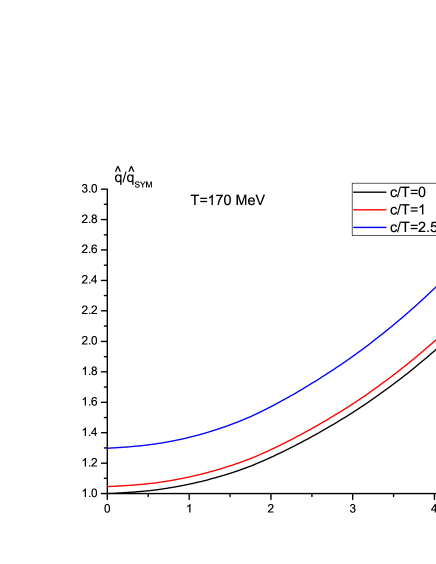
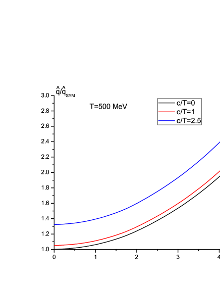
Figure 1: $\hat{q}/\hat{q}_{SYM}$ versus $\mu/T$ with fixed $c/T$. Left: $T=170MeV$. Right: $T=500MeV$. In both panels from top to bottom, $c/T=2.5,1,0$, respectively.

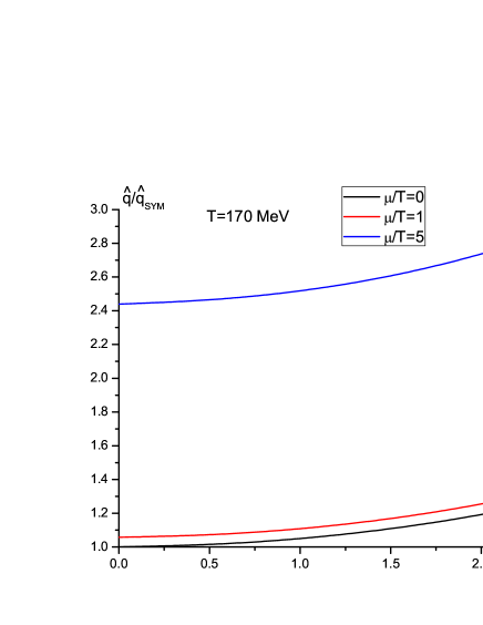
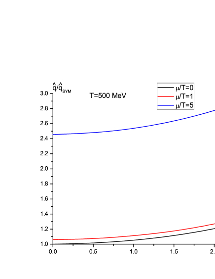
Figure 2: $\hat{q}/\hat{q}_{SYM}$ versus $c/T$ with fixed $\mu/T$. Left: $T=170MeV$. Right: $T=500MeV$. In both panels from top to bottom, $\mu/T=5,1,0$, respectively.

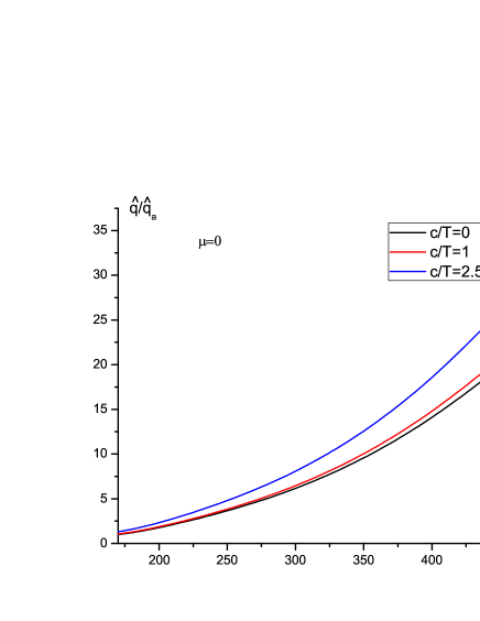
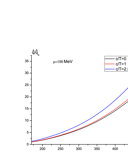
Figure 3: $\hat{q}/\hat{q}_{a}$ versus $T$ with fixed $c/T$. Left: $\mu=0$. Right: $\mu=100MeV$. In both panels from top to bottom, $c/T=2.5,1,0$, respectively.

Let’s discuss results. First, we analyze how $\mu$ and $c$ modify $\hat{q}$. For this purpose, we plot $\hat{q}/\hat{q}_{SYM}$ as a function of $\mu/T$ with fixed $c/T$ for two different temperatures in Fig.1, where the left panel is for $T=170MeV$ while the right $T=500MeV$. From both panels, one sees at fixed $c/T$, increasing $\mu/T$ leads to increasing $\hat{q}/\hat{q}_{SYM}$, indicating the inclusion of chemical potential increases the jet quenching parameter, in accord with that found in FL ; SD . Likewise, one can see from Fig.2 that at fixed $\mu/T$, $\hat{q}/\hat{q}_{SYM}$ increases as $c/T$ increases, implying the inclusion of nonconformality increases the jet quenching parameter, similar to AS . Thus, one concludes that the inclusion of chemical potential and nonconformality both increase the jet quenching parameter thus enhancing the energy loss, consistently with the findings of the drag force YH .

Also, we want to understand the $T$ dependence of $\hat{q}$ for this model. To this end, we plot $\hat{q}/\hat{q}_{a}$, with $\hat{q}_{a}|_{c=\mu=0,T=170MeV}$, versus $T$ in Fig.3, where the left panel is for $\mu=0$ while the right $\mu=100MeV$. From these figures, one finds with fixed $c/T$, $\hat{q}/\hat{q}_{a}$ increases as $T$ increases, as expected.

Finally, we would like to make a comparison to implications of experiment data. In Tab. 1, we present some typical values of $\hat{q}$, where we have taken $N_{c}=3$ and $\alpha_{SYM}=0.5$ (reasonable for temperatures not far above QCD phase transition), and $\lambda=6\pi$ liu . One finds that most of the values are consistent with the extracted values from RHIC data ($5\sim 25GeV^{2}/fm$) KFE ; JD . On the other hand, since the presence of $\mu$ and $c$ both enhance the jet quenching parameter, one may infer that increase $\mu$ and $c$ may lower the possible allowed domain of $T$ for the computed $\hat{q}$ to agree with the experiment data.

$T\setminus(\mu,c)$	(0, 0)	(0, 0.3)	(0, 0.7)	(0.1, 0)	(0.1, 0.3)	(0.1, 0.7)	(0.3, 0)	(0.3, 0.3)	(0.3, 0.7)
$0.3$	4.50	4.71	5.70	4.53	4.74	5.73	4.76	4.98	6.0
$0.4$	10.61	10.89	12.19	10.64	10.93	12.23	10.94	11.23	12.56
$0.5$	20.69	21.02	22.65	20.70	21.06	22.70	21.08	21.45	23.10

Table 1: Typical values of $\hat{q}$ in $GeV^{2}/fm$, where the first line denotes $(\mu,c)$ and the first column indicates $T$. Here $T,\mu,c$ are all expressed in units of $GeV$.

IV Conclusion

In this paper, we studied the jet quenching parameter in a soft wall model with finite temperature and chemical potential. The dual space geometry is AdS-RN black hole (describe finite temperature and density in the boundary theory) multiplied by a background warp factor (generate confinement). Our motivation rests on the earlier studies of the free energy PCO , imaginary potential zq and drag force YH in such a model. It turns out that the inclusion of chemical potential and nonconformality both increase the jet quenching parameter thus enhancing the energy loss, in agreement with the findings of the drag force YH . Also, we attempted to make a comparison to implications of experiment data and found the theoretical estimates agree well with experiment results. Finally, our results suggested that increase $\mu$ and $c$ may lower the possible allowed domain of $T$ for the computed $\hat{q}$ to agree with the experiment data.

Admittedly, the SW_T,μ model has some drawbacks. The primary disadvantage is that it is not a consistent model since it doesn’t solve the Einstein equations. Studying the jet quenching parameter in some consistent models, e.g. SH ; SH1 ; DL0 ; RCR would be informative (but note that the metrics of those models are only known numerically, so the calculations are very complex). Moreover, the SW_T,μ model may miss a part about the phase transition DL1 ; RG2 ; FZ and the effect of non-trivial dilaton field UG1 ; JNO ; MM ). Considering these effects would also be instructive. These will be left for further studies.

V Acknowledgments

This work is supported by the NSFC under Grants Nos. 11705166, 11947410, and Zhejiang Provincial Natural Science Foundation of China No. LY19A050001 and No. LY18A050002.

References

- (1) E. V. Shuryak, Nucl. Phys. A, 750: 64 (2005)
- (2) K. Adcox et al [PHENIX Collaboration], Nucl. Phys. A, 757: 184 (2005)
- (3) J. Adams et al [STAR Collaboration], Nucl. Phys. A, 757: 102 (2005).
- (4) X. N. Wang and M. Gyulassy, Phys. Rev. Lett., 68: 1480 (1992)
- (5) R. Baier, Y. L. Dokshitzer, A. H. Mueller, S. Peigne, and D. Schiff, Nucl. Phys. B, 484: 265 (1997)
- (6) X. N. Wang, arXiv:1906.11998
- (7) S. Cao and X. N. Wang, arXiv:2002.04028
- (8) J. M. Maldacena, Adv. Theor. Math. Phys., 2: 231 (1998)
- (9) O. Aharony, S. S. Gubser, J. Maldacena, H. Ooguri, and Y. Oz, Phys. Rept., 323: 183 (2000)
- (10) S. S. Gubser, I. R. Klebanov, and A. M. Polyakov, Phys. Lett. B, 428: 105 (1998)
- (11) J. Casalderrey-Solana, H. Liu, D. Mateos, K. Rajagopal, and U. A. Wiedemann, arXiv:1101.0618
- (12) A. Adams, L. D. Carr, T. Schfer, P. Steinberg, and J. E. Thomas, New J. Phys., 14: 115009 (2012)
- (13) H. Liu, K. Rajagopal, and U. A. Wiedemann, Phys. Rev. Lett., 97: 182301 (2006)
- (14) H. Liu, K. Rajagopal and U. A. Wiedemann, JHEP, 0703: 066 (2007)
- (15) N. Armesto, J. D. Edelstein, and J. Mas, JHEP, 0609: 039 (2006)
- (16) Z. q. Zhang, D. f. Hou, and H. c. Ren, JHEP, 1301: 032 (2013)
- (17) B. Pourhassan and J. Sadeghi, Can. J. Phys., 91: 995 (2013)
- (18) K. Bitaghsir Fadafan, Eur. Phys. J. C, 68: 505 (2010)
- (19) F. l. Lin and T. Matsuo, Phys. Lett. B, 641: 45-49 (2006)
- (20) S. D. Avramis and K. Sfetsos, JHEP, 0701: 065 (2007)
- (21) J. Sadeghi and B. Pourhassan, Int. J. Theor. Phys., 50: 2305 (2011)
- (22) K. Bitaghsir Fadafan, B. Pourhassan, and J. Sadeghi, Eur. Phys. J. C, 71: 1785 (2011)
- (23) Z. q. Zhang and K, Ma, Eur. Phys. J. C, 78: 532 (2018)
- (24) D. n. Li, J. f. Liao, and M. Huang, Phys. Rev. D, 89: 126006 (2014)
- (25) U. Gursoy, E. Kiritsis, G. Michalogiorgakis, and F. Nitti, JHEP, 0912: 056 (2009)
- (26) R. Rougemont, A. Ficnar, S. Finazzo, and J. Noronha, JHEP, 1604: 102 (2016)
- (27) M. Chernicoff, D. Fernandez, D. Mateos, and D. Trancanelli, JHEP, 1208: 041 (2012)
- (28) D. Giataganas, JHEP, 1207: 031 (2012)
- (29) S. Li, K. A. Mamo, and H. U. Yee, Phys. Rev. D, 94: 085016 (2016)
- (30) A. Ficnar, S. S. Gubser, and M. Gyulassy, Phys. Lett. B, 738: 464 (2014)
- (31) A. Buchel, Phys. Rev. D, 74: 046006 (2006)
- (32) M. Benzke, N. Brambilla, M. A. Escobedo, and A. Vairo, JHEP, 1302: 129 (2013)
- (33) E. Caceres and A. Guijosa, JHEP, 0612: 068 (2006)
- (34) S. y. Li, K. A. Mamo, and H. U. Yee, Phys. Rev. D, 94: 085016 (2016)
- (35) E. Nakano, S. Teraguchi, and W. Y. Wen, Phys.Rev. D, 75: 085016 (2007)
- (36) A. Saha and S. Gangopadhyay, Phys. Rev. D, 101: 086022 (2020).
- (37) A. Karch, E. Katz, D. T. Son, and M. A. Stephanov, Phys. Rev. D, 74: 015005 (2006)
- (38) P. Colangelo, F. Giannuzzi, and S. Nicotri, Phys. Rev. D, 83: 035015 (2011)
- (39) Z. q. Zhang and X. Zhu, Phys. Lett. B, 793: 200 (2019)
- (40) Y. Xiong, X. Tang, and Z. Luo, Chin. Phys. C 43: 113103 (2019)
- (41) O. Andreev, Phys. Rev. D, 81: 087901 (2010)
- (42) C. Park, D. Y. Gwak, B. H. Lee, Y. Ko, and S. Shin, Phys. Rev. D, 84: 046007 (2011)
- (43) P. Colangelo, F. Giannuzzi, and S. Nicotri, JHEP, 05: 076 (2012)
- (44) C. Ewerz, T. Gasenzer, M. Karl, and A. Samberg, JHEP, 05: 070 (2015)
- (45) X. Chen, S. Q. Feng, Y. F. Shi, and Y. Zhong, Phys. Rev. D, 97: 066015 (2018)
- (46) H. Liu, K. Rajagopal, and Y. Shi, JHEP, 08: 048 (2008)
- (47) K.F. Eskola, H. Honkanen, C.A. Salgado, U.A. Wiedemann.: Nucl. Phys. A 747, 511 (2005).
- (48) J. D. Edelstein and C. A. Salgado, AIP Conf.Proc., 1031: 207 (2008)
- (49) S. He, M. Huang and Q. S. Yan, JHEP, Phys. Rev. D, 83: 045034 (2011)
- (50) S. He, S. Y. Wu, Y. Yang, and P. H. Yuan, JHEP, 1304: 093 (2013)
- (51) D. n. Li and M. Huang, JHEP, 1311: 088 (2013)
- (52) R. Critelli, J. Noronha, J. N. Hostler, I. Portillo, C. Ratti and R. Rougemont, Phys. Rev. D, 96: 096026 (2017)
- (53) D. n. Li, S. He, M. Huang, and Q. S. Yan, JHEP, 1109: 041 (2011)
- (54) R. G. Cai, S. He, and D. n. Li, JHEP, 1203: 033 (2012)
- (55) F. Zuo and Y. H. Gao, JHEP, 1407: 147 (2014)
- (56) U. Gursoy, E. Kiritsis, and F. Nitti, JHEP, 0802: 019 (2008)
- (57) M. Mia, K. Dasgupta, C. Gale, and S. Jeon, Phys. Rev. D, 82: 026004 (2010)
- (58) J. Noronha. Phys. Rev. D, 81: 045011 (2010)