Radiative cooling rates, ion fractions, molecule abundances and line emissivities including self-shielding and both local and metagalactic radiation fields

Abstrakt

We use the spectral synthesis code cloudy to tabulate the properties of gas for an extensive range in redshift ($z=0$ - $9$), temperature ($\log T[K]=1$ - $9.5$), metallicity ($\log Z/\mathrm{Z}_{\odot}=-4$ - $+0.5$, $Z=0$), and density ($\log n_{\mathrm{H}}[\,\mathrm{cm}^{-3}]=-8$ - $+6$). This therefore includes gas with properties characteristic of the interstellar, circumgalactic and intergalactic media. The gas is exposed to a redshift-dependent UV/X-ray background, while for the self-shielded lower-temperature gas (i.e. ISM gas) an interstellar radiation field and cosmic rays are added. The radiation field is attenuated by a density- and temperature-dependent column of gas and dust. Motivated by the observed star formation law, this gas column density also determines the intensity of the interstellar radiation field and the cosmic ray density. The ionization balance, molecule fractions, cooling rates, line emissivities, and equilibrium temperatures are calculated self-consistently. We include dust, cosmic rays, and the interstellar radiation field step-by-step to study their relative impact. These publicly available tables are ideal for hydrodynamical simulations. They can be used stand alone or coupled to a non-equilibrium network for a subset of elements. The release includes a C routine to read in and interpolate the tables, as well as an easy to use python graphical user interface to explore the tables.

1 Introduction

Radiative processes are a critical ingredient for all models that include baryons. Radiative losses are not only crucial for the formation of stars and therefore for the ignition of the cosmic baryon cycle, they are also heavily used in observational astronomy to classify the properties of gas within galaxies (interstellar medium, ISM), around galaxies (circumgalactic medium, CGM) and in between galaxies (intergalactic medium, IGM). The photons that are emitted at specific energies are important tracers for the composition, physical properties (e.g. density, temperature), and the movement of the gas (e.g. turbulence, inflow, outflows).

Determining the radiative cooling rate of a parcel of gas relies on a series of intertwined chemical reactions of species that can also interact with the ambient radiation field. A full implementation of these processes in a simulation would therefore require solving a large chemical network together with a coupled radiative transfer code for each resolution element at each timestep. While this can currently be done for a limited set of species in small-scale simulations of galaxy formation and evolution (e.g. isolated galaxies, or patches of the ISM), it is computationally too expensive to do in a large cosmological volume. A popular compromise to include radiative processes in simulations is to tabulate the cooling (and heating) rates. Therefore, the way these tabulated rates are calculated can be arbitrarily complicated without affecting the runtime of the simulation.

Traditionally, radiative cooling functions were calculated under the assumption of an optically thin gas in collisional ionization equilibrium (CIE, e.g. Cox & Tucker 1969; Dalgarno & McCray 1972; Raymond et al. 1976; Shull & van Steenberg 1982; Gaetz & Salpeter 1983; Boehringer & Hensler 1989; Sutherland & Dopita 1993). The ionization rates in CIE (and therefore the recombination rates and the radiative losses, $\Lambda$) are proportional to the number of collisions between particles (electrons and atoms). As hydrogen is the most abundant element in the Universe, the number density of particles scales with the hydrogen number density $n_{\mathrm{H}}$ and the normalised cooling rate $\Lambda/n_{\mathrm{H}}^{2}\,[\mathrm{erg}\,\mathrm{s}^{-1}\,\mathrm{cm}^{3}]$ is only a function of temperature (case I in Table 1). In this case, the contribution of individual elements scales linearly with their element abundance and the cooling rate for each chemical element can either be provided in terms of tables (e.g. Boehringer & Hensler 1989) or fitting functions (e.g. Dalgarno & McCray 1972).

When including photo-ionisation, the gas is over-ionised compared to the CIE case. This leads to different cooling rates caused by the different ion fractions of each individual element (e.g. Efstathiou, 1992; Wiersma et al., 2009). As the photo-ionization rate scales with the number of particles to ionise (again approximated by $n_{\mathrm{H}}$), while collisional processes scale with $n_{\mathrm{H}}^{2}$, the normalised cooling rate $\Lambda/n_{\mathrm{H}}^{2}\,[\mathrm{erg}\,\mathrm{s}^{-1}\,\mathrm{cm}^{3}]$ that combines both types of processes is a function of both density and temperature (case II in Table 1).

As the radiation field is not constant throughout the Universe, additional dependences are introduced. In galaxy-scale or cosmological simulations, a redshift-dependent uniform UV background (UVB) is often used as radiation field, which adds a redshift dependence to the tabulated cooling rates (case IIa in Table 1, e.g. Wiersma et al. 2009, hereafter: W09). W09 showed that at the peak of the cooling function, between temperatures of $10^{4}$ and $10^{6}\,\mathrm{K}$, the cooling rate is reduced by up to an order of magnitude compared to the CIE case when photoionization from the UVB is included.

Gnedin & Hollon (2012) tabulate the properties of photo-ionized gas for general radiation fields from stars or active galactic nuclei (AGN). They parametrize their incident spectrum with 4 independent values, one for the intensity and three that define its shape (case IIb in Table 1), resulting in an equal number of additional dimensions (7 in total, including density, temperature, and metallicity) for their tabulated cooling rates of optically thin gas in ionization equilibrium.

At temperatures between $10^{4}$ and $\approx 5\times 10^{6}\,\,\mathrm{K}$ the cooling timescale can become shorter than the recombination timescale, leading to a “recombination lag". This rapidly cooling gas is therefore over-ionized compared to ionization equilibrium (e.g. Kafatos, 1973). Gnat & Sternberg (2007) provide tables of radiative cooling rates including this non-equilibrium effect. Their calculations start with initially hot ($T>5\times 10^{6}\,\,\mathrm{K}$) gas that cools either at constant density or constant pressure in the absence of a radiation field. The resulting cooling functions are smoother with a less pronounced peak due to hydrogen recombination compared to the equilibrium rates. As metal line cooling is important, their tabulated cooling rates also depend on the gas metallicity (case N-I, Table 1).

Tabulka 1: In collisional ionization equilibrium (CIE), the cooling rate $\Lambda$ scales with the hydrogen number density, $n_{\mathrm{H}}^{2}$, and the term $\Lambda/n_{\mathrm{H}}^{2}$ therefore only depends on the temperature $T$. Including extra processes (rows) induces additional dependences on $n_{\mathrm{H}}$, redshift $z$, hydrogen column density $N_{\mathrm{H}}$, gas metallicity $Z$, as well as the intensity, $I$, and shape of the radiation field (RF).

Case		$\Lambda/n_{\mathrm{H}}^{2}$ dependence
Ionization equilibrium
I	CIE	$T$
II	Photo-ionization	$T,n_{\mathrm{H}}$
IIa	Photo-ionization (UVB)	$T,n_{\mathrm{H}},z$
IIb	Photo-ionization (general RF)	$T,n_{\mathrm{H}},Z,I,\mathrm{shape}$
III	UVB, self-shielded gas	$T,n_{\mathrm{H}},z,Z,N_{\mathrm{H}}$
IV	UVB, ISRF, self-shielded gas	$T,n_{\mathrm{H}},z,Z,N_{\mathrm{H}},I,\mathrm{shape}$
this work:
Va	UVB, unshielded gas	$T,n_{\mathrm{H}},z,Z$
Vb	UVB, self-shielded gas	$T,n_{\mathrm{H}},z,Z$
Vc	UVB, ISRF, unshielded gas	$T,n_{\mathrm{H}},z,Z$
Vd	UVB, ISRF, self-shielded gas	$T,n_{\mathrm{H}},z,Z$
Non-equilibrium
N-I	CIE	$T,Z$
N-IIa	Photo-ionization (UVB)	$T,n_{\mathrm{H}},z,Z$

Similar to the approach from Gnat & Sternberg (2007), Oppenheimer & Schaye (2013) use their non-equilibrium reaction network to provide tabulated cooling and photo-heating rates by following hot gas as it cools either at constant pressure or constant density. In contrast to Gnat & Sternberg (2007), Oppenheimer & Schaye (2013) include a redshift-dependent background radiation field and they tabulate their cooling rates for each ion of each considered element. As a hydrodynamic code typically does not trace the individual ion abundances, they also provide tabulated ion fractions of 11 elements, depending on the hydrogen number density, temperature, and metallicity of the gas, as well as the redshift for the background radiation field (case N-IIa in Table 1). Oppenheimer & Schaye (2013) conclude that non-equilibrium effects are reduced when the background radiation field is included.

All above approaches focus on ionized gas with temperatures above $10^{4}\,\,\mathrm{K}$, as is typical for the CGM and IGM. At these temperatures, molecules cannot form, dust grains are quickly destroyed by thermal sputtering (e.g. Tielens et al. 1994) and gas is optically thin to ionizing radiation. In the ISM, the incident radiation is however attenuated by gas and dust and can self-shield from photo-ionizing or photo-dissociating radiation. As the ion fractions depend on the photo-ionization rate, the cooling rate varies with the hydrogen column density $N_{\mathrm{H}}$ (case III in Table 1). This can lead to structures where the illuminated side of a gas parcel is ionized, but deeper into the cloud, the gas can remain neutral and cold.

In neutral gas, the formation of molecules and the existence of dust grains further complicates the picture. Dust grains and molecules shield different parts of the intrinsic radiation field and the reaction rates of various molecules have a non-trivial dependence on the shape of the spectrum. In addition, an important formation channel of $\mathrm{H}_{\mathrm{2}}$ depends on dust grains as catalysts, which results in a non-trivial relation between the gas metallicity and the $\mathrm{H}_{\mathrm{2}}$ abundance.

The ISM gas resolution elements in hydrodynamic simulations can have a large variety of thermal and chemical histories: from gas that cools through thermal instabilities and is accreted from the galaxy halo to dense gas that is heated by nearby stellar feedback events. Tabulating non-equilibrium cooling rates and other chemical properties in a similar way (i.e. cooling from high temperatures) is therefore not a good approach. Chemical networks that solve a large number of differential equations to follow the thermo-chemical evolution of the gas particles are required to include non-equilibrium effects in the ISM.

grackle (Smith et al., 2017) is an open-source chemistry and cooling library that allows users to include hydrogen and helium non-equilibrium chemistry directly in the simulation. The primordial network includes the self-shielding approximation from Rahmati et al. (2013) (hereafter, R13). The cooling and heating rates from metals are calculated with cloudy under the assumption of ionization equilibrium, and tabulated for the UV background from Haardt & Madau (2012). In the 2017 grackle release, the metal cooling and heating rates assume that the gas is optically thin to the UV background and solar abundances. Combining the primordial network with the tabulated metal rates leads to inconsistencies in their electron fractions if self-shielding is included. The free electron fraction from hydrogen and helium used in the primordial network that includes self-shielding can be much lower than the free electron fraction from hydrogen and helium used in the optically thin cloudy tables. The metal cooling rates are therefore based on gas that is too highly ionized, leading to too high cooling rates for self-shielded gas. This has been discussed in Hu et al. (2017) and Emerick et al. (2019) produced metal cooling tables for grackle that include self-shielding of the UV background by hydrogen and helium, while shielding on metals and dust grains is neglected. Furthermore, as dust grains are not included in the cloudy calculations, grackle’s shielding column lacks H₂. The rates are calculated using a shielding length based on the local Jeans length (limited to a physical size of 100 pc) and for a single metallicity with solar relative abundances.

Glover et al. (2010) present an ISM model for CO formation in turbulent molecular clouds within the ISM, including, in addition to hydrogen and helium, both carbon and oxygen chemistry. Reduced chemical networks have also been used to study the dependence of the abundance of molecules, such as $\mathrm{H}_{\mathrm{2}}$ and CO, on the cosmic ray rate (Bisbas et al., 2015; Bisbas et al., 2017) or (in addition) on metallicity and the radiation field intensity (e.g. Bialy & Sternberg, 2015; Bisbas et al., 2019). An extended chemical network with 272 chemical reactions that follow the evolution of 157 species (among these: 20 different molecules) is described in Richings et al. (2014a) for optically thin gas, and Richings et al. (2014b) for shielded gas. The effects of self-shielding compared to the assumption of optically thin gas, as well as the impact of the radiation field strength and gas metallicity on molecule abundances, are demonstrated in simulations of isolated galaxies by Richings & Schaye (2016). These large chemical networks that also calculate metals in non-equilibrium are computationally expensive, as the number of reactions increases rapidly with every included species.

The aim of this work is to provide tables of gas properties in ionization equilibrium that include radiation by a UV background and, optionally, from an interstellar radiation field (ISRF) for both unshielded (or optically thin to the radiation field) and self-shielded gas. The large number of dimensions would make the tables expensive to produce and would also lead to large memory requirements during any simulation run using the tables. More importantly, neither the shielding gas column density nor the local radiation field is generally known on the fly in large-scale simulations.

We solve this issue by assuming that the gas is self-gravitating and hence that its coherence scale is the local Jeans length (Schaye, 2001a, b). Note that Rahmati et al. (2013) showed that this assumption reproduces the shielding lengths in their cosmological, radiative transfer simulations. By setting the shielding column density to half of the local Jeans column density we remove the $N_{\mathrm{H}}$ dimension. In addition, we assume that the incident radiation field, which could be described by an arbitrary number of parameters, comes in two flavours: (1) the redshift-dependent model of the UVB by Faucher-Giguère (2020) (hereafter: FG20), modified to make the treatment of attenuation before H i and He ii reionization more self-consistent, and (2) optionally, a local interstellar radiation field (ISRF) with a constant spectral shape and a normalization that depends on the local Jeans column density of the gas as suggested by the observed Kennicutt-Schmidt (Kennicutt, 1998) star formation law (case Vc,d in Table 1). For comparison, we also include the unshielded versions of the same tables (case Va,c in Table 1). We use the spectral synthesis code cloudy v17.01, last described in Ferland et al. (2017), to transmit the spectrum through the gas (for self-shielded gas), calculate the equilibrium ionization states of all atomic ions, and follow the formation and destruction of molecules to obtain the resulting cooling and heating rates for all included processes.

While we do not take non-equilibrium effects into account, the tables can easily be coupled to non-equilibrium networks that calculate the abundances of H and He, an approach that captures non-equilibrium effects on metals caused by the non-equilibrium free electron density (see Appendix A.2).

The data products include a set of tables in hdf5 format of cooling and heating rates (also per element), ion and molecule fractions, and line emissivities, a routine that reads in and interpolates the cooling rates (written in C), as well as a python-based graphical user interface (gui) to visualise the table content. In equations that refer directly to individual hdf5 datasets, a line with the dataset name is added (e.g. dataset: ShieldingColumnDensityRef in Eq. 6). Figures that can be reproduced directly with the provided gui are labelled accordingly in the figure captions. The python and C routines and additional information on how to download the tables as well as examples can be found on dedicated web pages (http://radcool.strw.leidenuniv.nl/ or https://www.sylviaploeckinger.com/radcool).

The methods are described in detail in Sec. 2, including how the shielding column (Sec. 2.1), the radiation field (Sec. 2.2), and the dust content (Sec. 2.4) vary within the four-dimensional grid in redshift, temperature, metallicity, and density. We present the data products in Sec. 4, where the individual tables of the full set are presented and their information content is listed and explained. In Sec. 5 we highlight a few key results, such as the dependence of the thermal equilibrium temperatures and the most important phase transitions (ionized - neutral, neutral - molecular) on redshift, metallicity, and the radiation field. We summarise the findings in Sec. 7 and add sections on how to use (Appendix A) and reproduce (Appendix C) the provided tables.

The grid spacing in temperature, density, redshift, and metallicity as well as most of the tabulated properties are in $\log$. Throughout the paper $\log$ refers to $\log_{\mathrm{10}}$ and we use $10^{-50}$ as a floor value for properties that would be zero. All bins are generally equally spaced in $\log$ but the metallicity dimension has an additional bin: primordial abundances ($Z=0$, referred to as $\log Z/\mathrm{Z}_{\odot}=-50$).

2 Method

For the calculation of cooling and heating rates as well as ionization stages and molecular fractions, we use version 17.01 of the photoionization code cloudy (Ferland et al., 1998; Ferland et al., 2017). cloudy is a powerful and widely used open source code that can calculate the ionization, chemical, and thermal equilibrium state of gas exposed to an external radiation field.

Our basic setup is a large grid of cloudy runs with dimensions $z$ (redshift), $T$ (temperature [K]), $Z$ (metallicity [${\mathrm{Z}}_{\odot}$]), and $n_{\mathrm{H}}$ (total hydrogen number density [$\,\mathrm{cm}^{-3}$]). The aim of this work is to provide tables that cover the full range of gas properties typically occurring in galaxy-scale or cosmological simulations (see Table 2). Throughout the paper we use the solar metallicity (${\mathrm{Z}}_{\odot}=0.0134$) and solar abundance ratios from Asplund et al. (2009) (see Table 3).

Tabulka 2: All gas properties are tabulated on an equally spaced grid in the dimensions: redshift $z$, gas temperature $\log T$, metallicity $\log Z/{\mathrm{Z}}_{\odot}$, and gas density $\log n_{\mathrm{H}}$. The grid points for each dimension range from their minimum (column 3) to their maximum (column 4) value, with the spacing $\Delta$ between the grid points listed in column 5. For metallicity an additional field is included for primordial abundances ($\log Z/{\mathrm{Z}}_{\odot}=-50$, i.e. $Z=0$). The resulting number of bins per dimension in column 6 leads to a total of 3,089,636 grid points for each table.

	unit	min	max	$\Delta$	extra	nbins
z		0	9	0.2		46
$\log T$	$[\,\mathrm{K}]$	1	9.5	0.1		86
$\log Z/{\mathrm{Z}}_{\odot}$		-4	0.5	0.5	-50 ($Z=0$)	11
$\log n_{\mathrm{H}}$	$[\,\mathrm{cm}^{-3}]$	-8	6	0.2		71

For every grid point in the tables that include self-shielding, the chosen incident radiation field is set to propagate through a slab of plane-parallel gas with the given properties ($T$, $Z/{\mathrm{Z}}_{\odot}$, $n_{\mathrm{H}}$) until its shielding column density $N_{\mathrm{sh}}$ is reached. cloudy bins the gas column into individual zones of adaptive widths and in each zone the chemical properties and ionization states are calculated and the resulting output spectrum is passed as input into the next zone. Within each gas column, the total hydrogen number density as well as the gas temperature are set to remain constant, while the ion fractions, electron densities, and molecule fractions depend on the depth into the slab of gas. For unshielded gas, the properties of the first zone are tabulated (1-zone model), while for self-shielded gas the same properties are tabulated for the last zone, where $N_{\mathrm{H}}=N_{\mathrm{sh}}$.

For ionized gas in ionization equilibrium, the contribution of individual elements to the total cooling and heating rates can be calculated by running the same 1-zone cloudy models once with the full abundance set and once excluding individual elements. The difference in the rates can then be attributed to the excluded element (this is done e.g. in W09). Here, this approach is not suitable, as a combination of elements is involved in the formation of molecules and the shielding contributions from one species can affect the abundance of another species. We therefore run cloudy for each grid point only once and output the values for each cooling and heating channel, as listed in Tables 9 and 10. For a full list of gas properties tabulated for each grid point, see Sec. 4.

Tabulka 3: Solar abundances from Asplund et al. (2009) for individually tabulated elements with a total metallicity of Z = 0.0134.

Element	$n_{i}/n_{\mathrm{H}}$
H	1
He	$8.51\times 10^{-2}$
C	$2.69\times 10^{-4}$
N	$6.76\times 10^{-5}$
O	$4.90\times 10^{-4}$
Ne	$8.51\times 10^{-5}$
Mg	$3.98\times 10^{-5}$
Si	$3.24\times 10^{-5}$
S	$1.32\times 10^{-5}$
Ca	$2.19\times 10^{-6}$
Fe	$3.16\times 10^{-5}$

2.1 Column density

Tabulka 4: Overview of the Milky Way / solar neighbourhood values used to scale the interstellar radiation field, the CR rate and the D/G ratio.

				Description
$\log N_{\mathrm{H,0}}$	20.56		$\,\mathrm{cm}^{-2}$	Total hydrogen gas column density
$\log N_{\mathrm{sh,0}}$	20.26		$\,\mathrm{cm}^{-2}$	Total hydrogen shielding column density
$\Sigma_{\mathrm{g,0}}$	3.85		${\mathrm{M}}_{\odot}\,\mathrm{pc}^{-2}$	Total gas surface density
$(\mathrm{D/G})_{0}$	$5.623\times 10^{-3}$			Total dust mass to gas mass ratio for $Z={\mathrm{Z}}_{\odot}$
$\Sigma_{\mathrm{SFR,0}}$	$10^{-3}$		${\mathrm{M}}_{\odot}\,\mathrm{yr}^{-1}\mathrm{kpc}^{-2}$	SFR surface density
$J_{\mathrm{0}}$	$1.4\times 10^{-3}$		$\mathrm{erg}\,\mathrm{cm}^{-2}\,\mathrm{s}^{-1}$	Radiation field from stars ($4\pi\nu J_{\nu}$), defined at 1000 Å
$\Gamma_{\mathrm{Phot,0}}(\text{H\,{i}})$	$3.75\times 10^{-11}$		$\mathrm{s}^{-1}$	H i ionization rate
$\Gamma_{\mathrm{Phot,0}}(\text{He\,{i}})$	$3.10\times 10^{-12}$		$\mathrm{s}^{-1}$	He i ionization rate
$\Gamma_{\mathrm{Phot,0}}(\text{He\,{ii}})$	$1.43\times 10^{-14}$		$\mathrm{s}^{-1}$	He ii ionization rate
$\log\zeta_{0}$	$-15.7$		$\mathrm{s}^{-1}$	Cosmic ray hydrogen ionization rate

We have already established that the gas properties of self-shielded gas depend on the depth (i.e. gas column density) into the irradiated slab of gas. While algorithms to calculate the optical depths for each resolution element in a simulation have been developed (e.g Wünsch et al., 2018 for the grid code FLASH, Fryxell et al., 2000), the shielding column or optical depth can be expensive to calculate and is not generally known on the fly.

The shielding length is often approximated based on the gradient in the gas density $\rho$

$$L_{\mathrm{Sob}}=\frac{\rho}{|2\nabla\rho|}\,,$$ (1)

referred to as Sobolov approximation (used e.g. in Richings & Schaye, 2016; Hopkins et al., 2018), or is assumed to be close to the local Jeans length for self-gravitating gas (e.g. in Schaye, 2001b)

$$L_{\mathrm{J}}=\left(\frac{\gamma Xk_{\mathrm{B}}}{m^{2}_{\mathrm{H}}\mu G}\right)^{0.5}\left(\frac{T}{n_{\mathrm{H}}}\right)^{0.5}\,,$$ (2)

where $\gamma$ is the ratio of specific heats, $X$ is the hydrogen mass fraction, $k_{\mathrm{B}}$ is the Boltzmann constant, $m_{\mathrm{H}}$ is the proton mass, $\mu m_{\mathrm{H}}$ is the mean particle mass, $G$ is the gravitational constant and $n_{\mathrm{H}}$ and $T$ are the total hydrogen density and temperature. The resulting Jeans column density is

$$N_{\mathrm{J}} =\left(\frac{\gamma Xk_{\mathrm{B}}}{m^{2}_{\mathrm{H}}\mu G}\right)^{0.5}\left(n_{\mathrm{H}}T\right)^{0.5}\,.$$ (3)

The cloudy calculation stops when a specified total hydrogen column density is reached. Using the values for $\gamma$ and $\mu$ from the current cloudy zone leads to discontinuities in the shielding column densities at phase transitions as $\mu$ changes steeply (ionized - neutral: $\mu\approx 0.5\rightarrow 1$, atomic - molecular: $\mu\approx 1\rightarrow 2$). In addition, the last zone would preferentially be at the phase transition, as the shielding length suddenly decreases ($N_{\mathrm{J}}\propto\mu^{-0.5}$). We therefore use the values of primordial neutral gas (from Planck Collaboration et al., 2016) for the shielding column density: $X=0.7563$, $\gamma=5/3$, and $\mu=1.2328$, which results in

$$L_{\mathrm{J}}=0.9\,\mathrm{kpc}\,\left(\frac{T}{10^{4}\,\mathrm{K}}\right)^{\mathrm{0.5}}\left(\frac{n_{\mathrm{H}}}{1\,\mathrm{cm}^{-3}}\right)^{\mathrm{-0.5}}\,$$ (4)

and

$$\log N_{\mathrm{J}}\,[\,\mathrm{cm}^{-2}]=19.44+0.5\times(\log n_{\mathrm{H}}[\,\mathrm{cm}^{-3}]+\log T[K])\,.$$ (5)

The Jeans column density is defined in Schaye (2001a, b), and R13 showed that this approximation for the shielding column reproduces the results of full radiative transfer calculations for H i in cosmological simulations that however did not include a cold ISM. We use the Jeans length approximation here, as it has the additional advantage that $N_{\mathrm{J}}$ depends only on gas temperature and density, so no extra dimension $\nabla\rho$ is required in the tables.

We cover a large range of gas densities and temperatures (see Table 2) and the Jeans column density cannot be directly applied everywhere. High temperature gas ($T\gtrsim 10^{5}\,\,\mathrm{K}$) is mostly ionized and therefore optically thin, but as $N_{\mathrm{J}}\propto T^{0.5}$, its theoretical shielding length would continue to increase for a constant density. This leads to practical problems in cloudy, as the 1D shielding column starts to radiate thermal emission for high temperatures which results in an increasing radiation field with shielding column density. In addition, the shielding length can become very large for very low densities ($n_{\mathrm{H}}<10^{-6}\,\,\mathrm{cm}^{-3}$), leading to unrealistic coherence length scales corresponding to dynamical and sound crossing times that exceed the Hubble time. We therefore limit the length scale to $l_{\mathrm{max}}=100\,\mathrm{kpc}$, the total hydrogen column densities to $N_{\mathrm{max}}=10^{24}\,\,\mathrm{cm}^{-2}$ and use an asymptotic function for a smooth transition between low ($\lesssim 10^{3}\,\,\mathrm{K}$, shielded) and high ($\gtrsim 10^{5}\,\,\mathrm{K}$, optically thin) temperature gas.

The reference column density, $N_{\mathrm{ref}}$, is defined as

$$\log N_{\mathrm{ref}}= \log N^{\prime}_{\mathrm{ref}}-\frac{\log N^{\prime}_{\mathrm{ref}}-\log N_{\mathrm{min}}}{1+\left(\sqrt{T_{\mathrm{min}}T_{\mathrm{max}}}/T\right)^{k}}\,,$$ (6)

$$\mathrm{dataset:}\,\texttt{ShieldingColumnRef}$$

where $k=5/\ln(10)=2.17$ regulates the steepness of the transition between the asymptotes $N^{\prime}_{\mathrm{ref}}$ reached at $T\ll\sqrt{T_{\mathrm{min}}T_{\mathrm{max}}}$ and $N_{\mathrm{min}}$ at $T\gg\sqrt{T_{\mathrm{min}}T_{\mathrm{max}}}$. We will use $T_{\mathrm{min}}=10^{3}\,\,\mathrm{K}$ and $T_{\mathrm{max}}=10^{5}\,\,\mathrm{K}$. $N^{\prime}_{\mathrm{ref}}$ is based on the length and column density limited Jeans column density $N_{\mathrm{J}}$:

$$\log N^{\prime}_{\mathrm{ref}}\,[\,\mathrm{cm}^{-2}]=\mathrm{min}\begin{cases}\log N_{\mathrm{J}}&\\ \log l_{\mathrm{max}}\,n_{\mathrm{H}}\quad.&\\ \log N_{\mathrm{max}}&\end{cases}$$ (7)

$N_{\mathrm{min}}=l_{\mathrm{max}}\,n_{\mathrm{H,min}}=3.08\times 10^{15}\,\mathrm{cm}^{-2}$ is the column density used for the minimum density in the tables $n_{\mathrm{H,min}}=10^{-8}\,\,\mathrm{cm}^{-2}$.

Eqs. 6 and 7 are illustrated in Fig. 1. $N^{\prime}_{\mathrm{ref}}$ (dashed line) follows the Jeans length $N_{\mathrm{J}}$ (dotted lines) for low temperatures but is limited by $l>l_{\mathrm{max}}=100\,\mathrm{kpc}$ (grey area) at low densities and by $N_{\mathrm{max}}$ at high densities. Adding the asymptotic transition to $N_{\mathrm{min}}$ for $T\gg\sqrt{T_{\mathrm{min}}T_{\mathrm{max}}}$ leads to the final $N_{\mathrm{ref}}$ (solid lines). A plot of $\log N_{\mathrm{ref}}$ as a function of density and temperature is presented in Fig. 2.

For unshielded tables, the cloudy calculation is stopped for each grid point after the first zone, where the maximum size of the first zone is set to $\Delta r=10^{20}\,\mathrm{cm}$. The code stops adding zones when the total hydrogen column density exceeds the shielding column density

$$\log N_{\mathrm{sh}}= \begin{cases}\log(0.5\times N_{\mathrm{ref}})&\mathrm{for\,shielded\,gas}\\ \log(\Delta r\times n_{\mathrm{H}})&\mathrm{for\,optically\,thin\,gas}\end{cases}$$ (8)

$$\mathrm{dataset:}\,\texttt{ShieldingColumn}$$

$N_{\mathrm{sh}}$ is therefore the column density from the edge of the self-gravitating gas clump/disc to its centre/midplane, while $N_{\mathrm{ref}}$ describes the total column column density through the gas clump. The shielding column density to the last zone of the cloudy column is tabulated as dataset ShieldingColumn. Depending on the thickness of the last zone, a small deviation from $0.5N_{\mathrm{ref}}$ is possible. For unshielded runs, ShieldingColumn is the column density of the first zone, while the values for $N_{\mathrm{ref}}$ in dataset ShieldingColumnRef are the same for both unshielded and self-shielded runs.

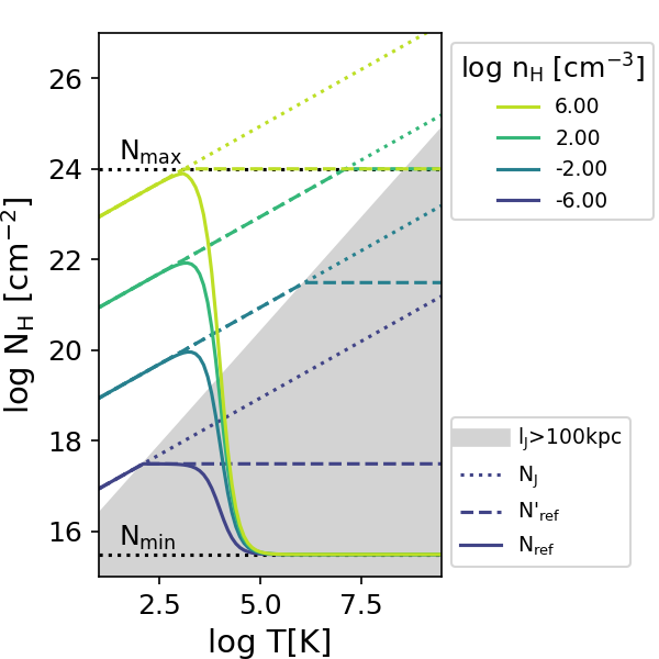
Obrázek 1: Temperature dependence of the discussed hydrogen column densities for selected gas densities $n_{\mathrm{H}}$ (different colors). The Jeans column density $N_{\mathrm{J}}$ (Eq. 5, dotted lines) increases with temperature as $N_{\mathrm{J}}\propto T^{0.5}$ for a constant gas density. $N^{\prime}_{\mathrm{ref}}$ (Eq. 7, dashed lines) follows the Jeans column density for low temperatures but is limited by a maximum column density $N_{\mathrm{max}}=10^{24}\,\mathrm{cm}^{-2}$ and a maximum length scale of $l_{\mathrm{max}}=100\,\mathrm{kpc}$ (the grey area indicates where $l_{\mathrm{J}}>100\,\mathrm{kpc}$). The final reference column density $N_{\mathrm{ref}}$ (Eq. 6, solid lines) includes the asymptotic transition in temperature from self-shielded gas to optically thin gas with a minimum column density $N_{\mathrm{min}}$. The values for $N_{\mathrm{ref}}$, which corresponds to twice the shielding column density, over the full temperature-density parameter space are shown in Fig. 2.

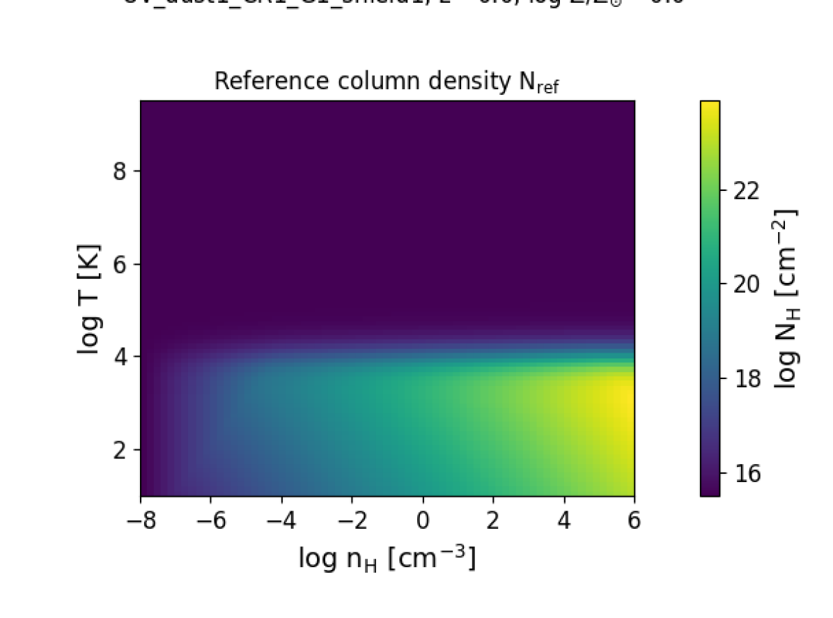
Obrázek 2: Reference column density $N_{\mathrm{ref}}$ (Eq. 6) for hydrogen number density $n_{\mathrm{H}}$ and gas temperature $T$. $N_{\mathrm{ref}}$ corresponds to twice the shielding column density. Figure made with provided gui.

2.2 Radiation field

The incident spectrum in all tables includes a redshift dependent UVB based on FG20 (Sec. 2.2.1), as well as the cosmic microwave background (CMB) as a blackbody spectrum with a redshift dependent temperature of $T_{\mathrm{CMB}}=T_{0}\,(1+z)$ with $T_{0}=2.725\,\mathrm{K}$. In some tables a local radiation field is added that models the contribution from nearby stars (Sec. 2.2.2) in the ISM.

2.2.1 UV background radiation field

The spectrum for the UVB from distant galaxies and active galactic nuclei (AGN) is based on FG20, which consists of three main contributions. First, the radiation field from stars (for $z\leq 8$) is from the BPASS (Eldridge et al., 2017; Stanway & Eldridge, 2018) spectrum for a stellar population with a constant star formation rate at an age of 300 Myr and a metallicity of $0.1\mathrm{Z}_{\odot}$. This spectrum is dust attenuated with a constant $E(B-V)=0.129$. The redshift-dependent normalization is chosen to match the observed total UV emissivity from GALEX for $z<2$ (Chiang et al., 2019) and the rest-frame UV galaxy luminosity function from Bouwens et al. (in prep.) for $z>2$ at 8.3 eV (1500Å). Second, the radiation from AGN is modelled by combining spectral templates of obscured (75 per cent) and unobscured AGN (25 per cent) and the spectrum is normalized to the AGN ionizing emissivity from Shen et al. (2020) at 912Å. Third, recombination emission from the photons absorbed by the ISM of star-forming galaxies as well as the recombination emission lines related to the “sawtooth" absorption by He ii Lyman series lines.

In addition to redshift-dependent spectra, FG20 also provide effective photo-ionization $\Gamma_{\mathrm{x,eff}}$ and photo-heating rates $\dot{q}_{\mathrm{x,eff}}$ (with $x=\left\{\right.$H i, He i, He ii $\left.\right\}$) that are constructed to produce a prescribed volume-averaged ionized fraction (H ii and He iii) for each redshift, assuming photoionization equilibrium. These effective rates are lower than the rates calculated directly from the spectra before reionization in order to match the electron scattering optical depth of $\tau_{\mathrm{e}}=0.054$, the best fit value to the Planck 2018 CMB data (Planck Collaboration et al., 2018). The best model in FG20 uses reionization redshifts of $z_{\mathrm{rei,HI}}=7.8$ and $z_{\mathrm{rei,HeII}}=3.5$, while at $z<z_{\mathrm{rei,HI}}-\Delta z_{\mathrm{rei,HI}}=7.2$ and $z<z_{\mathrm{rei,HeII}}-\Delta z_{\mathrm{rei,HeII}}=3$, reionization is completed and the respective effective rates match the rates from the spectra.

For the UVB used in this work, we modify the spectra from FG20 for $z>3$ so that they yield rates that match the effective photo-ionization and photo-heating rates before H i and He ii reionization. The details of this method as well as the resulting rates are shown in Appendix B. In short, we attenuate the UVB by H i gas for $z>z_{\mathrm{rei,HI}}-\Delta z_{\mathrm{rei,HI}}$ (before H i reionization is complete) and by He ii gas for $z>z_{\mathrm{rei,HeII}}-\Delta z_{\mathrm{rei,HeII}}$ (before He ii reionization is complete). The gas column density in both cases is chosen to match the respective effective photoionization rates from FG20.

The resulting spectrum (including the CMB) is shown in Fig. 3 for redshifts between 0 and 9. The CMB contribution dominates for energies $\lesssim 10^{-3}\,\mathrm{Ryd}$ while photons with higher energies originate from the UVB. For $z=9$ the FG20 UVB is greatly reduced at energies $-2<\log E\,[\mathrm{Ryd}]<0$ as the contribution from star forming galaxies is only included for $z\leq 8$. The vertical dotted lines indicate the H i and He ii ionization energies to illustrate the onsets of the above mentioned attenuation.

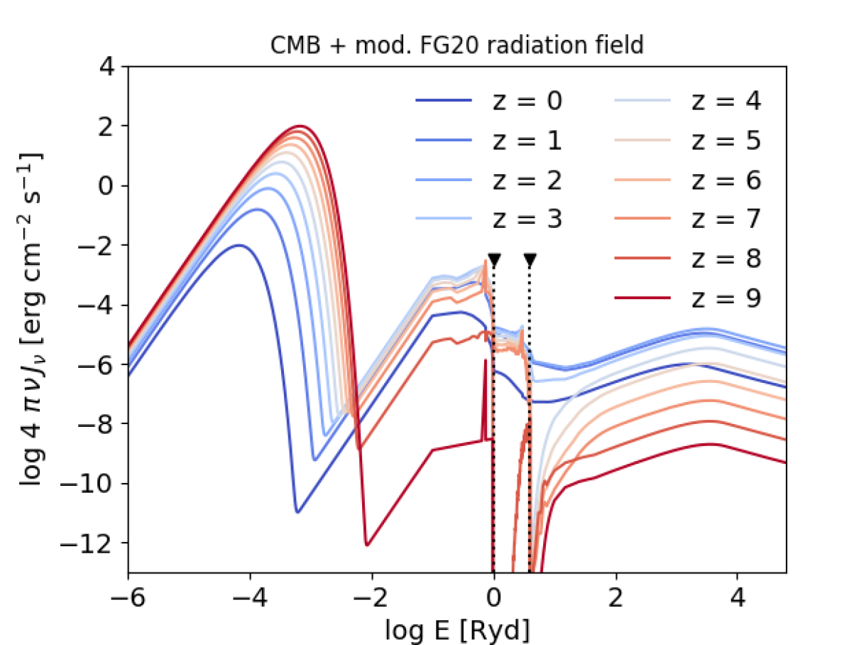
Obrázek 3: The incident background radiation field present in all tables for different redshifts consists of the CMB (lowest energy bump) and the modified FG20 UV / X-ray background (see Sec. 2.2.1 and Appendix B for details). The vertical dotted lines indicate the H i (left) and He ii (right) ionization energies. Before reionization is complete, the UVB is reduced for $z>3$ ($z>7.2$) at energies above the He ii (H i) ionization energy. See Fig. 23 for a comparison to the original FG20 UVB.

2.2.2 Interstellar radiation field

For gas in the ISM, the diffuse ISRF from nearby stars can be stronger than the UVB. As discussed in the introduction, this type of radiation field can be described by its intensity as well as an undefined number of parameters that model its spectral shape.

Here, we fix the shape of the ISRF to that described in Black (1987) for the Milky Way Galaxy and normalize it based on the reference column density $N_{\mathrm{ref}}$, which only depends on the gas density and temperature (Eq. 6). This is motivated by the observed star formation law and it avoids an extension of the tables to additional dimensions describing the ISRF and allows their use in simulations where the strength of the ISRF is not directly traced.

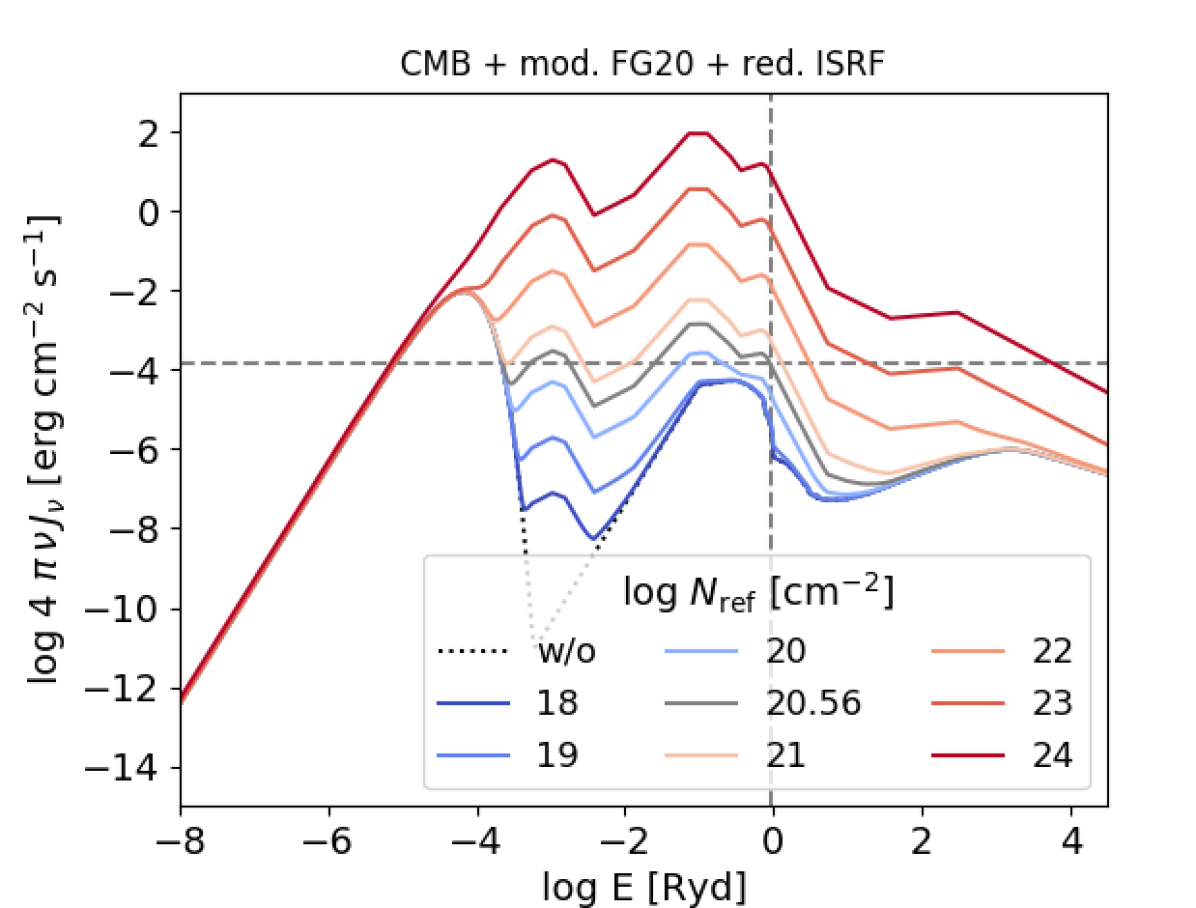
Obrázek 4: Total incident radiation field at $z=0$, including the CMB, the UVB and the local ISRF for different reference column densities, $N_{\mathrm{ref}}$. The shape of the ISRF is from Black (1987) and its intensity scales with $N_{\mathrm{ref}}^{1.4}$ as suggested by the Kennicutt-Schmidt law (see Eq. 13). The intensity of the total radiation field is defined at 1000 Å (vertical dashed line), with $4\pi\nu J_{\nu}=1.4\times 10^{-4}\,\mathrm{erg}\,\mathrm{cm}^{-2}\,\mathrm{s}^{-1}$ (horizontal dashed line) for $\log N_{\mathrm{ref}}=\log N_{\mathrm{H,0}}[\,\mathrm{cm}^{-2}]=20.56$ (scaling as in Eq. 13 with $\log R=-1$). For $\log N_{\mathrm{ref}}[\,\mathrm{cm}^{-2}]<18$, the total radiation field converges to the FG20 plus CMB radiation field (black dotted line, see Fig. 3 for other redshifts) for most energies.

In the case of a universal initial mass function (IMF), the rate at which OB stars are formed is proportional to the local SFR and the normalization of the Black (1987) radiation field is therefore assumed to scale with the SFR surface density $\Sigma_{\mathrm{SFR}}$ as

$$\log\frac{J}{J_{\mathrm{0}}}=\log\Sigma_{\mathrm{SFR}}-\log\Sigma_{\mathrm{SFR,0}}+\log R\,,$$ (9)

where $R$ is a renormalization factor. The solar neighbourhood values $J_{0}=4.4\times 10^{5}\,\mathrm{photons}\,\mathrm{cm}^{-2}\,\mathrm{s}^{-1}\,\mathrm{sr}^{-1}\,\mathrm{eV}^{-1}$ (or $4\pi\nu J_{\nu,0}=1.4\times 10^{-3}\,\mathrm{erg}\,\mathrm{cm}^{-2}\,\mathrm{s}^{-1}$) defined at a wavelength of 1000 Å (Black, 1987) and $\Sigma_{\mathrm{SFR,0}}=10^{-3}\,\mathrm{M}_{\odot}\,\mathrm{yr}^{-1}\,\mathrm{kpc}^{-2}$ (Bonatto & Bica, 2011) are used to normalise the ISRF (see Table 4 for an overview of solar neighbourhood quantities used in this work).

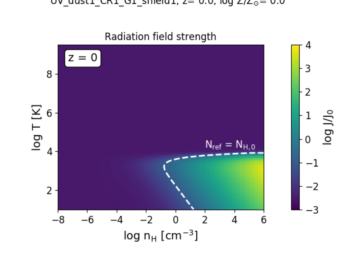
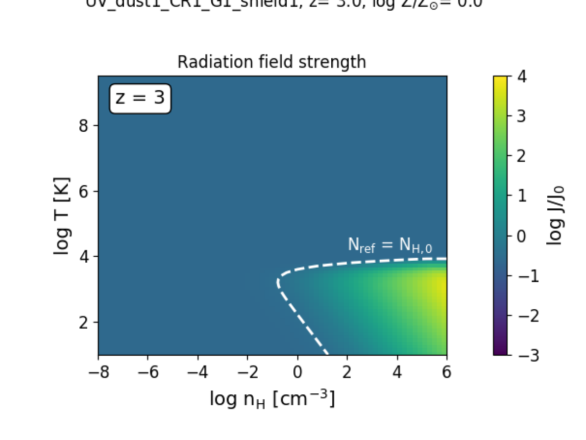
Obrázek 5: Total radiation field intensity defined at 1000 Å  relative to the MW value of $J_{\mathrm{0}}$ (see Table 4) at $z=0$ (top panel) and $z=3$ (bottom panel) for table UVB_dust1_CR1_G1. The radiation field is dominated by the ISRF at high densities and temperatures $\lesssim 10^{4}\,\,\mathrm{K}$ (with $\log J/J_{\mathrm{0}}\propto 1.4\times\log\Sigma_{\mathrm{SFR}}$) and smoothly transitions to the redshift-dependent UVB for higher temperatures and towards low densities. For reference, the dashed line indicates where $N_{\mathrm{ref}}=N_{\mathrm{H,0}}$ (MW value, see Table 4). Figures made with provided gui.

We assume that the SFR surface density $\Sigma_{\mathrm{SFR}}$ follows the observed Kennicutt-Schmidt relation (Kennicutt, 1998):

$$\Sigma_{\mathrm{SFR}}=A\left(\frac{\Sigma_{g}}{\mathrm{M}_{\odot}\,\mathrm{pc}^{-2}}\right)^{n}\,,$$ (10)

with $A=1.515\times 10^{-4}\,{\mathrm{M}}_{\odot}\,\mathrm{yr}^{-1}\,\mathrm{kpc}^{-2}$ and $n=1.4$. The amplitude $A$ has been decreased to account for a Chabrier (2003) IMF. These are the same values as used in the EAGLE simulations (Schaye et al., 2015) for which a similar scaling of the ISRF was used in Lagos et al. (2015) to compute molecular fractions. The gas surface density for a SFR of $\Sigma_{\mathrm{SFR,0}}$ is therefore

$$\Sigma_{\mathrm{g,0}}=3.85\,{\mathrm{M}}_{\odot}\,\mathrm{pc}^{-2}\,.$$ (11)

As the gas surface density is expressed as a total hydrogen column density in the tables, $\Sigma_{\mathrm{g,0}}$ is re-written as

$$N_{\mathrm{H,0}} =3.65\times 10^{20}\,\,\mathrm{cm}^{-2}\quad\mathrm{or}\quad\log N_{\mathrm{H,0}}[\,\mathrm{cm}^{-2}]=20.56\,,$$ (12)

using $X=0.7563$ as for the column density in Sec. 2.1. The final scaling of the ISRF based on $N_{\mathrm{ref}}$ is

$$\log\frac{J}{J_{\mathrm{0}}}= 1.4\times\left(\log N_{\mathrm{ref}}-\log N_{\mathrm{H,0}}\right)+\log R$$ (13)

$$\mathrm{dataset:}\,\texttt{RadField}$$

with a photoionization rate $\Gamma_{\mathrm{phot}}$ of

$$\log\frac{\Gamma_{\mathrm{phot}}}{\Gamma_{\mathrm{phot,0}}}=1.4\times\left(\log N_{\mathrm{ref}}-\log N_{\mathrm{H,0}}\right)+\log R\,.$$ (14)

where $R$ is the renormalization constant as in Eq. 9, $\Gamma_{\mathrm{phot,0}}(\text{H\,{i}})=3.75\times 10^{-11}\,\mathrm{s}^{-1}$ for H i ionization, $\Gamma_{\mathrm{phot,0}}(\text{He\,{i}})=3.10\times 10^{-12}\,\mathrm{s}^{-1}$ for He i and $\Gamma_{\mathrm{phot,0}}(\text{He\,{ii}})=1.43\times 10^{-14}\,\mathrm{s}^{-1}$ for He ii ionization.

For an unscaled Black (1987) radiation field ($\log R=0$), the molecular hydrogen fraction $f_{\mathrm{H2}}$ rises above 10 per cent only for neutral hydrogen column densities of $N_{\text{H\,{i}}}+2N_{\mathrm{H2}}\gtrsim 10^{21}\,\,\mathrm{cm}^{-2}$ for the thermal equilibrium temperature, which is inconsistent with observations. In addition, low-metallicity gas does not significantly cool below $10^{4}\,\mathrm{K}$ at any redshift. Renormalising the ISRF and the CR rate by a factor of 1/10 ($\log R=-1$) alleviates these tensions and the thermal equilibrium properties are in much better agreement with observations. This mismatch between the ISRF and the observed H₂ fractions has been found in previous work, where the H₂ formation rate on dust grains has to be boosted for a radiation field of 2.3 $J_{0}$ to reproduce the observations (e.g. Gnedin et al., 2009, Gnedin & Kravtsov, 2011, Gnedin & Draine, 2014). They relate this boost factor to the clumping factor $C_{\rho}$ and calibrate their model to this free parameter. This would account for unresolved higher density gas with higher molecule fractions. They find that clumping factors between $C_{\rho}\approx$ 10 and 30 are necessary to reproduce the observed H i - H₂ in the MW.

As cloudy solves a chemical network including several hundred molecules and atomic species, artificially increasing the formation rate of $H_{\mathrm{2}}$ by a factor that is a free parameter is neither practical nor self-consistent. In this case, decreasing the radiation field is a more reasonable approach. Note also that the assumed scaling of the ISRF with the star formation surface density may overestimate the radiation field. A higher $\Sigma_{\mathrm{SFR}}$ is linked to stronger local shielding of the stellar sources and may lead to a larger star formation scale height, both of which would reduce the local ISRF.

Fig. 4 shows the fiducial input spectrum ($\log R=-1$) at $z=0$ for different column densities $\log N_{\mathrm{ref}}$. For very small values of $N_{\mathrm{ref}}$, the UVB/CMB radiation field (black dotted line) dominates for $\log E\,[\mathrm{Ryd}]\lesssim-4$ and $\log E\,[\mathrm{Ryd}]\gtrsim-2$ and the intensity of the total radiation field in this energy range therefore becomes independent of the density and temperature. This transition depends on the intensity of the UVB and therefore on the redshift (see Fig. 5).

2.2.3 Before reionization

We apply the ISRF scaling $J\propto N_{\mathrm{ref}}^{1.4}$ at all column densities, so also at column densities lower than expected for the ISM. After reionization this is not a problem, because the UVB dominates over the ISRF at low densities. However, before reionization the ionizing radiation of distant galaxies is absorbed close to the source, while local radiation fields, such as the ionizing radiation from nearby stars (Sec. 2.2.2) remain unaffected. As the local radiation field is not attenuated, its contribution can even become dominant at low column / volume densities ($\log n_{\mathrm{H}}[\,\mathrm{cm}^{-3}]\lesssim-5$), which would not be part of the ISM and should therefore not be exposed to the ISRF. In order to avoid artificial gas heating, the ISRF normalization is drastically reduced compared to the reference value from $\log n_{\mathrm{H}}[\,\mathrm{cm}^{-3}]=-2$ to $-6$ with a similar asymptotic function as in Eq. 6:

$$\log(J/J_{\mathrm{0}})_{z>\mathrm{z_{reioniz}}}= \log(J/J_{\mathrm{0}})_{\mathrm{min}}-\frac{\log(J/J_{\mathrm{0}})_{\mathrm{min}}-\log J/J_{\mathrm{0}}}{1+e^{-2(\log n_{\mathrm{H}}[\,\mathrm{cm}^{-3}]+4)}}$$ (15)

$$\mathrm{or:}$$

$$\log(J/J_{\mathrm{0}})_{z>\mathrm{z_{reioniz}}}= \log(J/J_{\mathrm{0}})_{\mathrm{min}}-\frac{\log(J/J_{\mathrm{0}})_{\mathrm{min}}-\log J/J_{\mathrm{0}}}{1+c_{\mathrm{J}}n_{\mathrm{H}}^{k_{\mathrm{J}}}}$$

where $k_{\mathrm{J}}=-2/\ln(10)$ and $c_{\mathrm{J}}=e^{-8}$ regulate the steepness and position of the asymptotic transition to $\log(J/J_{\mathrm{0}})_{\mathrm{min}}=-20$. Without this extra scaling the radiation field would not converge to the (modified) FG20 background radiation for very low densities. Note, that this additional scaling is only necessary for $z>7.5$ as the photo-ionization rate of the UVB dominates that of the ISRF for lower redshifts at these densities.

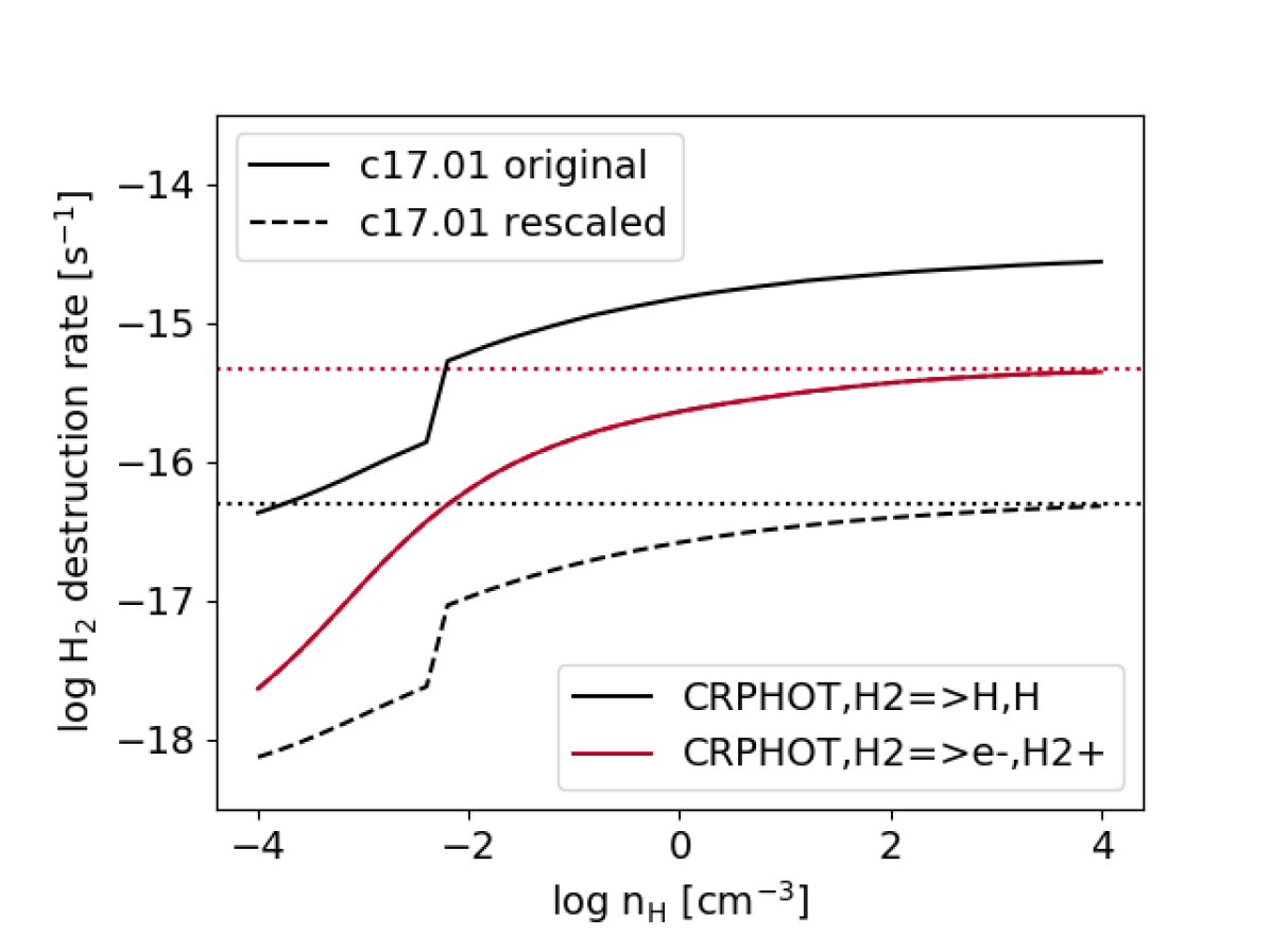
Obrázek 6: The H₂ destruction rates by cosmic rays for H₂ dissociation (“CRPHOT,H2=$>$H,H", black lines) and ionization (“CRPHOT,H2=$>$e-,H2+", red lines). In cloudy v17.01 (solid lines), the ionization rate converges to the input secondary ionization rate of $4.6\times 10^{-16}\,\mathrm{s}^{-1}$ (red, dotted line) but the dissociation rate is a factor of $\approx 6$ higher. In this work we rescale the rate for the reaction “CRPHOT,H2=$>$H,H"(dashed line) so that it converges to $5\times 10^{-17}\,\mathrm{s}^{-1}$ (black, dotted line) for high densities, the value expected from the UMIST database (see text for details).

2.3 Cosmic rays

Cosmic rays (CRs) are charged particles accelerated to high energies by diffuse shock acceleration in supernova remnants (Bell, 2004). Their production rate is therefore expected to be proportional to the rate of SNe and furthermore, for a constant IMF, to the SFR. This is supported by observations of starburst galaxies, where the CR rate is several orders of magnitude higher than locally in the MW Galaxy (e.g. Suchkov et al., 1993; Veritas Collaboration et al., 2009).

Analogously to the scaling of the ISRF intensity (Sec. 2.2.2), the H i CR ionization rate $\zeta_{\mathrm{CR}}$ is set to

$$\log\zeta_{\mathrm{CR}}\,[\mathrm{s}^{-1}]= \log\zeta_{\mathrm{CR,0}}+1.4\times\left(\log N_{\mathrm{ref}}-\log N_{\mathrm{H,0}}\right)+\log R$$ (16)

$$\mathrm{dataset:}\,\texttt{CosmicRayRate}$$

where $\zeta_{\mathrm{CR,0}}=2\times 10^{-16}\,\mathrm{s}^{-1}$ is the mean CR ionization rate of neutral hydrogen in local, diffuse clouds (Indriolo et al., 2007) and $\log R$ is the same renormalization constant as in Eq. 13 (we use $\log R=-1$ for the fiducial model).

We use the large cloudy model for the H₂ molecule (described in Shaw et al., 2005) which includes several thousand levels for the H₂ molecule. The H₂ ionization rate is therefore not constant but depends for example on the gas density (see the red solid line in Fig. 6). For high densities the H₂ destruction rate by cosmic rays due to H₂ ionization (labelled “CRPHOT,H2=$>$e-,H2+" in cloudy) converges to the input value of $4.6\times 10^{-16}\,\mathrm{s}^{-1}$ (red dotted horizontal line), following the ratio between H i and $\mathrm{H}_{\mathrm{2}}$ ionization rates from Glassgold & Langer (1974). According to the UMIST database (McElroy et al., 2013), the ratio between the rates for H₂ destruction by ionization and dissociation (labelled “CRPHOT,H2=$>$H,H" in cloudy) is 0.108, and the dissociation rate is therefore expected to converge towards $5\times 10^{-17}\,\mathrm{s}^{-1}$ (black, dotted horizontal line). In cloudy 17.01, the dissociation rate is a factor of 6 higher than the ionization rate (black solid line). We therefore rescale this rate to converge towards the expected value of $5\times 10^{-17}\,\mathrm{s}^{-1}$ (black dashed line) for high densities. This is more consistent with other chemical network codes, such as chimes (Richings et al., 2014a, b) that use the UMIST values and leads to higher $\mathrm{H}_{\mathrm{2}}$ fractions, in better agreement with observations (see Sec. 5.1).

The high H₂ dissociation rate in cloudy is caused by the assumed mean kinetic energy of the secondary electrons of 20 eV. For this energy the cross section for H₂ dissociation is at a maximum (Dalgarno et al., 1999). Future versions of cloudy will use a mean kinetic energy of 36 eV, more representative for the broad range of energies of secondary electrons, and this rescaling will not be necessary anymore (see Shaw et al., 2020 for details).

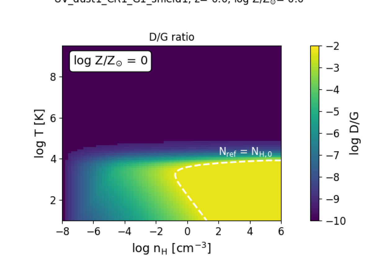
Obrázek 7: Assumed dust-to-gas mass ratio for solar metallicity. For $N_{\mathrm{ref}}>N_{\mathrm{H,0}}$ (higher density, lower temperature than the white dashed contour that indicates $N_{\mathrm{ref}}=N_{\mathrm{H,0}}$) the dust-to-metal mass ratio is constant while for lower densities and higher temperatures the dust content is reduced (Eq. 18). Figure made with provided gui.

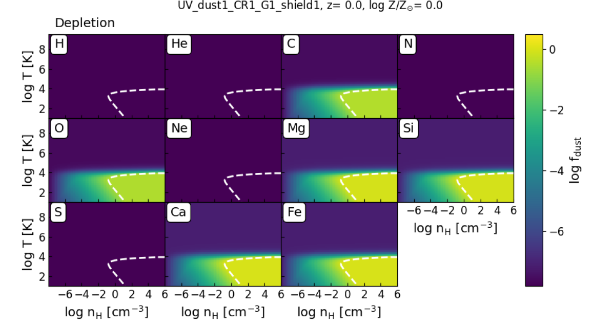
Obrázek 8: Metal depletion for all 11 tabulated elements. The color code shows the fraction of atoms of a given element that is locked into dust grains. Note the constant depletion for $N_{\mathrm{ref}}>N_{\mathrm{H,0}}$ (white dashed contour indicates $N_{\mathrm{ref}}=N_{\mathrm{H,0}}$) and the scaling with $N_{\mathrm{ref}}^{1.4}$ towards lower densities (Eq. 19). Figure made with provided gui.

2.4 Metallicity and dust

One of the table dimensions is the gas metallicity $Z$ in units of solar metallicity ${\mathrm{Z}}_{\odot}$, which ranges from $\log Z/{\mathrm{Z}}_{\odot}=-4$ to $0.5$ in steps of 0.5 dex (see Table 2). The abundances of all elements other than hydrogen and helium are scales with metallicity relative to their solar values (Table 3). For primordial abundances, an additional metallicity bin is added ($\log Z/{\mathrm{Z}}_{\odot}=-50$), using the primordial helium abundance $(n_{\mathrm{He}}/n_{\mathrm{H}})_{\mathrm{prim}}=0.08246$ (Planck Collaboration et al., 2016). To obtain a smooth transition between zero and solar metallicities, the helium abundance is linearly interpolated in between

$$\left(\frac{n_{\mathrm{He}}}{n_{\mathrm{H}}}\right)_{Z}=\left[\left(\frac{n_{\mathrm{He}}}{n_{\mathrm{H}}}\right)_{{\mathrm{Z}}_{\odot}}-\left(\frac{n_{\mathrm{He}}}{n_{\mathrm{H}}}\right)_{\mathrm{prim}}\right]\left(\frac{Z}{{\mathrm{Z}}_{\odot}}\right)+\left(\frac{n_{\mathrm{He}}}{n_{\mathrm{H}}}\right)_{\mathrm{prim}}$$ (17)

with $(n_{\mathrm{He}}/n_{\mathrm{H}})_{\odot}=0.0851$ (Asplund et al., 2009). The tables contain various datasets with information about the used abundance ratios (see Sec. 4.1.2).

The primordial abundance set in cloudy does not only include hydrogen and helium, but also traces of lithium and beryllium. Their minor cooling contribution explains why the metal cooling rate can be non-zero for primordial abundances.

2.4.1 Dust

We include the “Orion” grain set from cloudy. For solar metallicity, this grain set has a default dust-to-gas mass ratio of $(D/G)_{0}=5.6\times 10^{-3}$ and the relation between the extinction $A_{V}$ and the total hydrogen column density $N_{\mathrm{H}}$ is $\left(A_{V}/N_{\mathrm{H}}\right)=5.54\times 10^{-22}\,\mathrm{mag\,cm}^{2}$. The grain distribution with sizes between 300 and 2500 Å consists of both graphites and silicates and matches the extinction observed in Orion. In addition to dust grains, also polycyclic aromatic hydrocarbons (PAHs, with a power-law size distribution from Abel et al., 2008) are included as they contribute to photoelectric heating, collisional processes, and stochastic heating. As PAHs are destroyed in ionised gas by ionising photons and get depleted onto larger grains in molecular gas, their abundance is set to scale with the atomic neutral hydrogen fraction $n_{{\text{H\,{i}}}}/n_{\mathrm{H}}$ in cloudy.

A constant dust-to-metal ratio for ISM gas with $N_{\mathrm{ref}}>N_{\mathrm{H,0}}$ is assumed. As for this solar neighbourhood dust-to-metal ratio, some elements (e.g. Mg, Si, Ca, Fe) are already almost completely depleted on dust grains, higher dust-to-metal ratios would not be consistent. For lower reference column densities, a similar scaling as for the ISRF and the CR rate is used. The dust-to-gas mass ratio $D/G$ is then

$$\log D/G= \log Z/{\mathrm{Z}}_{\odot}+\log(D/G)_{0}\,+$$ (18)

$$+\mathrm{min}\begin{cases}1.4\times\left(\log N_{\mathrm{ref}}-\log N_{\mathrm{H,0}}\right)&\\ 0\\ \end{cases}$$

$$\mathrm{dataset:}\,\texttt{DGratio}$$

For $N_{\mathrm{ref}}=N_{\mathrm{min}}$ grain physics is completely disabled, as even extremely low grain abundances can cause cloudy to become unstable for high temperatures (i.e. $T>10^{6}\,\,\mathrm{K}$). Here, dust grains would be destroyed by thermal sputtering on very short timescales (e.g. Tielens et al., 1994), but this process is not included in cloudy. Fig. 7 summarises the dust-to-gas ratio dependence on density and temperature. The option no qheat is a standard cloudy command to disable quantum heating. This was necessary for code stability.

2.4.2 Metal depletion

The abundances of the Sun, which define the solar abundances, differ from those of the local ISM. For some elements a large fraction of atoms are depleted onto dust grains and their abundance ratios measured in the gas phase are correspondingly reduced. If the gas phase abundance were set to solar and dust grains were added to the mix without depleting the gas phase, the total (dust + gas) abundances would become super-solar.

For each element $i$, the number fraction of atoms that are depleted on dust grains is $f_{\mathrm{dust,i}}$, while $f_{\mathrm{gas,i}}=1-f_{\mathrm{dust,i}}$ is the number fraction of atoms of element $i$ in the gas phase. The reference values for solar neighbourhood conditions $\log f_{\mathrm{dust,i}}^{\prime}$ are taken from table 4 of Jenkins (2009), corrected for the different solar abundances used in their work.

As we add dust grains with constant dust-to-metal mass ratio for $N_{\mathrm{ref}}\geq N_{\mathrm{H,0}}$ and scale their abundance with the star formation activity for $N_{\mathrm{ref}}<N_{\mathrm{H,0}}$ (Eq. 18), the dust depletion for each grid point with $N_{\mathrm{ref}}$ and for each element $i$ is

$$\log f_{\mathrm{dust,i}}= \log f_{\mathrm{dust,i}}^{\prime}+\mathrm{min}\begin{cases}1.4\times\left(\log N_{\mathrm{ref}}-\log N_{\mathrm{H,0}}\right)&\\ 0\\ \end{cases}$$ (19)

$$\mathrm{dataset:}\,\texttt{Depletion}$$

and Fig. 8 illustrates this scaling.

2.5 HD cooling

In the cloudy version used (17.01), deuterium chemistry is disabled by default, contrary to the information in the user manual. Tests with a coarser grid where the deuterium chemistry was specifically added through the command line input, revealed that cloudy aborts for an increased number of grid points due to non-convergence issues in the chemistry solver. We therefore do not use the HD cooling from cloudy but add it analytically, following the cloudy prescription as closely as possible.

As in cloudy v17, the cooling rate per HD molecule, $W_{\mathrm{HD}}[\mathrm{erg\,s^{-1}}]$, is taken from the fitting function provided by Flower et al. (2000). $W_{\mathrm{HD}}$ depends on the gas density and temperature and was calculated by Flower et al. (2000) for temperatures between $30$ and $3000\,\mathrm{K}$ and densities $n_{\mathrm{H}}\geq 1\,\,\mathrm{cm}^{-3}$. The cooling rate from HD per unit volume is

$$\Lambda_{\mathrm{cool,HD}}=n_{\mathrm{HD}}W_{\mathrm{HD}}\,\mathrm{erg\,cm^{-3}\,s^{-1}}$$ (20)

where $n_{\mathrm{HD}}[\,\mathrm{cm}^{-3}]$ is the number density of HD molecules. As done in earlier cloudy versions, the HD abundance is assumed to follow the abundance of H₂ with $n_{\mathrm{HD}}/n_{\mathrm{H2}}=D/H$, with the primordial deuterium abundance of $D/H=1.65\times 10^{-5}$ (Pettini & Bowen, 2001). The cooling rate $\Lambda_{\mathrm{cool,HD}}$ is extrapolated to lower densities to avoid a sharp transition at $n_{\mathrm{H}}=1\,\,\mathrm{cm}^{-3}$. As both $n_{\mathrm{HD}}$ and $W_{\mathrm{HD}}$ are lower for lower densities, $\Lambda_{\mathrm{cool,HD}}$ is negligible for these densities. For temperatures $>10^{4}\,\mathrm{K}$, $\Lambda_{\mathrm{cool,HD}}$ is set to zero, as $W_{\mathrm{HD}}$ increases super-linearly with temperature, which can lead to non-negligible HD cooling rates, even if the HD abundance is very low.

At low redshift the HD cooling rate is only important for very low metallicities and very high densities (it contributes between 10 and 50 per cent of the total cooling rate for $\log Z/{\mathrm{Z}}_{\odot}<-3$ and $\log n_{\mathrm{H}}[\,\mathrm{cm}^{-3}]>3$). For redshifts $z>8$ HD cooling dominates for temperatures below the CMB temperature ($T_{\mathrm{CMB}}(z=9)=27.3\,\mathrm{K}$). This is an artefact from the analytic fitting function that does not include a redshift dependence. It only affects the lowest temperature bins at the highest redshifts in the table, but the HD cooling rate should be used with care in this region of parameter space.

Tabulka 5: Overview of the models and the included processes. For the column “dust", an entry “yes" means that dust grains with a dust-to-gas ratio according to Eq. 18 are included and that individual elements are depleted onto dust grains as described by Eq. 19. Cosmic rays with a rate following Eq. 16 are included for runs labelled “yes" in the column “CR". In addition to the radiation from the CMB and the modified UVB from FG20 (all tables), an interstellar radiation field (Eq. 13) is added to the runs with “yes" in the column “ISRF". The shielding column density of Eq. 8 is used for self-shielded gas (“yes" in column “shielding"). The fiducial model “UVB_dust1_CR1_G1_shield1" is highlighted in italic. The symbol $\star$ indicates that the corresponding rate/intensity is uncalibrated ($\log R=0$ in Eqs. 13 and 16).

Model name	dust	CR	ISRF	shielding
Main tables, results discussed in Sec. 5
UVB_dust1_CR0_G0_shield0	yes	no	no	no
UVB_dust1_CR0_G0_shield1	yes	no	no	yes
UVB_dust1_CR1_G1_shield0	yes	yes	yes	no
UVB_dust1_CR1_G1_shield1	yes	yes	yes	yes
Additional tables available (not discussed here)
UVB_dust0_CR0_G0_shield0	no	no	no	no
UVB_dust1_CR1_G0_shield0	yes	yes	no	no
UVB_dust1_CR1_G0_shield1	yes	yes	no	yes
UVB_dust1_CR2_G2_shield0	yes	yes⋆	yes⋆	no
UVB_dust1_CR2_G2_shield1	yes	yes⋆	yes⋆	yes

3 Models

The fiducial model that we recommend for use in simulations is “UVB_dust1_CR1_G1_shield1" as it includes all processes discussed in Sec. 2 (a redshift-dependent metagalactic radiation field, Sec. 2.2, as well as a density- and temperature-dependent shielding column density, Sec. 2.1, interstellar radiation field, Sec. 2.2, cosmic ray rate, Sec. 2.3, and dust abundance, Sec. 2.4). In this model, both the CR rate as well the ISRF intensity scale with the pressure as expected for a self-gravitating disk following the Kennicutt-Schmidt star formation law, with a normalization that is reduced by 1 dex relative to the Black (1987) value for the Milky Way ($\log R=-1$ in Eqs. 13 and 16) in order to match the observed transition from atomic to molecular hydrogen (as will be discussed in Sec. 5.1). The unshielded counterpart of this model is “UVB_dust1_CR1_G1_shield0" where all other cloudy inputs, beside the shielding column density, are identical to model “UVB_dust1_CR1_G1_shield1".

For comparison of the fiducial model to models without CRs and ISRF, we include “UVB_dust1_CR0_G0_shield0" and “UVB_dust1_CR0_G0_shield1" the unshielded (“shield0") and self-shielded (“shield1") models, where the radiation field only depends on redshift and is the sum of the contributions from the CMB and the modified FG20 UVB (see Fig. 3). The unshielded table “UVB_dust1_CR0_G0_shield0" is conceptually comparable to the approach in W09, and can serve as an update to the W09 tables. The main differences are that we use a more recent cloudy version (here: v17.01, W09: v07.02), a different UV background (here: FG20, W09: Haardt & Madau 2001), and include dust grains for $\log T[K]\lesssim 5$. By construction, all other tables only differ from “UVB_dust1_CR0_G0_shield0" for $\log T[\,\mathrm{K}]\lesssim 5$. At higher temperatures (and also very low densities) all tables converge to this one, as all additionally included processes are relevant only for neutral and molecular gas.

Table 5 presents an overview of the models for which hdf5 files are provided. In addition to the above mentioned tables whose results will be further discussed in Sec. 5, additional tables are listed separately. We do not discuss them in detail here, as we do not recommend them for use in simulations, but they can be used to explore the impact of individual processes (e.g. a model with CRs but without ISRF: “UVB_dust1_CR1_G0_shield1" or a model without dust: “UVB_dust0_CR0_G0_shield0"). The model with the full ISRF intensity and CR rate ($\log R=0$ in Eqs. 13 and 16, “UVB_dust1_CR2_G2_shield1") is included as it motivates the renormalization of these two quantities.

For self-shielded models (“shield1") without CRs the individual cloudy runs can easily become unstable and crash as CRs are the only source of ionization in highly molecular regions. This is known behaviour, it is mentioned clearly in the cloudy user manual that: “the chemistry network will probably collapse if the gas becomes molecular but cosmic rays are not present". Grid points for which cloudy crashes (7,223 out of 3,089,636 or 0.2 per cent for model “UVB_dust1_CR0_G0_shield1" compared to 315 or 0.01 per cent for model “UVB_dust1_CR1_G0_shield1") can be identified with the hdf5 dataset GridFails (see Sec. 4.1) while for all other datasets the values for the crashed runs are interpolated in 2D (density, temperature) between their neighbouring grid points with successful runs.

4 Data products

The data products released with this publication are hdf5 files for the different models listed in Table 5. The main datafile of each model is available as “$<$modelname$>$.hdf5" (e.g. “UVB_dust1_CR1_G1_shield1.hdf5") and contains both input datasets (e.g. CR rate, radiation field intensity) as well as cloudy results (e.g. cooling and heating rates, ion fractions, $\mathrm{H}_{\mathrm{2}}$ and CO abundances). The content of these files is described in Sec. 4.1 and listed in Table 6.

For the model “UVB_dust1_CR1_G1_shield0" (unshielded) and the fiducial model “UVB_dust1_CR1_G1_shield1" (self-shielded), additional files are available with emissivities of 183 emission lines (“$<$modelname$>$_lines.hdf5"). These files are described in Sec. 4.2.

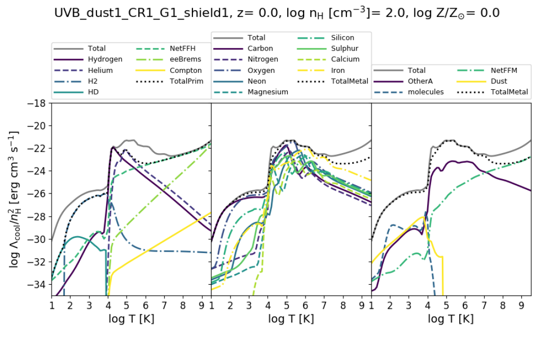
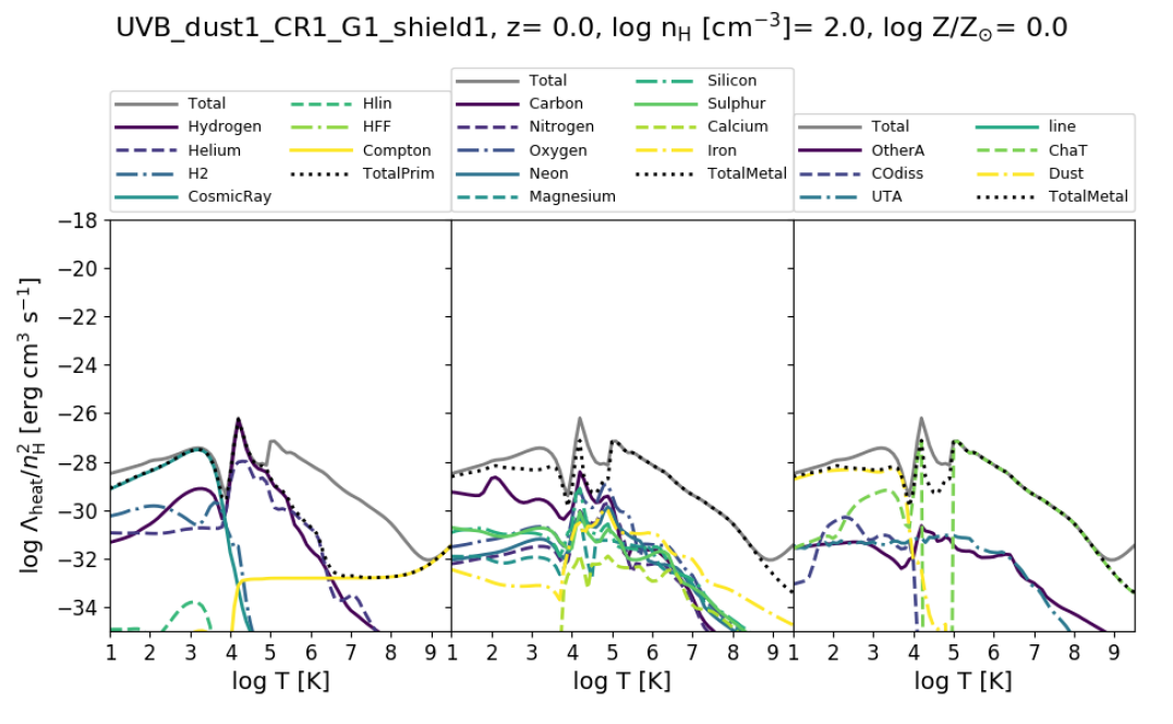
Obrázek 9: The top (bottom) panels show an example of the cooling (heating) contributions as listed in Table 9 (Table 10) from model UVB_dust1_CR1_G1_shield1 (see Table 5) for a gas density of $n_{\mathrm{H}}=100\,\,\mathrm{cm}^{-3}$, solar metallicity and at redshift 0. The components are split into primordial (left panel), atomic metal (middle panel) and the remaining metal processes (right panel). The black dotted line in each panel shows the total rate of the contribution of H and He (left panel) or from metals (middle and right panel) and the solid grey line in each panel indicates the total rate. The individual cooling (heating) processes are explained in Table 9 (Table 10). Figure made with provided gui.

4.1 Main hdf5 files: rates and fractions

The results for each model listed in Table 5 are stored in an hdf5 file that contains both the data as well as documentation. An overview of all datasets is given in Table 6 and additional information can be found in the attributes Dimension, Info and Unit of each dataset. We discuss a selection of entries that require more explanation below.

4.1.1 General structure

The hdf5 group /TableBins/ contains the values for each dimension already mentioned in Table 2 and the number of grid points in each dimension is stored in the hdf5 group /NumberOfBins/. A cloudy run was started for each redshift, temperature, metallicity, and density, which results in $N_{z}\times N_{T}\times N_{Z}\times N_{n_{\mathrm{H}}}=46\times 86\times 11\times 71=3,089,636$ individual cloudy runs per table.

Many hydrodynamic solvers do not use the gas temperature, $T$, but the internal energy per unit mass, $U$, as their main hydro variable. Hence, to use cooling rates tabulated as a function of temperature, the internal energy first has to be converted into the gas temperature. The relation between $U$ and $T$ is non-linear at phase transitions (mainly $\mathrm{H}_{\mathrm{2}}$ - H i and H i - H ii), where both the mean particle mass $\mu$ and the ratio of specific heats $\gamma$ change rapidly. To improve the usability of the code, we provide all full data hypercuboids (Sec. 4.1.3) both as a function of temperature (hdf5 group: /Tdep/) and internal energy (hdf5 group: /Udep/). The dimension of the full grid in /Udep/ is $N_{z}\times N_{U}\times N_{Z}\times N_{n_{\mathrm{H}}}$ (with the internal energy replacing the temperature dimension) and the internal energy bins can be found in dataset: InternalEnergyBins. The hdf5 group /ThermEq/ does not include a temperature or internal energy dimension (therefore the dimensions are: $N_{z}\times N_{Z}\times N_{n_{\mathrm{H}}}$), as it contains the gas properties at their thermal equilibrium temperature (dataset: ThermEq/Temperature) defined at the last zone of the cloudy calculation. Note that by definition the net cooling rate (cooling - heating) is zero for the thermal equilibrium temperature.

Tabulka 6: Overview of all datasets stored in each hdf5 table. A dataset is labelled with the prefix ⁽ⁱⁿ⁾ if it contains cloudy input, and with ^(out) if it contains results of the cloudy calculations. Note that cloudy assumes chemical and ionization equilibrium. Column 2 shows the size and dimensions of each dataset: z (redshift), T (gas temperature), Z (gas metallicity), $n_{\mathrm{H}}$ (gas density), U (gas internal energy), E (individually tabulated elements), C (cooling channels), and H (heating channels). In general, all resulting properties refer to those in the last zone in the cloudy calculation. For hydrogen and CO, average fractions over the full column density are also stored. The suffix “Col" refers to the column density fraction and the suffix “Vol" refers to the volume density fraction at the last zone.

Dataset name	dimension	comment
Group: /TableBins/, table dimensions, see also Sec. 4.1.1
RedshiftBins	z (46)	Redshifts for the $z$ dimension
TemperatureBins	T (86)	Temperatures for the $\log T[\,\mathrm{K}]$ dimension (group: /Tdep/)
MetallicityBins	Z (11)	Metallicities for the $\log Z/{\mathrm{Z}}_{\odot}$ dimension
DensityBins	$n_{\mathrm{H}}$ (71)	Densities for the $\log n_{\mathrm{H}}[\,\mathrm{cm}^{-3}]$ dimension
InternalEnergyBins	U (191)	Internal energies for the $\log U[\mathrm{erg\,g}^{-1}]$ dimension (group: /Udep/)
Additional information, see also Sec. 4.1.2
ElementNamesShort	E (11)	Short identifier for individually traced elements (e.g. H, He, C,…)
ElementNames	E+1	Names of elements (incl. one entry for all other atoms)
ElementMasses	E+1	Masses in $u$ ($1u=1.66054\times 10^{-24}\,\mathrm{g}$) of elements listed in dataset: ElementNames
NumberOfIons	E	Number of ions for each of the individually traced elements
AbundanceHe	Z	He abundance for each metallicity (Eq. 17)
TotalExactMetallicity	Z	Exact metal mass fraction, differs slightly from MetallicityBins (see Sec. 4.1.2)
TotalAbundances	Z, E+1	Total (dust + gas) abundances $n_{i}/n_{\mathrm{H}}$ for each element $i$ at each metallicity
TotalMassFractions	Z, E+1	Total (dust + gas) mass fractions $M_{i}/M_{\mathrm{tot}}$ for each element $i$ at each metallicity
SolarMetallicity	-	Solar metallicity, ${\mathrm{Z}}_{\odot}$ = 0.0134 (Asplund et al., 2009)
JMW	-	Flux of the ISRF in the solar neighbourhood at 1000 Å ($1.36\times 10^{-3}$ erg cm-2 s-1)
IdentifierCooling	C (22)	String identifier for the different cooling channels
IdentifierHeating	H (24)	String identifier for the different heating channels
Groups: /Tdep/ ($\star=T$), /Udep/ ($\star=U$), /Thermeq/ ($\star$ dimension does not exist), see also Sec. 4.1.3
(in)CosmicRayRate	z, ${\star}$, Z, $n_{\mathrm{H}}$	Cosmic ray hydrogen ionization rate $\log\zeta_{\mathrm{CR}}[\mathrm{s}^{-1}]$
(in)DGratio	z, ${\star}$, Z, $n_{\mathrm{H}}$	Dust to gas mass ratio
(in)Depletion	z, ${\star}$, Z, $n_{\mathrm{H}}$, E	For each element the fraction $f_{\mathrm{dust}}$ that is depleted onto dust
(in)RadField	z, ${\star}$, Z, $n_{\mathrm{H}}$	Strength of the incident radiation field relative to the MW value (dataset: JMW)
(in)ShieldingColumn	z, ${\star}$, Z, $n_{\mathrm{H}}$	Exact shielding column $\log N_{\mathrm{H}}$ used in the cloudy run
(in)ShieldingColumnRef	z, ${\star}$, Z, $n_{\mathrm{H}}$	Reference shielding column $\log N_{\mathrm{ref}}$ (Eq. 6)
(out)Cooling	z, ${\star}$, Z, $n_{\mathrm{H}}$ , C	Cooling rate $\log\Lambda_{\mathrm{cool}}/n_{\mathrm{H}}^{2}$ for different cooling channels (see Table 9)
(out)Heating	z, ${\star}$, Z, $n_{\mathrm{H}}$ , H	Heating rate $\log\Lambda_{\mathrm{heat}}/n_{\mathrm{H}}^{2}$ for different heating channels (see Table 10)
(out)AVextend	z, ${\star}$, Z, $n_{\mathrm{H}}$	Extended-source extinction, total visual extinction in mag at 5500 Å
(out)AVpoint	z, ${\star}$, Z, $n_{\mathrm{H}}$	Point-source extinction, total visual extinction in mag at 5500 Å
(out)COFractionCol	z, ${\star}$, Z, $n_{\mathrm{H}}$	CO column density fraction $\log N_{\mathrm{CO}}/N_{\mathrm{H}}$
(out)COFractionVol	z, ${\star}$, Z, $n_{\mathrm{H}}$	CO volume density fraction $\log n_{\mathrm{CO}}/n_{\mathrm{H}}$
(out)ColumnDensitiesC	z, ${\star}$, Z, $n_{\mathrm{H}}$ , 3	Selected carbon column densities: $\log N_{\text{C\,{i}}}$, $\log N_{\text{C\,{ii}}}$, $\log N_{\mathrm{CO}}$
(out)ColumnDensitiesH	z, ${\star}$, Z, $n_{\mathrm{H}}$ , 3	Selected hydrogen column densities: $\log N_{\text{H\,{i}}}$, $\log N_{\text{H\,{ii}}}$, $\log N_{\mathrm{H2}}$
(out)ElectronFractions	z, ${\star}$, Z, $n_{\mathrm{H}}$ , E + 3	Free electron fraction $\log n_{\mathrm{e}}/n_{\mathrm{H}}$ from each individual element + prim, metal, total
(out)GammaHeat	z, ${\star}$, Z, $n_{\mathrm{H}}$	Ratio of specific heats $\gamma$, varies between 7/5 and 5/3
(out)GridFails	z, ${\star}$, Z, $n_{\mathrm{H}}$	0 if cloudy finished successfully, 1 if warnings or errors were present
(out)HydrogenFractionsCol	z, ${\star}$, Z, $n_{\mathrm{H}}$, 3	Column density H mass fractions: $\log N_{\text{H\,{i}}}/N_{\mathrm{H}}$, $\log N_{\text{H\,{ii}}}/N_{\mathrm{H}}$, $\log 2N_{\mathrm{H2}}/N_{\mathrm{H}}$
(out)HydrogenFractionsVol	z, ${\star}$, Z,$n_{\mathrm{H}}$, 3	Volume density H mass fractions: $\log n_{\text{H\,{i}}}/n_{\mathrm{H}}$, $\log n_{\text{H\,{ii}}}/n_{\mathrm{H}}$, $\log 2n_{\mathrm{H2}}/n_{\mathrm{H}}$
(out)HydrogenFractionsVolExtended	z, ${\star}$, Z, $n_{\mathrm{H}}$, 6	As HydrogenFractionsVol but also: $\log 2n_{\mathrm{H2^{+}}}/n_{\mathrm{H}}$, $\log 3n_{\mathrm{H3^{+}}}/n_{\mathrm{H}}$, $\log n_{\mathrm{H^{-}}}/n_{\mathrm{H}}$
(out)IonFractions/00hydrogen	z, ${\star}$, Z, $n_{\mathrm{H}}$, 2	Fractions of hydrogen atoms in each ionization state (gas-phase, see Eq. 27)
(out)IonFractions/01helium	z, ${\star}$, Z, $n_{\mathrm{H}}$, 3	As IonFractionsVol/00hydrogen, but for helium
(out)IonFractions/02carbon	z, ${\star}$, Z, $n_{\mathrm{H}}$, 7	As IonFractionsVol/00hydrogen, but for carbon
(out)IonFractions/03nitrogen	z, ${\star}$, Z, $n_{\mathrm{H}}$, 8	As IonFractionsVol/00hydrogen, but for nitrogen
(out)IonFractions/04oxygen	z, ${\star}$, Z, $n_{\mathrm{H}}$, 9	As IonFractionsVol/00hydrogen, but for oxygen
(out)IonFractions/05neon	z, ${\star}$, Z, $n_{\mathrm{H}}$, 11	As IonFractionsVol/00hydrogen, but for neon
(out)IonFractions/06magnesium	z, ${\star}$, Z, $n_{\mathrm{H}}$, 13	As IonFractionsVol/00hydrogen, but for magnesium
(out)IonFractions/07silicon	z, ${\star}$, Z, $n_{\mathrm{H}}$, 15	As IonFractionsVol/00hydrogen, but for silicon
(out)IonFractions/08sulphur	z, ${\star}$, Z, $n_{\mathrm{H}}$, 17	As IonFractionsVol/00hydrogen, but for sulphur
(out)IonFractions/09calcium	z, ${\star}$, Z, $n_{\mathrm{H}}$, 21	As IonFractionsVol/00hydrogen, but for calcium
(out)IonFractions/10iron	z, ${\star}$, Z, $n_{\mathrm{H}}$, 27	As IonFractionsVol/00hydrogen, but for iron
(out)MeanParticleMass	z, ${\star}$, Z, $n_{\mathrm{H}}$	Gas-phase mean particle mass $\mu$ in units of atomic mass unit $u$
(out)Tdep/U_from_T	z, T, Z, $n_{\mathrm{H}}$	Internal energy $\log U[\mathrm{erg\,g}^{-1}]$ for group /Tdep/
(out)ThermEq/U_from_T	z, Z, $n_{\mathrm{H}}$	Thermal equilibrium internal energy $\log U[\mathrm{erg\,g}^{-1}]$ for group /Thermeq/
(out)Udep/T_from_U	z, U, Z, $n_{\mathrm{H}}$	Temperature $\log T[\,\mathrm{K}]$ for group /Udep/
(out)ThermEq/Temperature	z, Z, $n_{\mathrm{H}}$	Thermal equilibrium temperature

4.1.2 Miscellaneous information

We select the 11 elements that contribute most to the thermal state of the gas (i.e. the dominant cooling contributions) and tabulate their properties individually and in more detail (listed in Table 3 and in dataset ElementNames). The remaining elements are combined into one entry where this is relevant (e.g. the cooling channel “OtherA", see Table 9). Several datasets contain information about these elements (i.e. their names, masses and number of ions) and their abundances.

As mentioned in Sec. 2.4 (Eq. 17), the helium abundance varies with metallicity to yield a smooth transition between the solar and primordial values. The values used for $n_{\mathrm{He}}/n_{\mathrm{H}}$ at each metallicity are stored in dataset AbundanceHe. The extra scaling of helium changes the helium mass Y which results in a slightly different metal mass fraction $Z=Z/(X+Y+Z)$ compared to the values from the dataset MetallicityBins, which were used to scale the metal abundances independently. The difference is very small ($<$ 0.03 dex), but for reference the exact metallicity values are stored in TotalExactMetallicity. This array can be used instead of MetallicityBins, but has the practical disadvantage that it is not exactly uniformly spaced in $\log Z$.

The dataset ElementMasses $m_{i}$ is added to allow the conversion between element abundances ($n_{i}/n_{\mathrm{H}}$) and mass fractions, $M_{i}/M_{\mathrm{tot}}=(n_{i}/n_{\mathrm{H}})\times m_{i}/[\sum_{i}(n_{i}/n_{\mathrm{H}})\times m_{i}]$. The last entry of ElementMasses is the average atomic mass of the remaining elements for solar abundances from Asplund et al. (2009).

All metallicities are tabulated relative to the solar metallicity ${\mathrm{Z}}_{\odot}$ and can be converted to absolute metallicities by multiplying them with the entry from the dataset SolarMetallicity. Similarly, the radiation field dataset RadField is normalised to the local value $J_{0}$, which is stored in the dataset JMW.

The datasets IdentifierCooling and IdentifierHeating contain the labels listed in columns 2 of Tables 9 and 10. They correspond to the final dimension of the datasets Cooling and Heating (see Sec. 4.1.3).

4.1.3 Full data hypercuboid

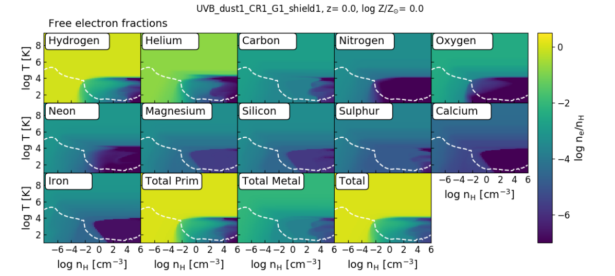
Obrázek 10: An example of the dataset ElectronFractions for table UVB_dust1_CR1_G1_shield1 for solar metallicity gas at redshift 0. The colour coding shows the free electron fraction $n_{\mathrm{e}}/n_{\mathrm{H}}$ in the last zone of the shielding column split up into contributions from individual elements, as well as the total contributions from hydrogen and helium (including electrons from hydrogen molecules, TotalPrim), from metals (TotalMetal) and the total electron fraction (including electrons from all molecules, Total). Figure made with provided gui.

There are three big groups in each hdf5 file that contain the same datasets but are tabulated in slightly different ways. In group /Tdep/ each grid point corresponds directly to a cloudy run with redshift, temperature, metallicity and density as inputs that remain constant throughout each 1D cloudy simulation. As already mentioned in Sec. 4.1.1, some hydrodynamic codes use the internal energy as the thermal variable instead of the gas temperature. For this case, using the datasets from group /Udep/ saves having to convert from $T$ to $U$, as the datasets now use the internal energy instead of the temperature dimension.

To create the datasets in group /Udep/, we first calculated the internal energy with

$$U[\mathrm{erg\,g}^{-1}]= \frac{1}{\gamma-1}\frac{k_{B}T}{\mu m_{u}}$$ (21)

$$\mathrm{dataset:}\,\texttt{Tdep/U\_from\_T}$$

with the Boltzmann constant $k_{B}=1.3806\times 10^{-16}\,\mathrm{erg\,K}^{-1}$ and the atomic mass unit $m_{u}=1.6605\times 10^{-24}\,\mathrm{g}$. Both the ratio of specific heats $\gamma$ and the mean particle mass $\mu$ vary within the table range. For $\mu$ we use the values from the dataset MeanParticleMass, which is a direct cloudy output. We approximate $\gamma$ by assuming it is dominated by the contributions from hydrogen and helium as

$$\gamma= \frac{5\left(n_{\text{H\,{i}}}+n_{\text{H\,{ii}}}+n_{\mathrm{He}}+n_{\mathrm{e}}\right)+7n_{\mathrm{H2}}}{3\left(n_{\text{H\,{i}}}+n_{\text{H\,{ii}}}+n_{\mathrm{He}}+n_{\mathrm{e}}\right)+5n_{\mathrm{H2}}}$$ (22)

$$\mathrm{dataset:}\,\texttt{GammaHeat}$$

assuring a smooth transition between $\gamma=5/3$ for monoatomic gas and $\gamma=7/5$ for molecular hydrogen (as done in the krome package, Grassi et al., 2014). In a second step, the properties of all datasets are interpolated onto fine, uniformly spaced bins in internal energy (dataset: TableBins/InternalEnergyBins).

The large phase-space covered by the tables is not uniformly populated by the gas resolution elements in a simulation. Typically gas will spend a disproportionally large fraction of its time close to thermal equilibrium. For all datasets, the group /ThermEq/ contains the properties at the thermal equilibrium temperature at the last cloudy zone (dataset: /ThermEq/Temperature). Occasionally, there are multiple equilibrium temperatures for a given density (at constant $z$ and $Z$). This occurs for example if an individual cooling contribution (e.g. molecular hydrogen) peaks around a given temperature while the heating rate stays roughly constant, which results in two thermal equilibrium tracks (at temperatures below and above the cooling peak). In this case (usually only for a narrow range in densities) we select the track that changes the equilibrium temperature the least, if the gas is moving to higher densities. The regions with multiple thermal equilibrium temperatures can be easily identified in a temperature - density plot of the net cooling rate (e.g with the provided gui). The minimum temperature in all tables is 10 K. If the cooling rate exceeds the heating rate at 10 K, we set $T_{\mathrm{eq}}=10\,\,\mathrm{K}$.

Input datasets:

Some of the datasets in Table 6 have the prefix ⁽ⁱⁿ⁾. These are properties that are not calculated by cloudy but are used as inputs. As they vary over different dimensions, we output their values during runtime as an independent check to verify that the scaling is implemented correctly.

Cooling and heating:

cloudy follows a large number of different cooling and heating channels. We combined them in the 20 cooling and 22 heating groups listed in Tables 9 and 10. In addition, the last two entries in this dimension are the total rates from processes including hydrogen and helium (labelled as: TotalPrim) and from processes including metals (TotalMetal). This allows one to calculate the rates faster for solar relative abundances by adding only the last two entries (for more details on how to use the tables, see Appendix A).

The heating and cooling labels from cloudy are listed in column 4 of Tables 9 and 10 and we refer to the cloudy documentation for more details on the individual processes. An example of the cooling and heating rates can be found in Fig. 9.

Vol and Col:

A cloudy calculation that includes self-shielding splits the gas shielding column into a varying number of zones with adaptive sizes. Each output property (labelled with ^(out) in Table 6) is defined at each zone throughout the gas column. In this work, every tabulated property refers to its value calculated at the last zone of the cloudy simulation. For self-shielded gas the last zone is the zone at the shielding column density and for unshielded gas the last zone is the only zone in the calculation.

If a phase transition occurs just before the last zone, the species fraction in the last zone can be very different from the species fraction integrated over the full shielding column. For the hydrogen and CO fractions we therefore store both values: $n_{\mathrm{x}}/n_{\mathrm{H}}$ (suffix: “Vol") at the last zone as well as $N_{\mathrm{x}}/N_{\mathrm{H}}$ (suffix: “Col") for the full shielding column.

In simulations, the shielding length $l_{\mathrm{sh}}=N_{\mathrm{sh}}/n_{\mathrm{H}}$ can be compared to the length scale of the resolution element $l_{\mathrm{sim}}$ to decide whether $n_{\mathrm{x}}/n_{\mathrm{H}}$ (for $l_{\mathrm{sim}}>l_{\mathrm{sh}}$) or $N_{\mathrm{x}}/N_{\mathrm{H}}$ (for $l_{\mathrm{sim}}<l_{\mathrm{sh}}$) is a better approximation. $n_{\mathrm{x}}/n_{\mathrm{H}}$ will only differ significantly from $N_{\mathrm{x}}/N_{\mathrm{H}}$ in small parts of the full table parameter space. For example for UVB_dust1_CR1_G1_shield1 $n_{\mathrm{H2}}/n_{\mathrm{H}}$ ($n_{\text{H\,{i}}}/n_{\mathrm{H}}$) differs by more than a factor of 2 from $N_{\mathrm{H2}}/N_{\mathrm{H}}$ ($N_{\text{H\,{i}}}/N_{\mathrm{H}}$) in less than 10 (1) per cent of the 3,089,636 entries.

Free electron fractions:

This dataset contains the number of free electrons per hydrogen atom $n_{\mathrm{e,X}}/n_{\mathrm{H}}$ for each individually traced element $X$. The number of electrons per gas phase atom of element $X$ is calculated from the fractions of atoms in ion stage $i$ with

$$\frac{n_{\mathrm{e,X,gas}}}{n_{\mathrm{X,gas}}}= \sum_{i=1}^{N_{\mathrm{ion,X}}}(i-1)\frac{n_{X,i}}{n_{X}}$$ (23)

(e.g. for He: $n_{\mathrm{e,He,gas}}/n_{\mathrm{He,gas}}=n_{\text{He\,{ii}}}/n_{\mathrm{He}}+2n_{\text{He\,{iii}}}/n_{\mathrm{He}}$). Accounting for the total abundance of element $X$ and depletion onto dust (for tables that include grains), the number of electrons per hydrogen atom from element $X$ is

$$\frac{n_{\mathrm{e,X}}}{n_{\mathrm{H}}}= \frac{n_{\mathrm{e,X,gas}}}{n_{\mathrm{X,gas}}}\underbrace{\frac{n_{\mathrm{X,gas}}}{n_{\mathrm{X}}}}_{\mathrm{1-f_{\mathrm{dust,X}}}}\frac{n_{\mathrm{X}}}{n_{\mathrm{H}}}$$ (24)

where $n_{\mathrm{X,gas}}$ is the gas phase number density and $n_{\mathrm{X}}$ the total (gas + dust) number density of element $X$. The contributions from ionized molecules are not included here, but for metals these are negligible. The last three entries in the element dimension are the total primordial electron fractions (including species $n_{\mathrm{H2}^{+}}$, $n_{\mathrm{H3}^{+}}$ and $n_{\mathrm{H}^{-}}$), the total fractions of free electrons from metals $n_{\mathrm{e,met}}/n_{\mathrm{H}}$ without molecules, and $n_{\mathrm{e,tot}}/n_{\mathrm{H}}$ from all atoms and molecules included in cloudy. Fig. 10 illustrates the individual entries for solar metallicity gas at redshift 0 (using table UVB_dust1_CR1_G1_shield1).

Splitting the electron fractions into individual elements allows users to combine these tables with a chemical network that follows the non-equilibrium evolution of a subset of elements (e.g. H and He). The free electrons from metals in self-shielded gas can be added to the network individually (see Appendix A.2).

Ion fractions:

An individual dataset containing the ion fractions of each element listed in Table 3 is included in every hdf5 file. The size of the last dimension in each ion fraction dataset (see Table 6) is the number of ions, given in the additional dataset NumberOfIons. For each element the ion fractions are defined as the number of atoms in each ionization state relative to the total number of atoms of this element in the gas phase (e.g. $n_{\text{H\,{i}}}/n_{\mathrm{H}}$). The sum of all ion fractions for an element does not add up to one if a non-negligible fraction of atoms are in molecules.

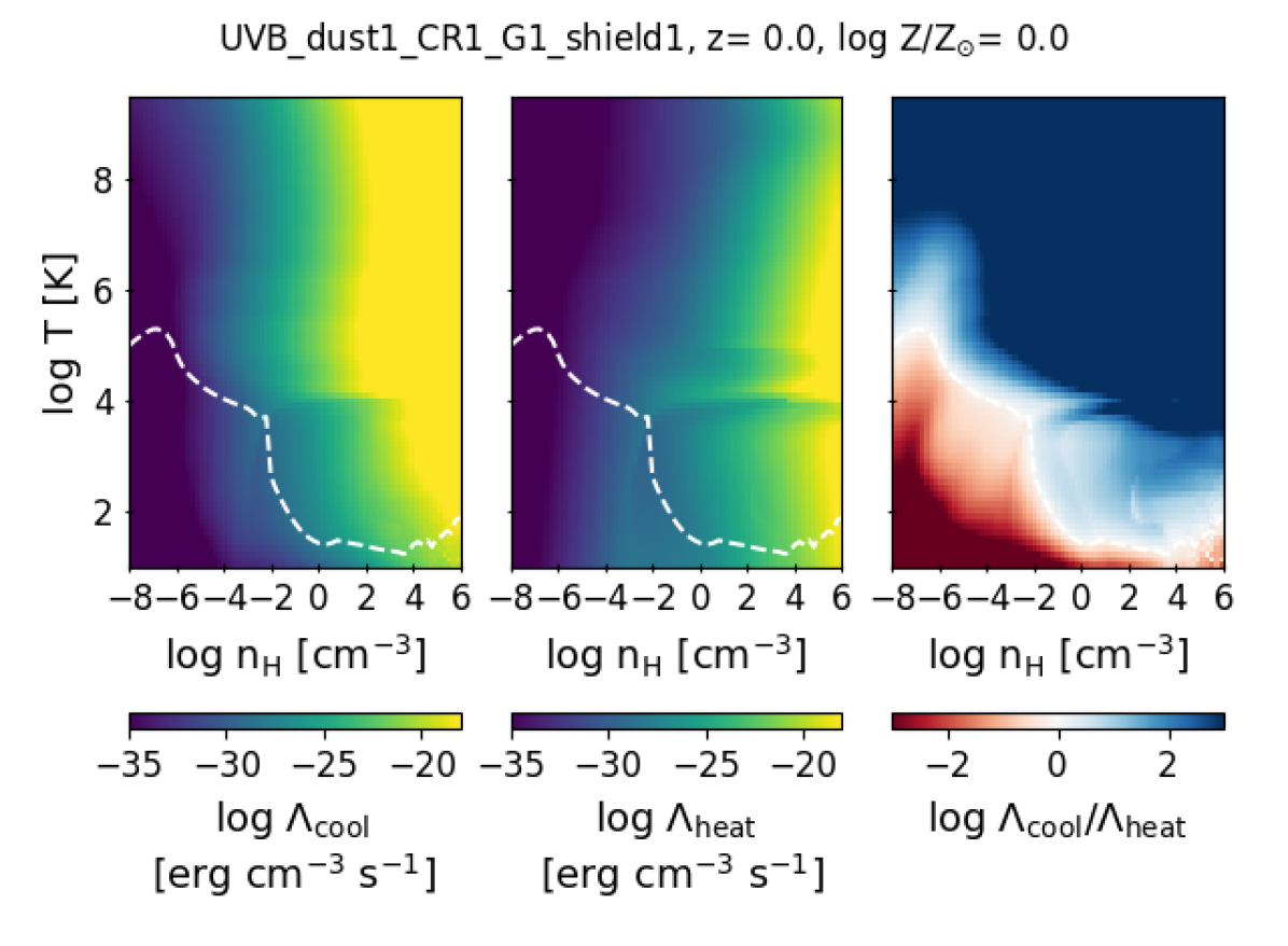
Obrázek 11: Cooling ($\Lambda_{\mathrm{cool}}$, left panel) and heating ($\Lambda_{\mathrm{heat}}$, middle panel) rate, as well as their ratio ($\Lambda_{\mathrm{cool}}/\Lambda_{\mathrm{heat}}$, right panel) for solar metallicity gas at $z=0$ from table UVB_dust1_CR1_G1_shield1. The white dashed line in each panel indicates the thermal equilibrium temperature (i.e. $\Lambda_{\mathrm{cool}}/\Lambda_{\mathrm{heat}}=1$). Figure made with provided gui.

4.2 Line emissivity hdf5 files:

For tables UVB_dust1_CR1_G1_shield0 and UVB_dust1_CR1_G1_shield1 we provide additional information on the emissivity of selected lines (see Table 7 and dataset: IdentifierLines) in a separate hdf5 file (“$<$modelname$>$_lines.hdf5"). The general file structure is the same as in the hdf5 files that contain the rates and species fractions (Sec. 4.1) as the emissivities are calculated for the same grid in redshift, metallicity, density and temperature.

For each line the hdf5 file contains the line emissivity in units of $\mathrm{erg}\,\mathrm{cm}^{-3}\,\mathrm{s}^{-1}$ that is leaving the illuminated side of the cloud (using the cloudy keyword “emergent"). The luminosity of a gas particle (or gas cell) in a simulation can be calculated with

$$L[\mathrm{erg}\,\mathrm{s}^{-1}]=\epsilon\frac{m_{\mathrm{gas}}}{\rho_{\mathrm{gas}}}\,,$$ (25)

following e.g. Bertone et al. (2010), where $m_{\mathrm{gas}}$ is the mass of the resolution element, $\rho_{\mathrm{gas}}$ is the gas density and $\epsilon$ is either the emissivity at the last zone ($\epsilon_{\mathrm{Vol}}$, dataset: EmissivitiesVol) or the average emissivity of the shielding column ($\epsilon_{\mathrm{Col}}$, dataset: EmissivitiesCol"). The emergent emissivities of the last zone ($\epsilon_{\mathrm{Vol}}$) are calculated by cloudy with the command “save lines emissivity" and the column averaged emissivity is calculated by dividing the emergent line intensity of the full shielding column (“save line list absolute") by the length of the shielding column. Analogous to the “Vol" and “Col" fractions from the main hdf5 file (discussed in Sec. 4.1.3), comparing the shielding length to the length scale of the resolution element can help decide which emissivity to choose.

Tabulka 7: Line identifiers and wavelengths for the lines in the line emission files (see Sec. 4.2). The wavelengths are in units of Å (A), cm (c), and $\mu$m (m). “Blnd" refers to a blended line with multiple components and is listed directly after its main component(s). The line with the cloudy identifier “Cool" at 1215Å is the contribution of collisional excitation to Ly$\alpha$ cooling.

Line	Wavelength	Line	Wavelength	Line	Wavelength	Line	Wavelength	Line	Wavelength
H 1	1025.72A	C 5	40.2678A	O 3C	4363.00A	Mg 9	62.7511A	Fe16	63.7110A
H 1	1215.67A	C 5	41.4721A	Blnd	4363.00A	Mg 9	72.0276A	Fe16	66.3570A
Cool	1215.67A	C 6	33.7372A	O 3	51.8004m	Mg10	63.2953A	Fe17	17.0510A
H 1	21.1207c	N 1	1200.00A	O 3	88.3323m	Mg11	9.16875A	Fe17	15.2620A
H 1	4861.33A	N 1	1200.22A	O 4	25.8832m	Mg12	8.42141A	Fe17	16.7760A
H 1	6562.81A	N 2	1084.56A	O 5	1218.34A	Si 2	1816.93A	Fe17	17.0960A
H 1	4340.46A	N 2	1084.58A	Blnd	1218.00A	Si 2	1817.45A	Fe18	16.0720A
H 1	4101.73A	N 2	1085.10A	O 6	1031.91A	Si 2	34.8046m	Fe18	93.9322A
H 1	920.963A	Blnd	1085.00A	O 6	1037.62A	Si 3	1206.50A	Fe22	11.7695A
H 1	923.150A	N 2	121.767m	Blnd	1035.00A	Si 3	1882.71A	Fe23	11.7370A
H 1	926.226A	N 2	205.244m	O 7	21.6020A	Blnd	1888.00A	Fe25	1.85040A
H 1	930.748A	N 2	6583.45A	O 7	21.8044A	Si 4	1393.75A	Fe26	1.78177A
H 1	937.804A	N 3	57.3238m	O 7	21.8070A	Si 4	1402.77A	CO	1300.05m
H 1	949.743A	N 3	991.000A	O 7	22.1012A	Blnd	1397.00A	CO	260.169m
H 1	972.537A	N 4	1486.50A	O 7	18.6270A	Si11	43.7501A	CO	2600.05m
He 2	1640.43A	Blnd	1486.00A	O 8	16.0067A	Si11	52.2913A	CO	289.041m
He 2	303.784A	N 5	1238.82A	O 8	18.9709A	Si12	40.9111A	CO	325.137m
C 1	1561.34A	N 5	1242.80A	Ne 2	12.8101m	Si12	44.1650A	CO	371.549m
C 1	1561.37A	Blnd	1240.00A	Ne 3	15.5509m	Si13	6.64803A	CO	433.438m
C 1	1561.44A	N 6	29.5343A	Ne 3	3868.76A	Si14	6.18452A	CO	520.089m
C 1	1656.27A	N 6	28.7870A	Ne 3	3967.47A	S 2	4068.60A	CO	650.074m
C 1	370.269m	N 7	24.7807A	Ne 4	2424.28A	Blnd	4074.00A	CO	866.727m
C 1	609.590m	O 1	145.495m	Blnd	2424.00A	S 3	18.7078m	H2	12.2752m
C 2	1335.00A	O 1	5577.34A	Ne 5	14.3228m	S 3	33.4704m	H2	17.0300m
Blnd	1335.00A	O 1	63.1679m	Ne 7	97.4960A	S 4	10.5076m	H2	28.2106m
C 2	157.636m	O 1	6300.30A	Ne 8	88.0817A	S 5	1199.14A	H2O	269.199m
C 2	2328.12A	O 1	6363.78A	Ne 8	98.1156A	Blnd	1199.00A	H2O	303.374m
Blnd	2326.00A	Blnd	6300.00A	Ne 8	98.2601A	S 6	933.380A	H2O	398.534m
C 3	1906.68A	O 2	3726.03A	Ne 8	770.410A	S 7	72.0290A	HCO+	480.147m
C 3	1908.73A	Blnd	3726.00A	Blnd	774.000A	S 7	72.6640A	HCO+	560.140m
Blnd	1909.00A	O 2	3728.81A	Ne 9	13.4471A	S 15	5.03873A	HCO+	840.150m
C 3	977.000A	Blnd	3729.00A	Ne 9	13.6987A	Ar 2	6.98337m	HNC	661.221m
C 3	977.020A	O 3	4958.91A	Ne10	12.1375A	Ar 9	49.1850A	HNC	826.492m
Blnd	977.000A	O 3	5006.84A	Mg 1	2852.13A	Ca 1	4226.73A	OH	119.202m
C 4	1548.19A	Blnd	5007.00A	Mg 2	2795.53A	Fe 2	2399.24A	OH	119.410m
C 4	1550.78A	O 3	4363.21A	Mg 2	2802.71A	Fe 2	25.9811m
Blnd	1549.00A	O 3R	4363.00A	Blnd	2798.00A	Fe 5	3891.28A

5 Example results: Thermal equilibrium

The full tables can be explored with the help of the provided gui. Here, we focus on the properties of gas close to the thermal equilibrium temperature at the last zone of the gas column.

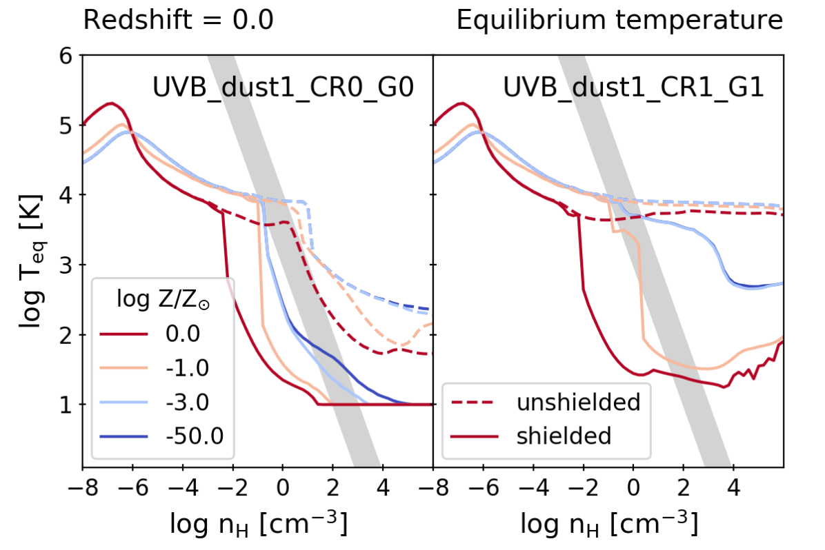
Obrázek 12: Thermal equilibrium temperatures for two different radiation fields, only CMB and UVB (UVB_dust1_CR0_G0, left panel) and including CRs and ISRF (UVB_dust1_CR1_G1, right panel) at redshift 0. The colours in each panel refer to different gas metallicities and the line styles indicate if the thermal equilibrium temperature is for unshielded (dashed lines, “_shield0") or self-shielded (solid lines, “_shield1") gas. The shaded area indicates ISM pressures of $3<\log P/k_{B}[\,\mathrm{K}\,\mathrm{cm}^{-3}]<4$ as observed in the solar neighbourhood by Jenkins & Tripp (2011).

An example for a density-temperature slice through the dataset hypercuboid for solar metallicity and $z=0$ is shown in Fig. 11. The plotted properties are the cooling rate ($\Lambda_{\mathrm{cool}}$, left panel), heating rate ($\Lambda_{\mathrm{heat}}$, middle panel), as well as the ratio between the two ($\Lambda_{\mathrm{cool}}/\Lambda_{\mathrm{heat}}$, right panel). The thermal equilibrium temperature, $T_{\mathrm{eq}}$, is defined as the temperature where $\Lambda_{\mathrm{cool}}/\Lambda_{\mathrm{heat}}=1$ (dashed, white line). This temperature is stored in dataset /ThermEq/Temperature and all properties in the group /ThermEq/ correspond to the relevant (for each $z$ and metallicity bin) thermal equilibrium temperatures.

$T_{\mathrm{eq}}$ typically serves as a lower temperature limit for ISM gas. Gas can have higher temperatures due to hydrodynamic processes (e.g. shocks) but temperatures below $T_{\mathrm{eq}}$ are rare as the heating rate typically dominates adiabatic losses at ISM densities. For densities around and below the cosmic mean $T_{\mathrm{eq}}$ is not a good proxy for the actual (quasi-)equilibrium temperature because here adiabatic cooling due to the Hubble expansion typically dominates over radiative cooling. More generally, when the radiative time scales exceed the Hubble time, the gas will not be able to achieve thermal equilibrium.

Fig. 12 displays an overview of the thermal equilibrium temperatures at $z=0$ for a selection of metallicities. Each panel shows two tables whose names start with the labels indicated in each panel. The dashed lines represent $T_{\mathrm{eq}}$ from the unshielded version (“_shield0"), while the solid lines are for $T_{\mathrm{eq}}$ including self-shielding (“_shield1"). For tables without an ISRF (left panel) even unshielded gas can cool down to temperatures below $10^{4}\,\,\mathrm{K}$ as soon as it becomes dense enough ($n_{\mathrm{H}}\gtrsim 1\,\mathrm{cm}^{-3}$). Including self-shielding moves the density of the transition from the warm ($T\approx 10^{4}\,\,\mathrm{K}$) to the cold ($T\ll 10^{4}\,\,\mathrm{K}$) gas phase to lower densities, depending on the gas metallicity.

Most of the ISM gas in the solar neighbourhood has thermal pressures of $3<\log P/k_{\mathrm{B}}[\,\mathrm{K}\,\mathrm{cm}^{-3}]<4$ (Jenkins & Tripp, 2011). The shaded areas in Fig. 12 indicate this range of pressures. For solar metallicity, the minimum equilibrium temperature of the cold phase is $\approx 30\,\,\mathrm{K}$ in table UVB_dust1_CR1_G1 while the warm phase (unshielded gas) has an equilibrium temperature of $\approx 10^{4}\,\,\mathrm{K}$. For tables including the reduced ISRF (right panel of Fig. 12), a multi-phase medium can be established between the unshielded and the self-shielded gas for high metallicity ($Z\geq 0.1\,{\mathrm{Z}}_{\odot}$) gas over a large range of densities.

The redshift dependence of $T_{\mathrm{Eq}}$ is shown in Fig. 13 for solar (left set of panels) and primordial abundances (right set of panels). As in Fig. 12, the left panel does not include the ISRF and $T_{\mathrm{Eq}}$ depends on redshift over the full density range. In the right panels of Fig. 13, which include the redshift-independent ISRF, the thermal equilibrium temperatures of different redshifts converge at high densities.

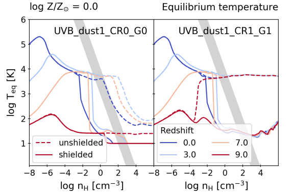
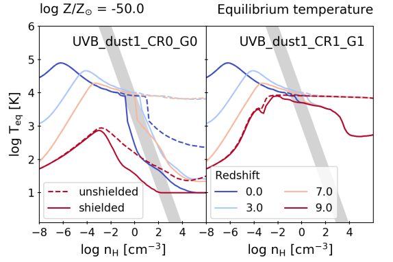
Obrázek 13: As. Fig. 12, but where each figure is for constant metallicity (left figure, solar metallicity; right figure, primordial abundances) and each line colour represents a different redshift.

$T_{\mathrm{Eq}}$ increases with density for the lowest densities in the tables (see Figs. 12 and 13). This relation is caused by the combination of a photo heating rate $\Lambda_{\mathrm{heat}}/n^{2}_{\mathrm{H}}$ that is independent of density for highly (photo-)ionized gas and Compton cooling rate $\Lambda_{\mathrm{cool,Compton}}/n^{2}_{\mathrm{H}}$ that increases with decreasing density. The redshift dependence at these densities is dominated by the steep dependence of Compton cooling with redshift. In practice the thermal equilibrium temperature from radiative processes is irrelevant for the lowest densities as the cooling time is longer than the Hubble time and adiabatic cooling (Hubble expansion) dominates over radiative cooling. At higher densities ($\log n_{\mathrm{H}}[\,\mathrm{cm}^{-3}]\gtrsim-5$ for $z=0$) hydrogen and helium recombination cooling dominates between $\log T[\,\mathrm{K}]\approx 4-6$ and $T_{\mathrm{Eq}}$ decreases with density.

The thermal equilibrium curves in Figs. 12 and 13 are reminiscent of the classical two phase structure of the neutral ISM, as described in Wolfire et al. (1995) (hereafter: W95). As it can be tempting to directly compare the thermal equilibrium curves from this work to those of W95, we discuss here the key differences in both the general approach as well as the interpretation of the results.

W95 describe the ISM densities where warm neutral ISM gas can be in pressure equilibrium with cold neutral gas. Based on the idea of a dense, cold gas cloud embedded in more tenuous, warm ($10^{4}\,\mathrm{K}$) gas, the pressure equilibrium is determined at the edge of the cold gas cloud. They assume that the ISRF is shielded by a constant column density ($N_{w}=10^{19}\,\mathrm{cm}^{-2}$ in their fiducial model), where $N_{w}$ is the typical column density of the warm medium. In this work, the shielding from the ISRF corresponds to the self-shielding of the cold gas cloud (i.e. from its edge to its centre). The shielding column $N_{\mathrm{sh}}$ therefore varies with the assumed size of the gas cloud, which is a function of gas density and temperature (or pressure, as $N_{\mathrm{sh}}\propto(n_{\mathrm{H}}T)^{0.5}$, see Sec. 2.1).

In addition to the varying shielding column, also the radiation field intensity and the CR rate change along the thermal equilibrium curves. Higher gas pressures lead to larger column densities which are observed to result in higher SFR densities and subsequently a stronger ISRF (see Sec. 2.2.2). While Wolfire et al. (2003) vary the ISRF to account for radial variations within the MW disk, the ISRF is constant with density for each of their equilibrium functions.

Fig. 14 illustrates the variations in the shielding column (top panels) and ISRF intensity (bottom panels). The coloured lines refer to the values at the thermal equilibrium temperatures for selected metallicities at $z=0$ and the grey horizontal lines show the fiducial values of the W95 model, with $\log N_{\mathrm{sh}}[\,\mathrm{cm}^{-2}]=19$ and the radiation field from Draine (1978) with $J_{\mathrm{D78}}=6.6\times 10^{5}\,\mathrm{photons}\,\mathrm{cm}^{-2}\,\mathrm{s}^{-1}\,\mathrm{sr}^{-1}\,\mathrm{eV}^{-1}$ and therefore $J_{\mathrm{D78}}/J_{0}=1.5$.

The column densities for the tables that include self-shielding span several orders of magnitudes for typical ISM densities ($n_{\mathrm{H}}\gtrsim 10^{-2}\,\,\mathrm{cm}^{-3}$). The radiation field spans an even larger range as $J\propto\Sigma_{\mathrm{SFR}}\propto{N_{\mathrm{sh}}}^{1.4}$. Higher pressure environments are therefore self-consistently exposed to more intense radiation fields.

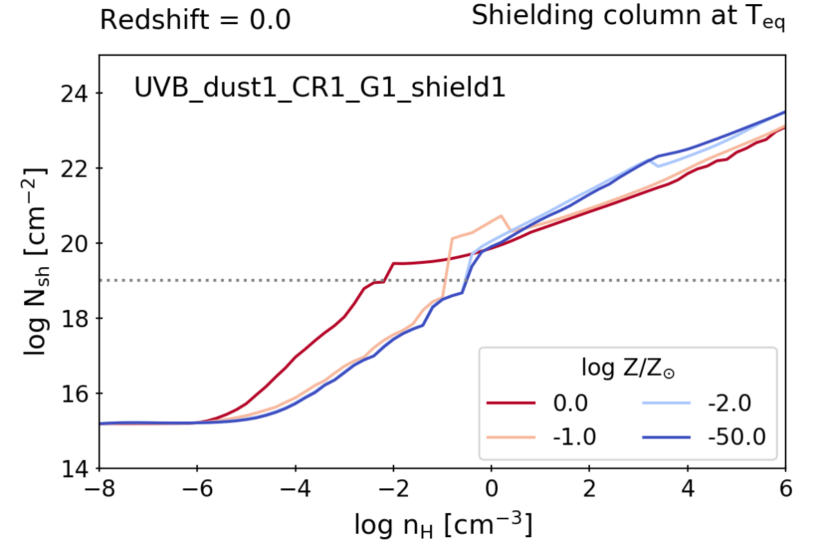
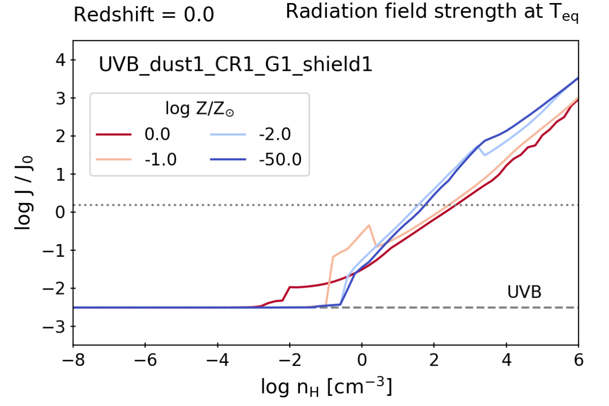
Obrázek 14: Shielding column (top panels) and ISRF strength (bottom panels) assuming the density-dependent thermal equilibrium temperature displayed in the right panel of Fig. 12 for self-shielded gas at $z=0$. The horizontal dotted lines refer to a constant column density of $\log N_{\mathrm{sh}}[\,\mathrm{cm}^{-2}]=19$ (top panel) and a constant radiation field intensity of $J_{\mathrm{D78}}=1.5J_{\mathrm{0}}$ (bottom panel), the default values used in W95. At low densities, where the UVB (dashed line, bottom panel) dominates the ISRF at 1000Å, the radiation field becomes independent of the density.

W95 and Wolfire et al. (2003) focus on the MW ISM and therefore assume solar metallicity. Recently, Bialy & Sternberg (2019) extended their model to lower metallicity gas and included molecular hydrogen heating and cooling processes. They found that a multi-phase medium requires higher pressure for lower metallicities if the ISRF is the same as that assumed in solar metallicity galaxies. For extremely low metallicities ($Z\lesssim 10^{-5}{\mathrm{Z}}_{\odot}$) and for a total CR ionization rate per hydrogen atom of $10^{-16}\,\mathrm{s}^{-1}$ they found that the ISM would be single-phase, as the equilibrium temperature changes smoothly from $\approx 10^{4}\,\mathrm{K}$ to $\approx 600\,\mathrm{K}$. Despite the above discussed differences, we find qualitatively similar behaviour for the thermal equilibrium temperatures of the recommended table UVB_dust1_CR1_G1_shield1. The colour scale in Fig. 15 shows the minimum pressure for unshielded (“_shield0") and shielded (“_shield1") gas to be in pressure equilibrium (where the former corresponds to the warm phase: $\log T_{\mathrm{warm}}[\,\mathrm{K}]>3.5$ and the latter to the cold phase: $\log T_{\mathrm{cold}}[\,\mathrm{K}]<3$). An overall trend with metallicity (i.e. lower metallicity - higher minimum pressure) is clearly visible for every redshift.

Note that for very low-metallicity gas ($\log Z/{\mathrm{Z}}_{\odot}\lesssim-2$) the lack of metal-line cooling keeps the temperature at $\gtrsim 800\,\mathrm{K}$, even for very high density gas ($n_{\mathrm{H}}=10^{6}\,\,\mathrm{cm}^{-3}$, see Fig. 12). This gas is mainly heated by CRs and by the vibrational and rotational energy of molecular hydrogen, as it absorbs UV photons.

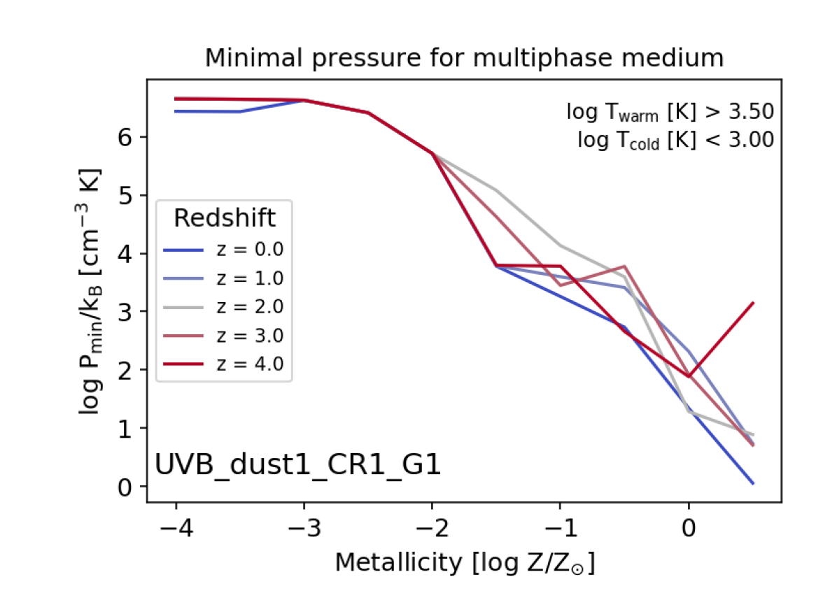
Obrázek 15: Minimum pressure above which a multiphase medium of unshielded and shielded gas in pressure equilibrium, with $\log T_{\mathrm{warm}}[\,\mathrm{K}]>3.5$ and $\log T_{\mathrm{cold}}[\,\mathrm{K}]<3$, is possible in model “UVB_dust1_CR1_G1" for selected redshifts (different line colors). Note that these are the minimum possible pressures for a multiphase medium, based on the thermal equilibrium temperatures (see Figs. 12 and  13). Hydrodynamical simulations are necessary to determine the density (and therefore pressure) distribution of gas along these thermal equilibrium temperature tracks.

5.1 Phase transitions

Ionized - neutral hydrogen:

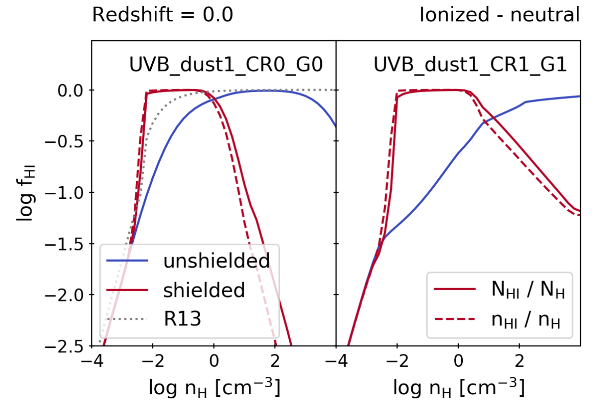
Obrázek 16: Neutral hydrogen fraction for two radiation fields (left panel: only UVB, right panel: UVB + CR + ISRF) along their respective thermal equilibrium temperatures for self-shielded (red lines) and unshielded (blue lines) solar metallicity gas at $z=0$. For self-shielded gas both the volume ($n$) and column ($N$) density H i fractions are shown (solid lines: $N_{\text{H\,{i}}}/N_{\mathrm{H}}$, dashed lines: $n_{\text{H\,{i}}}/n_{\mathrm{H}}$ at the end of the shielding column). The dotted line in the left panel is $f_{\text{H\,{i}}}$ from the fitting function of Rahmati et al. (2013) for the same $T_{\mathrm{eq}}$ as the self-shielded gas.

For each radiation field, the transition from mostly ionized to mostly neutral hydrogen marks where self-shielding becomes important. Assuming that most of the gas follows the thermal equilibrium temperature, the tables directly provide typical hydrogen species fractions for each gas density. Fig. 16 shows $f_{\text{H\,{i}}}$ for solar metallicity and redshift $z=0$ for tables UVB_dust1_CR0_G0 (UVB only, left panel) and UVB_dust1_CR1_G1 (UVB, CRs and ISRF, right panel). For each radiation field, $f_{\text{H\,{i}}}$ is presented for both unshielded (blue) and self-shielded (red) gas. For self-shielded gas, the neutral atomic hydrogen fraction is displayed both as a column density fraction $f_{\text{H\,{i}}}=N_{\text{H\,{i}}}/N_{\mathrm{H}}$ (solid lines) and as a volume density fraction at the end of the shielding column $f_{\text{H\,{i}}}=n_{\text{H\,{i}}}/n_{\mathrm{H}}$ (dashed lines).

For the UVB only tables (UVB_dust1_CR0_G0), we compare $f_{\text{H\,{i}}}$ from this work to the widely used fitting function from R13, for which $n_{\text{H\,{i}}}/n_{\mathrm{H}}$ is a function of gas density, temperature and photoionization rate $\Gamma_{\mathrm{phot}}$. The dotted line in the left panel of Fig. 16 indicates $(n_{\text{H\,{i}}}/n_{\mathrm{H}})_{\mathrm{R13}}$ for the same (equilibrium) temperatures. The characteristic density above which $f_{\text{H\,{i}}}$ for self-shielded gas deviates from unshielded gas is the same in the shielded table and the R13 fitting function. While the transition is very steep in the self-shielded table presented in this work, the fitting function from R13 has a more gradual increase. The difference here may be that $f_{\text{H\,{i}}}$ from the tables assumes that all gas follows the thermal equilibrium temperature and a fixed $n_{\mathrm{H}}-N_{\mathrm{H}}$ relation, while $f_{\text{H\,{i}}}$ from R13 is a fit to cosmological radiative transfer simulations. Note, that in the tables $f_{\text{H\,{i}}}$ can decrease again towards higher densities as hydrogen becomes molecular. Molecular hydrogen is not included in R13.

Atomic - molecular hydrogen:

The transition between atomic and molecular hydrogen is summarised in Fig. 17 for two self-shielded tables (ending with “shield1"). The left panel does not include an interstellar radiation field, while the right panel includes both CRs and the ISRF. In each panel, the H₂ fraction is shown for the thermal equilibrium temperature. The x-axis shows the column density of atomic plus molecular hydrogen through the gas cloud

$$N_{\text{H\,{i}}}+2N_{\mathrm{H2}}=2\times N_{\mathrm{sh}}\cdot\left(\frac{N_{\text{H\,{i}}}}{N_{\mathrm{H}}}+2\frac{N_{\mathrm{H2}}}{N_{\mathrm{H}}}\right)$$ (26)

where $N_{\mathrm{sh}}$ as well as the H i and H₂ fractions are taken from the tables along the thermal equilibrium temperature (hdf5 group /ThermEq/).

For solar metallicity, the results can be compared to observations of H₂ fractions in the Milky Way in sight-lines towards stars (e.g. with Copernicus, Savage et al., 1977) or AGN (e.g. the FUSE halo survey, Gillmon et al., 2006). Inside the Milky Way Galaxy, the transition from atomic to molecular hydrogen (from $\log f_{\mathrm{H2}}\equiv\log 2N_{\mathrm{H2}}/(N_{\text{H\,{i}}}+2N_{\mathrm{H}})\lesssim-3$ to $\log f_{\mathrm{H2}}\gtrsim-1$) has been measured to occur around $\log(N_{\text{H\,{i}}}+2N_{\mathrm{H2}})[\,\mathrm{cm}^{-3}]=20.70$ (Savage et al., 1977), while for high-latitude sight-lines, hydrogen becomes molecular at slightly lower column densities ($\log(N_{\text{H\,{i}}}+2N_{\mathrm{H2}})[\,\mathrm{cm}^{-3}]=20.38$, FUSE halo survey, Gillmon et al., 2006).

Using these tables in hydrodynamical simulations, we find that the gas temperature of individual resolution elements scatters up from the thermal equilibrium temperature but rarely goes below $T_{\mathrm{eq}}$. Higher temperatures for constant density lead to an increase in $N_{\mathrm{ref}}$ and typically to a decrease in $f_{\mathrm{H2}}$. In addition, the tables assume a constant density for each column density, while a sightline in a simulation can go through a variety of gas volume densities. We find that the atomic to molecular transition typically does not scatter to lower column densities in galaxy-scale simulations (Ploeckinger et al. in prep). Therefore, table UVB_dust1_CR1_G1_shield1 matches the column density where the H i-H₂ transition is observed to occur.

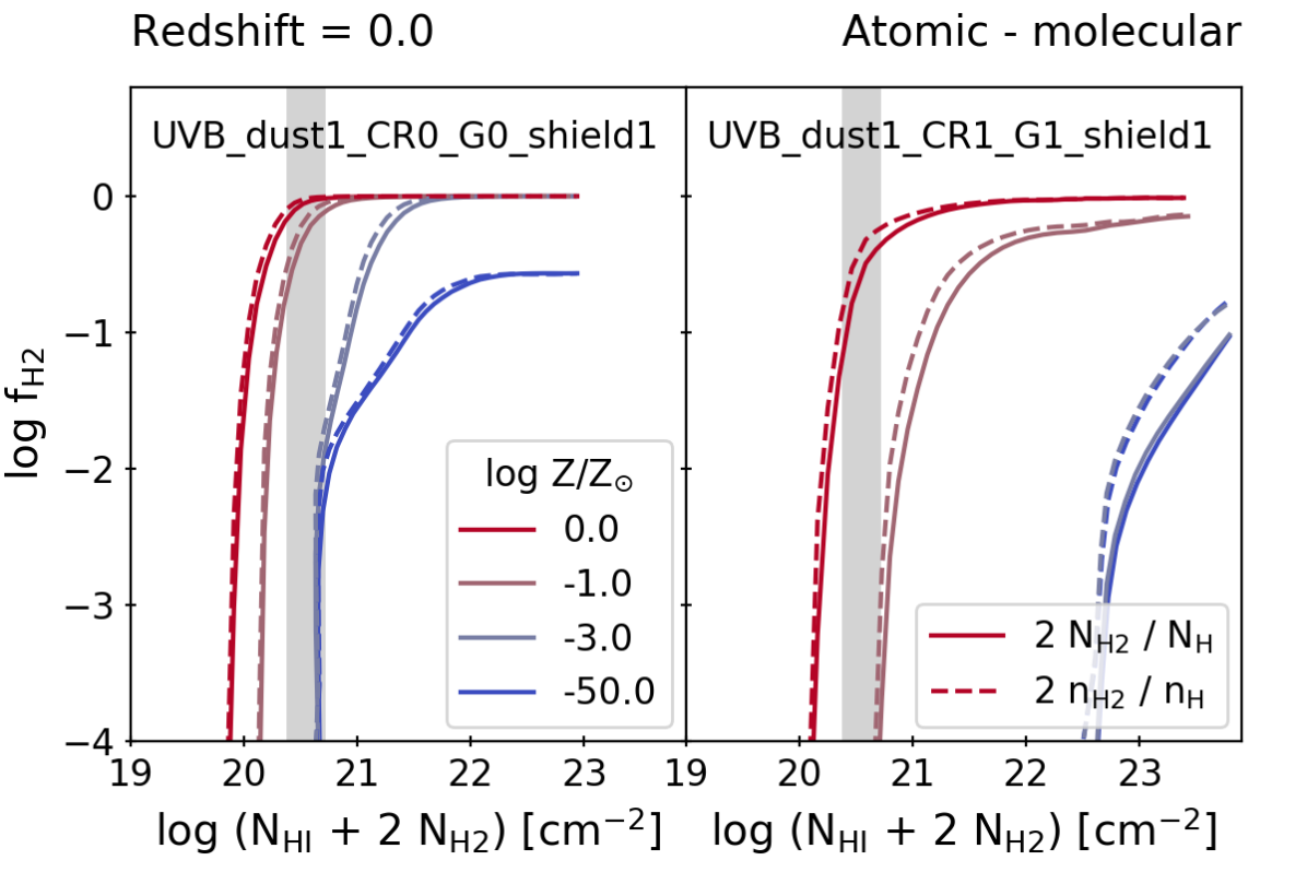
Obrázek 17: Molecular hydrogen fraction $f_{\mathrm{H2}}$, defined as $2N_{\mathrm{H2}}/(N_{\text{H\,{i}}}+2N_{\mathrm{H2}})$ (column density fraction, solid lines) or $2n_{\mathrm{H2}}/(n_{\text{H\,{i}}}+2n_{\mathrm{H2}})$ (volume density fraction at the end of the shielding column, dashed lines) assuming thermal equilibrium temperatures for different radiation fields (different panels) and different metallicities (different line colours) for the self-shielded tables. The grey band brackets the column densities for the observed H i-$\mathrm{H}_{\mathrm{2}}$ transition in the solar neighbourhood, from $\log(N_{\text{H\,{i}}}+2N_{\mathrm{H2}})[\,\mathrm{cm}^{-2}]=20.38$ (FUSE halo survey, Gillmon et al., 2006) to $\log(N_{\text{H\,{i}}}+2N_{\mathrm{H2}})[\,\mathrm{cm}^{-2}]=20.70$ (FUSE disk survey, Gillmon et al., 2006; Copernicus, Savage et al., 1977).

5.2 Ion fractions

Each table contains the gas-phase ion fractions of 11 selected elements (see Table 6). Examples for table UVB_dust1_CR1_G1_shield1 at $z=0$ and for solar metallicity gas in thermal equilibrium are shown for carbon and oxygen (Fig. 18). Ion fractions of all 11 tabulated elements can be found at the project webpages (see Sec. 1 for links).

As hydrogen is the most abundant element and it efficiently absorbs photons with energies higher than 13.6 eV, elements with minimum ionization energies at which the hydrogen photoionization cross section is large (e.g. helium: $E_{i}=24.59\,\mathrm{eV}$, nitrogen: $E_{i}=14.53\,\mathrm{eV}$, oxygen: $E_{i}=13.62\,\mathrm{eV}$, and neon: $E_{i}=21.56\,\mathrm{eV}$), are pre-dominantly neutral in self-shielded gas (see right panel of Fig. 18 for oxygen). Other elements, such as carbon ($E_{i}=11.26\,\mathrm{eV}$) and magnesium ($E_{i}=7.65\,\mathrm{eV}$) are singly ionised over a large range of volume densities (see left panel of Fig. 18 for carbon).

Including dust depletion, the ion volume densities (here illustrated for C ii) can be calculated as

$$n_{\text{C\,{ii}}}=n_{\mathrm{H}}\left(\frac{n_{\text{C\,{ii}}}}{n_{\mathrm{C}}}\right)_{\mathrm{gas}}\left(\frac{n_{\mathrm{C}}}{n_{\mathrm{H}}}\right)_{\mathrm{total}}(1-f_{\mathrm{dust}})\,,$$ (27)

with the gas-phase ion fraction $(n_{\text{C\,{ii}}}/n_{\mathrm{C}})_{\mathrm{gas}}$ (dataset: IonFractions), the dust depletion fraction $f_{\mathrm{dust}}$ (dataset: Depletion), and the element abundance $n_{\mathrm{C}}/n_{\mathrm{H}}$ (dataset: TotalAbundances).

5.3 H2 and CO abundance

Each tables contains the abundances of CO and H₂, both in the last cloudy zone as well as integrated over the full shielding column. Fig. 19 shows these abundances for solar metallicity gas at $z=0$ at its thermal equilibrium temperature for self-shielded tables with and without ISRF and CR rates: UVB_dust1_CR0_G0_shield1 and UVB_dust1_CR1_G1_shield1. While the H2 abundance decreases when the ISRF and CRs are added, at high densities ($\log n_{\mathrm{H}}[\,\mathrm{cm}^{-3}]>4$) the CO abundance is largest when including an ISRF.

A closer look at the molecule abundances is presented in Fig. 20. Here, the dependence of their abundances on the depth into the gas cloud (column density $N_{\mathrm{H}}$) is visualised for the two tables from Fig. 19. For this, an individual grid point (at $\log n_{\mathrm{H}}[\,\mathrm{cm}^{-3}]=4$, see figure caption) is rerun with the additional output for the volume densities of 95 molecule species in each zone. Note that all these molecules are part of the chemistry for all grid points, but this additional output is not stored for the full table. The left panel of Fig. 20 (no ISRF, no CR) explains why gas phase CO is less abundant at the centre of the cloud (here at $N_{\mathrm{H}}\approx 10^{22}\,\,\mathrm{cm}^{-2}$): the majority of CO molecules are condensed into dust grains (“COgrn"). This is also the case for the OH and H₂O molecules (“OHgrn"and “H2Ogrn"). For the stronger radiation field (right panel) molecule fractions peak at much higher column densities and therefore close to the centre of the gas cloud.

The resulting fraction $N_{\mathrm{CO}}/N_{\mathrm{C}}$ for the full shielding column is comparable for both radiation fields at a density of $\log n_{\mathrm{H}}[\,\mathrm{cm}^{-3}]=4$ (see Fig. 19 and triangles in Fig. 20) but without an ISRF, most of the CO is depleted onto dust grains, which explains the reduced gas phase CO fraction for high densities $\log n_{\mathrm{H}}[\,\mathrm{cm}^{-3}]\gtrsim 4$ for the table without the ISRF (UVB_dust1_CR0_G0_shield1).

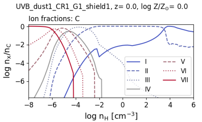
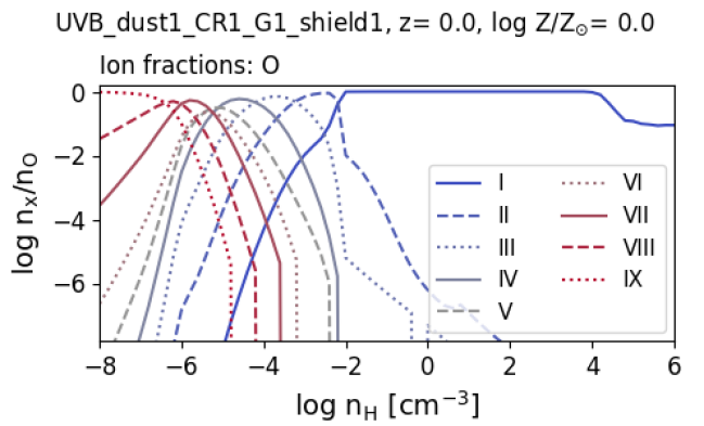
Obrázek 18: Ion fractions at the end of each shielding column for carbon (left) and oxygen (right) for table UVB_dust1_CR1_shield1 at $z=0$ and for solar metallicity assuming thermal equilibrium. For densities of $\log n_{\mathrm{H}}[\,\mathrm{cm}^{-3}]\gtrsim 4.5$ most C and O atoms are in CO. At $\log n_{\mathrm{H}}[\,\mathrm{cm}^{-3}]\approx-2$ the equilibrium temperature decreases steeply with density (compare: red solid line in Fig 12), which explains the features (most noticeable in the C i fraction) around this density.

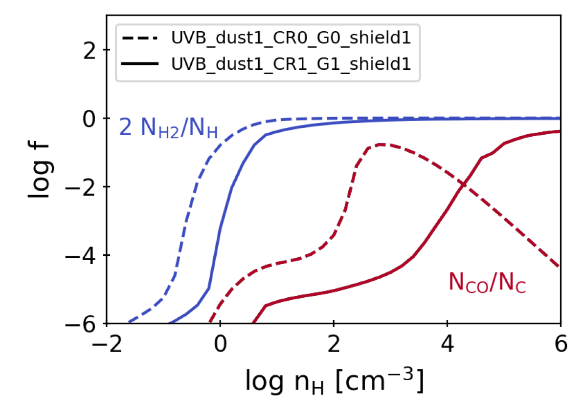
Obrázek 19: CO and H₂ abundances for gas in thermal equilibrium at redshift $z=0$ and solar metallicity. Column density fraction of H2 ($2N_{\mathrm{H2}}/N_{\mathrm{H}}$, blue lines) and CO ($N_{\mathrm{CO}}/N_{\mathrm{C}}$, red lines) for two tables that include self-shielding (no ISRF and no CRs: dashed lines, including ISRF and CR: solid lines). The fraction of CO decreases with density for $\log n_{\mathrm{H}}[\,\mathrm{cm}^{-3}]\gtrsim 3$ for the weaker radiation field (dashed lines) as CO is increasingly depleted onto dust grains (see Fig. 20).

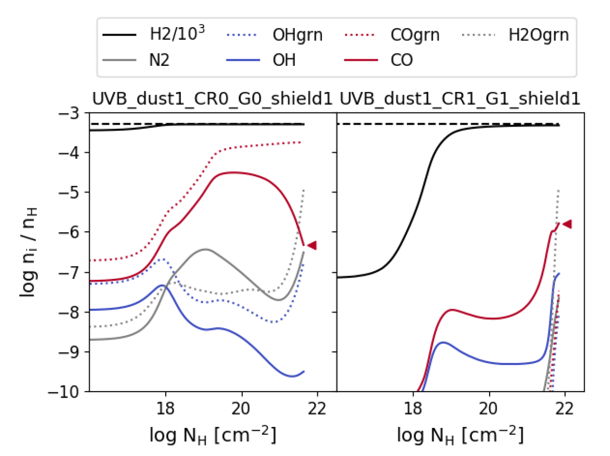
Obrázek 20: Abundances of selected molecules (and their depletion onto dust grains, indicated by the suffix “grn") along the shielding column at an individual grid point of two tables (left panel: UVB_dust1_CR0_G0_shield1, right panel: UVB_dust1_CR1_G1_shield1) for the respective equilibrium temperatures at the end of the shielding columns ($\log T[K]=1.00$, left and 1.41, right) of $z=0$, solar metallicity gas with a volume density of $\log n_{\mathrm{H}}[\,\mathrm{cm}^{-3}]=4$. The H₂ abundance $n_{\mathrm{H2}}/n_{\mathrm{H}}$, has been reduced by a factor of $10^{3}$ to fit on the plot. For guidance, the horizontal dashed line indicates the abundance where all H is in H₂. As seen in Fig. 19, the CO abundance at the last zone (indicated by a red triangle) for this density is comparable for both radiation fields, but the distribution throughout the column is very different.

6 Example results: Emission lines

Out of the 183 emission lines listed in Table 7 we show a few examples of soft X-ray emission lines in Fig. 21 and far-infrared/(sub-)mm emission lines in Fig. 22. In both figures the normalized emergent emissivities, $\epsilon/n_{\mathrm{H}}^{2}$, for the last cloudy zone of the shielding column ($\epsilon_{\mathrm{Vol}}$) as well as the emissivity calculated by dividing the line intensity of the full shielding column by the length of the shielding column ($\epsilon_{\mathrm{Col}}$) from the fiducial model “UVB_dust1_CR1_G1_shield1" are displayed.

Fig. 21 shows the strongest soft X-ray emission lines of O vii and O viii (as in the top panels of figure 1 in Bertone et al., 2010). For densities $\log n_{\mathrm{H}}[\,\mathrm{cm}^{-3}]\gtrsim-3$ (see left panel for $\log n_{\mathrm{H}}[\,\mathrm{cm}^{-3}]=0$) the emissivities $\epsilon_{\mathrm{Vol}}$ (solid lines) and $\epsilon_{\mathrm{Col}}$ (dotted lines) agree, as expected for unshielded gas. For very low densities (e.g. $\log n_{\mathrm{H}}[\,\mathrm{cm}^{-3}]=-6$, right panel) $\epsilon_{\mathrm{Vol}}$ and $\epsilon_{\mathrm{Col}}$ disagree for photo-ionized gas ($\log T[\,\mathrm{K}]\lesssim 6$). This has been traced down to differences between the output produced by the cloudy commands “save lines emissivity" and “save line list absolute" and even persists for one-zone models (e.g. “UVB_dust1_CR1_G1_shield0"). The unexpected behaviour of cloudy has been posted to the cloudy group (see https://cloudyastrophysics.groups.io/g/Main/message/4301 for details). This is unlikely affecting any simulation results as this issue only appears at very low densities where the emissivities are very small.

The results for selected CO lines as well as the C ii emission line at $157\,\mu\mathrm{m}$ are presented in Fig. 22 for densities of $\log n_{\mathrm{H}}[\,\mathrm{cm}^{-3}]=2$ (left panel) and $\log n_{\mathrm{H}}[\,\mathrm{cm}^{-3}]=4$ (right panel). For higher densities the CO fraction increases and therefore the normalized emissivity of C ii decreases. At $\log n_{\mathrm{H}}[\,\mathrm{cm}^{-3}]=4$ (right panel) CO is collisionally excited to higher energy levels, leading to brighter emission lines of higher level transitions (compare e.g. $J=1\rightarrow 0$ at 2600 $\mu\mathrm{m}$ and $J=3\rightarrow 2$ at 867 $\mu\mathrm{m}$).

As CO forms mainly deep into the shielding column (see e.g. right panel of Fig. 20), the emissivities calculated at the last zone ($\epsilon_{\mathrm{Vol}}$, solid lines) are not expected to be identical to the shielding column averaged emissivity ($\epsilon_{\mathrm{Col}}$, dotted lines) but they converge to the same values for temperatures $\log T[\mathrm{K}]\gtrsim 4$, where the shielding column becomes small.

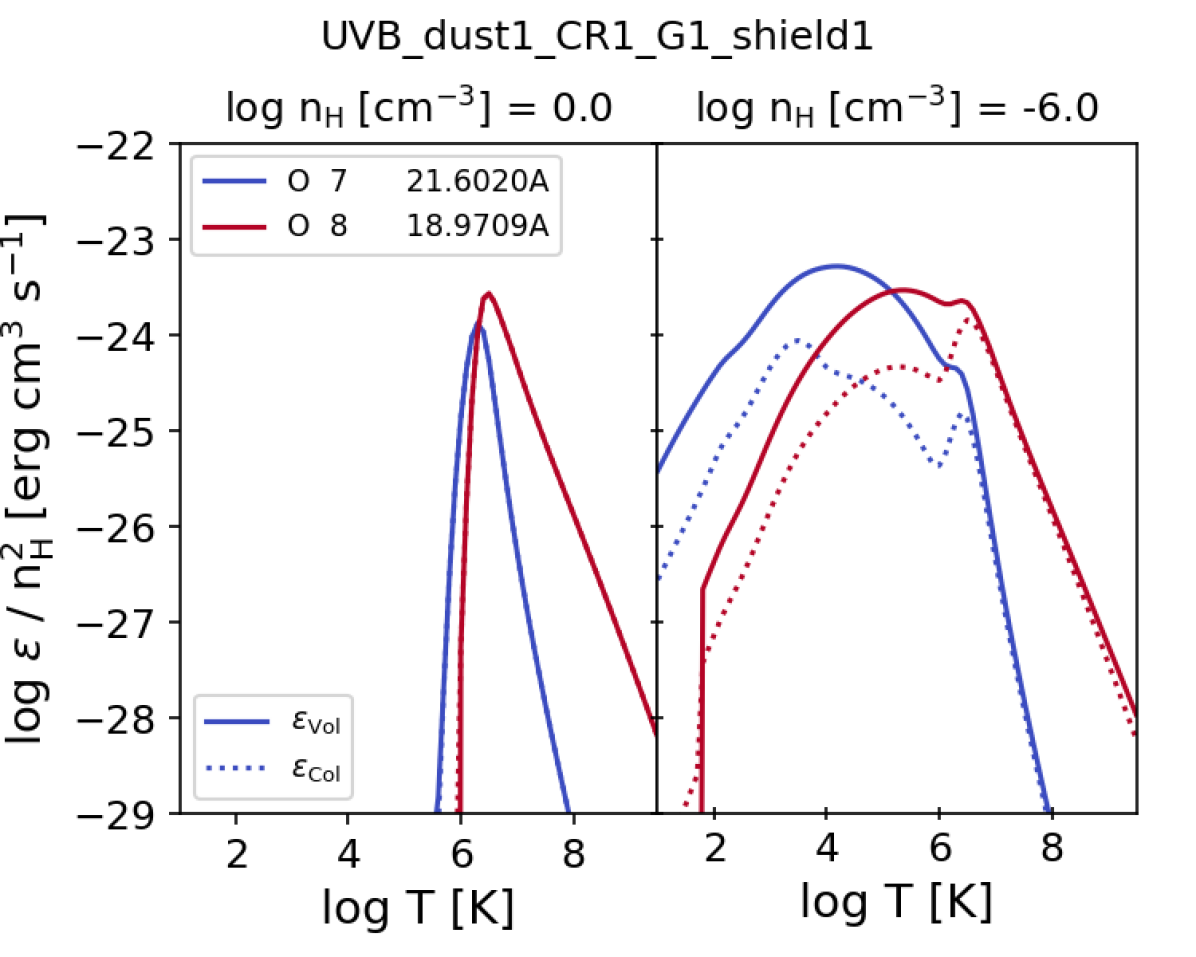
Obrázek 21: The normalized emergent emissivities, $\epsilon/n_{\mathrm{H}}^{2}\,[\mathrm{erg}\,\mathrm{cm}^{3}\,s^{-1}]$ for selected soft X-ray emission lines for constant hydrogen number density (left panel: $\log n_{\mathrm{H}}[\,\mathrm{cm}^{-3}]=0$, right panel: $\log n_{\mathrm{H}}[\,\mathrm{cm}^{-3}]=-6$), solar metallicity and redshift $z=0$. The solid lines are the emissivities at the last cloudy zone ($\epsilon_{\mathrm{Vol}}$, dataset: EmissivitiesVol) and the dotted lines are the average emissivities of the full shielding column ($\epsilon_{\mathrm{Col}}$, dataset: EmissivitiesCol). For diffuse gas (right panel) with temperatures below $\log T[\,\mathrm{K}]\lesssim 6$, photo-ionization dominates over collisional ionization and the line emissivity therefore depends on density (compare different panels). The differences between $\epsilon_{\mathrm{Vol}}$ and $\epsilon_{\mathrm{Col}}$ for $\log n_{\mathrm{H}}[\,\mathrm{cm}^{-3}]=-6$ (right panel) are unexpected as the gas is unshielded at this density and the variations within the small shielding column are negligible. This is likely an artefact in cloudy (see text for details).

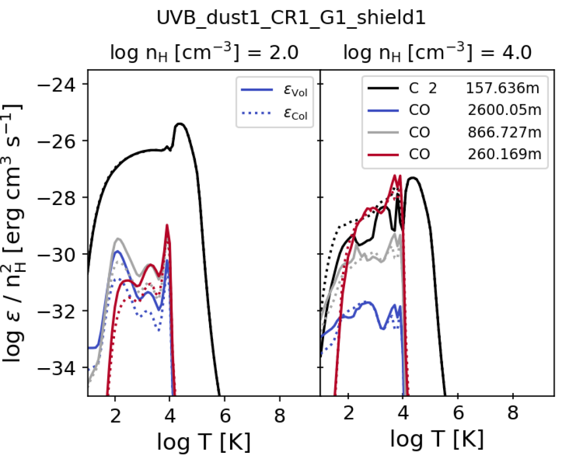
Obrázek 22: As Fig. 21 but for selected (sub-)mm / far infrared emission lines for high density gas (left panel: $\log n_{\mathrm{H}}[\,\mathrm{cm}^{-3}]=2$, right panel: $\log n_{\mathrm{H}}[\,\mathrm{cm}^{-3}]=4$). As molecules form in self-shielded gas and their abundance and level population depend on the shielding column density, the emissivity at the last cloudy zone $\epsilon_{\mathrm{Vol}}$ (i.e. the most shielded part of the gas column, solid lines) of the selected CO lines is typically larger than the average line emissivity of the shielding column $\epsilon_{\mathrm{Col}}$ (dotted lines). For high densities (e.g. $\log n_{\mathrm{H}}[\,\mathrm{cm}^{-3}]=4$, right panel) the emissivity of C ii (“C 2") is lower at high shielding column densities and therefore the column averaged emissivity is larger than the emissivity at the last cloudy zone ($\epsilon_{\mathrm{Col}}>\epsilon_{\mathrm{Vol}}$).

7 Summary

We use cloudy version 17.01 to tabulate the properties of unshielded and self-shielded gas as it is exposed to metagalactic and interstellar radiation fields. The tables cover a sufficiently large range in redshift ($z=0$ - $9$), temperature ($\log T[K]=1$ - $9.5$), metallicity ($\log Z/\mathrm{Z}_{\odot}=-4$ - $+0.5$, $Z=0$), and density ($\log n_{\mathrm{H}}[\,\mathrm{cm}^{-3}]=-8$ - $+6$) to enable users to use one set of tables for all gas phases (ionised, atomic, molecular) both during a simulation (i.e. cooling and heating rates) as well as for analysing the simulation output in post-processing (i.e. species fractions, line emissivities).

The gas column density is an important factor to estimate both the local star formation rate as well as the attenuation of the radiation field. The reference column density $N_{\mathrm{ref}}$ in this work is based on the Jeans column density $N_{\mathrm{J}}$, which is a typical scale for self-gravitating gas. As gas surface density is observed to correlate with the star formation rate surface density (Eq. 10), we add an interstellar radiation field (ISRF) and cosmic rays proportional to $N_{\mathrm{ref}}^{1.4}$ to the redshift-dependent UV/X-ray background. The UV (and X-ray) background is based on the model from FG20 but before hydrogen and helium reionization are complete, we attenuate the FG20 spectra to better match the effective rates inferred from observations by FG20 and therefore the observed electron scattering optical depth of $\tau_{e}=0.054$ (Planck Collaboration et al., 2018).

Dust grains are an important catalyst for the formation of $\mathrm{H}_{\mathrm{2}}$ and other molecules and also contribute to self-shielding. A constant dust-to-metals ratio is assumed for star formation rate surface densities above the solar neighbourhood value, while for lower $N_{\mathrm{ref}}$, the dust-to-metal ratio scales like the ISRF ($\propto N_{\mathrm{ref}}^{1.4}$, Eq. 18). The gas phase abundances of individual metals that are depleted onto dust grains are reduced accordingly.

At the centre of a gas cloud, the radiation field is attenuated by gas with a shielding column of $N_{\mathrm{sh}}=0.5N_{\mathrm{ref}}$ and the dust within. This is modelled by passing the incident radiation field through a gas shielding column, $N_{\mathrm{sh}}$. A large number of gas properties (see Table 6 for a full list) is stored in hdf5 datasets at the unattenuated (unshielded; tables with _shield0) edge of the gas clump, as well as at the gas cloud centre (self-shielded; tables with _shield1). Selected properties (e.g CO and H species fractions, line emissivities) are also available as averages over the shielding column. In the tables for self-shielded gas, all elements (also all metals) contribute to the self-shielding and in turn respond to the attenuated radiation field. Some datasets (e.g. cooling and heating rates in Figs. 11 and 9, ion fractions in Figs. 18) are presented for individual slices through the multi-dimensional hyper cuboid and we provide an easy to use graphical user interface to explore the full range.

As an example application, we showed characteristic densities for the most important phase transitions ($\mathrm{H}_{\mathrm{2}}$ to H i, Fig. 16, and H i to H ii, Fig. 17) and compared the results to values from the literature. For the transition from ionised to neutral hydrogen, we compared our results to the fitting function from R13. Fig. 16 illustrates that self-shielding becomes important at very similar densities, although the increase in $f_{\text{H\,{i}}}$ with density is steeper in this work than in R13.

The predicted transition between neutral and molecular hydrogen was compared to observations of individual sight lines within the MW disk and towards the MW halo, measuring both the H i and $\mathrm{H}_{\mathrm{2}}$ column densities (Fig. 17). For our fiducial ISRF and CR rates (UVB_dust1_CR1_G1_shield1) the observations are very well matched.

Two tables (UVB_dust1_CR1_G1_shield0 and UVB_dust1_CR1_G1_shield1) include line emissivities for 183 selected lines. A full overview of the data files released with this work is in Table 8. In addition to the hdf5 data files we also provide a set of C routines that interpolate the tables and return the total net cooling rate for a given redshift, gas density, temperature, and metallicity or abundance ratio, which can be implemented in a hydrodynamics code, and a set of python3 routines that read the tables and produce plots via an easy to use graphical user interface. All data files and links to the github repositories for the python and C packages can be found at http://radcool.strw.leidenuniv.nl/ and https://www.sylviaploeckinger.com/radcool.

Finally, practical information about how to use the tables in simulations, either alone or coupled to a non-equilibrium network, such as chimes (Richings et al., 2014a, b) or grackle (Smith et al., 2017), as well as how to reproduce our results with the public code cloudyv17.01 are provided in the appendix.

Tabulka 8: Summary of files released with this work at http://radcool.strw.leidenuniv.nl/ and https://www.sylviaploeckinger.com/radcool.

File name	Description
$<$modelname$>$.hdf5	Hdf5 files with cooling and heating rates, ion fractions, free electron fractions and molecule abundances for each model listed in Table 5. The content of each datafile is listed in Table 6 and described in Sec. 4.1.
$<$modelname$>$_lines.hdf5	Hd5 files for models UVB_dust1_CR1_G1_shield0 and UVB_dust1_CR1_G1_shield1 containing the emissivities for the emission lines listed in Table 7 and described in Sec. 4.2.
modFG20_cloudy.ascii	The modified FG20 spectra in the cloudy UVB format. See Appendix C for how to use this UVB with cloudy.

Tabulka 9: Overview of the cooling processes stored in the hdf5 tables, with their index in the cooling datasets (column 1), their string identifiers (column 2), and their scaling (column 3, see text for details). Column 4 lists the cloudy labels for the individual cooling channels and additional information can be found in column 5. The star in column 1 indicates processes that are combined in “TotalPrim" while the remaining ones are combined in “TotalMetal".

i	Identifier	Scaling	cloudy label	Comment
0$\star$	Hydrogen	$n_{\mathrm{H}}$	H, H-fb	H-fb: H + e $\rightarrow$ H- + h$\nu$
1$\star$	Helium	$n_{\mathrm{He}}$	He
2	Carbon	$n_{\mathrm{C}}$	C
3	Nitrogen	$n_{\mathrm{N}}$	N
4	Oxygen	$n_{\mathrm{O}}$	O
5	Neon	$n_{\mathrm{Ne}}$	Ne
6	Magnesium	$n_{\mathrm{Mg}}$	Mg
7	Silicon	$n_{\mathrm{Si}}$	Si
8	Sulphur	$n_{\mathrm{S}}$	S
9	Calcium	$n_{\mathrm{Ca}}$	Ca
10	Iron	$n_{\mathrm{Fe}}$	Fe
11	OtherA	Z	Li, Be, B, F, Na, Al,	all other atoms
			P, Cl, Ar, K, Sc, Ti, V,
			Cr, Mn, Co, Ni, Cu, Zn
12$\star$	H2	$n_{\mathrm{H2}}$	H2cX	H2 cooling from: collisions,
			H2ln, H2+	H2 lines, photo continuum cooling
13	molecules	Z	molecule	cooling from all molecules other than H2 and HD
14$\star$	HD	$n_{\mathrm{HD}}$	HD	HD rotation cooling (see Sec. 2.5 for details)
15$\star$	NetFFH		FFcm_H	net free-free brems cooling from H and He ions
16	NetFFM	Z	FFcm_M	net free-free brems cooling from metal ions
17$\star$	eeBrems	$n_{\mathrm{e}}^{2}$	eeff	electron - electron bremsstrahlung
18$\star$	Compton		Compton	Compton cooling
19	Dust	Z	dust	dust cooling
20$\star$	TotalPrim	prim		0, 1, 12, 14, 15, 17, 18
21	TotalMetal	metal		2, 3, 4, 5, 6, 7, 8, 9, 10, 11, 13, 16, 19

Tabulka 10: As Table 9 but for the individual heating contributions.

ID Heat	Identifier	Scaling	cloudy label	Comment
0$\star$	Hydrogen	$n_{\mathrm{H}}$	H, H-,	H- heating,
			Hn=2	Hn=2: net hydrogen photoionization heating of all excited states
1$\star$	Helium	$n_{\mathrm{He}}$	He, He3l	He3l: helium triplet line heating
2	Carbon	$n_{\mathrm{C}}$	C
3	Nitrogen	$n_{\mathrm{N}}$	N
4	Oxygen	$n_{\mathrm{O}}$	O
5	Neon	$n_{\mathrm{Ne}}$	Ne
6	Magnesium	$n_{\mathrm{Mg}}$	Mg
7	Silicon	$n_{\mathrm{Si}}$	Si
8	Sulphur	$n_{\mathrm{S}}$	S
9	Calcium	$n_{\mathrm{Ca}}$	Ca
10	Iron	$n_{\mathrm{Fe}}$	Fe, Fe 2	Fe 2 line heating
11	OtherA	Z	Li, Be, B, F, Na, Al,	all other atoms
			P, Cl, Ar, K, Sc, Ti, V,
			Cr, Mn, Co, Ni, Cu, Zn
12$\star$	H2	$n_{\mathrm{H2}}$	H2vH	H2 heating from: collisions,
			H2dH, H2+	photodissociation, H2+ heating
			H2ph	photoionization heating
13	COdiss	$n_{\mathrm{CO}}$	COds	CO dissociation heating
14$\star$	CosmicRay	CR rate	CR H	cosmic ray heating
15	UTA	Z	UTA	unresolved transition array (UTA) heating
16	line	Z	line	heating due to induced line absorption of continuum
17$\star$	Hlin		Hlin	iso-sequence line heating
18	ChaT	Z	ChaT	heating due to charge transfer:
				- ionization of heavy element, recombination of hydrogen
				- recombination of heavy element, ionization of hydrogen)
19$\star$	HFF		H FF	free-free heating (if Bremsstrahlung has a net heating effect)
20$\star$	Compton		Compton	Compton heating
21	Dust	Z	GrnP, GrnC	grain photoionization, grain collisions
22$\star$	TotalPrim	prim		0, 1, 12, 14, 17, 19, 20
23	TotalMetal	Z		2, 3, 4, 5, 6, 7, 8, 9, 10, 11, 13, 15, 16, 17, 18, 21

Data availability

The data underlying this article are available in the Harvard Dataverse, at https://dataverse.harvard.edu/dataverse/radcool (rates and fractions data files: https://doi.org/10.7910/DVN/GR3L5N, line emissivities data files: https://doi.org/10.7910/DVN/CRJ7GT). More information as well as the routines to use and visualise the tables can be found at http://radcool.strw.leidenuniv.nl/ and https://www.sylviaploeckinger.com/radcool.

Příloha A How to use the tables

The tables released with this work cover a large range of redshifts, temperatures, metallicities and densities. For any dataset listed in Table 6, its value can be obtained at any point in this multi-dimensional space by a 4D interpolation. Due to the relatively fine spacing, the exact interpolation scheme or whether different weights are applied for different dimensions, is unimportant. We recommend a linear interpolation in log and weighting the different dimensions equally, but other interpolation schemes are possible. An interpolation in log space can lead to species fractions not summing up to 1, even if the fractions at the individual grid points do. In this case, the fractions can be re-normalised to 1 after the interpolation.

For solar abundance ratios the total cooling rate $\Lambda_{\mathrm{cool,total}}$ is

$$\Lambda_{\mathrm{cool,total}}(z,T,Z,n_{\mathrm{H}})= \Lambda_{\mathrm{cool,TotalPrim}}(z,T,Z,n_{\mathrm{H}})$$ (28)

$$+ \Lambda_{\mathrm{cool,TotalMetal}}(z,T,Z,n_{\mathrm{H}})$$

but in the more general case, where the abundance ratios differ from the solar values, the total cooling rate is calculated as

$$\Lambda_{\mathrm{cool,total}}(z,T,Z,n_{\mathrm{H}})= \sum_{i}\frac{(n_{i}/n_{\mathrm{H}})}{(n_{i}/n_{\mathrm{H}})_{\mathrm{table}}}\Lambda_{\mathrm{cool,i}}(z,T,Z,n_{\mathrm{H}})$$ (29)

$$+\Lambda_{\mathrm{cool,OtherA}}(z,T,Z,n_{\mathrm{H}})$$

$$+\Lambda_{\mathrm{cool,H2}}(z,T,Z,n_{\mathrm{H}})$$

$$+\Lambda_{\mathrm{cool,molecules}}(z,T,Z,n_{\mathrm{H}})$$

$$+\Lambda_{\mathrm{cool,HD}}(z,T,Z,n_{\mathrm{H}})$$

$$+\Lambda_{\mathrm{cool,NetFFH}}(z,T,Z,n_{\mathrm{H}})$$

$$+\Lambda_{\mathrm{cool,NetFFM}}(z,T,Z,n_{\mathrm{H}})$$

$$+\Lambda_{\mathrm{cool,eeBrems}}(z,T,Z,n_{\mathrm{H}})$$

$$+\Lambda_{\mathrm{cool,Compton}}(z,T,Z,n_{\mathrm{H}})$$

$$+\Lambda_{\mathrm{cool,Dust}}(z,T,Z,n_{\mathrm{H}})$$

where $i$ loops over all individually traced elements (see Table 3). Analogously, the total heating rate $\Lambda_{\mathrm{heat,total}}$ can be calculated by summing up either only the components $\Lambda_{\mathrm{heat,TotalPrim}}$ and $\Lambda_{\mathrm{heat,TotalMetal}}$ (for solar abundances) or the full list of heating channels (Table 10) for general abundance ratios.

In Sec. A.1 we discuss how the cooling and heating rates can also be calculated for values outside the table ranges. In addition, Sec. A.2 demonstrates how the tables can be combined with a reduced non-equilibrium network.

A.1 Extrapolation outside the table boundaries

Redshift

The redshift dimension in the tables goes from $z_{\mathrm{min}}=0$ to $z_{\mathrm{max}}=9$ . For redshifts larger than $z_{\mathrm{max}}$, the Compton cooling should not be used from the tables as it is highly redshift dependent. Instead, the change in cooling rate due to inverse Compton cooling off the CMB can be calculated analytically with (e.g. Mo et al., 2010):

$$\Lambda_{\mathrm{cool,Compton}}/n_{\mathrm{H}}^{2}= \frac{4k_{\mathrm{B}}}{m_{\mathrm{e}}c}\,\sigma_{\mathrm{T}}\,\frac{n_{\mathrm{e}}}{n_{\mathrm{H}}^{2}}\,a\,\left[T_{\mathrm{CMB,0}}(1+z)\right]^{4}\cdot$$ (30)

$$[T-T_{\mathrm{CMB,0}}(1+z)]\quad\mathrm{erg\,cm^{3}\,s^{-1}}$$ (31)

with the Boltzmann constant $k_{\mathrm{B}}=1.38066\times 10^{-16}\,\mathrm{cm}^{2}\mathrm{g}\,\mathrm{s}^{-2}\,\mathrm{K}^{-1}$, the electron mass $m_{\mathrm{e}}=9.11\times 10^{-28}\,\mathrm{g}$, the speed of light $c=2.998\times 10^{10}\,\mathrm{cm}\,\mathrm{s}^{-1}$, the Thomson cross-section $\sigma_{\mathrm{T}}=6.65\times 10^{-25}\,\mathrm{cm}^{2}$, the radiation constant $a=7.57\times 10^{-15}\,\mathrm{erg\,cm^{-3}\,K^{4}}$, the present day CMB temperature $T_{\mathrm{CMB,0}}=2.73\,\mathrm{K}$, the electron number density $n_{\mathrm{e}}$, the hydrogen number density $n_{\mathrm{H}}$, the gas temperature $T$, and the current redshift $z$. The electron density $n_{\mathrm{e}}$ can be taken from the redshift bin $z=z_{\mathrm{max}}$ for $z>z_{\mathrm{max}}$.

Temperature

We impose a minimum temperature of $10\,\,\mathrm{K}$ and advise to impose a similar temperature floor in all simulations that make use of this tables. In case the temperature exceeds the maximum temperature $T_{\mathrm{max}}=10^{9.5}\,\,\mathrm{K}$, the contributions from “eeBrems", “NetFFH", and “Compton” cooling processes can be linearly extrapolated using the slope between $\log T[\,\mathrm{K}]=9$ and $\log T[\,\mathrm{K}]=9.5$ for $\log\Lambda_{\mathrm{cool,i}}(T)$ with $i$ is “eeBrems", “NetFFH", and “Compton”. The sum of these three extrapolations is the total cooling rate. All other cooling contributions, as well as all heating processes that we compute are negligible for $T>T_{\mathrm{max}}$.

Metallicity

For all heating and cooling processes $i$ that scale with either an element abundance or with metallicity (as indicated in Tables 9 and 10), the cooling (heating) rate for metallicities above the maximum metallicity of $Z_{\mathrm{max}}=10^{0.5}{\mathrm{Z}}_{\odot}$ can be approximated by

$$\Lambda_{\mathrm{cool,i}}=\frac{Z}{Z_{\mathrm{max}}}\Lambda_{\mathrm{cool,i,Zmax}}$$ (32)

$$\Lambda_{\mathrm{heat,i}}=\frac{Z}{Z_{\mathrm{max}}}\Lambda_{\mathrm{heat,i,Zmax}}$$ (33)

for metallicity scaling and

$$\Lambda_{\mathrm{cool,i}}=\frac{n_{\mathrm{x}}/n_{\mathrm{H}}}{(n_{\mathrm{x}}/n_{\mathrm{H}})_{\mathrm{max}}}\Lambda_{\mathrm{cool,i,Zmax}}$$ (34)

$$\Lambda_{\mathrm{heat,i}}=\frac{n_{\mathrm{x}}/n_{\mathrm{H}}}{(n_{\mathrm{x}}/n_{\mathrm{H}})_{\mathrm{max}}}\Lambda_{\mathrm{heat,i,Zmax}}$$ (35)

for element abundance scaling. Here $\Lambda_{\mathrm{cool,i,Zmax}}$ and $\Lambda_{\mathrm{heat,i,Zmax}}$ are the cooling and heating rates for the highest tabulated metallicity bin for the considered redshift, density, and temperature. $(n_{\mathrm{x}}/n_{\mathrm{H}})_{\mathrm{max}}$ is the maximum abundance of element $x$.

Cooling or heating channels labelled with $\star$ (primordial) in Tables 9 and 10 do not scale with metallicity and should therefore be approximated by the maximum metallicity table entry:

$$\Lambda_{\mathrm{cool,i}}=\Lambda_{\mathrm{cool,i,Zmax}}$$ (36)

$$\Lambda_{\mathrm{heat,i}}=\Lambda_{\mathrm{heat,i,Zmax}}$$ (37)

neglecting the shielding from additional metals.

The metallicity bins are spaced logarithmically with an additional metallicity bin for primordial abundances and therefore $Z=0$. The primordial abundances can be used for $Z<Z_{\mathrm{min}}$, where $Z<Z_{\mathrm{min}}$ is the minimum (for $Z\neq 0$) metallicity in the tables ($\log(Z/{\mathrm{Z}}_{\odot})_{\mathrm{min}}=-4$).

Density

At high densities, where collisional ionization dominates over photo-ionization, most cooling rates scale as $n_{\mathrm{H}}n_{\mathrm{e}}$ while most heating rates scale with $n_{\mathrm{H}}$. For convenience, cooling and heating rates are both stored as $\left[\Lambda_{\mathrm{cool}}/n_{\mathrm{H}}^{2}\right]$ and $\left[\Lambda_{\mathrm{heat}}/n_{\mathrm{H}}^{2}\right]$, respectively. Assuming a constant free electron fraction for $n_{\mathrm{H}}\geq n_{\mathrm{H,max}}$, the cooling and heating rates can be extrapolated as

$$\Lambda_{\mathrm{cool}}(n_{\mathrm{H}}>n_{\mathrm{H,max}})=\left[\frac{\Lambda_{\mathrm{cool}}}{n_{\mathrm{H,max}}^{2}}\right]\,n_{\mathrm{H}}^{2}$$ (38)

and

$$\Lambda_{\mathrm{heat}}(n_{\mathrm{H}}>n_{\mathrm{H,max}})=\left[\frac{\Lambda_{\mathrm{heat}}}{n_{\mathrm{H,max}}^{2}}\right]\,n_{\mathrm{H}}\,n_{\mathrm{H,max}}\;.$$ (39)

A.2 Coupling with a reduced non-equilibrium network

If the timescales for ionization and recombination are long compared to the dynamical timescale or the cooling / heating timescale, local ionization equilibrium is not a good assumption. As the number of species and reactions increase steeply with the number of elements, it is computationally very expensive to run a non-equilibrium network for a large number of elements.

The smallest networks only calculate hydrogen and helium in non-equilibrium and add metal cooling from look-up tables. Other networks include more species and reactions to also trace the formation of CO. Independently of the elements included in a network, it can easily be combined with the tables presented in this work.

Cooling / heating rates:

The cooling and heating rates are tabulated according to the individual processes, as listed in Tables 9 and 10. If the (net) cooling rates for e.g. hydrogen and helium are calculated from the network, then any remaining cooling channels that are not included in the network can be obtained from the tables and added.

Electron densities:

The total number density of free electrons can be obtained in a similar way as explained above for the total cooling / heating rates. The dataset ElectronFractions contains the fraction of free electrons per hydrogen nucleus ($n_{\mathrm{e}}/n_{\mathrm{H}}$) split into the contributions from each element. This allows one to individually add the electron density from each element that is not included in the network.

Cooling processes typically include an interaction between an electron and another species, for example a carbon atom (i.e. collisional excitation, collisional ionization, recombination cooling, free-free emission), and scale therefore generally as $\Lambda_{\mathrm{cool}}\propto n_{\mathrm{e}}n_{\mathrm{H}}$ (if each species number density scales with the hydrogen number density). As we tabulate the electron densities individually for each element, a non-equilibrium network can scale the metal cooling rates by the combined free electron density $n_{\mathrm{e,comb}}=(n_{\mathrm{e,H}}+n_{\mathrm{e,He}})_{\mathrm{neq}}+(n_{\mathrm{e}})_{\mathrm{eq}}$. In this example, the free electrons from hydrogen ($n_{\mathrm{e,H}}$) and helium ($n_{\mathrm{e,He}}$) are taken from the non-equilibrium (“neq") calculations while the free electrons from metals ($n_{\mathrm{e}}$) are added from the equilibrium (“eq") tables from this work.

If the metal cooling rates are scaled as $\Lambda_{\mathrm{comb}}=\Lambda_{\mathrm{table}}(n_{\mathrm{e,comb}}/n_{\mathrm{e,table}})$ the cooling rates $\Lambda_{\mathrm{comb}}$, while calculated assuming ionization equilibrium (as in $\Lambda_{\mathrm{table}}$), capture many of the non-equilibrium effects for metal cooling. For the heating rates this additional scaling is not necessary as $\Lambda_{\mathrm{heat}}$ scales with $n_{\mathrm{H}}$.

Příloha B Including the effective FG20 background radiation field

Before and during reionization, the photo-ionization rates calculated from the redshift-dependent UV / X-ray spectra from FG20 differ from their tabulated “effective" photo-ionization rates that are modelled to match the observed electron scattering optical depth of $\tau_{e}=0.054$ (Planck Collaboration et al., 2018). As cloudy uses a full spectrum as input radiation field, we modify the spectra from FG20 to match their “effective" photo-ionization rates. Assuming that before H i reionization, the H i ionizing radiation is attenuated by neutral hydrogen gas with a column density $N_{\text{H\,{i}}}$ (and before He ii reionization, the He ii ionizing radiation is attenuated by singly ionized helium gas with column density $N_{\text{He\,{ii}}}$), the new spectrum $J_{\nu}^{\mathrm{modFG20}}$ can be derived from the original FG20 spectrum $J_{\nu}^{\mathrm{FG20}}$ as

$$J_{\nu}^{\mathrm{modFG20}}=J_{\nu}^{\mathrm{FG20}}\,e^{-\sigma_{\text{H\,{i}}}(\nu)N_{\text{H\,{i}}}}\,e^{-\sigma_{\text{He\,{ii}}}(\nu)N_{\text{He\,{ii}}}}$$ (40)

The photo-ionization cross sections $\sigma_{\text{H\,{i}}}$ and $\sigma_{\text{He\,{ii}}}$ are taken from Verner et al. (1996) and the column densities $N_{\text{H\,{i}}}$ and $N_{\text{He\,{ii}}}$ are free parameters that can be chosen so that the photo-ionization rates calculated from $J_{\nu}^{\mathrm{modFG20}}$ are equal to the effective rates from FG20. The effective He ii photo-ionization from FG20 decreases very steeply for $z>4$ which would lead to arbitrarily high column densities. We therefore use a maximum shielding column of $N_{\text{H\,{i}}\mathrm{,max}}=10^{20}\,\mathrm{cm}^{-2}$ and $N_{\text{He\,{ii}}\mathrm{,max}}=(n_{\mathrm{He}}/n_{\mathrm{H}})_{\mathrm{prim}}\times N_{\text{H\,{i}}\mathrm{,max}}$, where $(n_{\mathrm{He}}/n_{\mathrm{H}})_{\mathrm{prim}}=0.08246$ is the primoridal helium abundance, yielding a non-zero photo-ionization rate of He ii between $z=4$ and $z=8$ (see Fig. 24).

Fig. 23 displays $J_{\nu}^{\mathrm{modFG20}}$ (black solid lines) used in this work and $J_{\nu}^{\mathrm{FG20}}$ (red dashed lines) for four different redshifts. The top panels show the spectrum after (left, $z=3.0$) and during (right, $z=3.5$) He ii reionization and the bottom panels illustrate the UVB spectrum after (left, $z=7.2$) and during (right, $z=7.8$) H i reionization. For $z\leq 3$ ($z_{\mathrm{rei},\text{He\,{ii}}}-\Delta z_{\mathrm{rei},\text{He\,{ii}}}=3$), both spectra are identical, as the FG20 effective rates match the rates from the spectra in FG20 and no additional attenuation is necessary.

The photo-ionization and photo-heating rates calculated from $J_{\nu}^{\mathrm{modFG20}}$ are shown in Fig. 24. By design, the photo-ionization rate of H i and He ii from “modFG20" (black solid lines) match the effective rates from FG20 (“FG20eff", grey dotted lines) better than is the case for the original FG20 spectrum (“FG20", red dashed lines). Additional attenuation for He i is not necessary to obtain a good match in both the photo-ionization and photo-heating rates, as for energies close to the minimum ionization energy of He i, the spectrum is already attenuated by the H i shielding (see Fig. 23).

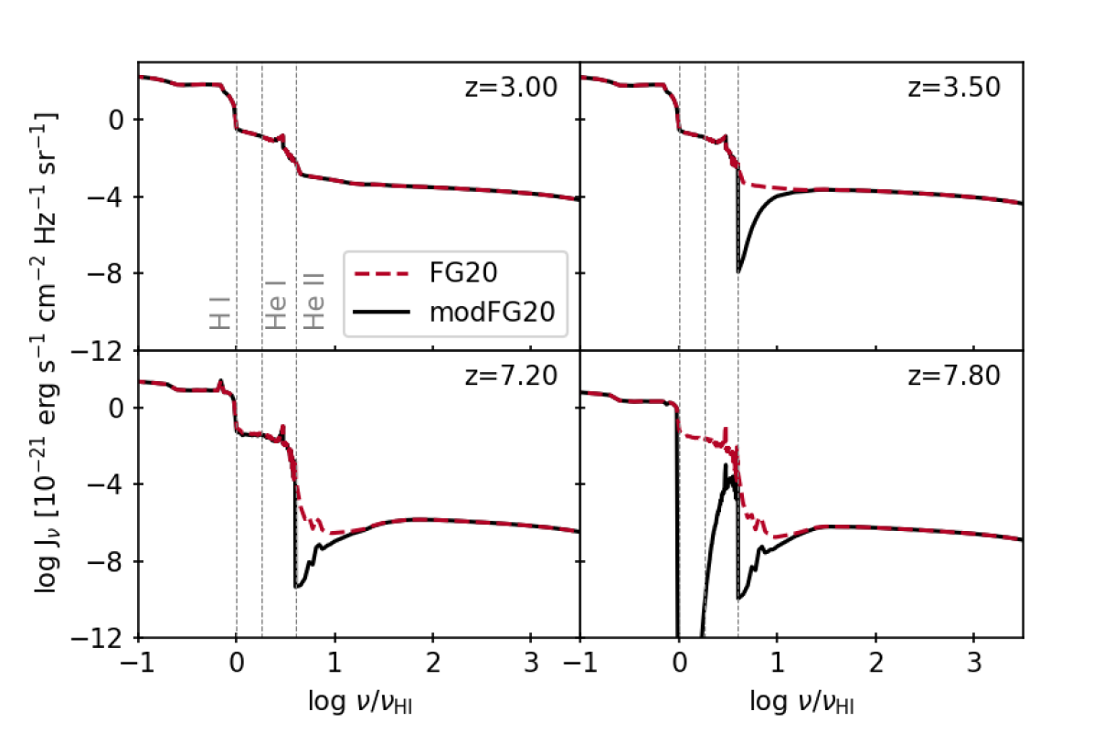
Obrázek 23: Background radiation field from FG20 (“FG20") and the modified FG20 radiation field used in this work (“modFG20") for selected redshifts after (left) and during (right) He ii (top) and H i (bottom) reionization. The vertical lines indicate the H i, He i and He ii minimum ionization energies.

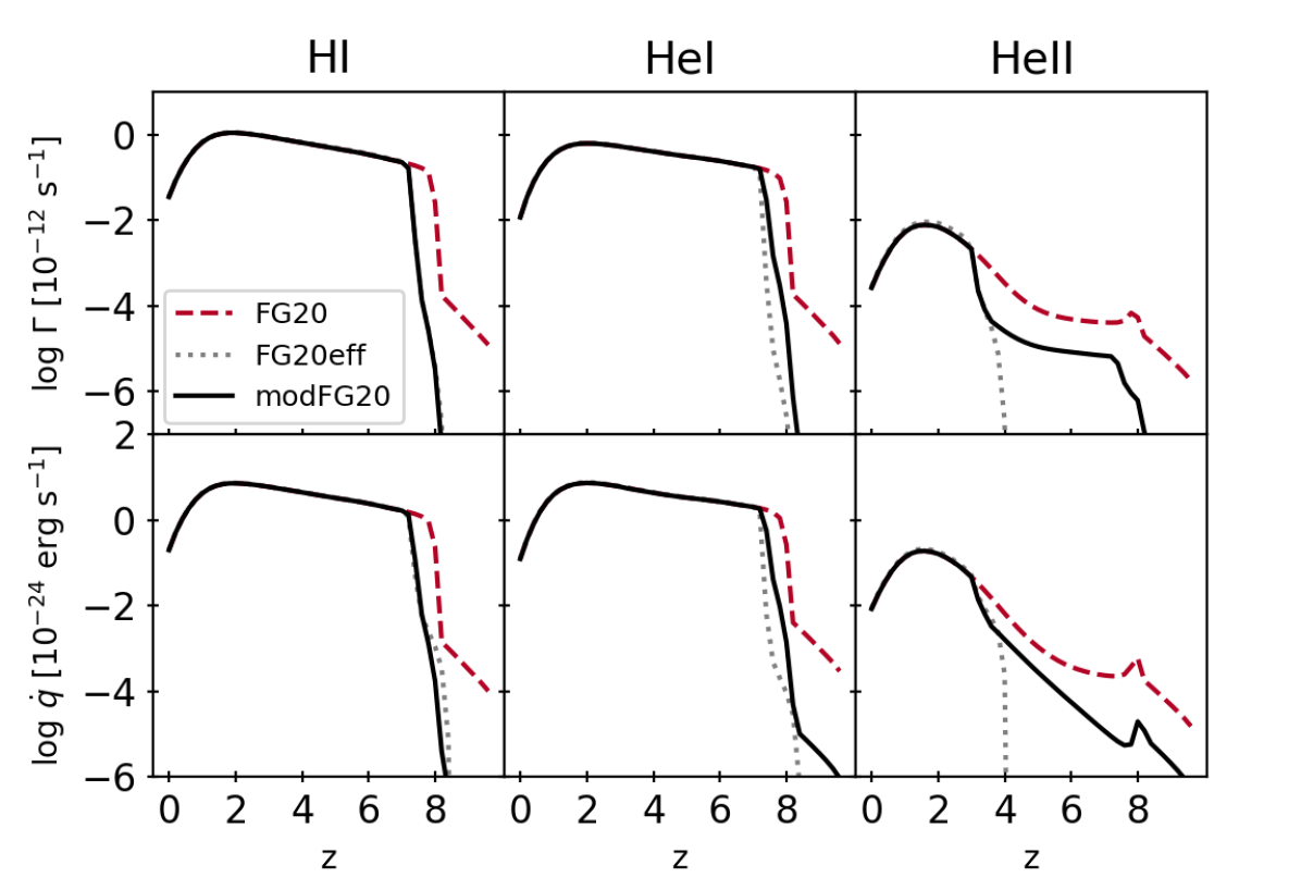
Obrázek 24: Photo-ionization (top) and photo-heating (bottom) rates for H i (left panels), He i (middle panels), and He ii (right panels) calculated from the spectrum provided from FG20 (“FG20"), the effective rates from FG20 (“FG20eff"), and calculated from the modified spectrum used in this work (“modFG20", see text for details).

Příloha C cloudy commands for reproducibility

cloudy was slightly modified to efficiently run a large grid of individual simulations with various scalings. This only involves additional command line keywords while the core calculations remain untouched. We explain in the following how standard cloudy v17.01 can be used to reproduce our results for individual grid points. Table 11 shows an example of a cloudy run with all included processes switched on (i.e. table UVB_dust1_CR1_G1_shield1). Not all command lines are present in each run (e.g. “table ISM"  is only included for tables with the ISRF).

Tabulka 11: cloudy commands for reproducing an individual grid point at redshift $z$, temperature $\log T$, metallicity $\log Z/{\mathrm{Z}}_{\odot}$ and density $\log n_{\mathrm{H}}$ from one of the tables. Column 2 lists the respective values for the arguments [value] on some command lines, e.g for the line stop column, the value from dataset ShieldingColumn for the selected grid points would be used for [value].

cloudy v17.01 command	value
constant density
constant temperature, t = [value] K log	$\log T$
hden [value]	$\log n_{\mathrm{H}}$
stop column [value] log	ShieldingColumn
abundances "solar_GASS10.abn" no grains
(or for log Z/Z⊙ = -50:
abundances "primordial.abn")
element abundance helium [value]	AbundanceHe
metals deplete
grains orion PAH [value] log no qheat	DGratio - $\log(\mathrm{D/G})_{\mathrm{0}}$
metals [value] log	$\log Z/{\mathrm{Z}}_{\odot}$
CMB redshift [value]	$z$
Table HM12 redshift [value]	$z$
table ISM [value]	RadField
cosmic rays background [value] log	CosmicRayRate - $\log\zeta_{\mathrm{0}}$
iterate to convergence
stop temperature off
Database H2

There is no direct analogue in cloudy v17.01 to scale the metal depletion, as is done in this work. But the individual depletion factors can be set manually at the bottom of file abund.cpp in the cloudy source code to $f_{\mathrm{gas,i}}=1-f_{\mathrm{dust,i}}$, with $f_{\mathrm{dust,i}}$ from the dataset Depletion.

For the UVB used here (modified FG20), replace the hm12_galaxy.ascii file in cloudy’s data folder with the provided modFG20_cloudy.ascii file, but keep the original filename (hm12_galaxy.ascii). As explained in Sec. 2.3 the dissociation rate of H₂ by CRs is re-normalized to better match the UMIST values. This has been done by changing one line in the cloudy file mole_reactions.cpp from newreact("H2,CRPHOT=>H,H","h2crphh",1.,0.,0.) to newreact("H2,CRPHOT=>H,H","h2crphh",1.746e-2,0.,0.).