Risk-Sensitive Reinforcement Learning: Near-Optimal Risk-Sample Tradeoff in Regret

Abstract

We study risk-sensitive reinforcement learning in episodic Markov decision processes with unknown transition kernels, where the goal is to optimize the total reward under the risk measure of exponential utility. We propose two provably efficient model-free algorithms, Risk-Sensitive Value Iteration (RSVI) and Risk-Sensitive Q-learning (RSQ). These algorithms implement a form of risk-sensitive optimism in the face of uncertainty, which adapts to both risk-seeking and risk-averse modes of exploration. We prove that RSVI attains an $\tilde{O}\big{(}\lambda(|\beta|H^{2})\cdot\sqrt{H^{3}S^{2}AT}\big{)}$ regret, while RSQ attains an $\tilde{O}\big{(}\lambda(|\beta|H^{2})\cdot\sqrt{H^{4}SAT}\big{)}$ regret, where $\lambda(u)=(e^{3u}-1)/u$ for $u>0$. In the above, $\beta$ is the risk parameter of the exponential utility function, $S$ the number of states, $A$ the number of actions, $T$ the total number of timesteps, and $H$ the episode length. On the flip side, we establish a regret lower bound showing that the exponential dependence on $|\beta|$ and $H$ is unavoidable for any algorithm with an $\tilde{O}(\sqrt{T})$ regret (even when the risk objective is on the same scale as the original reward), thus certifying the near-optimality of the proposed algorithms. Our results demonstrate that incorporating risk awareness into reinforcement learning necessitates an exponential cost in $|\beta|$ and $H$, which quantifies the fundamental tradeoff between risk sensitivity (related to aleatoric uncertainty) and sample efficiency (related to epistemic uncertainty). To the best of our knowledge, this is the first regret analysis of risk-sensitive reinforcement learning with the exponential utility.

1 Introduction

Risk-sensitive reinforcement learning (RL) concerns learning to act in a dynamic environment while taking into account risks that arise during the learning process. Effective management of risks in RL is critical to many real-world applications such as autonomous driving [32], real-time strategy games [56], financial investment [44], etc. In neuroscience, risk-sensitive RL has been applied to model human behaviors in decision making [46, 52].

In this paper, we consider risk-sensitive RL with the exponential utility [34] under episodic Markov decision processes (MDPs) with unknown transition kernels. Informally, the agent aims to maximize a risk-sensitive objective function of the form

$$V=\frac{1}{\beta}\log\left\{\mathbb{E}e^{\beta R}\right\},$$ (1)

where $R$ is the total reward the agent receives, and $\beta\neq 0$ is a real-valued parameter that controls risk preference of the agent; see Equation (2) for a formal definition of $V$. The objective $V$ admits the Taylor expansion $V=\mathbb{E}[R]+\frac{\beta}{2}\textup{Var}(R)+O(\beta^{2}).$ It can be seen that for $\beta>0$ the agent is risk-seeking (favoring high uncertainty in $R$), for $\beta<0$ the agent is risk-averse (favoring low uncertainty in $R$), and a larger $|\beta|$ implies higher risk-sensitivity. When $\beta\to 0$, the agent tends to be risk-neutral and the objective reduces to the expected reward objective $V=\mathbb{E}[R]$ standard in RL. Therefore, the risk-sensitive objective in (1) covers the entire spectrum of risk sensitivity by varying $\beta$. In addition, the formulation (1) is closely related to RL with constraints. For example, a negative risk parameter $\beta$ controls the tail of a risk distribution so as to mitigate the chance of receiving a total reward $R$ that is excessively low. We refer to [42, Section 2.1] for an in-depth discussion of this connection.

The challenge of risk-sensitive RL lies both in the non-linearity of the objective function and in designing a risk-aware exploration mechanism. In particular, as we elaborate in Section 2.2, the non-linear objective function (1) induces a non-linear Bellman equation. Classical RL algorithms are inappropriate in this setting, as their design crucially relies on the linearity of Bellman equations. On the other hand, effective exploration has been well known to be crucial to RL algorithm design, yet it is not clear how to design an algorithm that efficiently explores uncertain environments while at the same time adapting to the risk-sensitive objective (1) of agents with different risk parameter $\beta$.

To address these difficulties, we propose two model-free algorithms, Risk-Sensitive Value Iteration (RSVI) and Risk-Sensitive Q-learning (RSQ). Specifically, RSVI is a batch algorithm and RSQ is an online algorithm; both families of batch and online algorithms see broad applications in practice. We demonstrate in Section 3 that our proposed algorithms implement a form of risk-sensitive optimism for exploration. Importantly, the exact implementation of optimism depends on both the magnitude and the sign of the risk parameter, and therefore applies to both risk-seeking and risk-averse modes of learning. Letting $\lambda(u)=(e^{3u}-1)/u$ for $u>0$, we prove that RSVI attains an $\tilde{O}\big{(}\lambda(|\beta|H^{2})\cdot\sqrt{H^{3}S^{2}AT}\big{)}$ regret, and RSQ achieves an $\tilde{O}\big{(}\lambda(|\beta|H^{2})\cdot\sqrt{H^{4}SAT}\big{)}$ regret. Here, $S$ and $A$ are the numbers of states and actions, respectively, $T$ is the total number of timesteps, and $H$ is the length of each episode. These regret bounds interpolate across different regimes of risk sensitivity and subsume existing results under the risk-neutral setting. Compared with risk-neutral RL (corresponding to $\beta\rightarrow 0$), our general regret bounds feature an exponential dependency on $|\beta|$ and $H$, even though the risk-sensitive objective (1) is on the same scale as the total reward; see Figure 1 for a plot of the exponential factor $\lambda(|\beta|H^{2})$. Complementarily, we prove a lower bound showing that such an exponential dependency is inevitable for any algorithm and thus certifies the near-optimality of the proposed algorithms. To the best of our knowledge, our work provides the first regret analysis of risk-sensitive RL with the exponential utility.

Our upper and lower bounds demonstrate the fundamental tradeoff between risk sensitivity and sample efficiency in RL. Broadly speaking, risk sensitivity is associated with aleatoric uncertainty, which originates from the inherent randomness of state transition, actions and rewards, whereas sample efficiency is associated with epistemic uncertainty, which arises from imperfect knowledge of the environment/system and can be reduced by more exploration [24, 20]. These two notions of uncertainty are usually decoupled in the regret analysis of risk-neutral RL—in particular, using the expected reward as the objective effectively suppresses the aleatoric uncertainty. In risk-sensitive RL, we establish that there is a fundamental connection and tradeoff between these two forms of uncertainty: the risk-seeking and risk-averse regimes both incur an exponential cost in $|\beta|$ and $H$ on the regret, whereas the regret is polynomial in $H$ in the risk-neutral regime.

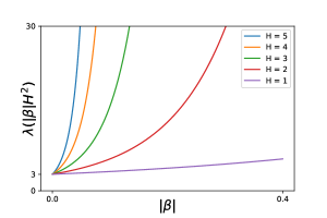
Figure 1: Scaling of $\lambda(|\beta|H^{2})$ in risk sensitivity $|\beta|$ for different values of episode length $H$.

Our contributions.

The contributions of our work can be summarized as follows:

• We consider the problem of risk-sensitive RL with the exponential utility. We propose two provably efficient model-free algorithms, namely RSVI and RSQ, that implement risk-sensitive optimism in the face of uncertainty;

• We provide regret analysis for both algorithms over the entire spectrum of risk parameter $\beta$. As $\beta\to 0$, we show that our results recover the existing regret bounds in the risk-neutral setting;

• We provide a lower bound result that certifies the near-optimality of our upper bounds and reveals a fundamental tradeoff between risk sensitivity and sample complexity.

Related work.

RL with risk-sensitive utility functions have been studied in several work. The work [45] proposes TD(0) and Q-learning-style algorithms that transform temporal differences instead of cumulative rewards, and proves their convergence. Risk-sensitive RL with a general family of utility functions is studied in [52], which also proposes a Q-learning algorithm with convergence guarantees. The work of [28] studies a risk-sensitive policy gradient algorithm, though with no theoretical guarantees. We remark that while substantial work has been devoted to designing risk-sensitive RL algorithms and proving their convergence, the issues of exploration, sample efficiency and regret bounds have rarely been studied. Our work narrows this gap in the literature by studying regret bounds of model-free algorithms for risk-sensitive RL.

The exponential utility has also been been investigated in the more classical setting of MDPs. Following the seminal work of [34], this line of work includes [7, 9, 10, 11, 14, 21, 25, 29, 30, 33, 43, 48, 51, 58]. Note that these papers impose more restrictive assumptions and study different types of results than ours. Specifically, they assume known transition kernels or access to simulators, and they do not conduct finite-time or finite-sample analysis. Another related direction to ours is RL with risk/safety constraints studied by [1, 2, 16, 19, 17, 18, 26, 27, 49, 54, 59, 61], and readers are also referred to [31] for an excellent survey on this topic. Compared to our work, that line of work focuses on constrained RL problems with different risk criteria. Other related problems include risk-sensitive games [5, 6, 8, 15, 35, 37, 40, 57], and risk-sensitive bandits [13, 23, 22, 42, 50, 53, 55, 60, 62]. Bandit problems are special cases of the RL problem that we investigate, with both the number of states and episode length being equal to one. As such, both our settings and results are more general than those obtained in bandit problems.

Notations.

For a positive integer $n$, let $[n]\coloneqq\{1,2,\ldots,n\}$. For two non-negative sequences $\{a_{i}\}$ and $\{b_{i}\}$, we write $a_{i}\lesssim b_{i}$ if there exists a universal constant $C>0$ such that $a_{i}\leq Cb_{i}$ for all $i$. We write $a_{i}\asymp b_{i}$ if $a_{i}\lesssim b_{i}$ and $b_{i}\lesssim a_{i}$. We use $\tilde{O}(\cdot)$ to denote $O(\cdot)$ while hiding logarithmic factors.

2 Problem setup

2.1 Episodic MDPs and risk-sensitive objective

We consider the setting of episodic MDPs, denoted by $\text{MDP}({\cal S},{\cal A},H,{\cal P},{\cal R})$, where ${\cal S}$ is the set of possible states, ${\cal A}$ is the set of possible actions, $H$ is the length of each episode, and ${\cal P}=\{P_{h}\}_{h\in[H]}$ and ${\cal R}=\{r_{h}\}_{h\in[H]}$ are the sets of state transition kernels and reward functions, respectively. In particular, for each $h\in[H]$, $P_{h}(\cdot\,|\,s,a)$ is the distribution of the next state if action $a$ is taken in state $s$ at step $h$. We assume that ${\cal S}$ and ${\cal A}$ are finite discrete spaces, and let $S=\left|{\cal S}\right|$ and $A=\left|{\cal A}\right|$ denote their cardinalities. We assume that the agent does not have access to $\{P_{h}\}$ and that each $r_{h}:{\cal S}\times{\cal A}\to[0,1]$ is a deterministic function.

An agent interacts with an episodic MDP as follows. At the beginning of each episode, an initial state $s_{1}$ is chosen arbitrarily by the environment. In each step $h\in[H]$, the agent observes a state $s_{h}\in{\cal S}$, chooses an action $a_{h}\in{\cal A}$, and receives a reward $r_{h}(s_{h},a_{h})$. The MDP then transitions into a new state $s_{h+1}\sim P_{h}(\cdot\,|\,s_{h},a_{h})$. We use the convention that the episode terminates when a state $s_{H+1}$ at step $H+1$ is reached, at which the agent does not take an action and receives no reward.

A policy $\pi=\{\pi_{h}\}_{h\in[H]}$ of an agent is a sequence of functions $\pi_{h}:{\cal S}\to{\cal A}$, where $\pi_{h}(s)$ is the action that the agent takes in state $s$ at step $h$ of an episode. For each $h\in[H]$, we define the value function $V_{h}^{\pi}:{\cal S}\to\mathbb{R}$ of a policy $\pi$ as the expected value of cumulative rewards the agent receives under a risk measure of exponential utility by executing policy $\pi$ starting from an arbitrary state at step $h$. Specifically, we have

$$V_{h}^{\pi}(s)\coloneqq\frac{1}{\beta}\log\left\{\mathbb{E}\left[\exp\left(\beta\sum_{h=1}^{H}r_{h}(s_{h},\pi_{h}(s_{h}))\right)\ \Bigg{|}\ s_{h}=s\right]\right\},$$ (2)

for each $(h,s)\in[H]\times{\cal S}$. Here $\beta\neq 0$ is the risk parameter of the exponential utility: $\beta>0$ corresponds to a risk-seeking value function, $\beta<0$ corresponds to a risk-averse value function, and as $\beta\to 0$ the agent tends to be risk-neutral and we recover the classical value function $V_{h}^{\pi}(s)=\mathbb{E}[\sum_{h=1}^{H}r_{h}(s_{h},\pi_{h}(s_{h}))\ |\ s_{h}=s]$ in RL. The goal of the agent is to find a policy $\pi$ such that $V_{1}^{\pi}(s)$ is maximized for all state $s\in{\cal S}$. Note the logarithm and rescaling by $1/\beta$ in the above definition, which puts the objective $V_{1}^{\pi}(s)$ on the same scale as the total reward; this scaling property is made formal in Lemma 1 below.

2.2 Bellman equations and regret

We further define the action-value function $Q_{h}^{\pi}:{\cal S}\times{\cal A}\to\mathbb{R}$, which gives the expected value of the risk measured by the exponential utility when the agent starts from an arbitrary state-action pair at step $h$ and follows policy $\pi$ afterwards; that is,

$$Q_{h}^{\pi}(s,a)\coloneqq\frac{1}{\beta}\log\left\{\exp(\beta\cdot r_{h}(s,a))\mathbb{E}\left[\exp\left(\beta\sum_{h^{\prime}=h+1}^{H}r_{h^{\prime}}(s_{h^{\prime}},a_{h^{\prime}})\right)\Bigg{|}\ s_{h}=s,a_{h}=a\right]\right\},$$

for all $(h,s,a)\in[H]\times{\cal S}\times{\cal A}$. The Bellman equation associated with policy $\pi$ is given by

$$Q_{h}^{\pi}(s,a) =r_{h}(s,a)+\frac{1}{\beta}\log\left\{\mathbb{E}_{s^{\prime}\sim P_{h}(\cdot\,|\,s,a)}\left[\exp\left(\beta\cdot V_{h+1}^{\pi}(s^{\prime})\right)\right]\right\},$$ (3)

$$V_{h}^{\pi}(s) =Q_{h}^{\pi}(s,\pi_{h}(s)),\qquad V_{H+1}^{\pi}(s)=0,$$

which holds for all $(s,a)\in{\cal S}\times{\cal A}$.

Under some mild regularity conditions, there always exists an optimal policy $\pi^{*}$ which gives the optimal value $V_{h}^{*}(s)=\sup_{\pi}V_{h}^{\pi}(s)$ for all $(h,s)\in[H]\times{\cal S}$ [7]. The Bellman optimality equation is given by

$$Q_{h}^{*}(s,a) =r_{h}(s,a)+\frac{1}{\beta}\log\left\{\mathbb{E}_{s^{\prime}\sim P_{h}(\cdot\,|\,s,a)}\left[\exp\left(\beta\cdot V_{h+1}^{*}(s^{\prime})\right)\right]\right\},$$ (4)

$$V_{h}^{*}(s) =\max_{a\in{\cal A}}Q_{h}^{*}(s,a),\qquad V_{H+1}^{*}(s)=0.$$

This equation implies that the optimal policy $\pi^{*}$ is the greedy policy with respect to the optimal action-value function $\{Q_{h}^{*}\}_{h\in[H]}$. Hence, to find the optimal policy $\pi^{*}$, it suffices to estimate the optimal action-value function. We note that both Bellman equations (3) and (4) are non-linear in the value and action-value functions due to non-linearity of the exponential utility. This is in contrast with their linear risk-neutral counterparts.

Under the episodic MDP setting, the agent aims to learn the optimal policy by interacting with the environment throughout a set of episodes. For each $k\geq 1$, let us denote by $s_{1}^{k}$ the initial state chosen by the environment and $\pi^{k}$ the policy chosen simultaneously by the agent at the beginning of episode $k$. The difference in values between $V_{1}^{\pi^{k}}(s_{1}^{k})$ and $V_{1}^{*}(s_{1}^{k})$ measures the expected regret or the sub-optimality of the agent in episode $k$. After $K$ episodes, the total regret for the agent is

$$\textup{Regret}(K) \coloneqq\sum_{k\in[K]}\left[V_{1}^{*}(s_{1}^{k})-V_{1}^{\pi^{k}}(s_{1}^{k})\right].$$ (5)

We record the following simple worst-case upper bounds on the value functions and regret.

Lemma 1.

For any $(h,s,a)\in{\cal S}\times{\cal A}\times[H]$, policy $\pi$ and risk parameter $\beta\neq 0$, we have

$$0\leq V_{h}^{\pi}(s)\leq H\quad\text{and}\quad 0\leq Q_{h}^{\pi}(s,a)\leq H.$$ (6)

Consequently, for each $K\geq 1$, all policy sequences $\pi^{1},\ldots,\pi^{K}$ and any $\beta\neq 0$, we have

$$0\leq\textup{Regret}(K)\leq KH.$$ (7)

Proof.

Recall the assumption that the reward functions $\{r_{h}\}$ are bounded in $[0,1]$. The lower bounds are immediate by definition. For the upper bound, we have $V_{h}^{\pi}(s)\leq\frac{1}{\beta}\log\left\{\mathbb{E}\left[\exp\left(\beta H\right)\right]\right\}=H.$ Upper bounds for $Q_{h}^{\pi}$ and the regret follow similarly. ∎

While straightforward, the above lemma highlights an important point: the risk and regret are on the same scale as the reward. In particular, the upper bounds above are independent of $\beta$ and linear in the horizon length $H$—the same as in the standard MDP setting—because the $\log$ and $\exp$ functions in the definition of the objective function (2) cancel with each other in the worst case. Therefore, the exponential dependence of the regret on $|\beta|$ and $H$, which we establish below in Section 4, is not merely a consequence of scaling but rather is inherent in the risk-sensitive setting.

3 Algorithms

The non-linearity of the Bellman equations, discussed in Section 2.2, creates challenges in algorithmic design. In particular, standard model-free algorithms such as least-squares value iteration (LSVI) and Q-learning are no longer appropriate since they specialize to the risk-neutral setting with linear Bellman equations. In this section, we present risk-sensitive LSVI and Q-learning algorithms that adapt to both the non-linear Bellman equations and any valid risk parameter $\beta$.

3.1 Risk-Sensitive Value Iteration

We first present Risk-Sensitive Value Iteration (RSVI) in Algorithm 1. Algorithm 1 is inspired by LSVI-UCB of [39], which is in turn motivated by the idea of LSVI [12, 47] and the classical value-iteration algorithm. Like LSVI-UCB, Algorithm 1 applies the Upper Confidence Bound (UCB) by incorporating a bonus term to value estimates of state-action pairs, which therefore implements the principle of Optimism in the Face of Uncertainty (OFU) [36].

Mechanism of Algorithm 1.

The algorithm mainly consists of the value estimation step (Line 7–14) and the policy execution step (Line 15–19). In Line 8, the algorithm computes the intermediate value $w_{h}$ by a least-squares update

$$w_{h}\leftarrow\mathop{\text{argmin}}_{w\in\mathbb{R}^{SA}}\sum_{\tau\in[k-1]}\left[e^{\beta[r_{h}(s_{h}^{\tau},a_{h}^{\tau})+V_{h+1}(s_{h+1}^{\tau})]}-w^{\top}\phi(s_{h}^{\tau},a_{h}^{\tau})\right]^{2}.$$ (8)

Here, $\{(s_{h}^{\tau},a_{h}^{\tau},s_{h+1}^{\tau})\}_{\tau\in[k-1]}$ are accessed from the dataset ${\cal D}_{h}$ for each $h\in[H]$, and $\phi(\cdot,\cdot)$ denotes the canonical basis in $\mathbb{R}^{SA}$. Line 8 can be efficiently implemented by computing sample means of $e^{\beta[r_{h}(s,a)+V_{h+1}(s^{\prime})]}$ over those state-action pairs that the algorithm has visited. Therefore, it can also be interpreted as estimating the sample means of exponentiated $Q$-values under visitation measures induced by the transition kernels $\{P_{h}\}$. This is a typical feature of the family of batch algorithms, to which Algorithm 1 belongs. Then, in Line 11, the algorithm uses the intermediate value $w_{h}$ to compute the estimate $Q_{h}$, by adding/subtracting bonus $b_{h}$ and thresholding the sum/difference at $e^{\beta(H-h+1)}$, depending on the sign of $\beta$. It is not hard to see that the logarithmic-exponential transformation in Line 11 conforms and adapts to the non-linearity in Bellman equations (3) and (4). In addition, the thresholding operator ensures that the estimated action-value function $Q_{h}$ of step $h$ stays in the range $[0,H-h+1]$ and so does the estimated value function $V_{h}$ in Line 12. This is to enforce the estimates $Q_{h}$ and $V_{h}$ to be on the same scale as the optimal $Q_{h}^{*}$ and $V_{h}^{*}$.

Besides the logarithmic-exponential transformation, another distinctive feature of Algorithm 1 is the way the bonus term $b_{h}>0$ is incorporated in Line 11. At first sight, it might appear counter-intuitive to subtract $b_{h}$ from $w_{h}$ when $\beta<0$. We demonstrate next that subtracting bonus when $\beta<0$ in fact implements the idea of OFU in a risk-sensitive fashion.

1:number of episodes $K\in\mathbb{Z}_{>0}$, confidence level $\delta\in(0,1]$, and risk parameter $\beta\neq 0$

2:$Q_{h}(s,a)\leftarrow H-h+1$ and $N_{h}(s,a)\leftarrow 0$ for all $(h,s,a)\in[H]\times{\cal S}\times{\cal A}$

3:$Q_{H+1}(s,a)\leftarrow 0$ for all $(s,a)\in{\cal S}\times{\cal A}$

4:Initialize datasets $\{{\cal D}_{h}\}$ as empty

5:for episode $k=1,\ldots,K$ do

6:     $V_{H+1}(s)\leftarrow 0$ for each $s\in{\cal S}$

7:     for step $h=H,\ldots,1$ do$\triangleright$ value estimation

8:         Update $w_{h}$ via Equation (8)

9:         for  $(s,a)\in{\cal S}\times{\cal A}$ such that $N_{h}(s,a)\geq 1$ do

10:              $b_{h}(s,a)\leftarrow c_{\gamma}\left|e^{\beta H}-1\right|\sqrt{\frac{S\log(2SAT/\delta)}{N_{h}(s,a)}}$ for some universal constant $c_{\gamma}>0$

11:              $Q_{h}(s,a)\leftarrow\begin{cases}\frac{1}{\beta}\log\left[\min\{e^{\beta(H-h+1)},w_{h}(s,a)+b_{h}(s,a)\}\right],&\text{if }\beta>0;\\ \frac{1}{\beta}\log\left[\max\{e^{\beta(H-h+1)},w_{h}(s,a)-b_{h}(s,a)\}\right],&\text{if }\beta<0\end{cases}$

12:              $V_{h}(s)\leftarrow\max_{a^{\prime}\in{\cal A}}Q_{h}(s,a^{\prime})$

13:         end for

14:     end for

15:     for  step $h=1,\ldots,H$ do$\triangleright$ policy execution

16:         Take action $a_{h}\leftarrow\mathop{\text{argmax}}_{a\in{\cal A}}Q_{h}(s_{h},a)$ and observe $r_{h}(s_{h},a_{h})$ and $s_{h+1}$

17:         $N_{h}(s_{h},a_{h})\leftarrow N_{h}(s_{h},a_{h})+1$

18:         Insert $(s_{h},a_{h},s_{h+1})$ into ${\cal D}_{h}$

19:     end for

20:end for

Algorithm 1 RSVI

Risk-Sensitive Upper Confidence Bound.

For the purpose of illustration, let us consider a “promising” state $s^{+}\in{\cal S}$ at step $h$ that allows us to transition to states {$s^{\prime}\}$ in the next step with high values $\{V_{h+1}(s^{\prime})\}$ regardless of actions taken. This means that the intermediate value $w_{h}(s^{+},\cdot)\propto\sum_{s^{\prime}}e^{\beta\cdot V_{h+1}(s^{\prime})}$ tends to be small, given that $\beta<0$ and $\{V_{h+1}(s^{\prime})\}$ are large. By subtracting a positive $b_{h}$ from $w_{h}$, we obtain an even smaller quantity $w_{h}(s^{+},\cdot)-b_{h}(s^{+},\cdot)$. We can then deduce that $Q_{h}(s^{+},\cdot)\approx\frac{1}{\beta}\log[w_{h}(s^{+},\cdot)-b_{h}(s^{+},\cdot)]$ is larger compared to $\frac{1}{\beta}\log[w_{h}(s^{+},\cdot)]$ which does not incorporate bonus, since the logarithmic function is monotonic and again $\beta<0$ (we ignore thresholding for the moment). Therefore, subtracting bonus serves as a UCB for $\beta<0$ . Since the exact form of the UCB depends on both the magnitude and sign of $\beta$ (as shown in Lines 10 and 11), we name it Risk-Sensitive Upper Confidence Bound (RS-UCB) and this results in what we call Risk-Sensitive Optimism in the Face of Uncertainty (RS-OFU).

3.2 Risk-Sensitive Q-learning

Although Algorithm 1 is model-free, it requires storage of historical data $\{{\cal D}_{h}\}$ and computation over them (Line 8). A more efficient class of algorithms is Q-learning algorithms, which update Q values in an online fashion as each state-action pair is encountered. We therefore propose Risk-Sensitive Q-learning (RSQ) and formally describe it in Algorithm 2.

1:number of episodes $K\in\mathbb{Z}_{>0}$, confidence level $\delta\in(0,1]$, learning rates $\{\alpha_{t}$} and risk parameter $\beta\neq 0$

2:$Q_{h}(s,a),V_{h}(s,a)\leftarrow H-h+1$ and $N_{h}(s,a)\leftarrow 0$ for all $(h,s,a)\in[H]\times{\cal S}\times{\cal A}$

3:$Q_{H+1}(s,a),V_{H+1}(s,a)\leftarrow 0$ for all $(s,a)\in{\cal S}\times{\cal A}$

4:for episode $k=1,\ldots,K$ do

5:     Receive the initial state $s_{1}$

6:     for step $h=1,\ldots,H$ do

7:         Take action $a_{h}\leftarrow\mathop{\text{argmax}}_{a^{\prime}\in{\cal A}}Q_{h}(s_{h},a^{\prime})$, and observe $r_{h}(s_{h},a_{h})$ and $s_{h+1}$

8:         $t=N_{h}(s_{h},a_{h})\leftarrow N_{h}(s_{h},a_{h})+1$

9:         $b_{t}\leftarrow c\left|e^{\beta H}-1\right|\sqrt{\frac{H\log(SAT/\delta)}{t}}$ for some sufficiently large universal constant $c>0$

10:         $w_{h}(s_{h},a_{h})\leftarrow(1-\alpha_{t})e^{\beta\cdot Q_{h}(s_{h},a_{h})}+\alpha_{t}e^{\beta[r_{h}(s_{h},a_{h})+V_{h+1}(s_{h+1})]}$

11:         $Q_{h}(s_{h},a_{h})\leftarrow\begin{cases}\frac{1}{\beta}\log\left[\min\{e^{\beta(H-h+1)},w_{h}(s_{h},a_{h})+\alpha_{t}b_{t}\}\right],&\text{if }\beta>0;\\ \frac{1}{\beta}\log\left[\max\{e^{\beta(H-h+1)},w_{h}(s_{h},a_{h})-\alpha_{t}b_{t}\}\right],&\text{if }\beta<0\end{cases}$

12:         $V_{h}(s_{h})\leftarrow\max_{a^{\prime}\in{\cal A}}Q_{h}(s_{h},a^{\prime})$

13:     end for

14:end for

Algorithm 2 RSQ

Mechanism of Algorithm 2.

Algorithm 2 is based on Q-learning with UCB studied in the work of [38] and we use the same learning rates therein

$$\alpha_{t}\coloneqq\frac{H+1}{H+t}$$ (9)

for every integer $t\geq 1$. Similar to Algorithm 1, Algorithm 2 consists of the policy execution step (Line 7) and value estimation step (Lines 10–12). Line 10 updates the intermediate value $w_{h}$ in an online fashion, in constrast with the batch update in Line 8 of Algorithm 1, and Algorithm 2 can thus be seen as an online algorithm. Line 11 then applies the same logarithmic-exponential transform to the intermediate value and bonu as in Algorithm 1. Note the similar way we use the bonus term $b_{t}$ in estimating $Q$-values in Line 11 of Algorithm 2 as in Line 11 of Algorithm 1. Algorithm 2 therefore also implements RS-UCB and follows the principle of RS-OFU.

Comparisons of Algorithms 1 and 2.

It is interesting to compare the bonuses used in Algorithms 1 and 2. The bonuses in both algorithms depend on the risk parameter $\beta$ through a common factor $\left|e^{\beta H}-1\right|$. A careful analysis (see our proofs in appendices) on the bonuses and the value estimation steps reveals that the effective bonuses added to the estimated value function is proportional to $\frac{e^{\left|\beta\right|H}-1}{\left|\beta\right|}$. This means that the more risk-seeking/averse an agent is (or the larger $\left|\beta\right|$ is), the larger bonus it needs to compensate for its uncertainty over the environment. Such risk sensitivity of the bonus is also reflected in the regret bounds; see Theorems 1 and 2 below. Also, it is not hard to see that both algorithms have polynomial time and space complexities in $S$, $A$, $K$ and $H$. Moreover, thanks to its online update procedure, Algorithm 2 is more efficient than Algorithms 1 in both time and space complexities, since it does not require storing historical data (in particular, $\{{\cal D}_{h}\}$ of Algorithm 1) nor computing statistics based on them for value estimation.

4 Main results

In this section, we first present regret bounds for Algorithms 1 and 2, and then we complement the results with a lower bound on regret that any algorithm has to incur.

4.1 Regret upper bounds

The following theorem gives an upper bound for regret incurred by Algorithm 1. Let $T\coloneqq KH$ be the total number of timesteps for which an algorithm is run, and recall the function $\lambda(u)\coloneqq(e^{3u}-1)/u$.

Theorem 1.

For any $\delta\in(0,1]$, with probability at least $1-\delta$, the regret of Algorithm 1 is bounded by

$$\textup{Regret}(K)\lesssim\lambda(|\beta|H^{2})\cdot\sqrt{H^{3}S^{2}AT\log^{2}(2SAT/\delta)}.$$

The proof is given in Appendix C. We see that the result of Theorem 1 adapts to both risk-seeking ($\beta>0$) and risk-averse ($\beta<0$) settings through a common factor of $\lambda(|\beta|H^{2})$.

As $\beta\to 0$, the setting of risk-sensitive RL tends to that of standard and risk-neutral RL, and we have an immediate corollary to Theorem 1 as a precise characterization.

Corollary 1.

Under the setting of Theorem 1 and when $\beta\to 0$, with probability at least $1-\delta$, the regret of Algorithm 1 is bounded by

$$\textup{Regret}(K) \lesssim\sqrt{H^{3}S^{2}AT\log^{2}(2SAT/\delta)}.$$

Proof.

The result follows from Theorem 1 and the fact that $\lim_{\beta\to 0}\lambda(|\beta|H^{2})=3$. ∎

The result in Corollary 1 recovers the regret bound of [4, Theorem 2] under the standard RL setting and is nearly optimal compared to the minimax rates presented in [3, Theorems 1 and 2]. Corollary 1 also reveals that Theorem 1 interpolates between the risk-sensitive and risk-neutral settings.

Next, we give a regret upper bound for Algorithm 2 in the following theorem.

Theorem 2.

For any $\delta\in(0,1]$, with probability at least $1-\delta$ and when $T$ is sufficiently large, the regret of Algorithm 2 is bounded by

$$\textup{Regret}(K) \lesssim\ \lambda(|\beta|H^{2})\cdot\sqrt{H^{4}SAT\log(SAT/\delta)}.$$

The proof is given in Appendix E. Similarly to Theorem 1, Theorem 2 also covers both risk-seeking and risk-averse settings via the same factor $\lambda(|\beta|H^{2})$, which gives the risk-neutral bound when $\beta\to 0$ as shown in the following.

Corollary 2.

Under the setting of Theorem 2 and when $\beta\to 0$, with probability at least $1-\delta$, the regret of Algorithm 2 is bounded by

$$\textup{Regret}(K) \lesssim\sqrt{H^{4}SAT\log(SAT/\delta)}.$$

The proof follows the same reasoning as in that of Corollary 1. According to Corollary 2, the regret upper bound for Algorithm 2 matches the nearly optimal result in [38, Theorem 2] under the risk-neutral setting. As such, Theorems 1 and 2 strictly generalizes the existing nearly optimal regret bounds (up to polynomial factors).

The crux of the proofs of both Theorems 1 and 2 lies in a local linearization argument for the non-linear Bellman equations and non-linear updates of the algorithms, in which action-value and value functions are related by a logarithmic-exponential transformation. Although logarithmic and exponential functions are not Lipschitz globally, we show that they are locally Lipschitz in the domain of our interest, and their combined local Lipschitz factors turn out to be the exponential factors in the theorems. Once the Bellman equations and algorithm estimates are linearized, we can apply standard techniques in RL to obtain the final regret. It is noteworthy that, as suggested by [38], the regret bounds in Theorems 1 and 2 can automatically be translated into sample complexity bounds in the probably approximately correct (PAC) setting, which did not previously exist even given access to a simulator.

In the risk-sensitive setting where $\beta$ is bounded away from $0$, our regret bounds of Theorems 1 and 2 depend exponentially in the horizon length $H$ and the risk sensitivity $|\beta|$. In what follows, we argue that such exponential dependence is unavoidable.

4.2 Regret lower bound

We now present a fundamental lower bound on the regret, which complements the upper bounds in Theorems 1 and 2.

Theorem 3.

For sufficiently large $K$ and $H$, the regret of any algorithm obeys

$$\mathbb{E}\left[\textup{Regret}(K)\right] \gtrsim\frac{e^{\left|\beta\right|H/2}-1}{\left|\beta\right|}\sqrt{T\log T}.$$

The proof is given in Appendix F. In the proof, we construct a bandit model that can be seen as a special case of our episodic fixed-horizon MDP problem, and then we show that any bandit algorithm has to incur an expected regret, in terms of the logarithmic-exponential objective, that grows as predicted in Theorem 3.

Theorem 3 shows that the exponential dependence on the $|\beta|$ and $H$ in Theorems 1 and 2 is essentially indispensable. In addition, it features a sub-linear dependence on $T$ through the $\tilde{O}(\sqrt{T})$ factor. In view of Theorem 3, therefore, both Theorems 1 and 2 are nearly optimal in their dependence on $\beta$, $H$ and $T$. One should contrast Theorem 3 with Lemma 1, which shows that the worst-case regret is linear in $H$ and $T$. Such a linear regret can be attained by any trivial algorithm that does not learn at all. In sharp contrast, in order to achieve the optimal $\sqrt{T}$ scaling (which by standard arguments implies a finite sample-complexity bound), an algorithm must incur a regret that is exponential in $H$. Therefore, our results show a (perhaps surprising) tradeoff between risk sensitivity and sample efficiency.

Appendix A Preliminaries

We set some notations and shorthands before the proofs. For both Algorithms 1 and 2, we let $s_{h}^{k}$, $a_{h}^{k}$, $w_{h}^{k}$, $Q_{h}^{k}$ and $V_{h}^{k}$ denote the values of $s_{h}$, $a_{h}$, $w_{h}$, $Q_{h}$ and $V_{h}$ in episode $k$, and we denote by $N_{h}^{k}$ the value of $N_{h}$ at the end of episode $k-1$. For Algorithm 1, we let ${\cal D}_{h}^{k}$ be the value of ${\cal D}_{h}$ at the end of episode $k-1$. Next, we introduce a simple yet powerful result.

Fact 1.

Consider $x,y,b\in\mathbb{R}$ such that $x\geq y$.

1. if $y\geq g$ for some $g>0$, then $\log(x)-\log(y)\leq\frac{1}{g}(x-y)$;

2. Assume further that $y\geq 0$. If $b\geq 0$ and $x\leq u$ for some $u>0$, then $e^{bx}-e^{by}\leq be^{bu}(x-y)$; if $b<0$, then $e^{by}-e^{bx}\leq(-b)(x-y)$.

Proof.

The results follow from Lipschitz continuity of the functions $x\mapsto\log(x)$ and $x\mapsto e^{bx}$. ∎

We record a simple fact about exponential factors.

Fact 2.

Define $\lambda_{0}\coloneqq\frac{e^{\left|\beta\right|H}-1}{\left|\beta\right|}$ and $\lambda_{2}\coloneqq e^{\left|\beta\right|(H^{2}+H)}$. Then we have $\lambda_{0}\lambda_{2}H\leq\frac{e^{3\left|\beta\right|H^{2}}-1}{\left|\beta\right|}$.

Appendix B Proof warmup for Theorem 1

First, we set some notations and definitions. Define $d\coloneqq SA$, $\iota\coloneqq\log(2dT/\delta)$ for a given $\delta\in(0,1]$, and $I$ to be the $d\times d$ identity matrix. To streamline some parts of the proof, we define $\phi(s,a)$ to be a vector in $\mathbb{R}^{d}$ whose $(s,a)$-th entry is equal to one and other entries equal to zero (so $\phi(s,a)$ is a canonical basis of $\mathbb{R}^{SA}$). Also let $\Lambda_{h}^{k}$ be a diagonal matrix in $\mathbb{R}^{d\times d}$ with each $(s,a)$-th diagonal entry equal to $\max\{N_{h}^{k-1}(s,a),1\}$. It can be seen that $\Lambda_{h}^{k}$ is positive definite. We adopt the shorthands $\phi_{h}^{\tau}\coloneqq\phi(s_{h}^{\tau},a_{h}^{\tau})$ and $r_{h}^{\tau}\coloneqq r_{h}(s_{h}^{\tau},a_{h}^{\tau})$ for $(\tau,h)\in[K]\times[H]$.

From now on, we fix a tuple $(k,h)\in[K]\times[H]$ and then fix $(s,a)\in{\cal S}\times{\cal A}$ such that $N_{h}^{k-1}(s,a)\geq 1$. We also fix a policy $\pi$. We set

$$w_{h}^{\pi}=e^{\beta\cdot Q_{h}^{\pi}(\cdot,\cdot)}.$$ (10)

It can be verified that by the definition of $\phi(s,a)$, we have

$$Q_{h}^{\pi}(s,a) =\frac{1}{\beta}\log\left(e^{\beta\cdot Q_{h}^{\pi}(s,a)}\right)$$

$$=\frac{1}{\beta}\log\left(\left\langle\phi(s,a),e^{\beta\cdot Q_{h}^{\pi}(\cdot,\cdot)}\right\rangle\right)$$

$$=\frac{1}{\beta}\log\left(\left\langle\phi(s,a),w_{h}^{\pi}\right\rangle\right),$$ (11)

as well as

$$w_{h}^{\pi}(s,a) =e^{\beta\cdot Q_{h}^{\pi}(s,a)}=\left\langle\phi(s,a),(\Lambda_{h}^{k})^{-1}\sum_{\tau\in[k-1]}\phi_{h}^{\tau}\left[e^{\beta\cdot Q_{h}^{\pi}(s_{h}^{\tau},a_{h}^{\tau})}\right]\right\rangle,$$ (12)

where the last step follows from the definition of $\Lambda_{h}^{k}$.

Let us define

$$q_{1}^{+} \coloneqq\begin{cases}\left\langle\phi(s,a),w_{h}^{k}\right\rangle+b_{h}^{k}(s,a),&\text{if }\beta>0,\\ \left\langle\phi(s,a),w_{h}^{k}\right\rangle-b_{h}^{k}(s,a),&\text{if }\beta<0,\end{cases}$$

$$q_{1} \coloneqq\begin{cases}\min\{e^{\beta(H-h+1)},q_{1}^{+}\},&\text{if }\beta>0,\\ \max\{e^{\beta(H-h+1)},q_{1}^{+}\},&\text{if }\beta<0.\end{cases}$$

By the definition of $\Lambda_{h}^{k}$ and $\phi_{h}^{k}$, observe that

$$w_{h}^{k}(s,a)=\left\langle\phi(s,a),w_{h}^{k}\right\rangle=\left\langle\phi(s,a),(\Lambda_{h}^{k})^{-1}\sum_{\tau\in[k-1]}\phi_{h}^{\tau}\left[e^{\beta[r_{h}^{\tau}+V_{h+1}^{k}(s_{h+1}^{\tau})]}\right]\right\rangle.$$ (13)

Define

$$G_{0}\coloneqq(Q_{h}^{k}-Q_{h}^{\pi})(s,a)=\frac{1}{\beta}\log\left\{q_{1}\right\}-\frac{1}{\beta}\log\left\{\left\langle\phi(s,a),w_{h}^{\pi}\right\rangle\right\},$$ (14)

and our goal is to derive lower and upper bounds for $G_{0}$. From Equation (14), we have

$$G_{0} =\frac{1}{\beta}\log\left\{q_{1}\right\}-\frac{1}{\beta}\log\left\{\left\langle\phi(s,a),(\Lambda_{h}^{k})^{-1}\sum_{\tau\in[k-1]}\phi_{h}^{\tau}\left[e^{\beta\cdot Q_{h}^{\pi}(s_{h}^{\tau},a_{h}^{\tau})}\right]\right\rangle\right\}$$

$$=\frac{1}{\beta}\log\left\{q_{1}\right\}-\frac{1}{\beta}\log\left\{\left\langle\phi(s,a),(\Lambda_{h}^{k})^{-1}\sum_{\tau\in[k-1]}\phi_{h}^{\tau}\left[\mathbb{E}_{s^{\prime}\sim P_{h}(\cdot\,|\,s_{h}^{\tau},a_{h}^{\tau})}e^{\beta[r_{h}^{\tau}+V_{h+1}^{\pi}(s^{\prime})]}\right]\right\rangle\right\}$$

$$\eqqcolon\frac{1}{\beta}\log\{q_{1}\}-\frac{1}{\beta}\log\{q_{3}\}.$$

The first step above holds by Equation (12), and the second step follows from Equation (3). In order to control $G_{0}$, we define an intermediate quantity

$$q_{2}\coloneqq\left\langle\phi(s,a),(\Lambda_{h}^{k})^{-1}\sum_{\tau\in[k-1]}\phi_{h}^{\tau}\left[\mathbb{E}_{s^{\prime}\sim P_{h}(\cdot\,|\,s_{h}^{\tau},a_{h}^{\tau})}e^{\beta[r_{h}^{\tau}+V_{h+1}^{k}(s^{\prime})]}\right]\right\rangle;$$

in words, $q_{2}$ replaces the quantity $V_{h+1}^{\pi}$ in $q_{3}$ by $V_{h+1}^{k}$. It can be seen that

$$G_{0}=G_{1}+G_{2},$$ (15)

where

$$G_{1} \coloneqq\frac{1}{\beta}\log\{q_{1}\}-\frac{1}{\beta}\log\{q_{2}\},$$ (16)

$$G_{2} \coloneqq\frac{1}{\beta}\log\{q_{2}\}-\frac{1}{\beta}\log\{q_{3}\}.$$

Note that $G_{0}$, $G_{1}$ and $G_{2}$ are all well-defined, according to the following result.

Lemma 2.

We have $q_{i}\in[\min\{1,e^{\beta(H-h+1)}\},\max\{1,e^{\beta(H-h+1)}\}]$ for $i\in[3]$.

Proof.

We prove the result by focusing on $q_{1}$. By the definitions of $\Lambda_{h}^{k}$ and $\phi$, the $(s,a)$-th entry of the vector $(\Lambda_{h}^{k})^{-1}\sum_{\tau\in[k-1]}\phi_{h}^{\tau}\cdot u_{h}^{\tau}$ equals $\frac{1}{N_{h}^{k-1}(s,a)}\sum_{\tau\in[k-1]}u_{h}^{\tau}\cdot\mathbb{I}\{(s_{h}^{\tau},a_{h}^{\tau})=(s,a)\}$ for any sequence $\{u_{h}^{\tau}\}_{\tau\in[k-1]}$. Then, the result follows from the fact that $e^{\beta[r_{h}^{\tau}+V_{h+1}^{k}(s^{\prime})]}\in[\min\{1,e^{\beta(H-h)}\},\max\{1,e^{\beta(H-h)}\}]$ for $(\tau,s^{\prime})\in[K]\times{\cal S}$ and the definition of $q_{1}$. ∎

Therefore, we have the following equivalent form of Equation (14):

$$(Q_{h}^{k}-Q_{h}^{\pi})(s,a)=G_{1}+G_{2}.$$ (17)

Thanks to the identity (17), our goal is now to control $G_{1}$ and $G_{2}$, which is done in the following lemma.

Lemma 3.

For all $(k,h,s,a)\in[K]\times[H]\times{\cal S}\times{\cal A}$ that satisifies $N_{h}^{k-1}(s,a)\geq 1$, there exist universal constants $c_{1},c_{\gamma}>0$ (where $c_{\gamma}$ is used in Line 10 of Algorithm 1) such that

$$0\leq G_{1}\leq c_{1}\cdot\frac{e^{\left|\beta\right|H}-1}{\left|\beta\right|}\cdot d\sqrt{\iota}\sqrt{\phi(s,a)^{\top}(\Lambda_{h}^{k})^{-1}\phi(s,a)}$$

with probability at least $1-\delta/2$. Furthermore, if $V_{h+1}^{k}(s^{\prime})\geq V_{h+1}^{\pi}(s^{\prime})$ for all $s^{\prime}\in{\cal S}$, then we have

$$0\leq G_{2}\leq e^{\left|\beta\right|H}\cdot\mathbb{E}_{s^{\prime}\sim P_{h}(\cdot\,|\,s,a)}[V_{h+1}^{k}(s^{\prime})-V_{h+1}^{\pi}(s^{\prime})].$$

Proof.

Case $\beta>0$. To control $G_{1}$, we note that $N_{h}^{k-1}(s,a)=\phi(s,a)^{\top}(\Lambda_{h}^{k})^{-1}\phi(s,a)$ and by Equation (13) we can compute

$$\quad\left|q_{1}^{+}-q_{2}-b_{h}^{k}(s,a)\right|$$

$$=\left|\left\langle\phi(s,a),(\Lambda_{h}^{k})^{-1}\sum_{\tau\in[k-1]}\phi_{h}^{\tau}\left[e^{\beta[r_{h}^{\tau}+V_{h+1}^{k}(s_{h+1}^{\tau})]}-\mathbb{E}_{s^{\prime}\sim P_{h}(\cdot\,|\,s_{h}^{\tau},a_{h}^{\tau})}e^{\beta[r_{h}^{\tau}+V_{h+1}^{k}(s^{\prime})]}\right]\right\rangle\right|$$

$$=\left|\frac{1}{N_{h}^{k-1}(s,a)}\sum_{(s,a,s^{+})\in{\cal D}_{h}^{k-1}}e^{\beta[r_{h}(s,a)+V_{h+1}^{k}(s^{+})]}-\mathbb{E}_{s^{\prime}\sim P_{h}(\cdot\,|\,s,a)}e^{\beta[r_{h}(s,a)+V_{h+1}^{k}(s^{\prime})]}\right|$$

$$\leq\frac{1}{N_{h}^{k-1}(s,a)}\sum_{(s,a,s^{+})\in{\cal D}_{h}^{k-1}}\left|e^{\beta[r_{h}(s,a)+V_{h+1}^{k}(s^{+})]}-\mathbb{E}_{s^{\prime}\sim P_{h}(\cdot\,|\,s,a)}e^{\beta[r_{h}(s,a)+V_{h+1}^{k}(s^{\prime})]}\right|$$

$$\leq\frac{1}{N_{h}^{k-1}(s,a)}\sum_{t\in\left[N_{h}^{k-1}(s,a)\right]}c^{\prime}\left|e^{\beta H}-1\right|\sqrt{\frac{S\iota}{t}}$$

$$\leq\frac{1}{N_{h}^{k-1}(s,a)}\int_{t\in\left[0,N_{h}^{k-1}(s,a)\right]}c^{\prime}\left|e^{\beta H}-1\right|\sqrt{\frac{S\iota}{t}}\mathrm{d}t$$

$$=\frac{1}{N_{h}^{k-1}(s,a)}\cdot c\left|e^{\beta H}-1\right|\sqrt{S\iota\cdot N_{h}^{k-1}(s,a)}$$

$$=c\left|e^{\beta H}-1\right|\sqrt{S\iota}\cdot\sqrt{\phi(s,a)^{\top}(\Lambda_{h}^{k})^{-1}\phi(s,a)},$$

where the fourth step holds by Lemma 6, and the last step holds by the definition of $\Lambda_{h}^{k}$; in the above, $c^{\prime}>0$ is a universal constant and $c=2c^{\prime}$. If we choose $c_{\gamma}=c$ in the definition of $b_{h}^{k}(s,a)$ in Line 10 of Algorithm 1, we have

$$0\leq q_{1}^{+}-q_{2}\leq 2c\cdot\left|e^{\beta H}-1\right|\sqrt{S\iota}\cdot\sqrt{\phi(s,a)^{\top}(\Lambda_{h}^{k})^{-1}\phi(s,a)}.$$

Therefore, we have $q_{1}\geq q_{2}$, and thus $G_{1}\geq 0$, by the first inequality above, the definition of $q_{1}$ and Lemma 2 (in particular, $q_{2}\leq e^{\beta(H-h+1)}$). By Lemma 2 and Fact 1(a) (with $g=1$, $x=q_{1}$ and $y=q_{2}$), we have

$$G_{1}\leq\frac{1}{\beta}(q_{1}-q_{2})\leq\frac{1}{\beta}(q_{1}^{+}-q_{2}),$$

which together with the second inequality displayed above implies the desired upper bound on $G_{1}$.

Now we control the term $G_{2}$. For $\beta>0$, it is not hard to see that the assumption $V_{h+1}^{k}(s^{\prime})\geq V_{h+1}^{\pi}(s^{\prime})$ for all $s^{\prime}\in{\cal S}$ implies that $q_{2}\geq q_{3}$ and therefore $G_{2}\geq 0$. We also have

$$G_{2} \leq\frac{1}{\beta}(q_{2}-q_{3})$$

$$\leq e^{\beta H}\left\langle\phi(s,a),(\Lambda_{h}^{k})^{-1}\sum_{\tau\in[k-1]}\phi_{h}^{\tau}\left[\mathbb{E}_{s^{\prime}\sim P_{h}(\cdot\,|\,s_{h}^{\tau},a_{h}^{\tau})}[V_{h+1}^{k}(s^{\prime})-V_{h+1}^{\pi}(s^{\prime})]\right]\right\rangle$$

$$=e^{\left|\beta\right|H}\mathbb{E}_{s^{\prime}\sim P_{h}(\cdot\,|\,s,a)}[V_{h+1}^{k}(s^{\prime})-V_{h+1}^{\pi}(s^{\prime})],$$

where the first step holds by Fact 1(a) (with $g=1$, $x=q_{2}$, and $y=q_{3}$) and the fact that $q_{2}\geq q_{3}\geq 1$ (with the last inequality suggested by Lemma 2), and the second step holds by Fact 1(b) (with $b=\beta$, $x=r_{h}^{\tau}+V_{h+1}^{k}(s)$, and $y=r_{h}^{\tau}+V_{h+1}^{\pi}(s)$) and $H\geq r_{h}^{\tau}+V_{h+1}^{k}(s)\geq r_{h}^{\tau}+V_{h+1}^{\pi}(s)\geq 0$.

Case $\beta<0$. Similar to the case of $\beta>0$, we have

$$\quad\left|q_{1}^{+}-q_{2}+b_{h}^{k}(s,a)\right|$$

$$\leq c\cdot\left|e^{\beta H}-1\right|\sqrt{S\iota}\cdot\sqrt{\phi(s,a)^{\top}(\Lambda_{h}^{k})^{-1}\phi(s,a)}.$$

If we choose $c_{\gamma}=c$ in the definition of $b_{h}^{k}(s,a)$ in Line 10 of Algorithm 1, the above equation implies

$$0\leq q_{2}-q_{1}^{+}\leq 2c\cdot\left|e^{\beta H}-1\right|\sqrt{S\iota}\cdot\sqrt{\phi(s,a)^{\top}(\Lambda_{h}^{k})^{-1}\phi(s,a)}.$$

Therefore, we have $q_{1}\leq q_{2}$, and thus $G_{1}\geq 0$, by the first inequality displayed above, the definition of $q_{1}$ and Lemma 2 (in particular, $q_{2}\geq e^{\beta(H-h+1)}$). By Lemma 2 and Fact 1(a) (with $g=e^{\beta H}$, $x=q_{2}$ and $y=q_{1})$, we further have

$$G_{1} =\frac{1}{(-\beta)}\left(\log\{q_{2}\}-\log\{q_{1}\}\right)$$

$$\leq\frac{e^{-\beta H}}{\left|\beta\right|}(q_{2}-q_{1})$$

$$\leq\frac{e^{-\beta H}}{\left|\beta\right|}(q_{2}-q_{1}^{+}),$$

which together with the second inequality displayed above and the fact that $\left|e^{\beta H}-1\right|=1-e^{\beta H}$ implies the desired upper bound on $G_{1}$.

Next we control $G_{2}$. The assumption $V_{h+1}^{k}(s^{\prime})\geq V_{h+1}^{\pi}(s^{\prime})$ for all $s^{\prime}\in{\cal S}$ implies that $q_{2}\leq q_{3}$ and therefore $G_{2}\geq 0$. We also have

$$G_{2} =\frac{1}{(-\beta)}\left(\log\{q_{3}\}-\log\{q_{2}\}\right)$$

$$\leq\frac{e^{-\beta H}}{(-\beta)}(q_{3}-q_{2})$$

$$\leq e^{\left|\beta\right|H}\left\langle\phi(s,a),(\Lambda_{h}^{k})^{-1}\sum_{\tau\in[k-1]}\phi_{h}^{\tau}\left[\mathbb{E}_{s^{\prime}\sim P_{h}(\cdot\,|\,s_{h}^{\tau},a_{h}^{\tau})}[V_{h+1}^{k}(s^{\prime})-V_{h+1}^{\pi}(s^{\prime})]\right]\right\rangle$$

$$=e^{\left|\beta\right|H}\mathbb{E}_{s^{\prime}\sim P_{h}(\cdot\,|\,s,a)}[V_{h+1}^{k}(s^{\prime})-V_{h+1}^{\pi}(s^{\prime})],$$

where the second step holds by Fact 1(a) (with $g=e^{\beta H}$, $x=q_{3}$, and $y=q_{2}$) and the fact that $q_{3}\geq q_{2}\geq e^{\beta H}$ (with the last inequality suggested by Lemma 2), and the third step holds by Fact 1(b) (with $b=\beta$, $x=r_{h}^{\tau}+V_{h+1}^{k}(s)$, and $y=r_{h}^{\tau}+V_{h+1}^{\pi}(s)$) and $r_{h}^{\tau}+V_{h+1}^{k}(s)\geq r_{h}^{\tau}+V_{h+1}^{\pi}(s)\geq 0$.

The proof is hence completed. ∎

The next lemma establishes the dominance of $Q^{k}_{h}$ over $Q^{*}_{h}$.

Lemma 4.

On the event of Lemma 3, we have $Q_{h}^{k}(s,a)\geq Q_{h}^{\pi}(s,a)$ for all $(k,h,s,a)\in[K]\times[H]\times{\cal S}\times{\cal A}$.

Proof.

For the purpose of the proof, we set $Q_{H+1}^{\pi}(s,a)=Q_{H+1}^{*}(s,a)=0$ for all $(s,a)\in{\cal S}\times{\cal A}$. We fix a tuple $(k,s,a)\in[K]\times{\cal S}\times{\cal A}$ and use strong induction on $h$. The base case for $h=H+1$ is satisfied since $(Q_{H+1}^{k}-Q_{H+1}^{\pi})(s,a)=0$ for $k\in[K]$ by definition. Now we fix an $h\in[H]$ and assume that $0\leq(Q_{h+1}^{k}-Q_{h+1}^{*})(s,a)$. Moreover, by the induction assumption we have

$$V_{h+1}^{k}(s)=\max_{a^{\prime}\in{\cal A}}Q_{h+1}^{k}(s,a^{\prime})\geq\max_{a^{\prime}\in{\cal A}}Q_{h+1}^{\pi}(s,a^{\prime})\geq V_{h+1}^{\pi}(s).$$ (18)

We also assume that $(s,a)$ satisfies $N_{h}^{k-1}(s,a)\geq 1$, since otherwise $Q_{h}^{k}(s,a)=H-h+1\geq Q_{h}^{\pi}(s,a)$ and we are done. This assumption and Equation (18) together imply $G_{2}\geq 0$ by Lemma 3. We also have $G_{1}\geq 0$ on the event of Lemma 3. Therefore, it follows that $(Q_{h}^{k}-Q_{h}^{\pi})(s,a)\geq 0$ by Equation (17). The induction is completed and so is the proof. ∎

Lemma 4 leads to an immediate and important corollary.

Lemma 5.

For any $\delta\in(0,1]$, with probability at least $1-\delta/2$, we have $V_{h}^{k}(s)\geq V_{h}^{\pi}(s)$ for all $(k,h,s)\in[K]\times[H]\times{\cal S}$.

Proof.

The result follows from Lemma 4 and Equation (18). ∎

B.1 Supporting lemmas

We first present a concentration result.

Lemma 6.

Define

$$\bar{{\cal V}}_{h+1}\coloneqq\left\{\bar{V}_{h+1}:{\cal S}\to\mathbb{R}\mid\forall s\in{\cal S},\ \bar{V}_{h+1}(s)\in[\min\{e^{\beta(H-h)},1\},\max\{e^{\beta(H-h)},1\}]\right\}.$$

There exists a universal constant $c>0$ such that with probability $1-\delta$, we have

$$\left|e^{\beta[r_{h}(s_{h}^{k},a_{h}^{k})+\bar{V}(s_{h+1}^{k})]}-\mathbb{E}_{s^{\prime}\sim P_{h}(\cdot\mid s_{h}^{k},a_{h}^{k})}e^{\beta[r_{h}(s_{h}^{k},a_{h}^{k})+\bar{V}(s^{\prime})]}\right|\leq c\left|e^{\beta H}-1\right|\sqrt{\frac{S\iota}{N_{h}^{k}(s,a)}}$$

for all $(k,h,s,a)\in[K]\times[H]\times{\cal S}\times{\cal A}$ and all $\bar{V}\in\bar{{\cal V}}_{h+1}$.

Proof.

The proof follows the same reasoning as [4, Lemma 12]. ∎

The next few lemmas help control $\sum_{k\in[K]}(\phi_{h}^{k})^{\top}(\Lambda_{h}^{k})^{-1}\phi_{h}^{k}$.

Lemma 7 ([39, Lemma D.2]).

Let $\{\phi_{t}\}_{t\geq 0}$ be a bounded sequence in $\mathbb{R}^{d}$ satisfying $\sup_{t\geq 0}\|\phi_{t}\|\leq 1$. Let $\Lambda_{0}\in\mathbb{R}^{d\times d}$ be a positive definite matrix with $\lambda_{\min}(\Lambda_{0})\geq 1$. For any $t\geq 0$, we define $\Lambda_{t}\coloneqq\Lambda_{0}+\sum_{i\in[t]}\phi_{i}\phi_{i}^{\top}$. Then, we have

$$\log\left[\frac{\det(\Lambda_{t})}{\det(\Lambda_{0})}\right]\leq\sum_{i\in[t]}\phi_{i}^{\top}\Lambda_{i-1}^{-1}\phi_{i}\leq 2\log\left[\frac{\det(\Lambda_{t})}{\det(\Lambda_{0})}\right].$$

Lemma 8.

Recall the definitions of $\phi_{h}^{k}$ and $\Lambda_{h}^{k}$. For any $h\in[H]$, we have

$$\sum_{k\in[K]}(\phi_{h}^{k})^{\top}(\Lambda_{h}^{k})^{-1}\phi_{h}^{k}\leq 2d\iota,$$

where $\iota=\log(2dT/\delta)$

Proof.

Define $\Gamma_{h}^{k}\coloneqq\lambda I+\sum_{\tau\in[k-1]}\phi_{h}^{\tau}(\phi_{h}^{\tau})^{\top}$ with $\lambda=1$. It is not hard to see that by the definition of $\Lambda_{h}^{k}$ we have $\Lambda_{h}^{k}\preceq\Gamma_{h}^{k}$ for $h\in[H]$. Since $\lambda_{\min}(\Gamma_{h}^{k})\geq 1$ and $\|\phi_{h}^{k}\|\leq 1$ for all $(k,h)\in[K]\times[H]$, by Lemma 7 we have for any $h\in[H]$ that

$$\sum_{k\in[K]}(\phi_{h}^{k})^{\top}(\Lambda_{h}^{k})^{-1}\phi_{h}^{k}\leq\sum_{k\in[K]}(\phi_{h}^{k})^{\top}(\Gamma_{h}^{k})^{-1}\phi_{h}^{k}\leq 2\log\left[\frac{\det(\Gamma_{h}^{k+1})}{\det(\Gamma_{h}^{1})}\right].$$

Furthermore, note that $\|\Gamma_{h}^{k+1}\|=\|\lambda I+\sum_{\tau\in[k]}\phi_{h}^{k}(\phi_{h}^{k})^{\top}\|\leq\lambda+k$. This implies

$$\sum_{k\in[K]}(\phi_{h}^{k})^{\top}(\Lambda_{h}^{k})^{-1}\phi_{h}^{k}\leq 2d\log\left[\frac{\lambda+k}{\lambda}\right]\leq 2d\iota,$$

as desired. ∎

Appendix C Proof of Theorem 1

Define $\delta_{h}^{k}\coloneqq V_{h}^{k}(s_{h}^{k})-V_{h}^{\pi_{k}}(s_{h}^{k})$, and $\zeta_{h+1}^{k}\coloneqq\mathbb{E}_{s^{\prime}\sim P_{h}(\cdot\,|\,s_{h}^{k},a_{h}^{k})}[V_{h+1}^{k}(s^{\prime})-V_{h+1}^{\pi_{k}}(s^{\prime})]-\delta_{h+1}^{k}$. For any $(k,h)\in[K]\times[H]$, we have

$$\delta_{h}^{k} =(Q_{h}^{k}-Q_{h}^{\pi_{k}})(s_{h}^{k},a_{h}^{k})$$

$$\leq c_{1}\cdot\frac{e^{\left|\beta\right|H}-1}{\left|\beta\right|}\cdot\sqrt{S\iota}\sqrt{\phi(s_{h}^{k},a_{h}^{k})^{\top}(\Lambda_{h}^{k})^{-1}\phi(s_{h}^{k},a_{h}^{k})}$$

$$\quad+e^{\left|\beta\right|H}\cdot\mathbb{E}_{s^{\prime}\sim P_{h}(\cdot\,|\,s_{h}^{k},a_{h}^{k})}[V_{h+1}^{k}(s^{\prime})-V_{h+1}^{\pi_{k}}(s^{\prime})]$$

$$=c_{1}\cdot\frac{e^{\left|\beta\right|H}-1}{\left|\beta\right|}\cdot\sqrt{S\iota}\sqrt{\phi(s_{h}^{k},a_{h}^{k})^{\top}(\Lambda_{h}^{k})^{-1}\phi(s_{h}^{k},a_{h}^{k})}$$

$$\quad+e^{\left|\beta\right|H}(\delta_{h+1}^{k}+\zeta_{h+1}^{k}).$$ (19)

In the above equation, the first step holds by the construction of Algorithm 1 and the definition of $V_{h}^{\pi_{k}}$ in Equation (3); the second step is a consequence of combining Equation (17) as well as Lemmas 3 and 5; the last step follows from the definitions of $\delta_{h}^{k}$ and $\zeta_{h+1}^{k}$.

Noting that $V_{H+1}^{k}(s)=V_{H+1}^{\pi_{k}}(s)=0$ and the fact that $\delta_{h+1}^{k}+\zeta_{h+1}^{k}\geq 0$ implied by Lemma 5, we can continue by expanding the recursion in Equation (19) and get

$$\delta_{1}^{k} \leq\sum_{h\in[H]}e^{(\left|\beta\right|H)h}\zeta_{h+1}^{k}$$

$$\quad+c_{1}\cdot\frac{e^{\left|\beta\right|H}-1}{\left|\beta\right|}\cdot\sum_{h\in[H]}e^{(\left|\beta\right|H)(h-1)}\sqrt{S\iota}\sqrt{\phi(s_{h}^{k},a_{h}^{k})^{\top}(\Lambda_{h}^{k})^{-1}\phi(s_{h}^{k},a_{h}^{k})}.$$ (20)

Therefore, we have

$$\textup{Regret}(K) =\sum_{k\in[K]}\left[(V_{1}^{*}-V_{1}^{\pi_{k}})(s_{1}^{k})\right]$$

$$\leq\sum_{k\in[K]}\delta_{1}^{k}$$

$$\leq e^{\left|\beta\right|H^{2}}\sum_{k\in[K]}\sum_{h\in[H]}\zeta_{h+1}^{k}$$

$$\quad+c_{1}\cdot\frac{e^{\left|\beta\right|H}-1}{\left|\beta\right|}\cdot e^{\left|\beta\right|H^{2}}\cdot\sqrt{S\iota}\sum_{k\in[K]}\sum_{h\in[H]}\sqrt{\phi(s_{h}^{k},a_{h}^{k})^{\top}(\Lambda_{h}^{k})^{-1}\phi(s_{h}^{k},a_{h}^{k})},$$ (21)

where the second step holds by Lemma 5 with $\pi$ therein set to the optimal policy, and in the last step we applied Equation (20) along with the Cauchy-Schwarz inequality.

We proceed to control the two terms in Equation (21). Since the construction of $V_{h}^{k}$ is independent of the new observation $s_{h}^{k}$ in episode $k$, we have that $\{\zeta_{h+1}^{k}\}$ is a martingale difference sequence satisfying $\left|\zeta_{h}^{k}\right|\leq 2H$ for all $(k,h)\in[K]\times[H]$. By the Azuma-Hoeffding inequality, we have for any $t>0$,

$$\mathbb{P}\left(\sum_{k\in[K]}\sum_{h\in[H]}\zeta_{h+1}^{k}\geq t\right)\leq\exp\left(-\frac{t^{2}}{2T\cdot H^{2}}\right).$$

Hence, with probability $1-\delta/2$, there holds

$$\sum_{k\in[K]}\sum_{h\in[H]}\zeta_{h+1}^{k}\leq\sqrt{2TH^{2}\cdot\log(2/\delta)}\leq 2H\sqrt{T\iota},$$ (22)

where $\iota=\log(2dT/\delta)$. For the second term in Equation (21), we apply Lemma 8 and the Cauchy-Schwarz inequality to obtain

$$\quad\sum_{k\in[K]}\sum_{h\in[H]}\sqrt{\phi(s_{h}^{k},a_{h}^{k})^{\top}(\Lambda_{h}^{k})^{-1}\phi(s_{h}^{k},a_{h}^{k})}$$

$$\leq\sum_{h\in[H]}\sqrt{K}\sqrt{\sum_{k\in[H]}\phi(s_{h}^{k},a_{h}^{k})^{\top}(\Lambda_{h}^{k})^{-1}\phi(s_{h}^{k},a_{h}^{k})}$$

$$\leq H\sqrt{2dK\iota}.$$ (23)

Plugging Equations (22) and (23) back to Equation (21) yields

$$\textup{Regret}(K) \leq e^{\left|\beta\right|H^{2}}\cdot 2H\sqrt{T\iota}+c_{1}\cdot\frac{e^{\left|\beta\right|H}-1}{\left|\beta\right|}\cdot e^{\left|\beta\right|H^{2}}\cdot H\sqrt{2dSK\iota^{2}}$$

$$\leq(c_{1}+2)\cdot\frac{e^{\left|\beta\right|H}-1}{\left|\beta\right|}\cdot e^{\left|\beta\right|H^{2}}\cdot\sqrt{2dHST\iota^{2}},$$

where the last step holds since $\frac{e^{\left|\beta\right|H}-1}{\left|\beta\right|}\geq H$. The proof is completed in view of Fact 2 and the identity $d=SA$.

Appendix D Proof warmup for Theorem 2

Recall the learning rates $\{\alpha_{t}\}$ defined in Equation (9). Define the quantities

$$\alpha_{t}^{0}\coloneqq\prod_{j=1}^{t}(1-\alpha_{j}),\qquad\alpha_{t}^{i}\coloneqq\alpha_{i}\prod_{j=i+1}^{t}(1-\alpha_{j})$$ (24)

for integers $i,t\geq 1$. By convention, we set $\alpha_{t}^{0}=1$ and $\sum_{i\in[t]}\alpha_{t}^{i}=0$ if $t=0$, and $\alpha_{t}^{i}=\alpha_{i}$ if $t<i+1$. Define the shorthand $\iota\coloneqq\log(SAT/\delta)$ for $\delta\in(0,1]$.

The following fact describes some key properties of the learning rates $\{\alpha_{t}\}$.

Fact 3.

The following properties hold for $\alpha_{t}^{i}$.

1. $\frac{1}{\sqrt{t}}\leq\sum_{i\in[t]}\frac{\alpha_{t}^{i}}{\sqrt{i}}\leq\frac{2}{\sqrt{t}}$ for every integer $t\geq 1$.

2. $\max_{i\in[t]}\alpha_{t}^{i}\leq\frac{2H}{t}$ and $\sum_{i\in[t]}(\alpha_{t}^{i})^{2}\leq\frac{2H}{t}$ for every integer $t\geq 1$.

3. $\sum_{t=i}^{\infty}\alpha_{t}^{i}=1+\frac{1}{H}$ for every integer $i\geq 1$.

4. $\sum_{i\in[t]}\alpha_{t}^{i}=1$ and $\alpha_{t}^{0}=0$ for every integer $t\geq 1$, and $\sum_{i\in[t]}\alpha_{t}^{i}=0$ and $\alpha_{t}^{0}=1$ for $t=0$.

Proof.

The first three facts can be found in [38, Lemma 4.1], and the last one follows from direct calculation in view of Equation (24). ∎

We also present a lemma that controls the deviation of the exponentiated value function from its expectation.

Lemma 9.

There exists a universal constant $c>0$ such that for any $(k,h,s,a)\in[K]\times[H]\times{\cal S}\times{\cal A}$ and $k_{1},\ldots,k_{t}<k$ with $t=N_{h}^{k}(s,a)$, we have

$$\quad\left|\frac{1}{\beta}\sum_{i\in[t]}\alpha_{t}^{i}\left[e^{\beta[r_{h}(s,a)+V_{h+1}^{*}(s_{h+1}^{k_{i}})]}-\mathbb{E}_{s^{\prime}\sim P_{h}(\cdot\,|\,s,a)}e^{\beta[r_{h}(s,a)+V_{h+1}^{*}(s^{\prime})]}\right]\right|$$

$$\leq\frac{c\left|e^{\beta H}-1\right|}{\left|\beta\right|}\sqrt{\frac{H\iota}{t}}.$$

with probability at least $1-\delta$, and

$$\frac{1}{\left|\beta\right|}\sum_{i\in[t]}\alpha_{t}^{i}b_{i}\in\left[\frac{c\left|e^{\beta H}-1\right|}{\left|\beta\right|}\sqrt{\frac{H\iota}{t}},\frac{2c\left|e^{\beta H}-1\right|}{\left|\beta\right|}\sqrt{\frac{H\iota}{t}}\right].$$

Proof.

For any $(k,h,s,a)\in[K]\times[H]\times{\cal S}\times{\cal A}$, define

$$\psi(i,k,h,s,a)\coloneqq e^{\beta[r_{h}(s,a)+V_{h+1}^{*}(s_{h+1}^{k_{i}})]}-\mathbb{E}_{s^{\prime}\sim P_{h}(\cdot\,|\,s,a)}e^{\beta[r_{h}(s,a)+V_{h+1}^{*}(s^{\prime})]}$$

Let us fix a tuple $(k,h,s,a)\in[K]\times[H]\times{\cal S}\times{\cal A}$. It can be seen that $\{\mathbb{I}(k_{i}\leq K)\cdot\psi(i,k,h,s,a)\}_{i\in[\tau]}$ for $\tau\in[K]$ is a martingale difference sequence. By the Azuma-Hoeffding inequality and a union bound over $\tau\in[K]$, we have with probability at least $1-\delta/(HSA)$, for all $\tau\in[K]$,

$$\left|\sum_{i\in[\tau]}\alpha_{\tau}^{i}\cdot\mathbb{I}(k_{i}\leq K)\cdot\psi(i,k,h,s,a)\right|$$

$$\leq\frac{c\left|e^{\beta H}-1\right|}{2}\sqrt{\iota\sum_{i\in[\tau]}(\alpha_{\tau}^{i})^{2}}\leq c\left|e^{\beta H}-1\right|\sqrt{\frac{H\iota}{\tau}}$$

where $c>0$ is some universal constant, the first step holds since $r_{h}(s,a)+V_{h+1}^{*}(s^{\prime})\in[0,H]$ for $s^{\prime}\in{\cal S}$, and the last step follows from Fact 3(b). Since the above equation holds for all $\tau\in[K]$, it also holds for $\tau=t=N_{h}^{k}(s,a)\leq K$. Note that $\mathbb{I}(k_{i}\leq K)=1$ for all $i\in[N_{h}^{k}(s,a)]$. Therefore, applying another union bound over $(h,s,a)\in[H]\times{\cal S}\times{\cal A}$, we have that the following holds for all $(k,h,s,a)\in[K]\times[H]\times{\cal S}\times{\cal A}$ and with probability at least $1-\delta$:

$$\left|\sum_{i\in[t]}\alpha_{\tau}^{i}\cdot\psi(i,k,h,s,a)\right| \leq c\left|e^{\beta H}-1\right|\sqrt{\frac{H\iota}{t}},$$ (25)

where $t=N_{h}^{k}(s,a)$. Using the fact that $r_{h}+V_{h+1}^{*}\in[0,H]$, we have

$$\quad\left|\frac{1}{\beta}\sum_{i\in[t]}\alpha_{t}^{i}\left[\mathbb{E}_{s^{\prime}\sim\hat{P}_{h}^{k_{i}}(\cdot\,|\,s,a)}e^{\beta[r_{h}(s,a)+V_{h+1}^{*}(s^{\prime})]}-\mathbb{E}_{s^{\prime}\sim P_{h}(\cdot\,|\,s,a)}e^{\beta[r_{h}(s,a)+V_{h+1}^{*}(s^{\prime})]}\right]\right|$$

$$=\left|\frac{1}{\beta}\sum_{i\in[t]}\alpha_{t}^{i}\cdot\psi(i,k,h,s,a)\right|\leq\frac{c\left|e^{\beta H}-1\right|}{\left|\beta\right|}\sqrt{\frac{H\iota}{t}}.$$

To prove the result for $\frac{1}{\left|\beta\right|}\sum_{i\in[t]}\alpha_{t}^{i}b_{i}$, we recall the definition of $\{b_{t}\}$ in Line 9 of Algorithm 2 and compute

$$\frac{1}{\left|\beta\right|}\sum_{i\in[t]}\alpha_{t}^{i}b_{i} =\frac{c\left|e^{\beta H}-1\right|}{\left|\beta\right|}\sum_{i\in[t]}\alpha_{t}^{i}\sqrt{\frac{H\iota}{i}}$$

$$\in\left[\frac{c\left|e^{\beta H}-1\right|}{\left|\beta\right|}\sqrt{\frac{H\iota}{t}},\frac{2c\left|e^{\beta H}-1\right|}{\left|\beta\right|}\sqrt{\frac{H\iota}{t}}\right]$$

where the last step holds by Fact 3(a). ∎

We fix a tuple $(k,h,s,a)\in[K]\times[H]\times{\cal S}\times{\cal A}$ with $k_{i}\leq k$ being the episode in which $(s,a)$ is taken the $i$-th time at step $h$. Let us define

$$q_{1}^{+} \coloneqq\begin{cases}\alpha_{t}^{0}e^{\beta(H-h+1)}+\sum_{i\in[t]}\alpha_{t}^{i}\left[e^{\beta[r_{h}(s,a)+V_{h+1}^{k_{i}}(s_{h+1}^{k_{i}})]}+b_{i}\right],&\text{if }\beta>0,\\ \alpha_{t}^{0}e^{\beta(H-h+1)}+\sum_{i\in[t]}\alpha_{t}^{i}\left[e^{\beta[r_{h}(s,a)+V_{h+1}^{k_{i}}(s_{h+1}^{k_{i}})]}-b_{i}\right],&\text{if }\beta<0,\end{cases}$$

$$q_{1} \coloneqq\begin{cases}\min\{e^{\beta(H-h+1)},q_{1}^{+}\},&\text{if }\beta>0,\\ \max\{e^{\beta(H-h+1)},q_{1}^{+}\},&\text{if }\beta<0,\end{cases}$$

and

$$q_{2}^{+} \coloneqq\begin{cases}\alpha_{t}^{0}e^{\beta(H-h+1)}+\sum_{i\in[t]}\alpha_{t}^{i}\left[e^{\beta[r_{h}(s,a)+V_{h+1}^{*}(s_{h+1}^{k_{i}})]}+b_{i}\right],&\text{if }\beta>0,\\ \alpha_{t}^{0}e^{\beta(H-h+1)}+\sum_{i\in[t]}\alpha_{t}^{i}\left[e^{\beta[r_{h}(s,a)+V_{h+1}^{*}(s_{h+1}^{k_{i}})]}-b_{i}\right],&\text{if }\beta<0,\end{cases}$$

$$q_{2} \coloneqq\begin{cases}\min\{e^{\beta(H-h+1)},q_{2}^{+}\},&\text{if }\beta>0,\\ \max\{e^{\beta(H-h+1)},q_{2}^{+}\},&\text{if }\beta<0,\end{cases}$$

$$q_{2}^{\prime} \coloneqq\alpha_{t}^{0}e^{\beta(H-h+1)}+\sum_{i\in[t]}\alpha_{t}^{i}\left[e^{\beta[r_{h}(s,a)+V_{h+1}^{*}(s_{h+1}^{k_{i}})]}\right],$$

and

$$q_{3}\coloneqq\alpha_{t}^{0}e^{\beta\cdot Q_{h}^{*}(s,a)}+\sum_{i\in[t]}\alpha_{t}^{i}\left[\mathbb{E}_{s^{\prime}\sim P_{h}(\cdot\,|\,s,a)}e^{\beta[r_{h}(s,a)+V_{h+1}^{*}(s^{\prime})]}\right].$$

We have a simple fact on $q_{2}$ and $q_{2}^{\prime}$.

Fact 4.

If $\beta>0$, we have $q_{2}^{\prime}\leq q_{2}$; if $\beta<0$, we have $q_{2}^{\prime}\geq q_{2}$.

Proof.

We focus on the case of $\beta>0$. Note that $r_{h}(s,a)+V_{h+1}^{*}(s_{h+1}^{k_{i}})\in[0,H-h+1]$, which implies $e^{\beta[r_{h}(s,a)+V_{h+1}^{*}(s_{h+1}^{k_{i}})]}\leq e^{\beta(H-h+1)}$. We also have $\alpha_{t}^{0},\sum_{i\in[t]}\alpha_{t}^{i}\in\{0,1\}$ with $\alpha_{t}^{0}+\sum_{i\in[t]}\alpha_{t}^{i}=1$ by Fact 3(d). These together imply that $q_{2}^{\prime}\leq e^{\beta H}$ and $q_{2}^{\prime}-q_{2}^{+}=-\sum_{i\in[t]}\alpha_{t}^{i}b_{i}\leq 0$ by definition of $b_{i}$ in Line 9 of Algorithm 2. Therefore, $q_{2}^{\prime}\leq\min\{e^{\beta(H-h+1)},q_{2}^{+}\}=q_{2}$. The case of $\beta<0$ can be proved in a similar way and thus omitted. ∎

Next, we establish a representation of the performance difference $(Q_{h}^{k}-Q_{h}^{*})(s,a)$ using the quantities $q_{1}$ and $q_{3}$.

Lemma 10.

For any $(k,h,s,a)\in[K]\times[H]\times{\cal S}\times{\cal A}$, let $t=N_{h}^{k}(s,a)$ and suppose $(s,a)$ was previously taken at step $h$ of episodes $k_{1},\ldots,k_{t}<k$. We have

$$(Q_{h}^{k}-Q_{h}^{*})(s,a)=\frac{1}{\beta}\log\{q_{1}\}-\frac{1}{\beta}\log\{q_{3}\}.$$

Proof.

The Bellman optimality equation (4) implies

$$e^{\beta\cdot Q_{h}^{*}(s,a)}=e^{\beta\cdot r_{h}(s,a)}\left[\mathbb{E}_{s^{\prime}\sim P_{h}(\cdot\,|\,s,a)}e^{\beta\cdot V_{h+1}^{*}(s^{\prime})}\right].$$

By Fact 3(d), we have

$$e^{\beta\cdot Q_{h}^{*}(s,a)} =\alpha_{t}^{0}e^{\beta\cdot Q_{h}^{*}(s,a)}+\sum_{i\in[t]}\alpha_{t}^{i}e^{\beta\cdot r_{h}(s,a)}\left[\mathbb{E}_{s^{\prime}\sim P_{h}(\cdot\,|\,s,a)}e^{\beta\cdot V_{h+1}^{*}(s^{\prime})}\right]=q_{3}$$

for each integer $t\geq 0$, and therefore

$$Q_{h}^{*}(s,a) =\frac{1}{\beta}\log\left\{q_{3}\right\}.$$ (26)

We finish the proof by combining Equation (26) and the fact that $Q_{h}^{k}(s,a)=\frac{1}{\beta}\log\{q_{1}\}$, which follows from Line 11 of Algorithm 2. ∎

We define the quantities

$$G_{1} \coloneqq\frac{1}{\beta}\log\{q_{1}\}-\frac{1}{\beta}\log\{q_{2}\},$$ (27)

$$G_{2} \coloneqq\frac{1}{\beta}\log\{q_{2}\}-\frac{1}{\beta}\log\{q_{3}\},$$

It is not hard to see that $(Q_{h}^{k}-Q_{h}^{*})(s,a)=G_{1}+G_{2}$ by Lemma 10. The next lemma establishes upper and lower bounds for $(Q_{h}^{k}-Q_{h}^{*})(s,a)$.

Lemma 11.

For all $(k,h,s,a)\in[K]\times[H]\times{\cal S}\times{\cal A}$ such that $t=N_{h}^{k}(s,a)\geq 1$, let

$$\gamma_{t}\coloneqq 2\sum_{i\in[t]}\alpha_{t}^{i}b_{i}\cdot\begin{cases}\frac{1}{\left|\beta\right|},&\text{if }\beta>0,\\ \frac{e^{-\beta H}}{\left|\beta\right|},&\text{if }\beta<0,\end{cases}$$

and with probability at least $1-\delta$ we have

$$0\leq(Q_{h}^{k}-Q_{h}^{*})(s,a) \leq\alpha_{t}^{0}He^{\left|\beta\right|H}+\sum_{i\in[t]}\alpha_{t}^{i}e^{\left|\beta\right|H}\left[V_{h+1}^{k_{i}}(s_{h+1}^{k_{i}})-V_{h+1}^{*}(s_{h+1}^{k_{i}})\right]+2\gamma_{t},$$

where $k_{1},\ldots,k_{t}<k$ are the episodes in which $(s,a)$ was taken at step $h$, and $\gamma_{t}\leq\frac{4c(e^{\left|\beta\right|H}-1)}{\left|\beta\right|}\sqrt{\frac{H\iota}{t}}$.

Proof.

We prove the lower bound for $(Q_{h}^{k}-Q_{h}^{*})(s,a)$ and then use it to prove the upper bound.

Lower bound for $Q^{k}-Q^{*}$.

For the purpose of the proof, we set $Q_{H+1}^{k}(s,a)=Q_{H+1}^{*}(s,a)=0$ for all $(k,s,a)\in[K]\times{\cal S}\times{\cal A}$. We fix a $(s,a)\in{\cal S}\times{\cal A}$ and use strong induction on $k$ and $h$. Without loss of generality, we assume that there exists a $(k,h)$ such that $(s,a)=(s_{h}^{k},a_{h}^{k})$ (that is, $(s,a)$ has been taken at some point in Algorithm 2), since otherwise $Q_{h}^{k}(s,a)=H-h+1\geq Q_{h}^{*}(s,a)$ for all $(k,h)\in[K]\times[H]$ and we are done. The base case for $k=1$ and $h=H+1$ is satisfied since $(Q_{H+1}^{k^{\prime}}-Q_{H+1}^{*})(s,a)=0$ for $k^{\prime}\in[K]$ by definition. We fix a $(k,h)\in[K]\times[H]$ and assume that $0\leq(Q_{h+1}^{k_{i}}-Q_{h+1}^{*})(s,a)$ for each $k_{1},\ldots,k_{t}<k$ (here $t=N_{h}^{k}(s,a)$). Then we have for $i\in[t]$ that

$$V_{h+1}^{k_{i}}(s)=\max_{a^{\prime}\in{\cal A}}Q_{h+1}^{k_{i}}(s,a^{\prime})\geq\max_{a^{\prime}\in{\cal A}}Q_{h+1}^{*}(s,a^{\prime})=V_{h+1}^{*}(s).$$

Recall the quantities $G_{1}$ and $G_{2}$ defined in Equation (27). The above equation implies $G_{1}\geq 0$. We also have $G_{2}\geq 0$ by the fact $Q_{h}^{*}(s,a)\leq H$ and on the event of Lemma 9. Therefore, it follows that $(Q_{h}^{k}-Q_{h}^{*})(s,a)=G_{1}+G_{2}\geq 0$. The induction is completed and we have proved that $0\leq(Q_{h}^{k}-Q_{h}^{*})(s,a)$ for all $(k,h,s,a)\in[K]\times[H]\times{\cal S}\times{\cal A}$.

Upper bound for $Q^{k}-Q^{*}$.

Let us fix a $(k,h,s,a)\in[K]\times[H]\times{\cal S}\times{\cal A}$. Since $0\leq(Q_{h}^{k}-Q_{h}^{*})(s,a)$, we have for $i\in[t]$ that

$$V_{h+1}^{k_{i}}(s)=\max_{a^{\prime}\in{\cal A}}Q_{h+1}^{k_{i}}(s,a^{\prime})\geq\max_{a^{\prime}\in{\cal A}}Q_{h+1}^{*}(s,a^{\prime})=V_{h+1}^{*}(s).$$

Case $\beta>0$. We have

$$G_{1} =\frac{1}{\beta}\log\{q_{1}\}-\frac{1}{\beta}\log\{q_{2}\}$$

$$\leq\frac{1}{\beta}(q_{1}-q_{2})$$

$$\leq\frac{1}{\beta}(q_{1}^{+}-q_{2}^{\prime})$$

$$\leq\frac{1}{\beta}\sum_{i\in[t]}\alpha_{t}^{i}\left[e^{\beta[r_{h}(s,a)+V_{h+1}^{k_{i}}(s_{h+1}^{k_{i}})]}-e^{\beta[r_{h}(s,a)+V_{h+1}^{*}(s_{h+1}^{k_{i}})]}\right]+\frac{1}{\beta}\sum_{i\in[t]}\alpha_{t}^{i}b_{i}$$

$$\leq e^{\left|\beta\right|H}\sum_{i\in[t]}\alpha_{t}^{i}\left[(V_{h+1}^{k_{i}}-V_{h+1}^{*})(s_{h+1}^{k_{i}})\right]+\gamma_{t},$$

where the second step holds by Fact 1(a) with $g=1$ and the fact that $V_{h+1}^{k_{i}}(s)\geq V_{h+1}^{*}(s)$ and by noticing that $\alpha_{t}^{0},\sum_{i\in[t]}\alpha_{t}^{i}\in\{0,1\}$ with $\alpha_{t}^{0}+\sum_{i\in[t]}\alpha_{t}^{i}=1$ by Fact 3(d) (so that $q_{1}\geq q_{2}$), the third step holds since by definition $q_{1}^{+}\geq q_{1}$ and by Fact 4 $q_{2}^{\prime}\leq q_{2}$, and the last step holds by Fact 1(b) and the fact that $H\geq r_{h}(s,a)+V_{h+1}^{k_{i}}(s)\geq r_{h}(s,a)+V_{h+1}^{*}(s)\geq 0$. For $G_{2}$, we have

$$G_{2} =\frac{1}{\beta}\log\{q_{2}\}-\frac{1}{\beta}\log\{q_{3}\}$$

$$\leq\frac{1}{\beta}(q_{2}-q_{3})$$

$$\leq\frac{1}{\beta}(q_{2}^{+}-q_{3})$$

$$=\frac{\alpha_{t}^{0}}{\beta}\left[e^{\beta H}-e^{\beta\cdot Q_{h}^{*}(s,a)}\right]+\frac{1}{\beta}\sum_{i\in[t]}\alpha_{t}^{i}b_{i}$$

$$\quad+\frac{1}{\beta}\sum_{i\in[t]}\alpha_{t}^{i}\left[e^{\beta[r_{h}(s,a)+V_{h+1}^{*}(s_{h+1}^{k_{i}})]}-\mathbb{E}_{s^{\prime}\sim P_{h}(\cdot\,|\,s,a)}e^{\beta[r_{h}(s,a)+V_{h+1}^{*}(s^{\prime})]}\right]$$

$$\leq\alpha_{t}^{0}He^{\left|\beta\right|H}+\gamma_{t},$$

In the above, the second step holds by Fact 1(a) with $g=1$ and

$$\sum_{i\in[t]}\alpha_{t}^{i}b_{i}\geq\left|\sum_{i\in[t]}\alpha_{t}^{i}\left[e^{\beta[r_{h}(s,a)+V_{h+1}^{*}(s_{h+1}^{k_{i}})]}-\mathbb{E}_{s^{\prime}\sim P_{h}(\cdot\,|\,s,a)}e^{\beta[r_{h}(s,a)+V_{h+1}^{*}(s^{\prime})]}\right]\right|$$

on the event of Lemma 9 (so that $q_{2}\geq q_{3}$); the third step holds by Fact 4; the last step holds by Fact 1(b) and $Q_{h}^{*}(s,a)\in[0,H]$ and on the event of Lemma 9.

Case $\beta<0$. We have

$$G_{1} =\frac{1}{(-\beta)}\log\{q_{2}\}-\frac{1}{(-\beta)}\log\{q_{1}\}$$

$$\leq\frac{e^{-\beta H}}{(-\beta)}(q_{2}-q_{1})$$

$$\leq\frac{e^{-\beta H}}{(-\beta)}(q_{2}^{\prime}-q_{1}^{+})$$

$$=\frac{e^{-\beta H}}{(-\beta)}\sum_{i\in[t]}\alpha_{t}^{i}\left[e^{\beta[r_{h}(s,a)+V_{h+1}^{*}(s_{h+1}^{k_{i}})]}-e^{\beta[r_{h}(s,a)+V_{h+1}^{k_{i}}(s_{h+1}^{k_{i}})]}\right]+\frac{e^{-\beta H}}{(-\beta)}\sum_{i\in[t]}\alpha_{t}^{i}b_{i}$$

$$\leq e^{\left|\beta\right|H}\sum_{i\in[t]}\alpha_{t}^{i}\left[(V_{h+1}^{k_{i}}-V_{h+1}^{*})(s_{h+1}^{k_{i}})\right]+\gamma_{t},$$

where the second step holds by Fact 1(a) with $g=e^{\beta H}$ and the fact that $V_{h+1}^{k_{i}}(s)\geq V_{h+1}^{*}(s)$ (so that $q_{2}\geq q_{1}$), the third step holds since $q_{2}^{\prime}\geq q_{2}$ by Fact 4 and $q_{1}^{+}\leq q_{1}$ by definition, and the last step holds by Fact 1(b) and the fact that $H\geq r_{h}(s,a)+V_{h+1}^{k_{i}}(s)\geq r_{h}(s,a)+V_{h+1}^{*}(s)\geq 0$. For $G_{2}$, we have

$$G_{2} =\frac{1}{(-\beta)}\log\{q_{3}\}-\frac{1}{(-\beta)}\log\{q_{2}\}$$

$$\leq\frac{e^{-\beta H}}{(-\beta)}(q_{3}-q_{2})$$

$$\leq\frac{e^{-\beta H}}{(-\beta)}(q_{3}-q_{2}^{+})$$

$$=\frac{e^{-\beta H}}{(-\beta)}\alpha_{t}^{0}\left[e^{\beta\cdot Q_{h}^{*}(s,a)}-e^{\beta H}\right]+\frac{e^{-\beta H}}{(-\beta)}\sum_{i\in[t]}\alpha_{t}^{i}b_{i}$$

$$\quad+\frac{e^{-\beta H}}{(-\beta)}\sum_{i\in[t]}\alpha_{t}^{i}\left[\mathbb{E}_{s^{\prime}\sim P_{h}(\cdot\,|\,s,a)}e^{\beta[r_{h}(s,a)+V_{h+1}^{*}(s^{\prime})]}-e^{\beta[r_{h}(s,a)+V_{h+1}^{*}(s_{h+1}^{k_{i}})]}\right]$$

$$\leq e^{-\beta H}\alpha_{t}^{0}\left[H-Q_{h}^{*}(s,a)\right]+\frac{2e^{-\beta H}}{(-\beta)}\sum_{i\in[t]}\alpha_{t}^{i}b_{i}$$

$$\leq\alpha_{t}^{0}He^{\left|\beta\right|H}+\gamma_{t}.$$

where the second step holds by Fact 1(a) given $q_{3}\geq q_{2}$, the second to the last step holds by Fact 1(b), the fact that $Q_{h}^{*}(s,a)\leq H$ and on the event of Lemma 9, and the last step holds by the definition of $\gamma_{t}$.

Combining the bounds of $G_{1}$ and $G_{2}$ with the identity $(Q_{h}^{k}-Q_{h}^{*})(s,a)=G_{1}+G_{2}$ yields the upper bound for $(Q_{h}^{k}-Q_{h}^{*})(s,a)$. The proof is completed in view of Lemma 9 and the definition of $\gamma_{t}$ that imply

$$\gamma_{t}\leq\frac{4c(e^{\left|\beta\right|H}-1)}{\left|\beta\right|}\sqrt{\frac{H\iota}{t}}.$$

∎

Appendix E Proof of Theorem 2

We first introduce some notations. Let ${\cal G}$ be a discrete space. Define the shorthand

$$\mathsf{lse}_{\beta}(P,f)\coloneqq\frac{1}{\beta}\log\left\{\mathbb{E}_{x\sim P}\left[\exp\left(\beta\cdot f(x)\right)\right]\right\},$$ (28)

for a probability distribution $P$ supported on ${\cal G}$ and function $f:{\cal G}\to\mathbb{R}$. We record a useful lemma that shows $\mathsf{lse}_{\beta}(\cdot,\cdot)$ is Lipschitz continuous in the second argument.

Lemma 12.

Let ${\cal G}$ be a discrete space and $\bar{f}\geq 0$ be a non-negative number. Let the functions $f,f^{\prime}:\mathbb{R}^{d}\mapsto[0,\bar{f}]$ be such that $f(x)\geq f^{\prime}(x)$ for all $x\in\mathbb{R}^{d}$. Also let $P$ be a probability distribution supported on ${\cal G}$. We have

$$\mathsf{lse}_{\beta}(P,f)-\mathsf{lse}_{\beta}(P,f^{\prime})\leq e^{\left|\beta\right|\bar{f}}\cdot\mathbb{E}_{x\sim P}[f(x)-f^{\prime}(x)].$$

The proof is given in Appendix E.1.

Define $\hat{P}_{h}^{k}(\cdot\,|\,s,a)$ to be the delta function centered at $s_{h+1}^{k}$ for all $(k,h,s,a)\in[K]\times[H]\times{\cal S}\times{\cal A}$, and this means $\mathbb{E}_{s^{\prime}\sim\hat{P}_{h}^{k}(\cdot\,|\,s,a)}[f(s^{\prime})]=f(s_{h+1}^{k})$ for any function $f:{\cal S}\to\mathbb{R}$. Also define

$$\delta_{h}^{k}\coloneqq(V_{h}^{k}-V_{h}^{\pi_{k}})(s_{h}^{k})\quad\text{and}\quad\phi_{h}^{k}\coloneqq(V_{h}^{k}-V_{h}^{*})(s_{h}^{k}).$$

Also define

$$\xi_{h+1}^{k}\coloneqq[(P_{h}-\hat{P}_{h}^{k})(V_{h+1}^{*}-V_{h+1}^{\pi_{k}})](s_{h}^{k},a_{h}^{k}).$$

Note that For each $(k,h)\in[K]\times[H]$, we have

$$\delta_{h}^{k} =(Q_{h}^{k}-Q_{h}^{\pi_{k}})(s_{h}^{k},a_{h}^{k})$$

$$=(Q_{h}^{k}-Q_{h}^{*})(s_{h}^{k},a_{h}^{k})+(Q_{h}^{*}-Q_{h}^{\pi_{k}})(s_{h}^{k},a_{h}^{k})$$

$$\leq\alpha_{t}^{0}He^{\left|\beta\right|H}+\sum_{i\in[t]}\alpha_{t}^{i}e^{\left|\beta\right|H}\phi_{h+1}^{k_{i}}+2\gamma_{t}$$

$$\quad+[\mathsf{lse}(P_{h}(\cdot\,|\,s_{h}^{k},a_{h}^{k}),V_{h+1}^{*})-\mathsf{lse}(P_{h}(\cdot\,|\,s_{h}^{k},a_{h}^{k}),V_{h+1}^{\pi_{k}})]$$

$$\leq\alpha_{t}^{0}He^{\left|\beta\right|H}+\sum_{i\in[t]}\alpha_{t}^{i}e^{\left|\beta\right|H}\phi_{h+1}^{k_{i}}+2\gamma_{t}+e^{\left|\beta\right|H}[P_{h}(V_{h+1}^{*}-V_{h+1}^{\pi_{k}})](s_{h}^{k},a_{h}^{k})$$

$$=\alpha_{t}^{0}He^{\left|\beta\right|H}+\sum_{i\in[t]}\alpha_{t}^{i}e^{\left|\beta\right|H}\phi_{h+1}^{k_{i}}+2\gamma_{t}+e^{\left|\beta\right|H}(\delta_{h+1}^{k}-\phi_{h+1}^{k}+\xi_{h+1}^{k}),$$ (29)

where the third step holds by Lemma 11 and the Bellman equations (3) and (4), the fourth step holds by Lemma 12 and the fact that $0\leq V_{h+1}^{\pi_{k}}(s)\leq V_{h+1}^{*}(s)\leq H$ for all $s\in{\cal S}$, and the last step follows by defintion that $\delta_{h+1}^{k}-\phi_{h+1}^{k}=(V_{h+1}^{*}-V_{h+1}^{\pi_{k}})(s_{h+1}^{k})=[\hat{P}_{h}^{k}(V_{h+1}^{*}-V_{h+1}^{\pi_{k}})](s_{h}^{k},a_{h}^{k})$ and the definition of $\xi_{h+1}^{k}$.

We now compute $\sum_{k\in[K]}\delta_{h}^{k}$ for a fixed $h\in[H]$. Denote by $n_{h}^{k}\coloneqq N_{h}^{k}(s_{h}^{k},a_{h}^{k})$ and we have

$$\sum_{k\in[K]}\alpha_{n_{h}^{k}}^{0}He^{\left|\beta\right|H}=He^{\left|\beta\right|H}\sum_{k\in[K]}\mathbb{I}\{n_{h}^{k}=0\}\leq He^{\left|\beta\right|H}SA.$$

Then we turn to control the second term in Equation (29) summed over $k\in[K]$, that is,

$$\sum_{k\in[K]}\sum_{i\in[t]}\alpha_{t}^{i}e^{\left|\beta\right|H}\phi_{h+1}^{k_{i}}=e^{\left|\beta\right|H}\sum_{k\in[K]}\sum_{i\in[n_{h}^{k}]}\alpha_{n_{h}^{k}}^{i}\phi_{h+1}^{k_{i}(s_{h}^{k},a_{h}^{k})},$$

where $k_{i}(s_{h}^{k},a_{h}^{k})$ denotes the episode in which $(s_{h}^{k},a_{h}^{k})$ was taken at step $h$ for the $i$-th time. We re-group the above summation in a different way. For every $k^{\prime}\in[K]$, the term $\phi_{h+1}^{k^{\prime}}$ appears in the summand with $k>k^{\prime}$ if and only if $(s_{h}^{k},a_{h}^{k})=(s_{h}^{k^{\prime}},a_{h}^{k^{\prime}})$. The first time it appears we have $n_{h}^{k}=n_{h}^{k^{\prime}}+1$, the second time it appears we have $n_{h}^{k}=n_{h}^{k^{\prime}}+2$, and etc. Therefore,

$$e^{\left|\beta\right|H}\sum_{k\in[K]}\sum_{i\in[n_{h}^{k}]}\alpha_{n_{h}^{k}}^{i}\phi_{h+1}^{k_{i}(s_{h}^{k},a_{h}^{k})}\leq e^{\left|\beta\right|H}\sum_{k^{\prime}\in[K]}\phi_{h+1}^{k^{\prime}}\sum_{t\geq n_{h}^{k^{\prime}}+1}\alpha_{t}^{n_{h}^{k^{\prime}}}\leq e^{\left|\beta\right|H}\left(1+\frac{1}{H}\right)\sum_{k^{\prime}\in[K]}\phi_{h+1}^{k^{\prime}},$$

where the last step follows Fact 3(c). Collecting the above results and plugging them into Equation (29), we have

$$\sum_{k\in[K]}\delta_{h}^{k} \leq He^{\left|\beta\right|H}SA+e^{\left|\beta\right|H}\left(1+\frac{1}{H}\right)\sum_{k\in[K]}\phi_{h+1}^{k}$$

$$\quad+e^{\left|\beta\right|H}\sum_{k\in[K]}(\delta_{h+1}^{k}-\phi_{h+1}^{k})+\sum_{k\in[K]}(2\gamma_{n_{h}^{k}}+e^{\left|\beta\right|H}\xi_{h+1}^{k})$$

$$\leq He^{\left|\beta\right|H}SA+e^{\left|\beta\right|H}\left(1+\frac{1}{H}\right)\sum_{k\in[K]}\delta_{h+1}^{k}$$

$$\quad+\sum_{k\in[K]}(2\gamma_{n_{h}^{k}}+e^{\left|\beta\right|H}\xi_{h+1}^{k}),$$ (30)

where the last step holds since $\delta_{h+1}^{k}\geq\phi_{h+1}^{k}$ (due to the fact that $V_{h+1}^{*}(s)\geq V_{h+1}^{\pi_{k}}(s)$ for all $x\in{\cal S}$). Since it holds that

$$\left[e^{\left|\beta\right|H}\left(1+\frac{1}{H}\right)\right]^{H}\leq e^{\left|\beta\right|H^{2}+1},$$

we can expand the quantity $\sum_{k\in[K]}\delta_{1}^{k}$ recursively in the form of Equation (30), apply Holder’s inequality and use the fact that $\delta_{H+1}^{k}=0$ to get

$$\sum_{k\in[K]}\delta_{1}^{k}\leq e^{\left|\beta\right|H^{2}+1}\left[H^{2}e^{\left|\beta\right|H}SA+\sum_{h\in[H]}\sum_{k\in[K]}(2\gamma_{n_{h}^{k}}+e^{\left|\beta\right|H}\xi_{h+1}^{k})\right].$$ (31)

By the pigeonhole principle, for any $h\in[H]$ we have

$$\sum_{k\in[K]}\gamma_{n_{h}^{k}} \lesssim\frac{e^{\left|\beta\right|H}-1}{\left|\beta\right|}\sum_{k\in[K]}\sqrt{\frac{H\iota}{n_{h}^{k}}}$$

$$=\frac{e^{\left|\beta\right|H}-1}{\left|\beta\right|}\sum_{(s,a)\in{\cal S}\times{\cal A}}\sum_{n\in[N_{h}^{K}(s,a)]}\sqrt{\frac{H\iota}{n}}$$

$$\lesssim\frac{e^{\left|\beta\right|H}-1}{\left|\beta\right|}\sqrt{HSAK\iota}$$

$$=\frac{e^{\left|\beta\right|H}-1}{\left|\beta\right|}\sqrt{SAT\iota},$$ (32)

where the third step holds since $\sum_{(s,a)\in{\cal S}\times{\cal A}}N_{h}^{K}(s,a)=K$ and the RHS of the second step is maximized when $N_{h}^{K}(s,a)=K/(SA)$ for all $(s,a)\in{\cal S}\times{\cal A}$. Finally, the Azuma-Hoeffding inequality implies that with probability at least $1-\delta$, we have

$$\left|\sum_{h\in[H]}\sum_{k\in[K]}\xi_{h+1}^{k}\right|\lesssim H\sqrt{T\iota}.$$ (33)

Putting together Equations (32) and (33) and plugging them into (31), we have

$$\sum_{k\in[K]}\delta_{1}^{k} \lesssim e^{\left|\beta\right|(H^{2}+H)}\cdot H^{2}SA$$

$$\quad+e^{\left|\beta\right|H^{2}}\cdot\frac{e^{\left|\beta\right|H}-1}{\left|\beta\right|}\sqrt{H^{2}SAT\iota}$$

$$\quad+e^{\left|\beta\right|(H^{2}+H)}\cdot H\sqrt{T\iota}.$$

$$\leq e^{\left|\beta\right|(H^{2}+H)}\cdot H^{2}SA$$

$$\quad+e^{\left|\beta\right|(H^{2}+H)}\cdot\frac{e^{\left|\beta\right|H}-1}{\left|\beta\right|}\sqrt{H^{2}SAT\iota}$$

The proof is completed in view of Fact 2 and when $T$ is sufficiently large.

E.1 Proof of Lemma 12

We have the following two cases.

Case $\beta>0$. We have

$$\mathsf{lse}_{\beta}(P,f)-\mathsf{lse}_{\beta}(P,f^{\prime}) \leq\frac{1}{\beta}\mathbb{E}_{x\sim P}\left[e^{\beta\cdot f(x)}-e^{\beta\cdot f^{\prime}(x)}\right]$$

$$\leq\frac{1}{\beta}\mathbb{E}_{x\sim P}\left[\beta e^{\beta\bar{f}}(f(x)-f^{\prime}(x))\right]$$

$$=e^{\beta\bar{f}}\cdot\mathbb{E}_{x\sim P}[f(x)-f^{\prime}(x)],$$

where the first step holds by Fact 1(a) with $g=1$ and the fact that $e^{\beta\cdot f(x)}\geq e^{\beta\cdot f^{\prime}(x)}\geq 1$, and the second holds by Fact 1(b) with $u=\bar{f}$ and the fact that $f(x)\geq f^{\prime}(x)$.

Case $\beta<0$. We have

$$\mathsf{lse}_{\beta}(P,f)-\mathsf{lse}_{\beta}(P,f^{\prime}) =-\left[\mathsf{lse}_{\beta}(P,f^{\prime})-\mathsf{lse}_{\beta}(P,f)\right]$$

$$\leq\frac{\exp(-\beta\bar{f})}{(-\beta)}\mathbb{E}_{x\sim P}\left[\exp(\beta\cdot f^{\prime}(x))-\exp(\beta\cdot f(x))\right]$$

$$\leq\frac{\exp(-\beta\bar{f})}{(-\beta)}\mathbb{E}_{x\sim P}\left[(-\beta)(f(x)-f^{\prime}(x))\right]$$

$$=\exp(-\beta\bar{f})\cdot\mathbb{E}_{x\sim P}[f(x)-f^{\prime}(x)],$$

where the second step holds by Fact 1(a) with $g=e^{\beta\bar{f}}$ given that $x\in[e^{\beta\bar{f}},1]$, and the third step holds by Fact 1(b) and the fact $1\geq e^{\beta\cdot f^{\prime}(x)}\geq e^{\beta\cdot f(x)}>0$.

Appendix F Proof of Theorem 3

For each $\rho\in[0,1]$, let $\text{Ber}(\rho)$ denote the Bernoulli distribution with parameter $\rho$. Before diving into the proof, let us record two important results.

Lemma 13.

Let $p,p^{\prime}\in(0,1)$ and $p>p^{\prime}$. Define $D\coloneqq D_{\textup{KL}}(\textup{Ber}(p^{\prime})\|\textup{Ber}(p))$ to be the KL divergence between $\textup{Ber}(p^{\prime})$ and $\textup{Ber}(p)$. For any policy $\pi$ and a positive integer $K$, let $K_{0}\coloneqq K_{0}(K,\text{$\pi$})$ be the number of times that the sub-optimal arm is pulled in the $K$-round two-arm bandit problem (with $\textup{Ber}(p^{\prime})$ and $\textup{Ber}(p)$ being the two arms) when executing policy $\pi$. When $K$ is sufficiently large, we have

$$\mathbb{E}K_{0}\gtrsim\frac{\log K}{D}.$$

Proof.

This is an intermediate result in the proof of [41, Theorem 16.2]. ∎

Lemma 14.

Let $p,p^{\prime}\in(0,1)$ be such that $p>p^{\prime}$. We have $D_{\textup{KL}}(\textup{Ber}(p^{\prime})\|\textup{Ber}(p))\leq\frac{(p-p^{\prime})^{2}}{p(1-p)}$.

The proof is provided in Appendix F.3. We consider two cases: $\beta>0$ and $\beta<0$.

F.1 Case $\beta>0$

Consider a two-arm bandit problem with $K$ rounds, where the reward for pulling arm $i\in\{1,2\}$ is given by the scaled $\text{Ber}(p_{i})$ random variable

$$X_{i}=\begin{cases}H&\text{w.p. }p_{i},\\ 0&\text{w.p. }1-p_{i},\end{cases}$$

where $H\geq 1$ specifies the range of the reward, and the parameters $p_{1}>p_{2}$ are to be specified later. Let $\Delta:=p_{1}-p_{2}>0$.

By Lemma 14, we have

$$D_{\text{KL}}(X_{2}\|X_{1})\geq\frac{\Delta^{2}}{p_{1}(1-p_{1})}.$$ (34)

It then follows from Lemma 13 that

$$\mathbb{E}K_{0}\gtrsim\frac{\log K\cdot p_{1}(1-p_{1})}{\Delta^{2}}$$ (35)

Let us choose

$$\Delta=C\sqrt{\frac{\log K\cdot p_{1}(1-p_{1})}{K}}$$

for an universal constant $C>0$. Note that under this choice we have $K\geq\mathbb{E}K_{0}$ as should be expected. Now, we set $p_{2}=e^{-\beta H}$. Since $p_{1}(1-p_{1})\leq\frac{1}{4}$, we have $\Delta\lesssim\sqrt{\frac{\log K}{K}}$. By choosing $K$ and $H$ large enough, we can ensure $\Delta\leq e^{-\beta H}$ and $p_{1}=p_{2}+\Delta\leq\frac{3}{4}$.

Define $X_{i}^{k}$ to be the outcome of arm $X_{i}$ (if pulled) in round $k$, and $Y^{k}$ to be the outcome of the arm actually pulled in round $k$. Then, conditional on $K_{0}$, we have

$$\textup{Regret}(K) =\frac{1}{\beta}\log\left[\mathbb{E}\exp\left(\beta\sum_{k\in[K]}X_{1}^{k}\right)\right]-\frac{1}{\beta}\log\left[\mathbb{E}\exp\left(\beta\sum_{k\in[K]}Y^{k}\right)\right]$$

$$\overset{(i)}{=}\frac{1}{\beta}\log\left[\prod_{k=1}^{K}\mathbb{E}\exp\left(\beta X_{1}^{k}\right)\right]-\frac{1}{\beta}\log\left[\prod_{k=1}^{K}\mathbb{E}\exp\left(\beta Y^{k}\right)\right]$$

$$\geq\frac{1}{\beta}\log\left[\prod_{k=1}^{K}\mathbb{E}\exp\left(\beta X_{1}^{k}\right)\right]-\frac{1}{\beta}\log\left[\prod_{k=1}^{K}\mathbb{E}\exp\left(\beta X_{2}^{k}\right)\right]$$

$$=\frac{K}{\beta}\log\left[\mathbb{E}\exp\left(\beta X_{1}\right)\right]-\frac{K}{\beta}\log\left[\mathbb{E}\exp\left(\beta X_{2}\right)\right]$$

$$\geq\frac{K_{0}}{\beta}\log\left[\mathbb{E}\exp\left(\beta X_{1}\right)\right]-\frac{K_{0}}{\beta}\log\left[\mathbb{E}\exp\left(\beta X_{2}\right)\right],$$ (36)

where step $(i)$ holds because of the independence among $\{X_{1}^{k}\}$ and independence among $\{Y^{k}\}$. Taking expectation over $K_{0}$ on both sides of Equation (36), we have

$$\mathbb{E}[\textup{Regret}(K)] \geq\frac{\mathbb{E}K_{0}}{\beta}\left(\log\mathbb{E}e^{\beta X_{1}}-\log\mathbb{E}e^{\beta X_{2}}\right)$$

$$=\frac{\mathbb{E}K_{0}}{\beta}\log\left(\frac{p_{1}e^{\beta H}+(1-p_{1})}{p_{2}e^{\beta H}+(1-p_{2})}\right)$$

$$=\frac{\mathbb{E}K_{0}}{\beta}\log\left(1+\frac{\Delta(e^{\beta H}-1)}{p_{2}e^{\beta H}+(1-p_{2})}\right)$$

$$\overset{(i)}{\geq}\frac{\mathbb{E}K_{0}}{\beta}\log\left(1+\frac{\Delta(e^{\beta H}-1)}{1+1}\right)$$

$$\overset{(ii)}{\geq}\frac{\mathbb{E}K_{0}}{\beta}\cdot\frac{1}{4}\Delta(e^{\beta H}-1)$$

$$\overset{(iii)}{\gtrsim}\frac{1}{\beta}\cdot\frac{\log K\cdot p_{1}(1-p_{1})}{\Delta}\cdot(e^{\beta H}-1)$$

$$\gtrsim\frac{1}{\beta}\cdot\sqrt{K\log K\cdot p_{1}(1-p_{1})}\cdot(e^{\beta H}-1)$$

$$\overset{(iv)}{\gtrsim}\frac{1}{\beta}\cdot\sqrt{K\log K}\cdot(e^{\beta H/2}-1)$$

$$\gtrsim\frac{1}{\beta}\cdot\sqrt{T\log T}\cdot(e^{\beta H/2}-1),$$

where step $(i)$ holds since $p_{2}=e^{-\beta H}$, step $(ii)$ holds since $\Delta\leq e^{-\beta H}$ and $\log(1+x)\geq\frac{x}{2}$ for $x\in[0,1]$, step $(iii)$ holds by Equation (35), step $(iv)$ holds since $e^{-\beta H}=p_{2}\leq p_{1}\leq\frac{3}{4}$ by construction, and the last step holds since $\frac{1}{\beta}(e^{\beta H/2}-1)\gtrsim H$ implied by Fact 5 below.

Fact 5.

For any $G>0$, the function

$$f_{G}(x)=\frac{e^{Gx}-1}{x},\quad x>0$$

is increasing and satisfies $\lim_{x\to 0}f_{G}(x)=G$.

Finally, note that the aforementioned $K$-round two-arm bandit model is a special case of an $K$-episode $(H+2)$-horizon MDP with the per-step reward in $[0,1]$, illustrated in Figure 2. The MDP is equipped with ${\cal A}=\{a_{1},a_{2}\}$, ${\cal S}=\{s_{1},s_{2},s_{3}\}$, where state $s_{1}$ is the initial state, and states $s_{2}$ and $s_{3}$ are absorbing regardless of actions taken. The states satisfy that $r_{h}(s_{2},a)=1,r_{h}(s_{1},a)=r_{h}(s_{3},a)=0$ for all $h\in[H+2]$ and $a\in{\cal A}$. At the initial state $s_{1}$, we may choose to take action $a_{1}$ or $a_{2}$. If $a_{1}$ is taken at state $s_{1}$, then we transition to $s_{2}$ with probability $p_{1}$ and to $s_{3}$ with probability $1-p_{1}$. If $a_{2}$ is taken at state $s_{1}$, then we transition to $s_{2}$ with probability $p_{2}$ and to $s_{3}$ with probability $1-p_{2}$.

Figure 2: From bandit model to MDP.

F.2 Case $\beta<0$

The proof of the case $\beta<0$ is similar to that of the case $\beta>0$. For $\beta<0$, consider a 2-arm bandit model with $K$ rounds, where the reward for pulling arm $i\in\{1,2\}$ is given by the scaled $\text{Ber}(1-p_{i})$ random variable

$$X_{i}=\begin{cases}0&\text{w.p. }p_{i},\\ H&\text{w.p. }1-p_{i}.\end{cases}$$

Let $p_{2}=e^{\beta H}>p_{1}$ and $\Delta\coloneqq p_{1}-p_{2}<0$. Note that Equations (34) and (35) remain valid (by invoking Lemmas 14 and 13 with $p=1-p_{1}$ and $p^{\prime}=1-p_{2}$). Therefore, we choose

$$\Delta=-C\sqrt{\frac{\log K\cdot p_{1}(1-p_{1})}{K}}$$

for some universal constant $C>0$. Since $p_{1}(1-p_{1})\leq\frac{1}{4}$, we have $\Delta\gtrsim-\sqrt{\frac{\log K}{K}}$. By choosing $H$ large enough, we have $1-p_{1}\geq 1-p_{2}=1-e^{\beta H}\geq\frac{1}{4}$. And by choosing $K$ large enough, we can ensure $\Delta\geq-\frac{1}{2}e^{\beta H}$ so that $p_{1}=p_{2}+\Delta\geq\frac{1}{2}e^{\beta H}$.

Taking the expectation over $K_{0}$ on both sides of Equation (36), we have

$$\mathbb{E}[\textup{Regret}(K)] =\frac{\mathbb{E}K_{0}}{\beta}\left(\log\mathbb{E}e^{\beta X_{1}}-\log\mathbb{E}e^{\beta X_{2}}\right)$$

$$=\frac{\mathbb{E}K_{0}}{\beta}\log\left(\frac{(1-p_{1})e^{\beta H}+p_{1}}{(1-p_{2})e^{\beta H}+p_{2}}\right)$$

$$=\frac{\mathbb{E}K_{0}}{\beta}\log\left(1+\frac{\Delta(1-e^{\beta H})}{(1-p_{2})e^{\beta H}+p_{2}}\right).$$

$$\overset{(i)}{\geq}\frac{\mathbb{E}K_{0}}{\beta}\cdot\frac{\Delta(1-e^{\beta H})}{(1-p_{2})e^{\beta H}+p_{2}}$$

$$\overset{(ii)}{\geq}\frac{\mathbb{E}K_{0}}{\beta}\cdot\frac{\Delta(1-e^{\beta H})}{2e^{\beta H}}$$

$$\overset{(iii)}{\gtrsim}\frac{1}{(-\beta)}\cdot\frac{\log K\cdot p_{1}(1-p_{1})}{(-\Delta)}\cdot(e^{-\beta H}-1)$$

$$=\frac{1}{(-\beta)}\cdot\sqrt{K\log K\cdot p_{1}(1-p_{1})}\cdot(e^{-\beta H}-1)$$

$$\overset{(iv)}{=}\frac{1}{(-\beta)}\cdot\sqrt{K\log K}\cdot(e^{-\beta H/2}-1)$$

$$\gtrsim\frac{1}{(-\beta)}\cdot\sqrt{T\log T}\cdot(e^{-\beta H/2}-1).$$

In the above, step $(i)$ holds since $\beta<0$ and $\log(1+x)\leq x$ for all $x>-1$; step $(ii)$ holds since $p_{2}=e^{\beta H}$ and $\Delta,\beta<0$; step $(iii)$ holds by Equation (35); step $(iv)$ holds since $p_{1}\geq\frac{1}{2}e^{\beta H}$ and $1-p_{1}\geq\frac{1}{4}$ by construction; and the last step holds since $\frac{1}{(-\beta)}(e^{-\beta H/2}-1)\gtrsim H$ implied by Fact 5.

It is not hard to see that the two-arm bandit model discussed above is also a special case of an $K$-episode $(H+2)$-horizon MDP with the per-step reward in $[0,1]$, similar to the case $\beta>0$.

F.3 Proof of Lemma 14

Recall that $\Delta\coloneqq p-p^{\prime}$. The KL divergence can be upper bounded as follows:

$$D_{\text{KL}}(\text{Ber}(p^{\prime})\|\text{Ber}(p)) =p^{\prime}\log\left(\frac{p^{\prime}}{p}\right)+(1-p^{\prime})\log\left(\frac{1-p^{\prime}}{1-p}\right)$$

$$=p^{\prime}\log\left(1+\frac{p^{\prime}-p}{p}\right)+(1-p^{\prime})\log\left(1+\frac{p-p^{\prime}}{1-p}\right)$$

$$\overset{(i)}{\leq}p^{\prime}\cdot\frac{p^{\prime}-p}{p}+(1-p^{\prime})\cdot\frac{p-p^{\prime}}{1-p}$$

$$=(\Delta-p)\cdot\frac{\Delta}{p}+(1-p+\Delta)\cdot\frac{\Delta}{1-p}$$

$$=\frac{\Delta^{2}}{p}+\frac{\Delta^{2}}{1-p}$$

$$=\frac{\Delta^{2}}{p(1-p)},$$

where step $(i)$ holds since $\log(1+x)\leq x$ for all $x>-1$. The proof is completed.

References

- [1] Joshua Achiam, David Held, Aviv Tamar, and Pieter Abbeel. Constrained policy optimization. In International Conference on Machine Learning, pages 22–31. JMLR.org, 2017.
- [2] Eitan Altman. Constrained Markov Decision Processes, volume 7. CRC Press, 1999.
- [3] Mohammad Gheshlaghi Azar, Ian Osband, and Rémi Munos. Minimax regret bounds for reinforcement learning. In International Conference on Machine Learning, pages 263–272, 2017.
- [4] Yu Bai and Chi Jin. Provable self-play algorithms for competitive reinforcement learning. arXiv preprint arXiv:2002.04017, 2020.
- [5] Arnab Basu and Mrinal K. Ghosh. Zero-sum risk-sensitive stochastic differential games. Mathematics of Operations Research, 37(3):437–449, 2012.
- [6] Arnab Basu and Mrinal Kanti Ghosh. Zero-sum risk-sensitive stochastic games on a countable state space. Stochastic Processes and their Applications, 124(1):961–983, 2014.
- [7] Nicole Bäuerle and Ulrich Rieder. More risk-sensitive Markov decision processes. Mathematics of Operations Research, 39(1):105–120, 2014.
- [8] Nicole Bäuerle and Ulrich Rieder. Zero-sum risk-sensitive stochastic games. Stochastic Processes and their Applications, 127(2):622–642, 2017.
- [9] Vivek S. Borkar. A sensitivity formula for risk-sensitive cost and the actor-critic algorithm. Systems & Control Letters, 44(5):339–346, 2001.
- [10] Vivek S. Borkar. Q-learning for risk-sensitive control. Mathematics of Operations Research, 27(2):294–311, 2002.
- [11] Vivek S. Borkar and Sean P. Meyn. Risk-sensitive optimal control for Markov decision processes with monotone cost. Mathematics of Operations Research, 27(1):192–209, 2002.
- [12] Steven J. Bradtke and Andrew G. Barto. Linear least-squares algorithms for temporal difference learning. Machine Learning, 22(1-3):33–57, 1996.
- [13] Asaf Cassel, Shie Mannor, and Assaf Zeevi. A general approach to multi-armed bandits under risk criteria. In Conference on Learning Theory, pages 1295–1306, 2018.
- [14] Rolando Cavazos-Cadena and Emmanuel Fernández-Gaucherand. The vanishing discount approach in Markov chains with risk-sensitive criteria. IEEE Transactions on Automatic Control, 45(10):1800–1816, 2000.
- [15] Rolando Cavazos-Cadena and Daniel Hernández-Hernández. The vanishing discount approach in a class of zero-sum finite games with risk-sensitive average criterion. SIAM Journal on Control and Optimization, 57(1):219–240, 2019.
- [16] Yinlam Chow and Mohammad Ghavamzadeh. Algorithms for cvar optimization in mdps. In Advances in Neural Information Processing Systems, pages 3509–3517, 2014.
- [17] Yinlam Chow, Mohammad Ghavamzadeh, Lucas Janson, and Marco Pavone. Risk-constrained reinforcement learning with percentile risk criteria. Journal of Machine Learning Research, 18(1):6070–6120, 2017.
- [18] Yinlam Chow, Ofir Nachum, Aleksandra Faust, Edgar Duenez-Guzman, and Mohammad Ghavamzadeh. Lyapunov-based safe policy optimization for continuous control. arXiv preprint arXiv:1901.10031, 2019.
- [19] Yinlam Chow, Aviv Tamar, Shie Mannor, and Marco Pavone. Risk-sensitive and robust decision-making: a cvar optimization approach. In Advances in Neural Information Processing Systems, pages 1522–1530, 2015.
- [20] William R Clements, Benoît-Marie Robaglia, Bastien Van Delft, Reda Bahi Slaoui, and Sébastien Toth. Estimating risk and uncertainty in deep reinforcement learning. arXiv preprint arXiv:1905.09638, 2019.
- [21] Stefano P. Coraluppi and Steven I. Marcus. Risk-sensitive and minimax control of discrete-time, finite-state Markov decision processes. Automatica, 35(2):301–309, 1999.
- [22] Eric V. Denardo, Eugene A Feinberg, and Uriel G Rothblum. The multi-armed bandit, with constraints. Annals of Operations Research, 208(1):37–62, 2013.
- [23] Eric V. Denardo, Haechurl Park, and Uriel G. Rothblum. Risk-sensitive and risk-neutral multiarmed bandits. Mathematics of Operations Research, 32(2):374–394, 2007.
- [24] Stefan Depeweg, José Miguel Hernández-Lobato, Finale Doshi-Velez, and Steffen Udluft. Decomposition of uncertainty in bayesian deep learning for efficient and risk-sensitive learning. arXiv preprint arXiv:1710.07283, 2017.
- [25] Giovanni B. Di Masi and Lukasz Stettner. Risk-sensitive control of discrete-time Markov processes with infinite horizon. SIAM Journal on Control and Optimization, 38(1):61–78, 1999.
- [26] Dongsheng Ding, Xiaohan Wei, Zhuoran Yang, Zhaoran Wang, and Mihailo R Jovanović. Provably efficient safe exploration via primal-dual policy optimization. arXiv preprint arXiv:2003.00534, 2020.
- [27] Yonathan Efroni, Shie Mannor, and Matteo Pirotta. Exploration-exploitation in constrained mdps. arXiv preprint arXiv:2003.02189, 2020.
- [28] Hannes Eriksson and Christos Dimitrakakis. Epistemic risk-sensitive reinforcement learning. arXiv preprint arXiv:1906.06273, 2019.
- [29] Emmanuel Fernández-Gaucherand and Steven I. Marcus. Risk-sensitive optimal control of hidden Markov models: Structural results. IEEE Transactions on Automatic Control, 42(10):1418–1422, 1997.
- [30] Wendell H Fleming and William M McEneaney. Risk-sensitive control on an infinite time horizon. SIAM Journal on Control and Optimization, 33(6):1881–1915, 1995.
- [31] Michael Fu et al. Risk-sensitive reinforcement learning: A constrained optimization viewpoint. arXiv preprint arXiv:1810.09126, 2018.
- [32] Javier Garcıa and Fernando Fernández. A comprehensive survey on safe reinforcement learning. Journal of Machine Learning Research, 16(1):1437–1480, 2015.
- [33] Daniel Hernández-Hernández and Steven I. Marcus. Risk sensitive control of Markov processes in countable state space. Systems & Control Letters, 29(3):147–155, 1996.
- [34] Ronald A. Howard and James E. Matheson. Risk-sensitive Markov decision processes. Management Science, 18(7):356–369, 1972.
- [35] Wenjie Huang, Pham Viet Hai, and William B. Haskell. Model and algorithm for time-consistent risk-aware Markov games. arXiv preprint arXiv:1901.04882, 2019.
- [36] Thomas Jaksch, Ronald Ortner, and Peter Auer. Near-optimal regret bounds for reinforcement learning. Journal of Machine Learning Research, 11(Apr):1563–1600, 2010.
- [37] Anna Jaśkiewicz and Andrzej S. Nowak. Stationary Markov perfect equilibria in risk sensitive stochastic overlapping generations models. Journal of Economic Theory, 151:411–447, 2014.
- [38] Chi Jin, Zeyuan Allen-Zhu, Sebastien Bubeck, and Michael I. Jordan. Is Q-learning provably efficient? In Advances in Neural Information Processing Systems, pages 4863–4873, 2018.
- [39] Chi Jin, Zhuoran Yang, Zhaoran Wang, and Michael I. Jordan. Provably efficient reinforcement learning with linear function approximation. arXiv preprint arXiv:1907.05388, 2019.
- [40] Margriet B. Klompstra. Nash equilibria in risk-sensitive dynamic games. IEEE Transactions on Automatic Control, 45(7):1397–1401, 2000.
- [41] Tor Lattimore and Csaba Szepesvári. Bandit Algorithms. 2018.
- [42] Odalric-Ambrym Maillard. Robust risk-averse stochastic multi-armed bandits. In International Conference on Algorithmic Learning Theory, pages 218–233. Springer, 2013.
- [43] Steven I. Marcus, Emmanual Fernández-Gaucherand, Daniel Hernández-Hernandez, Stefano Coraluppi, and Pedram Fard. Risk sensitive Markov decision processes. In Systems and Control in the Twenty-first Century, pages 263–279. Springer, 1997.
- [44] Harry Markowitz. Portfolio selection. The Journal of Finance, 7(1):77–91, 1952.
- [45] Oliver Mihatsch and Ralph Neuneier. Risk-sensitive reinforcement learning. Machine Learning, 49(2-3):267–290, 2002.
- [46] Yael Niv, Jeffrey A. Edlund, Peter Dayan, and John P. O’Doherty. Neural prediction errors reveal a risk-sensitive reinforcement-learning process in the human brain. Journal of Neuroscience, 32(2):551–562, 2012.
- [47] Ian Osband, Benjamin Van Roy, and Zheng Wen. Generalization and exploration via randomized value functions. arXiv preprint arXiv:1402.0635, 2014.
- [48] Takayuki Osogami. Robustness and risk-sensitivity in Markov decision processes. In Advances in Neural Information Processing Systems, pages 233–241, 2012.
- [49] Shuang Qiu, Xiaohan Wei, Zhuoran Yang, Jieping Ye, and Zhaoran Wang. Upper confidence primal-dual optimization: Stochastically constrained Markov decision processes with adversarial losses and unknown transitions. arXiv preprint arXiv:2003.00660, 2020.
- [50] Amir Sani, Alessandro Lazaric, and Rémi Munos. Risk-aversion in multi-armed bandits. In Advances in Neural Information Processing Systems, pages 3275–3283, 2012.
- [51] Yun Shen, Wilhelm Stannat, and Klaus Obermayer. Risk-sensitive Markov control processes. SIAM Journal on Control and Optimization, 51(5):3652–3672, 2013.
- [52] Yun Shen, Michael J. Tobia, Tobias Sommer, and Klaus Obermayer. Risk-sensitive reinforcement learning. Neural Computation, 26(7):1298–1328, 2014.
- [53] Wen Sun, Debadeepta Dey, and Ashish Kapoor. Safety-aware algorithms for adversarial contextual bandit. In International Conference on Machine Learning, pages 3280–3288. JMLR. org, 2017.
- [54] Aviv Tamar, Yinlam Chow, Mohammad Ghavamzadeh, and Shie Mannor. Policy gradient for coherent risk measures. In Advances in Neural Information Processing Systems, pages 1468–1476, 2015.
- [55] Sattar Vakili and Qing Zhao. Risk-averse multi-armed bandit problems under mean-variance measure. IEEE Journal of Selected Topics in Signal Processing, 10(6):1093–1111, 2016.
- [56] Oriol Vinyals, Igor Babuschkin, Wojciech M. Czarnecki, Michaël Mathieu, Andrew Dudzik, Junyoung Chung, David H. Choi, Richard Powell, Timo Ewalds, Petko Georgiev, et al. Grandmaster level in starcraft ii using multi-agent reinforcement learning. Nature, 575(7782):350–354, 2019.
- [57] Qingda Wei. Nonzero-sum risk-sensitive finite-horizon continuous-time stochastic games. Statistics & Probability Letters, 147:96–104, 2019.
- [58] Peter Whittle. Risk-sensitive Optimal Control, volume 20. Wiley New York, 1990.
- [59] Tengyang Xie, Bo Liu, Yangyang Xu, Mohammad Ghavamzadeh, Yinlam Chow, Daoming Lyu, and Daesub Yoon. A block coordinate ascent algorithm for mean-variance optimization. In Advances in Neural Information Processing Systems, pages 1065–1075, 2018.
- [60] Jia Yuan Yu and Evdokia Nikolova. Sample complexity of risk-averse bandit-arm selection. In Twenty-Third International Joint Conference on Artificial Intelligence, 2013.
- [61] Liyuan Zheng and Lillian J Ratliff. Constrained upper confidence reinforcement learning. arXiv preprint arXiv:2001.09377, 2020.
- [62] Alexander Zimin, Rasmus Ibsen-Jensen, and Krishnendu Chatterjee. Generalized risk-aversion in stochastic multi-armed bandits. arXiv preprint arXiv:1405.0833, 2014.