TRAPPIST-1: Global Results of the Spitzer Exploration Science Program Red Worlds

Abstract

Context. With more than 1000 hours of observation from Feb 2016 to Oct 2019, the Spitzer Exploration Program Red Worlds (ID: 13067, 13175 and 14223) exclusively targeted TRAPPIST-1, a nearby (12pc) ultracool dwarf star, finding that it is orbited by seven transiting Earth-sized planets. At least three of these planets orbit within the classical habitable zone of the star, and all of them are well-suited for a detailed atmospheric characterization with the upcoming JWST.

Aims. The main goals of the Spitzer Red Worlds program were (1) to explore the system for new transiting planets, (2) to intensively monitor the planets’ transits to yield the strongest possible constraints on their masses, sizes, compositions, and dynamics, and (3) to assess the infrared variability of the host star. In this paper, we present the global results of the project.

Methods. We analyzed 88 new transits and combined them with 100 previously analyzed transits, for a total of 188 transits observed at 3.6 or 4.5 $\mu$m. For a comprehensive study, we analyzed all light curves both individually and globally. We also analyzed 29 occultations (secondary eclipses) of planet b and eight occultations of planet c observed at 4.5 $\mu$m to constrain the brightness temperatures of their daysides.

Results. We identify several orphan transit-like structures in our Spitzer photometry, but all of them are of low significance. We do not confirm any new transiting planets. We do not detect any significant variation of the transit depths of the planets throughout the different campaigns. Comparing our individual and global analyses of the transits, we estimate for TRAPPIST-1 transit depth measurements mean noise floors of $\sim$35 and 25 ppm in channels 1 and 2 of Spitzer/IRAC, respectively. We estimate that most of this noise floor is of instrumental origins and due to the large inter-pixel inhomogeneity of IRAC InSb arrays, and that the much better interpixel homogeneity of JWST instruments should result in noise floors as low as 10ppm, which is low enough to enable the atmospheric characterization of the planets by transit transmission spectroscopy. Our analysis reveals a few outlier transits, but we cannot conclude whether or not they correspond to spot or faculae crossing events. We construct updated broadband transmission spectra for all seven planets which show consistent transit depths between the two Spitzer channels. Although we are limited by instrumental precision, the combined transmission spectrum of planet b to g tells us that their atmospheres seem unlikely to be $\mathrm{CH}_{4}$-dominated. We identify and model five distinct high energy flares in the whole dataset, and discuss our results in the context of habitability. Finally, we fail to detect occultation signals of planets b and c at 4.5 $\mu$m, and can only set 3$\sigma$ upper limits on their dayside brightness temperatures (611K for b 586K for c).

1 Introduction

Thanks to their small size, mass, and luminosity combined with their relatively large infrared brightness, the nearest ultracool dwarf stars (spectral types M7 and later) represent promising targets for the detailed study of potentially habitable transiting exoplanets with upcoming giant telescopes such as JWST or ELTs (Kaltenegger & Traub, 2009; Malik et al., 2019; Mansfield et al., 2019; Koll, 2019). This fact motivated the development of the new ground-based transit survey called the Search for habitable Planets EClipsing ULtra-cOOl Stars (SPECULOOS). SPECULOOS aims to explore the $\sim$1000 nearest ultracool dwarf stars for transiting rocky planets as small as the Earth (Burdanov et al., 2017; Gillon, 2018; Delrez et al., 2018). While SPECULOOS only started its operations in 2019, a prototype version of the survey has been ongoing since 2011 on the TRAPPIST-South telescope (Gillon et al., 2013) in Chile. As of 2015, this prototype survey has initially detected three transiting temperate Earth-sized planets around an isolated M8 dwarf star at $\simeq$ 12 parsecs from Earth, named the TRAPPIST-1 system (Gillon et al., 2016). The intensive ground-based photometric follow-up of this system suggests that it hosted several other transiting planets, while leaving their actual number and orbital periods ambiguous. In this context, the Spitzer Exploration Science Program Red Worlds was initiated a 20-day long (i.e., 480 hrs) near-continuous monitoring of the system at 4.5 $\mu\mathrm{m}$, which revealed that it hosted no less than seven planets (Gillon et al., 2017). This was followed by intense, high-precision monitoring of the eclipses of the known planets at 3.6 $\mu\mathrm{m}$ and 4.5 $\mu\mathrm{m}$ from 2017 to 2018 (520 hrs). The initial 20-day observation campaign revealed only one transit of the outermost planet ($h$), making follow-up impossible due to the unknown orbital period until four additional transits were detected with the K2 spacecraft, which enabled further monitoring with Spitzer (Luger et al., 2017a).

One of the primary goals of this ambitious Spitzer program was to create a complete inventory of the transiting objects (planets, moons, Trojans) of the inner system of TRAPPIST-1, not only to constrain its dynamical properties, history, and stability, but also to identify more objects well-suited for detailed atmospheric characterization with next-generation telescopes. It also aimed to perform a thorough assessment of the infrared variability of the star. Finally, it aimed to determine the masses and constrain the orbital parameters of the planets through the transit timing variation method (TTV; Agol et al., 2005; Holman, 2005). The precise and accurate determination of the masses and radii of the planets - and the resulting constraints on their bulk compositions - is indeed critical for their thorough characterization, notably for the optimal exploitation of future atmospheric observations (Morley et al., 2017).

Since its discovery, a large number of research investigations have been dedicated to the study of the TRAPPIST-1 system. While a fully comprehensive list of all observational and theoretical results published to date is not practical for this work, we overview several important characteristics of this system in the following paragraph.

First, the host star is an old M8V type star ($7.6\pm 2.2$ Gyr, Burgasser & Mamajek 2017) with a moderate flaring activity (about 1 or 2 flares per week, Gillon et al. 2017) and its (putative) stellar rotation period derived from K2 observations by Luger et al. (2017a) is $3.30\pm 0.14$ days. Recent study by Gonzales et al. (2019) presented a distance-calibrated SED for the star and found, from band-by-band comparisons, that TRAPPIST-1 exhibits a blend of field star and young star spectral features. Its XUV luminosity is similar to the Sun’s, which, when considering its past evolution - notably its $\sim$2 Gyr-long premain sequence phase (Van Grootel et al., 2018) and the small orbital distances of the planets (between 0.01 and 0.06 au) - potentially drove extreme atmospheric erosion and water loss (Wheatley et al., 2016; Bolmont et al., 2016; Bourrier et al., 2017; Fleming et al., 2020). In short, if the habitable zone planets originally had primordial $\mathrm{H}/\mathrm{He}$ envelopes, XUV evaporation may have rendered the planets habitable (Luger et al., 2015; Owen & Mohanty, 2016). Three planets orbit within the habitable zone of the star (Gillon et al., 2017), and planet e is the most likely to harbour liquid water on its surface (Wolf, 2017, 2018; Turbet et al., 2018; Fauchez et al., 2019).
The seven planets form the longest resonant chain known to date (Luger et al., 2017b; Papaloizou et al., 2018). Some works modeled the planet formation process from small dust grains to full-sized planets, while keeping track of their water content using pebble and planetesimal accretion mechanisms (Ormel et al., 2017; Schoonenberg et al., 2019; Coleman et al., 2019).
The planets are good potential targets for atmospheric characterization with JWST (Lustig-Yaeger et al., 2019; Lincowski et al., 2018, 2019; Wunderlich et al., 2019; Krissansen-Totton et al., 2018; Barstow & Irwin, 2016; Fauchez et al., 2019). Preliminary atmospheric prescreening was performed with HST/WFC3 and the resulting low-resolution transmission spectra acquired in the 1.1-1.7 $\mu\mathrm{m}$ spectral range made it possible to exclude clear hydrogen-dominated atmospheres for six of the seven planets (de Wit et al., 2016, 2018; Wakeford et al., 2018).
Lastly, some works have suggested that the heterogeneous photosphere of the host star could overwhelm planetary atmospheric absorption features in transit transmission spectra because of the so-called transit light source (a.k.a. stellar contamination) effect (Apai et al., 2018; Rackham et al., 2018). Associated models predict important spot and faculae covering fractions (Zhang et al. 2018 find faculae covering $\simeq$ 50%, spots covering $\simeq$ 40%, while Wakeford et al. 2018 find $5800$K hot spots covering $<$ 3% and $3000$ K hot spots covering $\simeq$ 35%) for TRAPPIST-1.

While the TRAPPIST system is gradually revealing its properties, some big questions still remain. For instance, we still can not explain why the rotational modulation seen in K2 data is not detected in Spitzer light curves (Delrez et al., 2018; Luger et al., 2017b; Morris et al., 2018a). Neither do we know if the host star’s high-energy incident flux on the planets can jeopardize their habitability (Roettenbacher & Kane, 2017; Vida et al., 2017) or if it can alternatively drive chemical processes needed for life’s origin, through, for example, CME-driven generation of prebiotically relevant molecules (Airapetian et al., 2016), and by increasing NUV flux for the production of life’s building blocks (Ranjan et al., 2017; Rimmer et al., 2018). We are also uncertain on the information content will we be able to retrieve from the planetary transmission spectra and how significant the impact of stellar contamination may be on their interpretation.

In this context, our work aims to meet the initial expectations of the Red Worlds Spitzer exploration program and present them within the framework of the most recent studies on stellar contamination, atmospheric retrieval, and habitability.

This paper is structured as follows. In Section 2, we present the observations, their reduction, and describe the data analysis. In Section 3, we discuss the results brought by the many analyses carried out, notably the evolution of the measured transit depths over time, the transmission spectra of the planets, their interpretation in terms of stellar contamination and atmospheric spectral features retrieval, the transit timing variations, the occultation signals and emission spectra, the impact of flares on the potential habitability of the planets, and finally the presence of orphan structures in the photometry. We summarize our results in Section 4.

2 Observations and data analysis

2.1 Observations and data reduction

The dataset used in this work includes all time-series observations of TRAPPIST-1 carried out by Spitzer/IRAC since the discovery of its planetary system: 45hrs of observations gathered within the DDT program 12126 in Feb and March 2016 (Gillon et al. 2017, Delrez et al. 2018, hereafter D2018), and all data (1080hr) taken within the Spitzer Exploration Science program Red Worlds (ID 13067) between Feb 2017 and Oct 2019 (see Figure 1) including data from the DDT program 13175 (PI: L. Delrez) targeting occultations of the two inner planets and data from the DDT program 14223 (PI: E. Agol) taken in Oct 2019 to better constrain the masses of the planets and to tighten the ephemeris forecast for observations with JWST, see Agol et al. (2020). All these data can be accessed through the online Spitzer Heritage Archive database. This extensive dataset includes 65, 47, 23, 18, 15, 13, and 7 transits of planets b, c, d, e, f, g, and h, respectively. Among these 188 transits, 88 are ”new”, that is, they were observed in fall 2017 and fall 2019, and were not included in the analysis discussed in D2018 which presented data taken by Spitzer through March 2017. Our aim is to give an overview of the exploration of TRAPPIST-1 system with the Spitzer space telescope, we therefore did not include transits observed with other telescopes, but the results of the analysis of those additional observations can be found in existing papers: Luger et al. (2017b); Grimm et al. (2018) for K2 observations, de Wit et al. (2016, 2018); Wakeford et al. (2018) for HST observations, Ducrot et al. (2018) for SPECULOOS and Liverpool telescope observations, Burdanov et al. (2019) for VLT, AAT and UKIRT observations. Nevertheless, we use those results later in the paper to constructed the transit transmission spectra of the planets, in Section.3.1.4

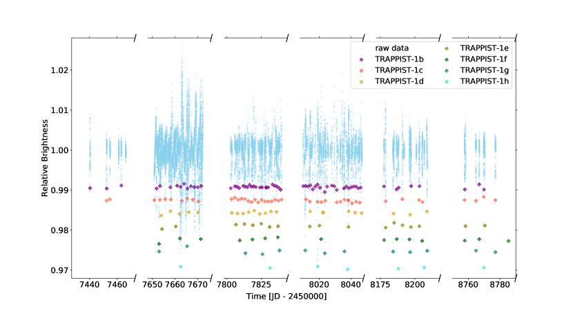
Figure 1: Spitzer photometric measurements (sky blue) resulting from observations of the star from February 2016 to Oct 2019 cleaned of data gaps between the four campaigns. Colored diamonds show the positions of the transits of the different planets with their corresponding depth + a constant offset by planet for clarity.

Back on the Spitzer dataset, we identified 29 blended transits (that is to say transits of multiple planets simultaneously) or partial transits (see Table 1) which were analyzed individually but not included in our global analysis presented in Section 3. Indeed, shapes of blended + partial transits are less constraining than well isolated full transits so we chose not to include them in our global analysis of all transits to have a better convergence. We also did not include them in our global planet by planet analyses for similar reasons when the transit was partial, and because we wished to deal with only one planet in these analyses.

Besides, we targeted 28 occultations of TRAPPIST-1b and 9 of TRAPPIST-1c with Spitzer/IRAC channel 2 with the aim to detect a signal or at least obtain an upper bound on the occultation depth and consequently derive the first empirical constraints on the planets’ thermal emission. Indeed, as the orbital planes of the seven TRAPPIST-1 planets are aligned to $<$ $0.3\deg$ at $90\%$ confidence (Luger et al., 2017b) their orbital tracks overlap over large fraction of their orbit Luger et al. (2017a), hence we expect all planets to undergo secondary ecplise. Given the small size of the planets, our best chance to catch an occultation signal is to phase-fold several occultations, which is why focusing on the inner planets (with the smallest periods) is the wisest choice. Furthermore, an updated TTV analysis using all transits observed by Spitzer, HST, K2, and ground-based transits observed up to 2019 (Agol et al., 2020) confirms that the expected eccentricities are very small (eccentricity ¡ 0.01 for all planets). In this context, we note that we did not spot any sign of planet-planet eclipses in our analyses of the blended transits, and for none of them was a planet “caught up” by a more inner one during its crossing of the stellar disk.

As described by Gillon et al. (2017), the star was observed nearly-continuously from 19 Sep to 10 Oct 2016 within the program 13067 (480hrs). The rest of the dataset (1061hrs) is composed of sequences of a few hrs corresponding to the observations of one or several transit(s) and/or occultation(s). For all observations in both bandpasses, each frame is composed of 64 subexposures each of 1.92 seconds on the target plus an additional 0.8s for read out, which gives a cadence of a point every 2.06 minutes.

Planet	# Isolated transits	# Blended or partial transits	Total
TRAPPIST-1 b	54	11	65
TRAPPIST-1 c	39	8	47
TRAPPIST-1 d	20	3	23
TRAPPIST-1 e	17	1	18
TRAPPIST-1 f	13	2	15
TRAPPIST-1 g	9	4	13
TRAPPIST-1 h	6	1	7

Table 1: Number of transits monitored by Spitzer from early 2016 to late 2019 for each TRAPPIST-1 planet

All these observations were obtained with the Infrared Array Camera (IRAC) (Carey et al., 2004) of the Spitzer Space telescope in subarray mode (32 $\times$ 32 pixels windowing of the detector) with an exposure time of 1.92 s. No dithering was used (continuous staring), and the observations were all done using the ‘peak-up’ mode (Ingalls et al., 2016) to maximize the accuracy in the position of the target on the detector’s sweet spot (as detailed in IRAC Instrument Handbook) to minimize the so-called ‘pixel phase effect’ of IRAC detectors (e.g., Knutson et al. 2008). All the data were calibrated with the Spitzer pipeline S19.2.0, and delivered as cubes of 64 subarray images of 32 $\times$ 32 pixels (pixel scale = 1.2 arcsec).

All 2016 and 2019 data were obtained with the 4.5 $\mu$m IRAC detector. In 2017 and 2018, additional observations were obtained at 3.6$\mu$m with the goal of further constraining the chromatic variability of the transit depths of the seven planets. The same method was used for the photometric extraction as that described by Gillon et al. (2017) and D2018. We converted the fluxes from MJy/sr to photon counts, and then we used the IRAF/DAOPHOT software (Stetson, 1987) to measure the flux of TRAPPIST-1 within a circular aperture of 2.3 pixels. For each subarray image, the aperture was centered on the star’s point-spread function (PSF) by fitting a 2D Gaussian profile, yielding measurements of the PSF width along the x- and y-axis in the process. We discarded subarray images corresponding to ¿ 10 $\sigma$ discrepant measurements for the PSF center, target flux, and background flux, as described by Gillon et al. (2014). We then combined the measurements per cube of 64 images. The photometric error of each cube (which is the standard error on the mean) was taken as the error of its average flux measurement.

2.2 Data analysis

Our data analysis was divided in three distinct steps. First, we performed individual analyses of each transit light curve to select an optimal photometric model and assess the variability of the photometry, see Section 2.2.1. We also carried out an analysis aiming to refine the stellar parameters of TRAPPIST-1, see Section 2.2.2. Then, we performed several sets of global analyses: (a) one with the entire set of transits to refine the physical parameters of the system; (b) seven others (one for each planet) for which we allow the transit depths to vary in order to assess their stability; and (c) a repeat of the seven global analyses (planet by planet), this time to improve the errors on the timings, see Section 2.2.3. Finally, we carried out a global analysis of the light curves from program 13175 (PI: L. Delrez) obtained around the expected occultation times for planet b and c to search for occultation signals, see Section 3.2 for details.

2.2.1 Individual analyses

We used our adaptive Markov-Chain Monte Carlo (MCMC) code (Gillon et al., 2010, 2012, 2014) to analyze each transit light curve individually (that is to say each individual transit). It uses the eclipse model of Mandel & Agol (2002) as a photometric time-series, multiplied by a baseline model to represent the other astrophysical and instrumental systematics that could produce photometric variations.

First, we select a model to represent each light curve through the minimization of the Bayesian Information Criteria (BIC; Schwarz 1978) which is given by the formula:

$$BIC=\chi^{2}+k\times log(N)$$ (1)

where $k$ is the number of free parameters of the model, $N$ is the number of data points, and $\chi^{2}$ is the best-fit chi-square. We tested a large range of baseline models to account for different types of external sources of flux variations/modulations (instrumental and stellar effects). This includes polynomials of variable orders in: PSF size and position on the detector (to account for the Spitzer ”pixel-phase” effect and the breathing of its PSF; Gillon et al. 2017); time (to correct for time dependent trends); and the logarithm of time (to represent the ”ramp” effect, Knutson et al. 2008). For some light curves the ”pixel-phase” effect was additionally corrected by complementing the position polynomial model with the bi-linearly-interpolated subpixel sensitivity (BLISS) mapping method presented by Stevenson et al. (2012). To do so, we sampled the detector area probed by the PSF center in several sub-pixel box such that at least five measurements fell within the same box. Further details of the implementation of BLISS mapping in our MCMC code can be found in Gillon et al. (2014). The details of the baseline model adopted for each transit light curve are given in Table LABEL:baseline_indiv. Once the baseline was chosen, we ran a preliminary analysis with one Markov chain of 50 000 steps to evaluate the need for re-scaling the photometric errors through the consideration of a potential under- or over-estimation of the white noise of each measurement and the presence of time-correlated (red) noise in the light curve. The white noise is represented by the factor $\beta_{w}$ issued from the comparison of the rms of the residuals and the mean photometric errors. The red noise is represented by the scaling factor $\beta_{r}$ derived from the rms of the binned and unbinned residuals for different binning intervals ranging from 5 to 120 min, following the procedure detailed in Winn et al. (2009). The values of $\beta_{w}$ and $\beta_{r}$ derived for each light curve are listed in Table LABEL:baseline_indiv.

The jump parameters that were randomly perturbed at each step of the Markov chains were:

• the mass $M_{\star}$, the radius $R_{\star}$, the effective temperature $T_{eff}$, and the metallicity [Fe/H] of the star, assuming the following prior probability distribution functions (PDFs) for these stellar parameters: $M_{\star}\in\mathcal{N}(0.089,0.007^{2})M_{\odot}$, $R_{\star}\in\mathcal{N}(0.121,0.003^{2})R_{\odot}$, $T_{eff}\in\mathcal{N}(2511,37^{2})$K and [Fe/H] $\in\mathcal{N}(0.04,0.08^{2})\mathrm{dex}$;

• the planet/star area ratio $dF=(\frac{R_{p}}{R_{\star}})^{2}$, where $R_{p}$ and $R_{\star}$ are the radius of the planet and the star, respectively;

• the transit impact parameter $b$ for the case of a circular orbit, defined as $b=a\mathrm{cos}(i_{p})/R_{\star}$ where $a$ and $i_{p}$ are, respectively, the semi-major axis and inclination of the orbit;

• the mid-transit time (inferior conjunction) for which we assumed a noninformative uniform prior PDF;

• the transit duration $T_{14}$, assuming a circular orbit (justified by really small eccentricities for all planets (Luger et al., 2017a, b; Agol et al., 2020)), defined as follow (Winn, 2010):

  $$T_{14}=\frac{P}{\pi}\arcsin\left[\frac{R_{\star}}{a}\frac{\sqrt{\big{(}1+\frac{R_{p}}{R_{\star}}\big{)}^{2}-b^{2}}}{\sin i}\right]$$ (2)

• the linear combinations of the quadratic limb darkening coefficients ($u_{1}$, $u_{2}$) in Spitzer’s 3.6 and 4.5 $\mu$m channels, defined as $c_{1}=2\times u_{1}+u_{2}$ and $c_{2}=u_{1}-2\times u_{2}$. Values and errors for $u_{1}$ and $u_{2}$ in a given band pass were interpolated from the tables of Claret et al. (2012, 2013) basing on the stellar parameters $T_{eff}$=2511 K $\pm$ 37 K, log$(g[\mathrm{cm\,sec^{-2}}])=5.18\pm 0.06$, and $[\mathrm{Fe/H}]=0.04\pm 0.08$ dex, (Delrez et al., 2018). The corresponding normal distributions were used as prior PDFs (for channel 1: $u1=\mathcal{N}(0.1633,0.0364^{2})$ and $u2=\mathcal{N}(0.2549,0.0570^{2})$, for channel 2: u1 = $\mathcal{N}(0.1442,0.0324^{2}))$ and $u2=\mathcal{N}(0.2173,0.0482^{2}))$ . In terms of combined limb darkening coefficients those value translates as: for channel 1: $c1=\mathcal{N}(0.5815,,0.0676^{2})$ and $c2=\mathcal{N}(-0.3465,0.0676^{2})$, for channel 2: c1 = $\mathcal{N}(0.5057,0.0581^{2}))$ and $c2=\mathcal{N}(-0.2904,0.05801^{2}))$.

All of our priors come from the updated system parameters presented in D2018. We recognize that those values were derived from analyses carried out on a subset of the same data set, noting that in this section our intention is not to determine the physical parameters of the system but rather to assess the stability (or variability) of the transits parameters. This subset is sufficient for this assessment.

We then re-scaled the photometric errors by multiplying the error bars by the correction factor $CF=\beta_{w}*\beta_{r}$. Once the correction factor was applied, we ran two Markov chains of 100 000 steps each to sample the PDFs of the parameters of the model and the system’s physical parameters (Ford, 2006), and assessed the convergence of the MCMC analysis with the Gelman & Rubin statistical test (Gelman & Rubin, 1992). Our threshold for convergence was a Gelman-Rubin statistic lower than 1.1 for every jump parameter, measured across the two chains.

For all of the analyses, the resulting values and error bars for the jump and system parameters as well as the complete details on the assumed baseline and on the correction factor applied can be found in Table LABEL:baseline_indiv. In addition to setting the baseline to use for each light curve, proceeding to individual analyses is also a way to search for variability in the transits, notably spot/faculae crossing or flares events (see 3.1.3).

2.2.2 Stellar parameters

1. Stellar parameters: In this paper, we derived stellar parameters using 142 of the 171 TRAPPIST-1’s planets transits observed with Spitzer (the transits not included were either partial or multiple). We proceeded as follows: first we inferred the density of the star $\rho_{\star}$ and its error through a global MCMC analysis of all stacked transit (detailed in the following paragraph). Then we derived the mass of the star $M_{\star}$ following the empirical relationship between $M_{K_{s}}$ (magnitude in K band) and $M_{\star}$ (with $M_{\star}$ spanning from 0.075$M_{\odot}$ ¡ $M_{\star}$ ¡ 0.70$M_{\odot}$) derived from 62 nearby binaries by Mann et al. (2019). The mass and its error were estimated by taking the metallicity of the star (from Van Grootel et al. (2018)) into account and through the use of the GitHub repository $M_{-}-M_{K}-$ provided by Mann et al. (2019), which accounts for systematic errors. With this estimate of the mass of the star and its error, we derived the radius of the star $R_{\star}$ from our posterior probability distribution function (PDF) on the density:

   $$R_{\star}=\Bigg{[}\frac{3M_{\star}}{4\pi\rho_{\star}}\Bigg{]}^{1/3}.$$ (3)

   Using the exquisite parallax value ($d=80.4512\pm 0.1211$ pc) from Gaia DR2 (Lindegren et al., 2018) and the integrated flux derived from Filippazzo et al. (2015), we computed the luminosity of the star, with no correction for extinction.:

   $$L_{\star}=4\pi d^{2}\int_{0\mu\mathrm{m}}^{1000\mu\mathrm{m}}F_{\lambda}(t)d\lambda,$$ (4)

   Finally, we derived the effective temperature of TRAPPIST-1 from its luminosity and its radius following the Stefan-Boltzmann Law:

   $$T_{eff,\star}=\Big{(}\frac{L_{\star}}{4\pi R_{\star}^{2}\sigma_{SB}}\Big{)}^{1/4},$$ (5)

   where $\sigma_{SB}$ is the Stefan-Boltzmann constant.

   We note that the computations of $L_{\star}$, $R_{\star}$ and $T_{eff}$ are straightforward, such that we don’t need to consider possible systematic errors. Their errors were then computed through error propagation on equations 3, 4 and 5.The stellar parameters derived from this approach are presented in Table 3.
   

   Quantity	Value
   Density $\rho_{\star}$ ($\rho_{\odot}$)	$52.31\pm 2.2$
   Mass $M_{\star}$ ($M_{\odot}$)	$0.0898\pm 0.0024$
   Radius $R_{\star}$ ($R_{\odot}$)	$0.1197\pm 0.0017$
   Luminosity $L_{\star}$ ($L_{\odot}$)	$0.000553\pm 0.000019$
   Effective temperature $(\mathrm{K})$	$2557\pm 47$

   Table 2: Updated stellar parameters of TRAPPIST-1 from the approach detailed in Section 2.2.2. 4.

2. Density inferred from individual planets:

   In the preceding paragraph we mentioned that we derived the stellar density through a global MCMC analysis of all stacked transit. This method uses the transits shapes and Kepler third’s law to constraint the stellar density (Seager & Mallen-Ornelas, 2003). However, in this particular case, the TRAPPIST-1 system is composed of 7 planets, that is to say 7 different sets of transit parameters. Hence, it is legitimate to investigate whether there are noticeable differences between the stellar density value inferred from each individual planet’s analysis and the one inferred from all transits together. The level of agreement between the two values would allow us to justify the use of the globally derived stellar density. Figure 2 shows the stellar density value as obtained from individual planet analysis with its error bars and a color code for the number of transits used in each analysis. Table 3 presents the corresponding values. In those analysis, for the star, $M_{\star}$, $R_{\star}$, $T_{eff,\star}$, [Fe/H], and the linear combinations c1 and c2 of the quadratic limb-darkening coefficients (u1,u2) for each bandpass were jump parameter, with informative priors on $M_{\star}$,$T_{eff,\star}$, [Fe/H], u1 and u2. And for each the planet, the transit depth 4.5$\mu m$, the impact parameter and the transit depth difference between Spitzer/IRAC 3.6$\mu m$ and Spitzer/IRAC 4.5$\mu m$ channels were jump parameters.

   Planet	# transits	$\rho_{\star}$ ($\rho{\odot}$)
   TRAPPIST-1 b	54	$44.6^{-3.9}_{+4.4}$
   TRAPPIST-1 c	39	$48.2^{-4.4}_{+3.7}$
   TRAPPIST-1 d	20	$46.5^{-12.0}_{+5.2}$
   TRAPPIST-1 e	17	$48.5^{-8.6}_{+5.8}$
   TRAPPIST-1 f	13	$57.3^{-7.2}_{+3.7}$
   TRAPPIST-1 g	9	$58.5^{-9.1}_{+6.0}$
   TRAPPIST-1 h	6	$53.8^{-18.0}_{+10.0}$

   Table 3: Stellar density from individual planets’s MCMC analyses with its $1-\sigma$ uncertainty. For each planets the number of transits used in the analysis is indicated in the second columns.

   
   

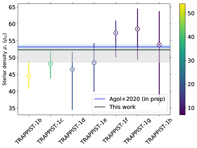
   Figure 2: Coloured dots gives the stellar density derived from MCMC analyses of transits from a single planet, solid black line gives the density derived from a global analysis of all transits observed with its $1-\sigma$ uncertainty in gray shades. Colorbar shows the number of transits used in each analysis. Solid blue line give the stellar density value computed by Agol et al. (2020) using a photodynamical model created with the mass-ratios and orbital parameters derived from a transit-timing analysis, with its $1-\sigma$ uncertainty in blue shades.

   From Figure 2, it appears that the inner planets prefer a lower stellar density than the outer ones. This could be translated as a correlation between period $P$ and the inferred stellar density $\rho_{\star}$. We carried out a linear regression between $\rho_{\star}$ and $P$, and computed the Akaike information criterion (AIC) and Bayesian information criterion (BIC) to identify the best fit, see Figure 3.

   

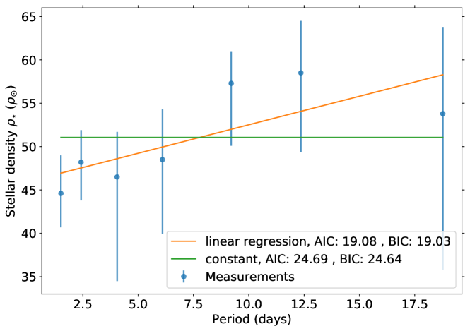
   Figure 3: Stellar density inferred from individual planet’s analysis versus period of the corresponding planet and its linear and constant fit with their corresponding AIC and BIC values.

   According to Figure 3, it turns out that a linear relation between the period and the stellar density is slightly preferred over a constant density (with a functional form of $\rho_{\star}=0.65*P+45.95$). This suggests that a correlation may exist between density and orbital period (and therefore b and $T_{14}$). However, the amplitude of this bias is smaller than the $1-\sigma$ error bars on the stellar density from the individual planet analyses, and therefore we conclude it is insignificant. On the origin of this weak trend in stellar density versus period, it could be the result of a trend of orbital eccentricity with orbital period. However, the eccentricities computed by Agol et al. (2020) do not seem to confirm this scenario. Another explanation could be that it is the consequence of an observational bias, as we have less transits for the outer planets (details on the number of transits per planets in Table 1). As a whole, this comparison shows the advantage of having a multiplanetary system where the planets sample different parts of the stellar disk. We conclude that using the stellar density derived from a global analysis of all transits, as we did in the previous paragraph, is appropriate.

   Furthermore, in Figure 2 we have added the stellar density computed by Agol et al. (2020) using a photodynamical model created with the mass-ratios and orbital parameters derived from a transit-timing analysis. We observe that the value derived from our global analysis is in excellent agreement with the one by Agol et al. (2020), which strengthens our confidence in using this value as the final one.

2.2.3 Global analyses

Once we selected a baseline model for each light curve (see Section 2.2.1), we continued to the next steps of our analysis. First, we carried out a global analysis of all the light curves together to refine the transit parameters. This is an update of the parameters presented in Table 1 of D2018 with the advantage that a global analysis with transits in both channels enables us to lift a part of the degeneracy between the transit parameters and the assumed limb-darkening coefficients. Second, we conducted 2*7 global analyses of transits for each planet to focus on computing first the transit timing variations and then the transit depth variations.

1. All light curves This analysis consisted of a preliminary run of one 50 000 step Markov chain to estimate the correction factors $CF$ that are applied to the photometric error bars (see Section 2.2.1) and a second run with two Markov chains of 500 000 steps for which we used the Gelman-Rubin test to assess the convergence. The relatively large number of steps for the two chains is necessary for a data set of this size. This method for analysis is identical to the one conducted by D2018, but includes an increased number of transits observed at 4.5 $\mu\mathrm{m}$ for all planets and newly observed transits at 3.6 $\mu\mathrm{m}$ for planets c, d ,e, f, g, and h. The jump parameters were $R_{\star}$, $M_{*}$, $T_{eff}$, [Fe/H], the linear combinations $c_{1}$ and $c_{2}$ of the quadratic limb-darkening coefficients ($u_{1}$, $u_{2}$) for each bandpass. For each planet, parameters include:
   - the transit depth at $4.5\mu\mathrm{m}$, $dF_{4.5\mu\mathrm{m}}$
   - the impact parameter, $b$
   - the transit depth difference between Spitzer/IRAC 3.6 $\mu\mathrm{m}$ and Spitzer/IRAC 4.5 $\mu\mathrm{m}$ channels, $ddF=dF_{3.6\mu\mathrm{m}}-dF_{4.5\mu\mathrm{m}}$
   - the transit timing variation (TTV) of each transit with respect to the mean transit ephemeris derived from the individual analyses
   

   For the mass of the star, we used a normal prior PDF based on the value derived in Section 2.2.2 ($M_{\star}$ = 0.0898 $\pm$ 0.0024 $M_{\odot}$). Then, for the metallicity and the limb-darkening coefficients in both channels we assumed the same normal prior PDFs as in Section 2.2.1. For the rest of the jump parameters, we assumed uniform noninformative prior distributions. We did not set the transit duration as a jump parameter because it is defined for each planet by its orbital period, transit depth, and impact parameter, combined with the stellar mass and radius (Seager & Mallen-Ornelas, 2003). Furthermore, dynamical models predict rather small amplitudes of variation for the transit durations (Luger et al., 2017a). The convergence of the chains was checked with the Gelman-Rubin statistic (Gelman & Rubin, 1992). The value of the statistic was less than 1.1 for every jump parameter, measured across the two chains, which indicates that the chains are converged. From the jump parameters the code deduced the physical parameters of the system at each step of the MCMC. In particular, the value of the effective temperature, $T_{eff}$, was derived at each MCMC step from the $R_{\star}$ and $L_{\star}$ values given in Section 2.2.2. Then, for each planet, values for the radius of the planet $R_{p}$, its semi-major axis $a$, its inclination $i$, its irradiation $S_{p}$, and its equilibrium temperature $T_{\mathrm{eq}}$ were deduced from the values for the stellar and transit parameters. Table 4 presents the outputs from this analysis.

   Parameters				Value
   Star				TRAPPIST-1
   Mass a  $M_{\star}$ ($M_{\odot}$)				$0.0898\pm 0.0023$
   Radius $R_{\star}$ ($R_{\odot}$)				$0.1234\pm 0.0033$
   Density $\rho_{\star}$ ($\rho_{\odot}$)				$47.98\pm 3.90$
   Luminosity a  $L_{\star}$ ($L_{\odot}$)				$0.000552\pm 0.000018$
   Effective temperature $(\mathrm{K})$				$2520\pm 39$
   Metallicity a  [Fe/H] $(\mathrm{dex})$				$0.0535\pm 0.088$
   LD coefficient, $u_{1,3.6\mu\mathrm{m}}$ a				$0.168\pm 0.016$
   LD coefficient, $u_{2,3.6\mu\mathrm{m}}$ a				$0.245\pm 0.019$
   LD coefficient, $u_{1,4.5\mu\mathrm{m}}$ a				$0.141\pm 0.016$
   LD coefficient, $u_{2,4.5\mu\mathrm{m}}$ a				$0.198\pm 0.018$
   Combined LD coefficient, $c_{1},3.6\mu m$				$0.581\pm 0.039$
   Combined LD coefficient, $c_{2},3.6\mu m$				$-0.322\pm 0.045$
   Combined LD coefficient, $c_{1},4.5\mu m$				$0.482\pm 0.031$
   Combined LD coefficient, $c_{2},4.5\mu m$				$-0.256\pm 0.044$
   Planets	b	c	d	e	f	g	h
   # of transits	54	39	20	17	13	9	6
   Period (days)	1.51088432 $\pm$ 0.00000015	2.42179346 $\pm$ 0.00000023	4.04978035 $\pm$ 0.00000266	6.09956479 $\pm$ 0.00000178	9.20659399 $\pm$ 0.00000212	12.3535557 $\pm$ 0.00000341	18.7672745 $\pm$ 0.00001876
   Mid-transit time $T_{0}$ - 2450000 ($\mathrm{BJD}_{\mathrm{TDB}}$)	7322.514193 $\pm$ 0.0000030	7282.8113871 $\pm$ 0.0000038	7670.1463014 $\pm$ 0.0000184	7660.3676621 $\pm$ 0.0000143	7671.3737299 $\pm$ 0.0000157	7665.3628439 $\pm$ 0.0000206	7662.5741486 $\pm$ 0.0000913
   Transit depth ($R_{p}^{2}/R_{\star}^{2}$) at $4.5\mu\mathrm{m}(\%)$	$0.7236\pm 0.0072$	$0.7027\pm 0.0068$	$0.3689\pm 0.0067$	$0.4936\pm 0.0081$	$0.6313\pm 0.0091$	$0.745\pm 0.011$	$0.351\pm 0.012$
   Transit depth ($R_{p}^{2}/R_{\star}^{2}$) at $3.6\mu\mathrm{m}(\%)$	$0.7209\pm 0.0067$	$0.721\pm 0.014$	$0.351\pm 0.016$	$0.491\pm 0.011$	$0.655\pm 0.019$	$0.724\pm 0.024$	$0.313\pm 0.027$
   Transit impact parameter $b$ ($R_{*}$)	$0.254^{+0.110}_{-0.085}$	$0.254^{+0.110}_{-0.087}$	$0.235^{+0.120}_{-0.094}$	$0.299^{+0.085}_{-0.072}$	$0.391\pm 0.056$	$0.430\pm 0.049$	$0.448\pm 0.054$
   Transit duration $T_{14}$ (min)	36.309 $\pm$ 0.093	42.42 $\pm$ 0.12	49.37 $\pm$ 0.32	56.31 $\pm$ 0.25	63.28 $\pm$ 0.31	69.10 $\pm$ 0.36	76.28 $\pm$ 0.81
   $R_{p}/R_{\star}$ at $4.5\mu\mathrm{m}$	$0.085062$ $\pm 0.000042$	$0.083827$ $\pm 0.000040$	$0.06073$ $\pm 0.00056$	$0.07025$ $\pm 0.00058$	$0.07945$ $\pm 0.00057$	$0.08632$ $\pm 0.0062$	$0.05927$ $\pm 0.0099$
   $R_{p}/R_{\star}$ at $3.6\mu\mathrm{m}$	$0.084903$ $\pm 0.00040$	$0.08495$ $\pm 0.00086$	$0.0593$ $\pm 0.0013$	$0.07009$ $\pm 0.00075$	$0.0809$ $\pm 0.0013$	$0.0851$ $\pm 0.0014$	$0.0559$ $\pm 0.0025$
   Inclination $i$ (∘)	$89.28\pm 0.32$	$89.47\pm 0.24$	$89.65\pm 0.15$	$89.663\pm 0.092$	$89.666\pm 0.059$	$89.698\pm 0.044$	$89.763\pm 0.037$
   Semi major axis a ($10^{-3}$AU)	$11.534_{-0.092}^{+0.099}$	$15.79_{-0.13}^{+0.14}$	$22.26_{-0.18}^{+0.19}$	$29.24_{-0.23}^{+0.25}$	$38.7740_{-0.31}^{+0.33}$	$46.81528_{-0.37}^{+0.40}$	$61.8656_{-0.49}^{+0.53}$
   Scale parameter $a/R_{\star}$	$20.13_{-0.55}^{+0.46}$	$27.57_{-0.76}^{+0.62}$	$38.85_{-1.1}^{+0.88}$	$51.0_{-1.4}^{+1.2}$	$67.1_{-1.9}^{+1.15}$	$81.7_{-2.3}^{+1.8}$	$107.9_{-3.0}^{+2.4}$
   Irradiation $S_{p}$ ($S_{\odot}$)	$4.15\pm 0.16$	$2.211\pm 0.085$	$1.114\pm 0.043$	$0.645\pm 0.025$	$0.373\pm 0.014$	$0.252\pm 0.0097$	$0.144\pm 0.0055$
   Equilibrium temperature $T_{\mathrm{eq}}$ (K)b	$397.6\pm 3.8$	$339.7\pm 3.3$	$286.2\pm 2.8$	$249.7\pm 2.4$	$217.7\pm 2.1$	$197.3\pm 1.9$	$171.7\pm 1.7$
   Radius $R_{p,3.6\mu m}$ ($R_{\oplus}$)	$1.1407\pm 0.035$	$1.141\pm 0.037$	$0.799\pm 0.026$	$0.944\pm 0.025$	$1.087\pm 0.027$	$1.147\pm 0.041$	$0.752\pm 0.037$
   Radius $R_{p,4.5\mu m}$ ($R_{\oplus}$)	$1.144\pm 0.027$	$1.128\pm 0.027$	$0.817\pm 0.022$	$0.945\pm 0.026$	$1.068\pm 0.028$	$1.161\pm 0.030$	$0.797\pm 0.025$

   • Informative prior PDFs were assumed for these stellar parameters

   • where $T_{eq}$ is computed from $T_{eq}=\Bigg{[}\frac{(1-A)*S_{p}}{4*\sigma}\Bigg{]}^{1/4}$, assuming a null Bond albedo

   Table 4: Updated system parameters: median values and 1-$\sigma$ limits of the posterior PDFs derived from our global MCMC analysis of all nonblended and partial transits of Trappist-1 planets observed by Spitzer.

   We note that prior to this paper different stellar parameters for TRAPPIST-1 were published. In 2019 Gonzales et al. (2019) presented a distance-calibrated SED of TRAPPIST-1 using a new NIR FIRE spectrum and parallax from the Gaia DR2 data release from which they derived updated fundamental parameters for the star. Back in 2018, Van Grootel et al. (2018) derived stellar parameters from two distinct approaches to compute the mass of the star, first via stellar evolution modeling, and second through an empirical derivation from dynamical masses of equivalently classified ultracool dwarfs in astrometric binaries. The stellar parameters we derived are in agreement with those from previous studies, as shown in Table 4.
   

   Quantity	Gonzales +2019	Van Grootel +2018	This paper
   Mass $M_{\star}$ ($M_{\odot}$)	0.0859 $\pm$ 0.0076	0.0889 $\pm$ 0.0060	$0.0898\pm 0.0023$
   Radius $R_{\star}$ ($R_{\odot}$)	0.1164 $\pm$ 0.0030	0.1182 $\pm$ 0.0029	$0.1234\pm 0.0033$
   Luminosity $L_{\star}$ ($L_{\odot}$)	0.000608 $\pm$ 0.000022	0.000522 $\pm$ 0.000019	$0.000552\pm 0.000018$
   Effective temperature $(\mathrm{K})$	2628 $\pm$ 42	2516 $\pm$ 41	$2520\pm 39$
   Parallax (mas)	80.45 $\pm$ 0.12	82.4 $\pm$ 0.8	80.45 $\pm$ 0.12

   Table 5: Comparison of stellar parameters value from various studies.

2. Planet by planet

   For each planet, the analysis itself was divided in three: a global analysis to extract the TTV of each transit, a global analysis with a free variation of the transit depth allowed to monitor its evolution with time, and finally an analysis of the occultation observations for planets b and c.

   1. Transit timing variations: We used nearly the same priors and jump parameters as in the individual analyses although we fixed the time of transit for epoch zero ($T_{0}$) and period $P$ for each planet, and set TTV as a jump parameter for each transit. The priors value for $T_{0}$ and $P$ are extracted from D2018. In this analysis, the same depth was assumed for all transits observed in the same bandpass. For each transit, we assumed the same baseline as the one obtained from its individual analysis.d Then, after one 50 000 step Markov chain, we re-scaled our photometric errors with the resulting correction factor and ran two Markov chains of 100 000 steps. Transits timings and their corresponding TTVs are reported in Table.LABEL:transit_timing_variations and displayed on Figure 4. From those, for each planet we performed a linear regression of the timings as a function of their epochs to derive an updated mean transit ephemeris, i.e., an updated value of the mid-transit time $T_{0}$ and the orbital period $P$ for each planet, see Table 4 (as done in D2018). Finally the median of the global MCMC posterior PDF of the transit depth in both channels are given in Table 6, those results are discussed in Section 3 and used to construct the planetary transmission spectra in Section 3.1.4.

      

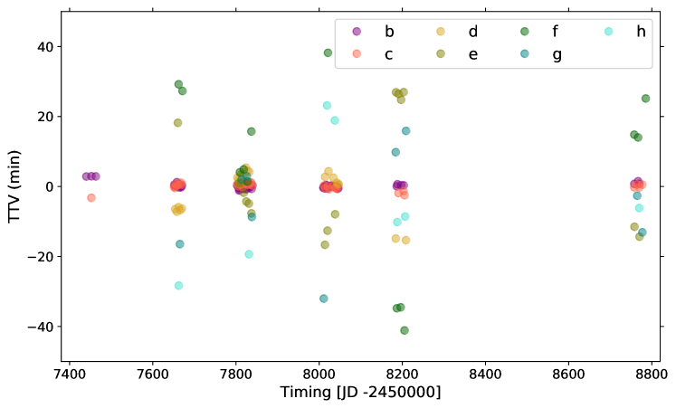
      Figure 4: TTVs measured for the seven planets as obtained from our global planet by planet analyses (see Section 2.2.3) relative to the ephemeris ($T_{0}$ and $P$) given in Table 4.

      Planet	Transit depth $dF_{3.6\mu\mathrm{m}}$ $\pm$ $1\sigma$ - $3\sigma$ (%)			Transit depth $dF_{4.5\mu\mathrm{m}}$ $\pm$ $1\sigma$ - $3\sigma$ (%)
      b	0.7179	0.0058	0.021	0.7195	0.0069	0.021
      c	0.7211	0.0130	0.039	0.6996	0.0058	0.018
      d	0.3407	0.0150	0.042	0.3653	0.0070	0.021
      e	0.4889	0.0010	0.027	0.4950	0.0075	0.023
      f	0.6463	0.0175	0.047	0.6240	0.0093	0.029
      g	0.7049	0.0330	0.094	0.7449	0.0110	0.024
      h	0.3120	0.0210	0.069	0.3478	0.0130	0.039

      Table 6: Median of the global MCMC posterior PDF of the transit depth derived from global analyses of all transits, planet by planet, with no transit depth variations allowed. Those values are used to construct transmission spectra in Section 3.1.4

   2. Transit depth variations: Here, we also used similar priors as in the individual analyses except that we fixed the values of transit timings and periods $P$ but for jump parameters we set the TTV of each transit and $\delta$dF, the depth variations from one transit to another. Again we ran first a 50 000 steps Markov chain to get the $CF$, and then two 100 000 steps chains. The evolution of the transit depths as a function of the epochs is presented for each planet in Figure 5. For further comparison, these figures also display the medians of the global MCMC PDFs as obtained by the previous global analysis with TTV and no $\delta$dF variations , values from Table 6. We compared the results obtained from the individual and global analyses of the transits and found them to be fully consistent. On Figure 5 we chose to plot the depth values obtained from the global analysis with $\delta$dF variations allowed instead of the individual analyses because the global analysis should be less impacted by systematic errors due to the red noise (i.e., the response of the pixels to time-varying illumination) in Spitzer photometry.
      

      

      

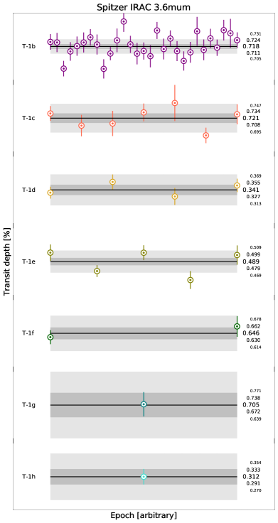
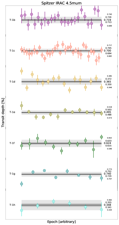
      Figure 5: Left: Evolution of the measured transit depths from the planet- per- planet global analyses of transit light curves at 3.6 $\mu\mathrm{m}$. The horizontal black lines show the medians of the global MCMC posterior PDFs from the planet- per- planet analyses with TTV and no transit depth variations allowed (with their 1$\sigma$ and 2$\sigma$ confidence intervals (see values in Table 6) in shades of gray) Events are ranked in order of capture, left to right (but not linearly in time). Right: Similarly, but for transits observed at 4.5 $\mu\mathrm{m}$.

   3. Occultations: We also used the eclipse model of Mandel & Agol (2002) to represent occultations of TRAPPIST-1b and c as photometric time-series, multiplied by a baseline model to represent external sources of photometric variations (either from astrophysical or instrumental mechanisms). The details of this analysis are given in Section 3.2, where we discuss the occultation observations and their interpretation. In this work, we analyzed 29 occultations of planet b and 8 occultations of planet c. All windows were observed in channel 2 ($4.5\mu\mathrm{m}$) as part of the DDT program 13175 (PI: L. Delrez). Our aim was to constrain the day-side brightness temperature of the two inner planets from the occultation depths. For both planets, we performed a global analysis of the occultation light curves, assuming as priors the Gaussian PDFs corresponding to the values for the stellar parameters and for the planets’ transit depths, impact parameters, mid-transit-times, and orbital periods derived from our global analysis of all Spitzer transit light curves (Table 4). Circular orbits were assumed for both planets, and the occultation depth was the only jump parameter of the analyses for which a uniform prior PDF $[0,+\infty)$ was assumed.We justify circular orbits assumption from the fact that in a system with planets that have migrated in Laplace resonances orbital, like TRAPPIST-1, eccentricity are expected to be very small. Indeed simulations carried out by Luger et al. (2017a) show that within a few Myr eccentricities of each planet damped to less than 0.01. In addition, recent results by Agol et al. (2020) from TTV and photodynamical model confirm that all planets eccentricities are most likely inferior to 0.01. Furthermore, when calculating the timing of secondary eclipse using the eccentricities given by Agol et al. (2020) and their $3-\sigma$ uncertainties we compute a shift in time of 0.28 hours and 0.27 hours for planet b and c respectively. Considering that the out-of-secondary eclipse time is $\simeq$ 2 hours for each light curve of this DDT program, we can confidently state that we did not miss the time of secondary eclipse. As with the transit analysis reported above, we identified the most applicable baseline for each light curve and ran a first chain of 50 000 steps to get the CF coefficients, applied these coefficients to the photometric error bars, and then ran two MCMC chains of 100 000 steps. We ascertained the convergence of our analyses with the Gelman & Rubin test (less than 1.1 for all jump parameters, as recommended by Brooks & Gelman (1998); Andrew Gelman (2003)). Unfortunately, no significant occultation signal was detected, Table 7 gives the occultation depth as output by the MCMC analysis with its 1 sigma and 3 sigma uncertainty. Those results are discussed in Section 3.2.

      Planet	$\delta_{occ}\pm 1\sigma$ (ppm)	$\delta_{occ}\pm 3\sigma$ (ppm)
      TRAPPIST-1 b	$90_{$-53$}^{+$59$}$	$90_{$-90$}^{+$180$}$
      TRAPPIST-1 c	$74_{$-52$}^{+$80$}$	$74_{$-74$}^{+$290$}$

      Table 7: Median of the occultation depths global MCMC posterior PDF + their 1$\sigma$ and 3$\sigma$ uncertainities as derived from the global analysis of 28 occultations of TRAPPIST-1b and 9 occultations of TRAPPIST-1c observed at 4.5 $\mu\mathrm{m}$.

3 Results and discussion

3.1 Transits

3.1.1 Mean transit ephemeris

Our global analysis of the transits of the seven planets led to an updated mean ephemeris, given in Table 4. The mean ephemeris for each planet was derived from a linear regression of the timings derived in Section 2.2.3 - planet by planet - as a function of their epochs. The new ephemerides are consistent with the ones derived in D2018. They do not take into account the TTVs, but should be sufficiently precise to forecast transit observations with an accuracy of better than $\sim$30 min (for the outer planets, and much better for the inner ones) within the next couple of years.

3.1.2 Noise floor

From the transit depths globally derived in each band (Table 6), and from the mean error on the depths of each transit given in Tables LABEL:global_3-6 and LABEL:global_4-5, we can estimate the amplitude of the noise floor of Spitzer transit monitoring of TRAPPIST-1. To do so, we compute the mean depth error $\overline{\mathcal{\sigma}_{dF,i,c}}$ for the $i$th planet in each band, $c$, from Tables LABEL:global_3-6 and LABEL:global_4-5. Assuming a purely white noise, the expected error for $n$ transits of planet $i$ in band $c$ should be $\sigma_{global,exp}=\frac{\overline{\mathcal{\sigma}_{dF,i,c}}}{\sqrt{n}}$. We then subtract in quadrature this expected value from the globally derived transit depth to estimate the Spitzer noise floor:

$$\sigma_{noisefloor}=\sqrt{\sigma_{global,obs}^{2}-\sigma_{global,exp}^{2}}.$$ (6)

From equation 6 we calculate the noise floor for each planet and derive the mean noise floor in each channel. The resulting values are 36 ppm in channel 1 and 22 ppm in channel 2. These values are consistent – and even lower actually– than those derived for a sample of $\sim$20 bright sun-like stars by Gillon et al. (2017). Considering how small these values are, we can conclude that stacking dozens of transits of TRAPPIST-1 observed in the infrared does improve the precision nearly in a $\sqrt{n}$ manner. This agrees well with the high photometric stabilty of TRAPPIST-1 observed during its Spitzer 20d continuous monitoring (Gillon et al., 2017; Delrez et al., 2018). Furthermore, the larger value of the noise floor at 3.6 $\mu$m –as observed by Gillon et al. (2017) for brighter Sun-like stars– suggests that this floor is mostly of instrumental origin, as the pixel-phase effect is significantly larger in IRAC channel 1 than in channel 2 and requires more complex baseline models (see Table A.1).

These results are particularly encouraging for the upcoming atmospheric characterization of the planets by transit transmission spectroscopy with JWST (Gillon et al., 2020). Indeed, the detectors of the JWST instruments (HgCdTe for all except SiAs for MIRI) should all have a much better intrapixel homogeneity than the IRAC InSb arrays, which should result in much less severe position-dependent effects in the JWST spectrophotometric light curves. This is supported by the results obtained by Kreidberg et al. (2014), who observed 15 transits of GJ1214b with HST/WFC3 (also an HgCdTe array, like NIRISS, NIRSPEC and NIRCAM) and obtained global transit depth errors consistent with a noise floor of $\sim 10$ ppm. Based on these considerations, noise floors in the 10-20ppm range can thus be expected for JWST observations of TRAPPIST-1, low enough to enable the detection and characterization of compact atmospheres around the planets (e.g., Lustig-Yaeger et al., 2019).

3.1.3 Time-dependent variations of the transit depths

One possible way to gain insight into the host star of a planetary system is to use transits as a scan of the stellar photosphere (Espinoza et al., 2018). By comparing the transit depths at different epochs we can identify unusual events that could inform us about the (in-)homogeneity of the star. Spot and faculae crossings are typically the kind of signatures detected with this method. For this purpose, we looked for unusually low or high depth values in the results from the global planet-by-planet analyses (Figure 5). We identified one clear outlier at $3\sigma$ lower than the other measurements for planet g (first point of the plot at 4.5 $\mu\mathrm{m}$ on Figure 5, epoch 0). The corresponding light curve and the fit for this epoch obtained from the global analysis are displayed in Figure 6.

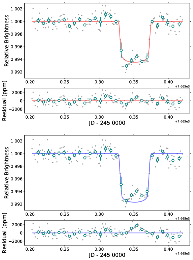
Figure 6: Top panel: Detrended light curve of the first isolated transit of TRAPPIST-1g observed by Spitzer with, superimposed in red, the best-fit model resulting from the global per-planet analysis with variations of the transit depth allowed. Bottom panel: Similar to Top panel but with the best-fit model resulting from the individual analysis assuming a constant depth for all transits superimposed in darkblue.

Yet, when we look at the same light curve as modeled in the global planet-by-planet analysis assuming a constant transit depth (Figure 6 Bottom panel), the first part of the transit seems to be consistent with the global model, while the rest is affected by a significant flux increase as expected for a spot-crossing event (Espinoza et al., 2018).

The discrepancy between individual and global fits is explained by the fact that in the global analyses per planet the model tries to optimize the fit with free transit depth variations allowed so the MCMC favor an unusually small depth for planet g to fit the unusual structure (see Figure 6). From the individual fit, Figure 6 bottom panel, we see that the structure in transit is very large (almost as long as the transit duration). If it corresponds to a spot crossing event the latter must be very large and at quite a low latitude as planet g has an impact parameter of $\simeq$ 0.42 from Table 4. To investigate the origin of this structure, first we checked all the planetary transits happening near the outlier, meaning several days before and several days after the event, and found no evidence of a similar structure in any of those transits including transits of TRAPPIST-1f, the planet with the closest impact parameter to planet g (see Table 4). Nevertheless, it is worth mentioning that the closest transit of planet h to the event (happening 3 days before the event at 2457662.55449 JD precisely) is one of the outliers shown in Figure 8 (see below for details of this Figure), yet this light curve is particularly noisy in- and out- of transit and therefore not reliable. Secondly, as this event was captured during the continuous observation of the system by Spitzer in 2016, we looked in the photometry for evidence of important variations in the amplitude of the stellar variability around this event as a sign of a sudden appearance of a massive spot that could explain the structure in planet g’s epoch 0 transit. To do so we applied a time rolling window (of fixed size equal to 20min) on the residuals of the detrended light curve corresponding to several days before and after the event, and from this rolling window we calculated the standard deviation and amplitude of the residual in order to catch any significant increase. Unfortunately, there does not seem to be any correlation between the appearance of the structure in the transit light curve of g and the variability of TRAPPIST-1, and as the Spitzer space telescope underwent some tracking problems during this campaign, our interpretation is limited. In a nutshell, this event is most probably isolated, which weakens the spot-crossing hypothesis considering that a massive photospheric heterogeneity would be needed to explain the observations. Nevertheless, as this structure cannot be corrected with any detrending of the systematics, one could still hypothesize that planet g transited with a different stellar hemisphere facing Earth than the other planets, or at least compared with f and h (as they have similar transit chords), and that the expected changes in stellar variability for such a large spot is not significant enough in the near infrared to significantly influence the stellar variability. However, this hypothesis is ruled out by the monotonic increase in the planets’ transit duration and impact parameters with orbital period, which implies an extremely coplanar planet system (Luger et al., 2017b).

Based on this experience with planet g, we visually inspected all individual light curves associated with the other outlier values in the global analysis results of Figure 5, but we did not find additional peculiar transits. To identify transit depth anomalies, we compute the median values and deviation of the photometric residuals in and out of transit (Table.LABEL:table_dev_res) as derived from the planet-by-planet global analyses (like in D2018). Figure 7 and Table LABEL:table_dev_res present the standard deviations obtained for the in- and out of transit residuals. Such statistics allow us to investigate the localized spot/faculae population through the ”in-transit” variations and the global stellar activity more generally through the ”out-of-transit” variations. We deal specifically with stellar flares in Section 3.3.

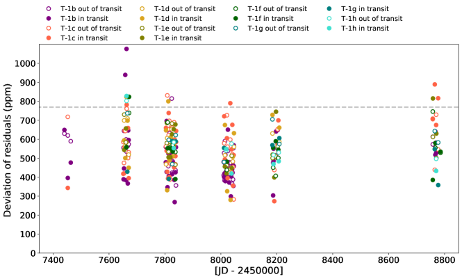
Figure 7: Standard deviation of the residuals (ppm) in- and out-of-transit for each planet (filled dots for in-transit data, empty dots for out-of-transit) such that for each transit’s epoch there is one empty dot and one filled dot. Each color is associated with a planet: purple for planet b, orange for c, yellow for d, olive for e, dark green for f, teal for g and turquoise for h. The dashed gray line show the limit value above we label the transits as outliers.

Considering the scatter of the measurements throughout the observations, we choose to define outliers as measurements whose standard deviations of the residuals is above 769ppm (median of deviation in- and out-of-transit + 3 $\sigma$, dashed gray line on Figure 7). Then, a careful look at all the light curves allows us to understand the source of uncertainty of those measurements. We were particularly interested in cases where the standard deviation of the in-transit residuals is larger than the standard deviation of the out-of-transit residuals as this could correspond to spot or faculae crossing events. Yet, we kept in mind that a the standard deviation of the residuals in-transit has a lower precision because it is calculated with fewer points than the standard deviation of out-of-transit residuals as the planets spend more time out-of-transit than in-transit, limiting the amount of data that can be collected in-transit. In Figure 7, we identify nine outliers, notably two transits of planet b which show a standard deviation of the in-transit residual of more than 1000ppm and 900 ppm respectively. The corresponding light curves are presented in Figure 8.

Figure 8: Transit light curves and their residuals for the 9 outliers identified on Figure 7. Each outlier was attributed a number in chronological order from 1 to 9, and the corresponding transiting planet at the time is indicated within the brackets.

In Figure 8, we observe that for some light curves the large value of the standard deviation of the in-transit residuals is explained by a structure that modifies the shapes of the transit. Such structures could indeed be due to the crossing of spots or faculae located within the transit chord of the planet at the time of transit. Light curves #1, #2, #4, #5, #6 and #9 could be interpreted as cases of bright spot crossing, while light curves #3, #7, and #8 could be interpreted as cases of dark spot crossing. The potential presence of spots could be worrisome for a precise derivation of the radius of the planets which is an essential step toward their detailed characterization (Roettenbacher & Kane, 2017). To weight the relevance of those anomalies and leverage the statistical bias mentioned above, we calculated the significance of the difference between the median residual in- and out-of-transit which we define by the following formula:

$$\mathrm{significance}=\frac{\absolutevalue{\mathrm{median}_{\mathrm{in}}-\mathrm{median}_{\mathrm{out}}}}{\sqrt{\sigma_{\mathrm{in}}^{2}+\sigma_{\mathrm{out}}^{2}}}$$ (7)

where $\mathrm{median}_{\mathrm{in}}$ and $\mathrm{median}_{\mathrm{out}}$ are the medians of the residuals in- and out-of- transit, and $\sigma_{\mathrm{in}}$ and $\sigma_{\mathrm{out}}$ are the absolute deviations of the residuals in- and out-of transit, respectively. The results are presented in Table.LABEL:table_dev_res and on Figure 9 for clarity.

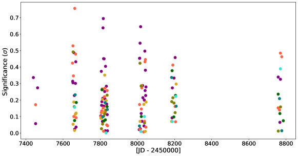
Figure 9: Significance of the difference between the median of the residuals (ppm) in and out of transit for each planet computed as: significance = $\frac{\absolutevalue{\mathrm{median}_{\mathrm{in}}-\mathrm{median}_{\mathrm{out}}}}{\sqrt{\sigma_{\mathrm{in}}^{2}+\sigma_{\mathrm{out}}^{2}}}$. Each dot stands for one unique transit. Each color is associated to a planet: purple for planet b, orange for c, yellow for d, olive for e, dark green for f, teal for g and turquoise for h.

We do not notice any significant difference between the in- and out-of-transit medians as they are comparable to within $1\sigma$ for all transits, see Figure 9. Those results do not favor the spot/faculae crossing hypothesis to explain the variability in transit depths that we discussed earlier, but rather systematic effects or some high-frequency stellar variability equally affecting in- and out-of-transit data to explain those anomalies. In fact, most of the outliers identified previously belong to the second of the five campaigns, during which the Spitzer telescope had some known drifting issues due to the use of inaccurate pointing coordinates (Gillon et al., 2017). We conclude that although it is hard to firmly discard this scenario, our results do not support the presence of stellar photospheric heterogeneities (spots and faculae affecting the transit shape at 3.6 $\mu\mathrm{m}$ and 4.5 $\mu\mathrm{m}$). However, one could argue that the lower contrast expected in the mid-IR may explain why we do not firmly detect any spot/faculae crossing event. Yet, recent results by Ducrot et al. (2018) failed to observe any spot crossing event in either the visible or the near-IR which favors a rather homogeneous stellar photosphere, at least for the portion transited by the seven planets. If numerous, spots would be expected to be relatively cool and small or out of the transits chords to agree with the very few events observed, see D2018, Ducrot et al. (2018), and Morris et al. (2018c). Nevertheless, it is still worth mentioning that some techniques are being developed to recover the true radii of planets transiting spotted stars with axisymmetric spot distributions from measurements of the ingress/egress duration, on the condition that the limb-darkening parameters are precisely known, see Morris et al. (2018b). The authors of the latter paper applied this technique to TRAPPIST-1 and concluded that active regions on the star seem small, low contrast, and/or uniformly distributed (Morris et al., 2018a). In any case, future JWST observations are expected to be more precise, less impacted by the limb darkening effect and therefore decisive for the confirmation of those conclusions, especially with an instrument like NIRSpec that will be able to cover a large spectral range (from 0.6 to 5.3 $\mu\mathrm{m}$, Ferruit et al. 2014).

Figure 10 shows the period-folded photometric measurements for all transits in both bands, corrected for the measured TTVs as well as the corresponding best-fit baseline models. We observe no recurrent structure for all planets. The limb darkening effect is less important at those wavelengths than in the visible or near-IR (see Ducrot et al. 2018) and the difference between the two channels is hardly noticeable by eye in Figure 10.

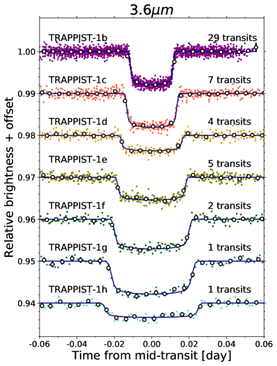
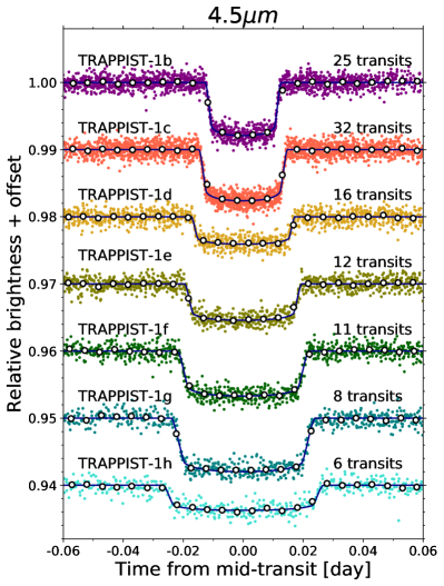
Figure 10: Left: Period-folded photometric measurements obtained with Spitzer/IRAC channel 1 (at 3.6 $\mu\mathrm{m}$) near the transits of the seven planets, corrected for the measured TTVs. Colored dots show the unbinned measurements; open circles depict the measurements binned over 5 minutes for visual clarity. The best-fit transit models are shown as dark blue lines. The numbers of transits that were observed to produce these combined curves are written on the plot. Right: Similarly at 4.5 $\mu\mathrm{m}$.

3.1.4 Transmission Spectra of the Planets

1. Stellar contamination
   As mentioned above, the TRAPPIST-1 planets are promising candidates for atmospheric characterization for several different reasons: the proximity of the system, the short periods of the planets, and their large sizes relative to their host. Yet, the host star itself might turn out to be an obstacle in characterizing the atmosphere of the planets if its photospheric inhomogeneity and evolution (formation, fading, and migration of spots/faculae) complicate the retrieval of atmospheric transmission signals. Consequently, a growing number of studies are dedicated to understanding the role played by the star’s activity and by the heterogeneity of its photosphere when studying exoplanets with the transit method (for studies of TRAPPIST-1, see Apai et al., 2018; Rackham et al., 2018; Zhang et al., 2018; Wakeford et al., 2018). To confirm the detection of atmospheric spectral features of terrestrial planets it is essential to optimize the disentanglement of signals of planetary and stellar origin. As stated before, intensive photometric follow up is an efficient way to probe the time-variable component of stellar activity of the host star. In the previous section we focused on the impact of the presence of stellar photospheric heterogeneities within the transits chords only. Here we discuss the potential impact of spectral contamination from out-of-transits spots & faculae on the chromatic variability of the transit depth through the transit light source effect (more details below) and how this can complicate the characterization of the planets. In particular, we construct the broadband transmission spectrum of each planet to estimate the amplitude of potential false spectral features introduced by star spots and faculae. In Figure 11, we show the updated version of the transmission spectra of the seven planets presented by Burdanov et al. (2019). This update consists of an additional point at $3.6\mu\mathrm{m}$ for planets c-h, updated values at $4.5\mu\mathrm{m}$, and updated weighted mean values for all planets (continuous lines in the plot). Figure 11 combines results from de Wit et al. (2016, 2018); Ducrot et al. (2018); Wakeford et al. (2018); Burdanov et al. (2019) and shows transmission spectra with the largest number of experimental measurements to date for the TRAPPIST-1 planets. We have decided not to include HST measurements (de Wit et al., 2016, 2018; Wakeford et al., 2018) to compute the weighted mean depth for each planet (black continuous line). This choice is justified by the fact that, although the transit transmission spectra measured in HST/WFC3 spectra are certainly reliable in relative terms, the derived absolute value of the transit depths themselves can be questioned because HST/WFC3 spectrophotometric observations are affected by orbit-dependent systematic effects which can result in diluted or amplified monochromatic transit depths, as implied by several previous studies (de Wit et al., 2016; Wakeford et al., 2018; Ducrot et al., 2018).

   

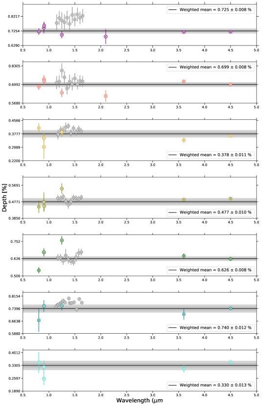
   Figure 11: Updated version of the transit transmission spectra of the seven TRAPPIST-1 planets. In each subplot the continuous line is the weighted mean depth $\overline{\Delta f}$ of all non-HST measurements, with its 1$\sigma$ and 2$\sigma$ confidence intervals, in shades of gray calculated from the following formula $\sigma_{\overline{\Delta f}}=\frac{1}{\sum w_{i}}\sqrt{\sum(w_{i}\sigma_{i})^{2}}$, $\sigma_{i}$ and $w_{i}$ being respectively the error of measure i and its weight (i.e number of transits observed at each wavelength). HST measurements are presented as gray points. Coloured dots stand for the measured transit depth at the effective wavelength of the instrument, ground based measurement are symbolized by circles and space based measurement by hexagons. Each point is associated with a particular observation, in ascending order of wavelength: one point for K2 (value from Ducrot et al. (2018)), one for SSO (value from Ducrot et al. (2018)), one for LT (value from Ducrot et al. (2018)), one in the J-band for UKIRT/WFCAM and/or AAT (value from Burdanov et al. (2019)), one for the NB-2090 filter band, one point for VLT/HAWK-I only for planet b and c (value from Burdanov et al. (2019)), in IR 11 points for b and c, 10 for d, e, f and 13 for g taken with HST/WFC3 (values from de Wit et al. (2016, 2018); Wakeford et al. (2018)) and two points for Spitzer/IRAC channel 1 and 2 (values from this work, Table 6).

   Concerning the Spitzer observations only, in Figure 11 we observe that for all planets there are no significant differences between the $3.6\mu\mathrm{m}$ to $4.5\mu\mathrm{m}$ measurements (particularly in comparison with visible and near-IR variations), both agreeing with each other better than 2-$\sigma$ for all planets (value given in Table 6). When we next consider all of the observational points, the depths measured at different wavelengths are all consistent with each other at better than 1-$\sigma$ for planet b, and better than 2-$\sigma$ for planets d and g. However, for planets c, e, f, and h the transmission spectra show a scatter larger than expected based on the measurement errors alone. For planet h, only one point exceeds the two sigma confidence, the one derived from the Liverpool Telescope (LT) dataset. But, it is worth mentioning that the effective wavelength for LT observations ($0.9046$ $\mu\mathrm{m}$) is very close to that of SPECULOOS ($0.9102$ $\mu\mathrm{m}$) and yet the SPECULOOS value is not discrepant with the others. Furthermore those data were obtained at the same period on SPECULOOS and LT. Therefore, the difference in depth measurements between those two facilities is probably more of a systematic rather than a physical origin. Yet, for planet c and e, the points that are the most inconsistent with the weighted mean value are the measurements obtained from observations carried out in the near-Infrared, with either UKIRT, VLT, AAT, or HST. Such spectroscopic transit depth variations could be the result of photospheric heterogeneity on the host star, such as unocculted active regions, which could alter the observed transit depths through the transit light source effect (Rackham et al., 2018). This effect refers to the case where a difference between the disk-averaged spectrum and the spectrum of the transit chord - which is the actual light source from the measurement - imprints spectral features on the observed transmission spectrum (Rackham et al., 2019). In that regard, Zhang et al. (2018) modeled the transit light source effect by adapting spots parameters to fit the empirical transit depth of the TRAPPIST-1 planets derived from K2, SPECULOOS, LT, HST, and previous Spitzer observations (Ducrot et al. 2018, de Wit et al. 2016, 2018; Wakeford et al. 2018, D2018). The new depths that we derived at $3.6\mu\mathrm{m}$ for planets c, d, e, f, g and the updated value at $4.5\mu\mathrm{m}$ for all planets allow us to compare two new observational values with the theoretical predictions of Zhang et al. (2018). Figure 12 shows the combined transmission spectrum for b+c+d+e+f+g+h and best-fitting contamination model formerly computed by Zhang et al. (2018) using K2+SSO+HST+Spitzer (IRAC channel2, D2018 ). We computed the $\chi^{2}$ statistic value of the best-fit contamination model published in Zhang et al. (2018) to our observational points (that contains updated and new points compared to the values used in Zhang et al. (2018)). We obtain a $\chi^{2}$ of 17.5 with a p-value (Pearson, 1900) of $0.29$, indicating that the model is not ruled out by the data. The next step would be to see if those new data points could be better fitted with a new run of the model presented by Zhang et al. (2018) or with any other model, but this is out of the scope of this paper.

   

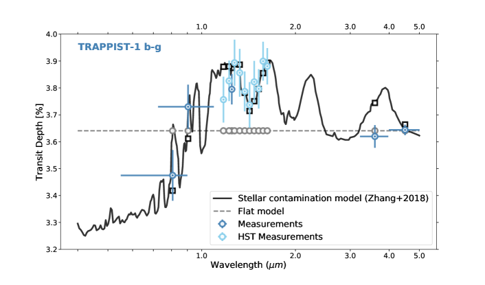
   Figure 12: TRAPPIST-1 combined transmission spectra for planets b+c+d+e+f+g (blue points) constructed from individual spectra (see Figure 11), over-plotted with the stellar contamination model (black solid line) derived by Zhang et al. (2018) from the fit of previously published K2 + SPECULOOS-South (Ducrot et al. 2018) + HST (de Wit et al. 2016, 2018; Wakeford et al. 2018) + Spitzer (D2018) data. The black squares are the integrated depth values as predicted by the stellar contamination model of Zhang et al. (2018) in each spectral band for which observations were performed, and gray dashed lines is the flat model at the weighted mean value of the transit depth. Wavelength is in log scale.

   Based on their analysis, Zhang et al. (2018) concluded that TRAPPIST-1 should be covered at $\simeq 50\%$ with spots and $\simeq 40\%$ with faculae overall. Yet, their model predicted some location-dependent spot covering fraction over the star. For instance it favored a scenario where the region transited by the planets was less spotted than the whole disk, with a spot covering fraction of only $\simeq$ 10% of the transit chord. The authors interpreted this mismatch as the presence of an active region left unprobed by the transit chords, such as an active high-latitude or circumpolar spot. Similar structures had already been observed on fully convective M-dwarfs (Barnes et al., 2015, 2017). In light of the previous section which showed that neither our work nor D2018 nor Ducrot et al. (2018) detected clear spot/faculae crossing events, while the transit chords represent 56% of the hemisphere (D2018), and considering the results of Zhang et al. (2018), it could indeed be possible that spots appear at preferential latitudes, like the poles. As mentioned by Zhang et al. (2018), one way to confirm this could be to use Doppler tomography with the upcoming E-ELT/HIRES instrument, as has already been done for a few brighter stars (Barnes et al., 2005), or to use spectral template fitting to constrain spot sizes and population through molecular band observations (Vogt, 1979). Meanwhile, analyses driven by Morris et al. (2018c) on the Spitzer dataset (observations carried out from 2016 up to 2017) using the self-contamination method from Morris et al. (2018b) suggest that the mean photosphere of TRAPPIST-1 was rather similar to the photosphere occulted by the planets, even if they could not rule out a scenario of small-scale magnetic activity analogous in size to the smallest sunspots present within (or outside) of the transit chords. Such a scenario could also agree with our empirical results but cannot be confirmed with the current photometric precision of the existing instruments. Last, it is important to mention that a method to separate the planetary transmission spectrum from stellar molecular features using the out-of-transit stellar spectra, planetary transit geometries, and planetary atmospheric models has been developed by Wakeford et al. (2018). After discarding several scenarios, Wakeford et al. (2018) concluded that a three component flux model composed of the photosphere, hotter spots ($\simeq$ 35%) and some faculae (¡3%), with an additional small fraction of flux (1%) from magnetic activity would be the most likely scenario for TRAPPIST-1, and that the planetary transmission spectra were likely not contaminated by any stellar spectral features (Wakeford et al., 2018).
   

   Considering next the transit spectra of planets c and e, it should be emphasized that, as mentioned in section 3.1.3, de Wit et al. (2016, 2018) warned us that HST/WFC3 spectrophotometric observations are affected by orbit-dependent systematic effects, which can alter the monochromatic absolute transit depth values. Furthermore, concerning the measurements obtained from UKIRT, VLT and AAT, Burdanov et al. (2019) highlighted a few data gaps during some observations that could have influenced the derived transit depth values, and also emphasized how strong the influence of water vapor can be at those wavelengths for ground-based observations. Finally, those observations are also the least numerous ones, with less than 3 combined transits for all planets used to derive the values plotted in Figure 11 in the corresponding bands. For these reasons, it is important to remain cautious about the relevance of our interpretation of planet c and e transmission spectra. For planet f, however, it is different as the dispersion of the measurements is even larger, with clear outliers in J band and in the visible. On one side, we could again argue for low statistics in the near-IR band to justify the large gap between UKIRT measurement and the weighted mean value, as only 3 transits were used to compute this value. But in the visible, K2’s surprisingly low depth value seems more robust as it was derived from the combined analysis of 6 transits. The transmission spectrum of planet f is really intriguing and more observations in the near-IR and visible are required to draw proper conclusions on the origin of its larger scatter.

   All things considered, we can confidently state that the observed transmission spectra of the TRAPPIST-1 planets are not flat, but we cannot conclude on weather those variations could be attributed to stellar contamination or low statistic data. Nonetheless, these Spitzer observations provide unique statistics and show no discrepancy greater than $400$ ppm peak-to-peak and consistency at better than 2-$\sigma$ for all planets. Recent papers are converging toward a three spectral component TRAPPIST-1 photosphere as the most likely scenario (Rackham et al., 2018; Zhang et al., 2018; Wakeford et al., 2018), and authors are proposing different approaches to constrain this stellar photosphere, such as: time resolved spectral decomposition (Gully-Santiago et al., 2017); joint retrievals of stellar and planetary properties (Pinhas et al., 2018); visual transmission spectroscopy (Rackham et al., 2017); transit-crossing events (Espinoza et al., 2018); or the use of out-of-transit stellar spectra to reconstruct the stellar flux (Wakeford et al., 2018). The combination of multiple approaches toward the study of the star’s photosphere represents a promising path toward the disentangling of the planetary atmospheric features from the stellar signals and therefore the optimization of future transit transmission spectroscopy with the eagerly-awaited JWST.
   

2. Comparison with atmospheric models
   One of the most ambitious results that the exoplanet community wishes to achieve with the upcoming JWST is the first detection of an atmosphere around a terrestrial exoplanet (Madhusudhan, 2019). For the reasons discussed earlier, the TRAPPIST-1 system is particularly favorable for the achievement of this goal via transit transmission spectroscopy (Barstow & Irwin, 2016; Morley et al., 2017; Batalha et al., 2018; Krissansen-Totton et al., 2018; Lustig-Yaeger et al., 2019; Fauchez et al., 2019), and offers the opportunity to probe atmospheres not only around terrestrial planets but also around temperate terrestrial planets within the habitable-zone of their host star. In the previous section, we discussed the impact of stellar contamination on the planet transmission spectra, and we concluded that several solutions are being developed to optimize the retrieval of planetary atmosphere features. In this section, we do not consider stellar contamination and only discuss potential detections of atmospheric features of the TRAPPIST-1 planets. Here, we limit our discussion to include only the cases of TRAPPIST-1b, c, e and g because (a) b and c have the smallest periods - that is to say the most transits and therefore the greatest precision on measurements, (b) planet e is arguably the most promising candidate for habitability, for the reasons given in Wolf (2017, 2018), Turbet et al. (2018) and Fauchez et al. (2019), and (c) planet g was the most observed with HST/WFC3 (Wakeford et al., 2018).

   Combining ground and space-based observations, we can construct the broadband transmission spectra obtained in various wavelengths for each planet and compare them to recent atmospheric models of the TRAPPIST-1 atmospheres computed by Lincowski et al. (2018), see Figure 13. To construct this figure, we have added a vertical offset to Lincowski et al. (2018)’s models to optimally overlap the observations. These offsets correspond physically to the difference between the assumed radius for TRAPPIST-1b and the solid body radius assuming a model atmosphere and its associated absorbing radius above the surface (Lincowski et al., 2018). We have applied this offset such that the models crossed the measured transit depth at the value of the sum of the weighted mean depth of each planet (shown in black solid line on Figure 11). For the reasons mentioned above we also applied an offset to adjust the mean level of each HST/WFC3 spectra to the weighted mean depth for each planet. By doing this we can benefit from the trustful information given by HST/WFC3 measurements on relative depths and use it to better constrain atmospheric properties.

   

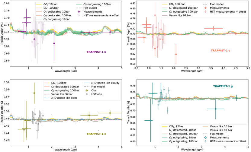
   Figure 13: Top-left: Transit transmission spectrum of TRAPPIST-1b from observations (similar Figure 11, except for HST-measurement on which an offset has been applied) compared with simulated transit transmission spectra derived by Lincowski et al. (2018) for different terrestrial atmospheres. Each color is associated with a different scenario: - gold stands for 10 or 100 bars $\mathrm{CO}_{2}$-rich atmospheres - salmon stands for 10 or 100 bars $O_{2}$-rich desiccated atmospheres - green stands for 10 or 100 bars $O_{2}$-rich outgazing atmospheres - brown stands for 10 or 92 bars Venus-like atmospheres - and blue stands for an aqua planet with either clear or cloudy sky. Top-right: Similarly but for TRAPPIST-1c. Bottom-left: Similarly but for TRAPPIST-1e. Bottom-right: Similarly but for TRAPPIST-1g.

   Those spectra illustrate our current knowledge of the transit transmission spectra gained from follow-up observations. The wavelength range that has been probed since the discovery of the system goes from $\simeq$ 0.6 $\mu\mathrm{m}$ to $\simeq$ 5 $\mu\mathrm{m}$. In this spectral range the strongest molecular features that we could expect in the absence of clouds and haze - and in a plausible planetary environment - are $\mathrm{CO}_{2}$, $\mathrm{CH}_{4}$, $\mathrm{H}_{2}\mathrm{O}$ and $\mathrm{CO}$ (Tennyson & Yurchenko, 2012; Gordon et al., 2017; Morley et al., 2017). Considering the distribution of the effective wavelength of the different instruments we can only look for some localized, strong features: - the $\mathrm{CO}_{2}$ 4.3 $\mu\mathrm{m}$ spectral feature in the 4-5 $\mu\mathrm{m}$ channel of Spitzer/IRAC (width of the bandpass is 1.015 $\mu\mathrm{m}$ for that channel) - the $\mathrm{CO}_{2}$ 2.1 $\mu\mathrm{m}$ spectral feature in the VLT/HAWK-I’s NB-2090 filter bandpass (width of the bandpass is 0.020 $\mu\mathrm{m}$ for NB-2090 filter) - and the $\mathrm{CH}_{4}$ 3.3 $\mu$m spectral feature in the 3.15-3.9 $\mu\mathrm{m}$ channel of Spitzer/IRAC (width of the bandpass is 0.750 $\mu\mathrm{m}$ for that channel).

   We deliberately did not consider models of hydrogen-dominated atmospheres as there is now plenty of evidence that all TRAPPIST-1 planets are unlikely to host this kind of atmospheres. First, transmission spectroscopy with HST/WFC3 has shown that most of the planets in the system are unlikely to have cloud-free H2-rich atmospheres (de Wit et al., 2016, 2018; Wakeford et al., 2018). Although transmission spectroscopy cannot rule out H2-dominated atmospheres containing high-altitude aerosols (Moran et al., 2018), such configuration is in fact unlikely. This stems from the fact that any small variation of hydrogen content between planets, as expected from (1) variations in the hydrogen-rich gas accretion rates during the planet formation phase (Hori & Ogihara, 2020) and from (2) variations in H2 escape rates (Owen & Mohanty, 2016; Bolmont et al., 2017; Bourrier et al., 2017), are expected to produce large variations in density between planets (Turbet et al., 2020) that are not observed (Grimm et al., 2018; Agol et al., 2020).

   The transmission spectrum of TRAPPIST-1b - HST/WFC3 measurements excluded - can be relatively well fit by the models. It contains the observational points with the best precision with an error bar as low as 58 ppm (Table 6) in Spitzer/IRAC channel 2 measurement (thanks to the combination of 28 transits). Yet, even with 28 transits combined the precision reached is still of same order as the expected amplitude for detectable atmospheric features on TRAPPIST-1b ($\simeq 100\%$ (Morley et al., 2017; Lustig-Yaeger et al., 2019). TRAPPIST-1c’s spectrum shows a greater scatter than the one of b with an apparently poor fit to the models, yet the uncertainties on the measurements are large (at least relatively to the expected atmospheric features) and those variations are not significant at more than 3-$\sigma$. Then, for planets e and g, the expected spectral features are even shallower than for b and c, and the observations are less precise because of the smaller number of transits analyzed; thus it is impossible to speculate on the presence of any molecular species.

   One possibility to gain some precision in the measured transit depths is to study the combined transit transmission spectrum of several planets. Figure 14 shows a transmission spectrum constructed from the combination of planets b, c, d, e, f and g’s transmission spectra.

   

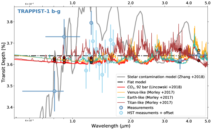
   Figure 14: Similar to Figure 12 with simulated combined transmission spectra. Observations and their error bars are in blue. Simulated combined transit transmission spectra expected for $\mathrm{CO}_{2}$ dominated atmospheres is in red, for Earth-like atmospheres in blue-green, for Venus-like atmospheres in orange and for Titan-like atmospheres in brown. Corresponding coloured hexagons give the value expected from the models at the wavelengths of the observations. Wavelength is in log scale.

   This figure is similar to Figure 12 , except from the fact that we have now put an offset on HST-measurements to adjust the mean level to the weighted mean depth calculated from the rest of the observations, and the have over-plotted several simulated combined transmission spectra from Lincowski et al. (2018) and Morley et al. (2017). For the reasons we mentioned earlier, we have added a vertical offset to the atmospheric models to optimally overlap the observations. The offset value is such that the models crossed the value of the sum of the weigthed mean depth of each planet (shown in black dotted line on Figure 12). From the observations, only points derived from the Spitzer dataset analyses have a precision of comparable magnitude than the variations expected in presence of an atmosphere. Table 8 gives the reduced chi square $\chi^{2}_{\nu}=\chi^{2}/\nu$ for each model if its aim was to fit the observations, with $\nu$ the number of degrees of freedom and $\chi^{2}$ is defined by:

   $$\chi^{2}={\sum_{i}}\frac{\big{(}pred(i)-obs(i)\big{)}^{2}}{\sigma(i)^{2}}$$ (8)

   where $obs(i)$ is the measured depth at wavelength i, $\sigma(i)$ its error, and $pred(i)$ is the depth predicted by the model for wavelength i.

   Model fitted to the data	Reduced $\chi^{2}$
   No atmosphere	1.1920
   Venus-like atmosphere c	1.4376
   $CO_{2}$, 92bar b	1.5086
   Earth-like atmosphere c	1.5554
   Titan-like atmosphere c	1.8542

   • Zhang et al. (2018)

   • Lincowski et al. (2018)

   • Morley et al. (2017)

   Table 8: Reduced $\chi^{2}$ values for different atmospheric models. The number of degrees of freedom used in calculating the reduced-chi-squared values listed here equal to the size of the observation sample - 1.

   On Figure 14, Earth-like (Morley et al., 2017), Venus-like (Morley et al., 2017) and $\mathrm{CO}_{2}$-dominated (Lincowski et al., 2018) atmospheric scenarios seem to agree reasonably well with Spitzer experimental values, showing notably a larger depth in IRAC channel 2 than in channel 1 like the data suggest. In contrast, in a Titan-like (i.e., CH₄-dominated) scenario the depth measured in channel 1 is expected to be larger than the one measured in channel 2. This explains by the fact that a Titan-like atmospheres exhibit a strong, broad CH₄ absorption feature centered at 3.3$\mu$m that produces a deeper transit depth in the Spitzer channel 1 than in the channel 2. We note that the discrepancy between Titan-like atmospheres and the measured Spitzer channels 1-2 transit depths would be even greater if we assume that stellar contamination occurs at these wavelengths. Looking at the value reported in Table 8 we indeed confirm that a Titan like atmosphere appears to be the less likely considering our current observational points and their errors bars. As a very preliminary estimation, we could predict that, assuming high-mean-molecular weight atmospheres the TRAPPIST-1 planets, it is rather unlikely that most of the TRAPPIST-1 planets possess a $\mathrm{CH}_{4}$-dominated atmosphere.

   Yet, what we can also note from Table 8 is that the most likely scenario, given the current observations, is a model with no atmosphere where the transit depth is equal to the sum of the weighted mean depth at all wavelengths. However, we cannot drawn any clear conclusion because as we mention before we are extremely limited by the precision on our each measurements, even for Spitzer/IRAC channel 1 and 2.

   In conclusion, from Figure 13 we can only lament that our current level of precision is unfortunately not high enough to draw proper conclusions about the existence of compact, high mean-molecular weight atmospheres around the TRAPPIST-1 planets. Even the combination of 22 transits of planet b at 4.5 $\mu\mathrm{m}$ and 28 transits at 3.6 $\mu\mathrm{m}$ with the Spitzer space telescope cannot reduce our error bars to sufficient precision. Nevertheless, the combined transmission spectrum of planets b to g presented in Figure 14 tells us that the atmospheres of the TRAPPIST-1 planets are unlikely to be methane-dominated. Yet, this interpretation is made from only two observational points (Spitzer IRAC channels 1 and 2) and requires further investigation. A more rigorous study of the planets’ atmospheres will likely have to wait for JWST. In particular, the Prism mode of the NIRSPEC instrument shows a high potential to detect compact atmospheres around the planets (Batalha et al., 2018; Lincowski et al., 2018; Lustig-Yaeger et al., 2019; Lincowski et al., 2019; Fauchez et al., 2019). Several independent simulations predict that it could take less than 10 transits for the seven planets to detect the dominant absorber (Morley et al., 2017; Krissansen-Totton et al., 2018; Lustig-Yaeger et al., 2019; Wunderlich et al., 2019; Batalha et al., 2018). This number may increase if clouds and/or photochemical hazes are present (Fauchez et al., 2019). Moreover, more and more studies focus on understanding how JWST could provide us with insight into the planets’ potential habitability, either through the presence of biogenic oxygen in their atmospheres (Lincowski et al., 2018; Morley et al., 2017; Meadows et al., 2018), or via the detection of anoxic biosignatures such as $\mathrm{CH}_{4}$ + $\mathrm{CO}_{2}$ minus $\mathrm{CO}$ (Krissansen-Totton et al., 2018), while keeping in mind the importance of false positives/negatives (Harman et al., 2015; Reinhard et al., 2017).

3.1.5 Transit timing variations

While the near-infrared (nIR) spectropolarimeter / velocimeter for the Canada-France-Hawaii Telescope (CFHT) SPIRou (Donati et al., 2018) is expected to soon provide us with the first radial velocity detection of the TRAPPIST-1 planets (Klein & Donati, 2019), transit timing variations (TTVs) are still the most useful tool for precisely estimating the masses of the planets. Combining the measured sizes (from transits) and masses (from TTVs) of the planets, we can deduce their densities and draw some inferences about their bulk compositions (Grimm et al., 2018; Dorn et al., 2018; Turbet et al., 2019). Furthermore, TTVs allow us to comprehend the complex dynamics that exists between those seven fast orbiting planets. Our measured timings as obtained from the global analysis (planet-by-planet) are presented in Table LABEL:transit_timing_variations, and will be used in a subsequent paper to improve the determination of the masses of the planets through the TTV method. For any future use of the transit timings of the TRAPPIST-1 planets from Spitzer observations, we recommend to use the ones derived from the global analyses planet by planet rather than from individual analysis as they are less impacted by systematic errors due to the red noise.

3.2 Occultations

In this work, we analyzed 29 predicted occultations of planet b and 8 predicted occultations of planet c, all observed in channel 2 (centered in $4.5\mu\mathrm{m}$), hereafter indexed as c2. Our aim was to derive the dayside brightness temperature $T_{p,c2}$ of the two inner planets from their occultation depths. Unfortunately, we did not detect the occultation signal of either planet b or planet c (see Figure 15), but we were able to estimate a $3-\sigma$ upper limit on their dayside brightness temperatures. No occultation observations were taken in channel 1.

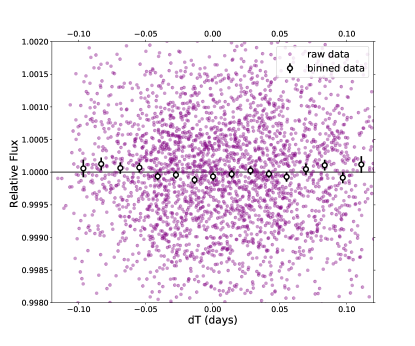
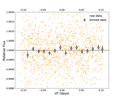
Figure 15: Left: Period-folded photometric measurements obtained by Spitzer IRAC/channel 2 (centered in 4.5 $\mu\mathrm{m}$) near the 28 occultations of planets TRAPPIST-1b, corrected for the measured TTVs. Coloured dots show the unbinned measurements; open circles depict 20min-binned measurements for visual clarity and solid gray line is simply an horizontal line centered in 1.

Right: Similarly but for 9 occultations of TRAPPIST-1c.

To derive the brightness temperature $T_{p,c2}$ from the occultation depths we used the method described in Charbonneau et al. (2005) and Deming et al. (2005). Our starting point was to define the occultation depth as the ratio of the flux of the planet and the total flux outside of transit. This translates into equation (9), where $\Omega_{p}$ is the solid angle subtended by the planet, $\Omega_{\star}$ is the solid angle subtended by the star, $B_{p}$ is the surface brightness of the planet and $B_{\star}$ is the surface brightness of the star,

$$\delta_{occ}=\frac{\Omega_{p}B_{p}}{\Omega_{p}B_{p}+\Omega_{\star}B_{\star}}.$$ (9)

Then, assuming that the planet is a blackbody, its surface brightness $B_{p}$ can be expressed with Planck’s blackbody law,

$$B_{p}(\nu)=\Big{(}\frac{2h\nu^{3}}{c^{2}}\Big{)}\Big{(}\frac{1}{e^{h\nu/k_{b}T_{p}}-1}\Big{)},$$ (10)

where $\nu$ is frequency, $h$ is the Planck constant, $c$ is the speed of light in vacuum, $k_{b}$ is the Boltzmann constant, and $T_{p}$ is the brightness temperature. Equation 10 can be re-arranged as follows:

$$T_{p}(\nu)=\frac{h\nu}{k_{b}\ln\Big(\frac{2h\nu^{3}}{c^{2}B_{p}}+1\Big{missing})}$$ (11)

In addition, when we develop equation (9) we get the ratio $\frac{\Omega_{p}}{\Omega_{\star}}$ which we approximate as the ratio of the planet area with the star area, see equation (12), such that equation (10) becomes equation (13) :

$$\frac{R_{\star}^{2}}{R_{p}^{2}}\simeq\frac{\Omega_{\star}}{\Omega_{p}}$$ (12)

giving

$$B_{p}(\nu)=\frac{\delta_{occ}B_{\star}(\nu)}{1-\delta_{occ}}\Big{(}\frac{R_{\star}}{R_{p}}\Big{)}^{2}.$$ (13)

Finally, substituting equation (13) in equation (11) we obtain the brightness temperature $T_{p}$ as a function of the occultation depth $\delta_{occ}$, the surface brightness of the star $B_{\star}$, and the frequency of the observations, see equation (14) :

$$T_{p}(\nu)=\frac{h\nu}{k_{b}\mathrm{ln}\Big{(}\frac{2h\nu^{3}}{c^{2}\frac{\delta_{occ}B_{\star}(\lambda)}{1-\delta_{occ}}\Big{(}\frac{R_{\star}}{R_{p}}\Big{)}^{2}}+1\Big{)}}$$ (14)

To obtain the value of the star surface brightness $B_{\star}(\nu)$, we followed two different approaches. First, we considered the host star as a blackbody and derive $B_{\star}(\nu)$ from the value of the stellar temperature obtained in Table 4. Secondly, as TRAPPIST-1 is not an ideal blackbody we computed $B_{\star}$ directly from the flux measurements in Spitzer raw images. To do so, we measured the flux of the star in the Spitzer Basic Calibrated Data (BCDs) corrected from instrumental signatures and calibrated in physical units (MJy). We then followed the procedure described in the IRAC Instrument Handbook to obtain the absolute flux density of the star in Spitzer channel 2, such that we multiplied the measured counts by $2.3504*10^{-11}$ $\mathrm{sr}.\mathrm{arcsec}^{-2}$ x $1.22^{2}$ $\mathrm{arcsec}^{2}.\mathrm{pixel}^{-1}$, and then divided by $\Big{(}\frac{R_{\star}}{d}\Big{)}^{2}$ to get the flux density in $\mathrm{W}.\mathrm{m}^{-2}.\mathrm{Hz}^{-1}.\mathrm{sr}^{-1}$, $R_{\star}$ being the radius of TRAPPIST-1 and $d$ the distance of the system from GAIA/DR2. Results from both approaches are presented in Table 9.

Planet	# occultations	$3-\sigma$ upper limit brightness temperature from BB assumption [$K$]	$3-\sigma$ upper limit brightness temperature from measured flux [$K$]
b	28	743	768
c	9	812	842

Table 9: 3$\sigma$ upper limit brightness temperatures computed from the occultation depth outputs by the MCMC analysis carried out in Section .2 (values given in Table 9) using equation(11). The brightness temperature is a function of the surface brightness of the star that was either computed using a blackbody model (BB) or derived from the fluxes measured in the Spitzer telescope raw images of TRAPPIST-1.

Even though we did not significantly detect any occultation signal, we can compared the occultation depths outputs by the MCMC analysis and its 3-$\sigma$ uncertainty with planetary thermal emission models. On Figure 16, we compare the secondary eclipse spectrum models of TRAPPIST-1b and c for different simulated atmospheric models from Lincowski et al. (2018) with the values derived from our analysis. With Figure 16 our intention is not to fit a model to the 3-sigma occultation depth measurement but rather to be informative on the level of signal that needs to be reached to draw conclusions from thermal occultations, and how our Spitzer occultation measurements compare to that. We observe that, for all atmospheric scenarios explored in Lincowski et al. (2018) for TRAPPIST-1b and c, the expected occultation depths are significantly smaller than the 3-$\sigma$ precision that can be reached with existing Spitzer IRAC channel 2 measurements.

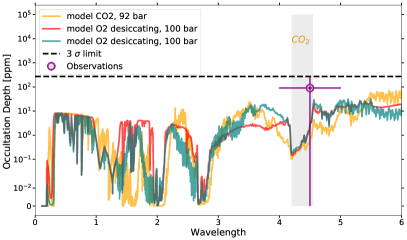
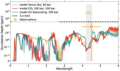
Figure 16: Left: Secondary eclipse spectrum models of TRAPPIST-1b for different assumptions on its atmospheric composition, as simulated by Lincowski et al. (2018), over-plotted with our empirical value, derived from the global analysis of 28 occultations observed with Spitzer IRAC/channel 2 (centered in 4.5 $\mu\mathrm{m}$), the error bar shown corresponds to the 3-$\sigma$ confidence interval of the measurement. The y-axis has a logarithmic scale. The shade gray band stands for the zone where a spectral absorption from $\mathrm{CO}_{2}$ molecule - if present in the atmosphere - is expected. Right: Similar but for TRAPPIST-1c.

From Table 9 the 3-$\sigma$ upper limit brightness temperatures derived from observations are $\sim$ 750 K and $\sim$ 830 K for TRAPPIST-1b and c, respectively. By comparison, the equilibrium temperatures of TRAPPIST-1b and c are $\sim$ 400 and $\sim$340K, respectively, assuming a null albedo. If we make the additional assumptions that the planets are (i) in synchronous rotation – which is one of their most likely spin state (Turbet et al., 2018; Makarov et al., 2018) – and (ii) that they are devoid of atmosphere, then we calculate that equilibrium temperatures on the dayside of TRAPPIST-1b and c are $\sim$ 510 and $\sim$430K, respectively. In a thick atmosphere, the energy coming from the absorption of stellar radiation by the planet on a $\pi$R${}_{\text{p}}^{2}$ area is efficiently redistributed over the surface of the planet of 4$\pi$R${}_{\text{p}}^{2}$ area, leading to a dilution factor of 4. On an airless, synchronously rotating planet, the dilution factor is 1.5 due to the absence of heat redistribution combined with geometric factors. Koll (2019) provides an analytic framework to estimate this factor.

As a result, our $3-\sigma$ confidence measurements of occultation depths for both planets are not sufficient to rule out the presence or absence of an atmosphere, and cannot be used to infer the spin states of the planets. They can be used in principle to set an upper limit on the tidal heat flux of the planet, but tidal calculations have shown it should be on the order of 0.1-40 W m^-2 (Turbet et al., 2018; Barr et al., 2018; Papaloizou et al., 2018; Dobos et al., 2019), depending on the tidal dissipation factor assumed and eccentricity assumed and/or calculated. These tidal heat fluxes are more than two orders of magnitude lower than the irradiation received on TRAPPIST-1b and should thus not contribute in any way to the thermal infrared flux emitted by the planet.

From the results presented in Table 9, we can also speculate what kinds of atmosphere would theoretically induce brightness temperatures higher than our measured upper limit in order to eliminate those scenarios for planet b and c. To maximize thermal emission between 4 and 5 $\mu\mathrm{m}$ (i.e., in the Spitzer IRAC channel 2), we can build a virtual planet with a thick atmosphere that absorbs strongly at all wavelengths (specifically at wavelengths superior to 5 $\mu\mathrm{m}$), except in the 4-5 $\mu\mathrm{m}$ spectral range. To be in agreement with our upper estimate measurements of occultation depths (see Table 9), we calculate (assuming a dilution factor of 4, because here the planet needs to have a thick atmosphere producing a strong greenhouse effect and which is likely to redistribute heat efficiently) that $\sim$ 76$\%$ and $\sim$ 114$\%$ of the total flux absorbed (assuming a null albedo) by TRAPPIST-1b and c, respectively, need to be thermally emitted in the 4-5 $\mu\mathrm{m}$ spectral range. It is very likely impossible for planet b (and virtually impossible for planet c) to build an atmosphere which would emit nearly 100$\%$ of its thermal flux in the 4-5 $\mu\mathrm{m}$ spectral range. This justifies a posteriori why we did not detect any occultation signal of planet b nor planet c.

The most likely yet plausible atmosphere to maximize thermal flux in the 4-5 $\mu\mathrm{m}$ spectral range is a thick $\mathrm{H}_{2}\mathrm{O}$ dominated atmosphere, due to a gap between two infrared absorption bands of $\mathrm{H}_{2}\mathrm{O}$ near 4 $\mu\mathrm{m}$ (Miller-Ricci et al., 2009; Hamano et al., 2015; Katyal et al., 2019). This is one of the most likely scenarios for the atmospheres of the innermost planets of the TRAPPIST-1 system if the planets formed water-rich (rich enough that they survived atmospheric erosion) as supported by some planet formation scenarios (Coleman et al., 2019; Schoonenberg et al., 2019; Izidoro et al., 2019; Bitsch et al., 2019; Raymond et al., 2018) and density measurements (Grimm et al., 2018). This stems from the fact that TRAPPIST-1b and c have incident fluxes beyond the runaway greenhouse limit for which water has been shown to be unstable in condensed form and should rather form a thick H2O-dominated atmosphere (Turbet et al., 2019). Using the thermal emission spectra of Hamano et al. 2015 (e.g., their Figures 1a and 3), we calculate that 15-30$\%$ of the thermal flux is emitted in the 4-5 $\mu\mathrm{m}$ spectral range, depending on the assumption made on the total water content of the planet. For TRAPPIST-1b, this corresponds to a brightness temperature of 470-530 K. These brightness temperatures are similar in magnitude to those calculated for a synchronously rotating, airless planet (equilibrium temperature on the dayside of TRAPPIST-1b of $\sim$ 510 K). This demonstrates how decisive JWST occultation observations of the two TRAPPIST-1 inner planets must be to be able to constrain different realistic scenarios about the nature of these planets.

Additional gases are also likely to quantitatively change these numbers (Marcq et al., 2017; Katyal et al., 2019). Specifically, there is a very strong $\mathrm{CO}_{2}$ absorption band around 4.3 $\mu\mathrm{m}$ which implies that even a small amount of $\mathrm{CO}_{2}$ in the atmospheres of both planets (if any) could mitigate their 4-5 $\mu\mathrm{m}$ brightness, which would limit the ability of the Spitzer/IRAC channel 2 to detect any signal. Again, the large spectral coverage of the various instruments of JWST (NIRSpec, MIRI) combined with their expected high sensitivity will be of great use to constrain these types of atmospheres.

3.3 Flares

The study of flares is essential to obtain insights into planetary evolution and the potential presence of life on extrasolar planets. On one hand, intense flare activity can induce strong atmospheric erosion and make the surface of a planet uninhabitable (Lammer et al., 2007), but on the other hand flares could be a key element to the emergence of life (Airapetian et al., 2016; Ranjan et al., 2017). Indeed, a minimum flaring activity seems beneficial to the formation of the ribonucleotides that will allow ribonucleic acid (RNA) synthesis and initiate prebiotic chemistry afterwards, as presented by Rimmer et al. (2018). This latter work outlines that further analyses of the frequencies of energetic flares around stars later than M4 are necessary to assess the habitability of temperate planets around the lowest-mass stars. Rimmer et al. (2018) also recommend concentrating on very energetic flares because of higher risks of uncertainties and contradictory findings with low energy flares. In this context, we looked for high energy flares in our extensive Spitzer data set and isolated the 5 largest-amplitude flares, 3 of them being caught during the continuous period of observations in 2016. This includes flares previously discussed by Davenport (2017) (flare #1, #2, #3) and two new flares (flare # 4 and # 5). We analyzed the corresponding light curves with the same MCMC code used to analyze the transits and occultations (see Section 2), as it also includes a flare model represented by a instantaneous flux increase followed by an exponential flux decrease. This flare model is embodied by equation 15:

$$F_{\mathrm{flare},t}=\mathrm{Amplitude}_{\mathrm{flare}}\times e^{\Big{(}\frac{-dt}{\tau_{\mathrm{flare}}}\Big{)}}$$ (15)

where $dt=t-t_{0}$ ($t_{0}$ being the time of the instantaneous flux increase), $\tau_{\mathrm{flare}}$ is the flux decrease timescale, and $\mathrm{Amplitude}_{\mathrm{flare}}$ is the flux increase amplitude.

The parameters resulting from our fits are presented in Table 10 and the corresponding light curves are displayed in Figure 17. We estimated the quality of the fit through the Gelman & Rubin test, and for all light curves the Gelman & Rubin coefficient was below $1.1$.

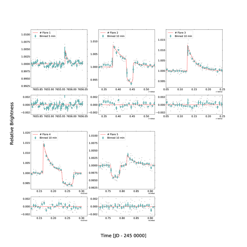
Figure 17: Light curves of the five highest amplitude flares found in our Spitzer time-series photometry. Some flares happened soon after/before a transit. The light curves are ranked in chronological order and a number is associated with each flare.

Table 10 gives the flare parameters obtained from those fits. From those values we computed estimates of the bolometric luminosity of each flare. To do so we followed the procedure described by Shibayama et al. (2013), that is to say we estimated the total energy of each flare from its amplitude and duration combined to the stellar luminosity (see below), by assuming that the spectrum of a flare can be described by a black body function with an effective temperature of $T_{flare}$ $\simeq$ $9000K$. The justification for this assumption came from the observation of Kowalski et al. (2010), and was reinforced in other works like Kretzschmar (2011).

Assuming that the star is a blackbody radiator, the bolometric flare luminosity can be defined as equation:

$$L_{\mathrm{flare,bol}}=\sigma_{SB}T_{\mathrm{flare}}^{4}A_{\mathrm{flare}},$$ (16)

where $\sigma_{SB}$ is the Stefan-Boltzmann constant, $T_{\mathrm{flare}}$ is the black-body temperature of the flare, and $A_{\mathrm{flare}}$ is the area of the flare.

Then, to estimate $A_{\mathrm{flare}}$, we used the observed luminosity of the star ($L_{\star}$), the luminosity of the flare ($L_{\mathrm{flare}}$) defined by equation (17), where the integration is made for the 3.72 - 5.22 $\mu\mathrm{m}$ band pass (corresponding to IRAC/channel 2 spectral range in which all flares were observed) :

$$L_{\mathrm{flare,c2}}(t)=A_{\mathrm{flare}}(t)\int R_{\lambda}B_{\lambda}(T_{\mathrm{flare}})d\lambda$$ (17)

and the flare amplitude of the light curve $\frac{\Delta F(t)}{F(t)}$ defined as equation (18) :

$$\frac{\Delta F(t)}{F(t)}=\frac{L_{\mathrm{flare,c2}}(t)}{L_{\star}}.$$ (18)

In equation (17), $R_{\lambda}$ stands for the spectral response function of Spitzer/IRAC instrument and $B_{\lambda}$ is the Planck function. From equations (17) and (18), we can derive $A_{\mathrm{flare}}$, see equation (19) :

$$A_{\mathrm{flare}}=\frac{\Delta F(t)}{F(t)}\pi R_{\star}^{2}\frac{\int R_{\lambda}B_{\lambda}(T_{\mathrm{eff}})d\lambda}{\int R_{\lambda}B_{\lambda}(T_{\mathrm{flare}})d\lambda}$$ (19)

Finally, the total bolometric energy of the flare ($E_{\mathrm{flare}}$) is defined as the integral of $L_{\mathrm{flare,bol}}$ over the flare duration, equation (20) :

$$E_{\mathrm{flare}}=\int L_{\mathrm{flare,bol}}(t)dt$$ (20)

As underlined by Shibayama et al. (2013), since the star is not a blackbody radiator, such bolometric energy estimates may have errors of a few tens of percent, too small to affect our inferences described below. The results derived from those calculations are shown in Table 10.

Flare #	Timing $\pm$ 1-$\sigma$ [JD - 2450000]		Amplitude $\pm$ 1-$\sigma$ [%]		Duration $\pm$ 1-$\sigma$ (days)		Flare energy $\pm$ error (erg)
1	7655.97363	0.0038	0.635	0.39	0.00759	0.0045	8.41 E+31	5.08e+31
2	7659.38103	0.00051	0.846	0.065	0.04508	0.0072	6.64 E+32	4.02e+32
3	7667.12545	0.00052	1.276	0.092	0.0264	0.0034	5.79 E+32	3.50e+32
4	8021.16339	0.00052	0.148	0.093	0.0248	0.0029	6.41 E+31	3.87e+31
5	8046.8164	0.0011	0.346	0.048	0.030	0.016	1.81 E+32	1.09e+32

Table 10: Output from the individual MCMC analyses of the light curves with the 5 highest energy flares. Timing, amplitude, and duration are measured through a MCMC analysis of the corresponding light curves, while the flare energy is computed by applying equation (20) and its error is estimated to be $\pm$ 60% of the flare energy following the recommendations of Shibayama et al. (2013)

The values that we obtained are consistent with flare energies amplitudes given by Paudel et al. (2018) and Vida et al. (2017) (energy range from ($0.65$ - $710$) $\times 10^{30}$ erg). In Figure 18, we compare the flare frequency distribution of TRAPPIST-1 from our measurements to the frequencies reported in those works. This figure is a log-log plot of cumulative frequency of flare energies; for instance, the cumulative frequency of flares with an energy E is the number of flares with energies superior or equal to E per day.

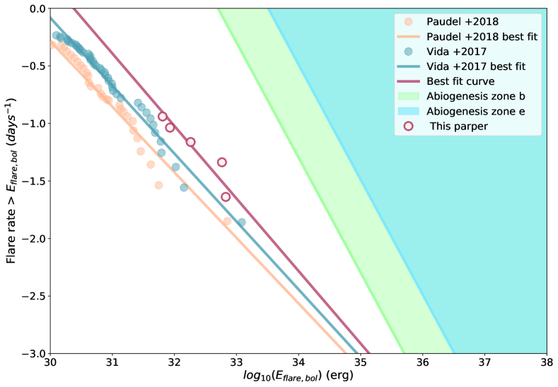
Figure 18: Flare frequency distributions (FFD) in log-log scale, x-axis is the flare energy and y-axis is the cumulative rate of flares per day, that is to say how many flares of a corresponding energy E -or higher- happen per day. Solid lines represent the linear regressions defined by equation (21). The red solid line stands for the result from this work while the orange line stands for results from Paudel et al. (2018) and the green one from Vida et al. (2017). The green zone denotes the abiogenesis zone for planet TRAPPIST-1b, a zone where the inequality (22) is satisfied, the green bold line on the edge of the zone represent the minimum flare rate and energy required to trigger prebiotic chemistry on this planet (Rimmer et al., 2018), which corresponds mathematically to equation (22). The blue zone is similar to the green zone but for planet TRAPPIST-1e.

We noticed that the flare energy distribution of TRAPPIST-1 follows a power law as equation (21):

$$log(\nu)=\beta log(E)+\alpha,$$ (21)

where $\nu$ is the frequency, and $\beta=-0.6303\pm 0.1358$, fitted from our measurements. This value is consistent with the $\beta=-0.61\pm 0.02$ derived by Paudel et al. (2018).

As TRAPPIST-1 is an ultracool dwarf star and its habitable zone planets are particularly close to their host, the question of whether those planets could harbour life in such radiation environments naturally arises (O’Malley-James & Kaltenegger, 2017; Glazier et al., 2019). Within this context, we discuss the meaning of our results in terms of habitability; notably on how flares can promote the emergence of life. To do so, we based our discussion on the work of Rimmer et al. (2018), where the authors explain how the synthesis of pyrimidine ribonucleotides - part of the building blocks of RNA - from hydrogen cyanide and bisulfite in liquid water is likely driven by photochemical processes in the presence of ultraviolet (UV) light. From experiments, the authors defined the “abiogenesis zones” around stars of different stellar types depending on whether their UV fluxes provide sufficient energy to build a sufficiently large prebiotic inventory (Rimmer et al., 2018). Using the flare estimates of Rimmer et al. (2018), modified to account for the semi-major axes of the TRAPPIST-1 planets (Günther et al., 2020, their Eq. (10)), we derived the flare frequencies, $\nu$, for which UV flux received by each TRAPPIST-1 planets would be sufficient for the planet to lie in the abiogenesis zone. Those frequencies are defined by the equation:

$$\nu>25.5\mathrm{day}^{-1}\Big{(}\frac{10^{34}\mathrm{erg}}{E_{\mathrm{U}}}\Big{)}\Big{(}\frac{a}{1\mathrm{AU}}\Big{)}^{2}$$ (22)

where $\nu$ is a function of the flare’s U-band energy $E_{\mathrm{U}}$, the stellar radius, $R_{\star}$, and the stellar temperature, $T_{\star}$. To solve inequation (22), we need the U-band energy $E_{\mathrm{U}}$ and the semi-major axis $a$. We took the semi-major axis from the refined parameters value (see Table 4 in Section 3.1) and we obtained the U-band energy from the bolometric energy through the integration of the flux density in the U-band spectral response function, like it was done by Günther et al. (2020) (see equation 23). We assumed that the flux density of the flare could be expressed as a 9000 K blackbody. We estimate that 6.6788% of the flare’s bolometric energy belongs to the U-band, $E_{\mathrm{U}}\simeq 6.7\%E_{\mathrm{flare}}$.

$$E_{\mathrm{flare},\mathrm{U-band}}=\int_{t}A_{\mathrm{flare}}\int_{Uband}R_{\lambda}B_{\lambda}(T_{\mathrm{flare}})d\lambda dt$$ (23)

We over-plot the abiogenesis zone in terms of flare frequency and energy on Figure 18 for planet TRAPPIST-1e; in other words, a zone where the inequality 22 is satisfied. We chose planets b and e because e is the planet that is the most likely to harbor liquid water on its surface (Wolf, 2017, 2018; Turbet et al., 2018; Fauchez et al., 2019) and b is the closest to the host star. We note that a planet could lie in the abiogenesis zone while not being in the classical habitable zone (Rimmer et al., 2018), yet, by choosing to study planet e we maximize the similarities with Earth.

In Figure 18, if TRAPPIST-1’s power-law flare rates would have crossed the power law of inequality 22 - represented by the blue zone on the Figure - it would have potentially meant that TRAPPIST-1e was located within the abiogenesis zone of its host star. However, we see that TRAPPIST-1’s power-law flare rates do not cross the blue zone. This means that TRAPPIST-1e currently does not receive enough UV flux to build up the prebiotic inventory photochemically. We note that the same interpretation can be made for planet b (the abiogenesis zone of b being the green patch on Figure 18).

Nevertheless, TRAPPIST-1 is an old M8V type star ($7.6\pm 2.2$ Myr old according to Burgasser & Mamajek 2017) and empirical observations showed a decrease of the activity of ultracool dwarfs with age. Indeed, Paudel et al. (2019) compared the flare frequency distribution of 2M0837+2050 - a young $\simeq$ 700 Myr old M8 type star - with TRAPPIST-1 - an old 7.6 Gyr old M8 type star - and found that the highest flare energy on 2M0837+2050 are $\simeq$3 times larger than the ones on TRAPPIST-1, and that a flare of energy E=$10^{34}$erg has 10 times more chances to happen on 2M0837+2050 than on TRAPPIST-1. Considering that those two stars have a similar spectral type (M8 type) but different ages this argument could be used to hypothesize that TRAPPIST-1 used to show more energetic and more frequent flares in its youth. Both Ranjan et al. (2017) and Rimmer et al. (2018) discuss this scenario and argue that flares may be the only means to generate the building blocks of life via the pathways of Xu et al. (2018) and Patel et al. (2015). Furthermore, contrary to the classical habitable zone, it is not required that a planet remains in the abiogenesis zone of its star to maintain the presence of life. This would imply that planet e might have received enough UV flux in its history to drive the emergence of life’s building blocks.

Unfortunately, those interpretations are drawn from empirical studies and are limited by the number of flaring M8 type stars studied so far. Specifically, it remains to be seen whether there is a “golden mean” for flare rates, at which there are enough SEP’s to form feedstock molecules needed for prebiotic chemistry, and enough NUV light to drive that prebiotic chemistry, but not so much XUV light and SEP’s that the atmosphere is stripped (Garraffo et al., 2017; Dong et al., 2018), continually transformed (Vida et al., 2017; Tilley et al., 2019), or the planet desiccated (Luger & Barnes, 2015). This ’golden mean’ for flare rates only applies for host planets outside the abiogenesis zone as delineated by quiescent stellar NUV flux. For those planets outside the abiogenesis zone, stellar activity would be the only means to generate sufficient NUV for this prebiotic chemistry. The Earth has resided well within the abiogenesis zone throughout its history.

It should be emphasized that the abiogenesis zones delineated by Rimmer et al. (2018); Günther et al. (2020) and in this work are scenario-dependent. It may be that life’s building blocks can arise another way, either within hydrothermal vents (Rimmer & Shorttle, 2019), in surface scenarios without ultraviolet light (Rimmer & Shorttle, 2019), or that they may be delivered exogenously (Rimmer & Shorttle, 2019). In addition, within the scenario explored by Rimmer et al. (2018), the threshold UV flux provides a necessary but not sufficient condition for the origins of life on a rocky planet. Hydrogen cyanide, bisulfite and phosphate must be present at high concentrations within liquid water, along with other chemical constituents (Patel et al., 2015; Xu et al., 2018). Given these added conditions, it is likely that each major category of life’s building blocks: amino acids, phospholipids, nucleotides, would be present in high concentrations, along with a mechanism for joining them together to form macromolecules: proteins, phospholipid membranes, RNA and DNA (Liu et al., 2019). The problem of how life arises from this system, or any complex molecular system, remains unsolved.

3.4 Search for a additional transiting objects

One of the primary goals of the Red Worlds program was to search for additional transiting planets. In this context, we ran a Transit Least Square analysis (TLS) with period spanning from 0.2 to 200 days on the residuals of the full photometric dataset corrected from all known transits. The TLS algorithm, presented by Hippke & Heller (2019), aims to detect transit-like features from time-series photometry while taking the stellar limb-darkening, the planetary ingress and egress into account. The TLS algorithm is particularly relevant here as it is optimized for small planets and was found more reliable than the Box least Square (BLS) algorithm in finding any kind of planets by Hippke & Heller (2019). We combined this with a visual inspection of all the light curves. Results are shown on Figure 19, this figure was obtained using the Transit Least Squared (TLS) python package by Hippke & Heller (2019).

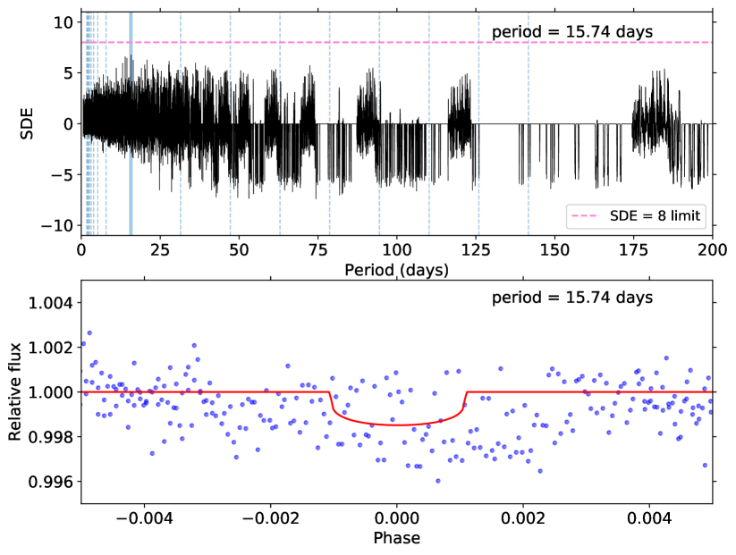
Figure 19: Top panel: Periodogram computed with the help of the Transit Least Squared (TLS) python package (Hippke & Heller, 2019) applied to the time series made by the residuals of the entire Spitzer photometric (cleaned from all known transits). The x-axis is the period while the y-axis is the Signal Detection Efficiency (SDE) associated with each period. A steel-blue line indicates the harmonic for which the SED reached is the largest, here this output period is 15.74 days. Bottom panel: Phase-folded transit signal for the most probable period output by the periodogram (blue dots) + transit model computed from the parameters output by the TLS algorithm (red solid line).

The periodogram peaks at 15.7397 days period, yet this result must be interpreted with care as the maximum value of the SDE for this period is only 6.767 whereas Pope et al. (2016) recommend to consider planetary candidate only for Signal Detection Efficiency (SDE) ¿ 8. The SDE being define as $SDE=max(power/std_{power})$. Besides, the depth of the corresponding phase folded transit signal is relatively small (1487 ppm) and of the same order of magnitude as the dispersion of out-of-transit measurements (standard deviation $\simeq$ 1987 ppm) (Figure 19 bottom panel). In a nutshell, those results favors a non physical explanation (most probably systematics) for this periodic signal spotted at 15.7397 days by the TLS algorithm. We did not consider any other periods in the periodogram as their SDE were always inferior to 8 Pope et al. (2016).

Howerver, one thing we can do is to compute the photometric precision that can be reach as a function of period, then inject planets with signal-to-noise ratio (S/N) of 8 at each period and see if we recover them with TLS. Such results can help us define which kind of hypothetical ninth planet can be discarded from Spitzer’s photometry. Figure 20 shows the precision that we get from the photometry for a set of periods going from 0.2 to 200 days. To construct this figure we have folded the data on each period, for a set of transit timings such that the full period is covered, binned them and computed the standard deviation of this binned light curve, this standard deviation is what we refer to as the photometric precision reached on a given period. The minimum planet radius (hereafter $R_{p,min}$) was then derived from a depth equivalent to a S/N of 8. Where the S/N is expressed as $S/N=\frac{dF}{\sigma}*\sqrt{N}$, with $\sigma$ the precision at a given period and N the number of points in transit, as defined by Pont et al. (2006).

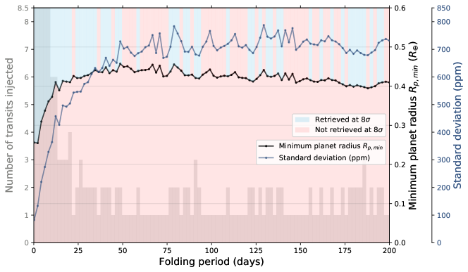
Figure 20: Evolution of the photometric precision and its corresponding planet radius for S/N = 8 as a function of the folding period. The number of injected transits for each period is given by the plot bar in gray. The blue patches show the periods for which the ”injected planet” is recovered where as the red patches show the periods for which it is not.

Assuming an hypothetical planets with circular orbit and null impact parameter, we observe that our precision on the dataset is good enough to detect any Mars-sized planet with period inferior to $\simeq$ 45 days (with an S/N of 8), and good enough to detect any Earth sized planet that would have a period between 0.2 and 200 days (with an S/N of 8). We observe that above P $\simeq$ 50 days the precision seems to stagnate, this is due to the fact that gaps exist in the dataset such that at some point only one event is used to construct the period-folded light curve for most of the periods. Yet, as the duration of the transit increases with the period and the precision stays more a less constant for P $\geq$ 50, the minimum planetary radius that we can detect with S/N=8 tends to decrease for P $\geq$ 50. To second those results we performed some transits injection/retrieval, the retrieval phase being essentially the capacity to find back the injected transits with an SDE ¿ 8 when performing a TLS analysis on the residual + injected transits. The retrieval is obviously greatly dependent on the transit timing used as reference, as a scenario where no transits fall in the observations is likely. Therefore, we imposed this reference timing to be within Spitzer’s time series such that for all periods there is at least one transit in the data. The parameters of the injected transit are chosen as follow: - its period P is the main variable, - its depth $df_{p}$ is such that $S/N=8$, with the S/N as defined above - its width $T_{14,p}$ is calculated analytically from $df_{p}$ and P assuming a circular orbit and a null impact parameter.

As a result, TLS do recover all the injected planets with an SDE ¿ 8 as long as at least 2 transits fall in the data, see figure 20 . Hence, if present we should have detect any Mars-sized planet with period inferior to $\simeq$ 50 days and all Earth sized planet with P ¡ 200 days providing at least 2 of its transits happened during the observations.

To complement this analysis, we conducted a careful visual inspection of the light curves to catch any single occurrence event that could have been missed by the TLS. We found four orphan transit-like structures that did not correspond to any known planetary transit and that we could not model with any function of external parameters (e.g., x- and y-position of the star on the IRAC chip, fwhm variation and ramp effect). Therefore, we treated those events as possible transits of unknown transiting objects and tried to fit them with our MCMC code (see Section 2). We choose to freely vary the period and the impact parameter while assuming priors on the transit depth, the eclipse duration and the transit timing with large error bars that we estimated visually. For the stellar parameters, we used the same priors as for our individual transit analysis (see Section 2.2.1). The results from those analyses can be found in Table 11 and the visualization of the fits is shown on Figure 21.

Orphan #	Timing $\pm$ 1-$\sigma$ [JD - 2450000]		Depth $\pm$ 1-$\sigma$ [%]		Duration $\pm$ 1-$\sigma$ (days)		Impact parameter $\pm$ 1-$\sigma$		Period $\pm$ 1-$\sigma$ (days)
#1	7658.47094	0.00110	0.463	0.091	0.0287	0.0039	0.920	0.058	17	10
#2	7666.28113	0.00058	0.151	0.068	0.048	0.012	0.83	0.36	59	42
#3	7671.45227	0.00053	0.249	0.146	0.0185	0.0017	0.65	0.42	1	2
#4	8045.11500	0.00230	0.198	0.091	0.0331	0.006	0.903	0.062	34	28

Table 11: Outputs from the individual MCMC analysis of four transit-like structures found in Spitzer’s photometric observations of TRAPPIST-1. Convergence of our analyses was assessed with the Gelman & Rubin test (Gelman & Rubin, 1992) (lower that 1.1 for all jump parameters).

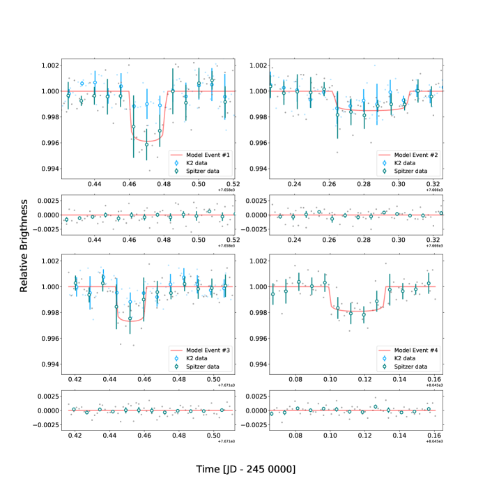
Figure 21: Visualization of the fits of the light curve of the four transit-like structures found in Spitzer photometry. Gray dots show the unbinned measurements for Spitzer; green open circles depict 10 min-binned measurements for visual clarity. The best-fit transit models are shown as red solid lines. Events are ranked and assigned a number corresponding to their chronological order: Top-left is event #1, top-right is event #2, bottom-left is event #3 and bottom-right is event #4. When available K2 simultaneous measurements are over-plotted in blue dots with 10 min-binned measurements as blue open circles.

From Table 11, we note that if those events were associated with one or more transiting objects this object would be highly grazing as the impact parameters output from our fit are all larger than 0.6. Yet, we observe that the differences in duration and amplitude between events # 1, 2, 3 and # 4 tend to discard a common origin scenario. Event # 3 was caught in a particularly noisy AOR so even if the light curve structure can not be removed with any baseline detrending, we are doubtful this is a physical transit. As a general comment, event # 1, 2 and 3 were caught during the second campaigns which, as mentioned before, had some known drifting issues due to the use of inaccurate pointing coordinates, weakening our confidence in the detrending performed. Besides, none of the timings of those orphan transits are included in the transits timings associated to the TLS most favored period of 15.74 days. Furthermore, at the time of event # 1, 2 and 3 we found out that some K2 observations were carried out simultaneously but the data do not confirm any of the structures we identifies, which strongly weaken any astrophysical origin scenario. Finally, event # 4 is rather shallow $\simeq$ 0.2 % and of similar order than the out-of-transit dispersion ($\simeq$ 0.12%), the event being significant at the $1.6\sigma$ level only.

In a nut shell, the 4 orphans structures identified seem to be emerging from a nonperfect correction of systematics effects rather than an eighth transiting object.

4 Conclusion

The Spitzer Exploration Program Red Worlds is among the largest programs undertaken with the Spitzer Space Telescope and has gathered more than 1000 hours of observation of the touchstone TRAPPIST-1 system. First, we emphasize that this program has largely met its expectations, notably through the discovery of 4 new planets orbiting the TRAPPIST-1 star, all well-suited for detailed atmospheric characterization with next-generation telescopes (Gillon et al., 2017), as well as for the assessment of the variability of the host star (Delrez et al., 2018), and the determination of planet masses and orbital parameters through the transit timing variations method (Grimm et al., 2018). In this work, we presented the analysis of all the transits of the TRAPPIST-1 planets observed with Spitzer/IRAC from February 2016 to March 2018 within the framework of the Red Worlds program. Our approach to analyze this exquisite data-set and our most relevant results are summarized as followed:
- We refined both the stellar and transit parameters through global analyses of the entire dataset, which enabled us to revise the planets’ physical parameters (see table 4).
- We also performed a global analysis for each planet, and individual analyses of each transit, to search for signs of stellar contamination either of spectral or photometric nature. We did not find clear evidence of stellar contamination in the transit light curves, in agreement with Morris et al. (2018c).
- Comparing our individual and global analyses of the transits, we estimate for TRAPPIST-1 transit depth measurements mean noise floors of $\sim$35 and 25 ppm in channels 1 and 2 of Spitzer/IRAC, respectively. We estimate that most of this noise floor is of instrumental origins and due to the large inter-pixel inhomogeneity of IRAC InSb arrays, and that the much better inter-pixel homogeneity of JWST instruments should result in noise floors as low as 10ppm, low enough to enable the atmospheric characterization of the planets by transit transmission spectroscopy. - On the spectral side, similarly to Ducrot et al. (2018) and Burdanov et al. (2019), we concluded that the transmission spectra of the TRAPPIST-1 planets are not flat and that Zhang et al. (2018)’s fit derived from the stellar contamination model from Rackham et al. (2018) agrees relatively well with the 7 planets’ combined observations, apart from the Spitzer observational point at $3.6\mu\mathrm{m}$. Nevertheless, because of existing discrepancies in the near-IR between measurements from different instruments it is still too early to confirm that those spectral features originate from stellar contamination.
- Then, we searched for an occultation signal but did not detect any, even with 28 occultations of b and 9 occultations of c. Yet, we were able to set an upper constraint on the dayside brightness temperature of b and c. Those upper limits on the temperatures were so high that it appears impossible for planet b and c to build virtual atmospheres that would be in agreement with our upper estimate measurements of occultation depths. This justifies a posteriori why we did not detect any occultation signal of either planet b or planet c.
- We then compared realistic atmospheric models with our derived transmission/emission spectra and emphasized that even with a large number of transits observed with Spitzer/IRAC, interpretations are still limited by the current precision on the measurements. Only the combined transit transmission spectrum of several planets (b+c+d+e+f+g) lowered our error bars enough to open discussions on the presence/absence of certain molecular absorbers. This combined spectrum suggests that it is unlikely that most of the TRAPPIST-1 planets possess $\mathrm{CH}_{4}$-dominated atmospheres, yet this interpretation was made from only two observational points (Spitzer IRAC channels 1 and 2) and therefore requires further investigation. This observation highlights the even more crucial role of the future James Webb Space Telescope to shed light on the presence or absence of atmospheres around the TRAPPIST-1 planets, and their subsequent characterization.
- We also computed the flare frequency distribution of the planets and observed that none of them currently lies in the abiogenenis zone of their host, meaning that the actual flaring activity is currently too weak to initiate prebiotic chemistry via the mechanism detailed in Xu et al. (2018); Rimmer et al. (2018). However, TRAPPIST-1 is believed to be old and flaring activity is believed to decrease with star’s age meaning that the planets could have received the appropriate amount of UV energy in their past.
- Last but not least, we identified four orphan transit structures in the dataset that we could not link to any known planet. However, three of those structures are not confirmed by simultaneous K2 data and the last one is not significant at more that the 2$\sigma$ level. These structure could be the result of unknown external systematical effect.

The most recent observations of the TRAPPIST-1 system with Spitzer were performed in October 2019, and will unfortunately be the last. But on a brighter note, the James Webb Space Telescope is on its way to take over and yield even more insight into this extraordinary system.

Appendix A Description of the data

Table 12: Baseline for the individual analysis of each transit

Date	Number of Points	Epoch	Baseline	$\beta_{w}$	$\beta_{r}$	CF	Channel
TRAPPIST-1b
2016-02-21	108	78	$p(t^{3})$+$p(fwhm_{x}^{1})$+$p(xy^{1})$	1.09	1.0	1.09	c2
2016-03-04	132	86	$p(xy^{1})$	0.84	1.12	1.06	c2
2016-03-15	164	93	$p(t^{3})$+$p(xy^{1})$	1.01	1.07	1.08	c2
2016-09-20	114	218	$p(fwhm_{y}^{1})$+$p(xy^{1})$	1.05	1.08	1.13	c2
2016-09-21	665	219	$p(xy^{1})$	1.04	1.21	1.25	c2
2016-09-26	132	222	$p(fwhm_{y}^{1})$+$p(xy^{1})$+$p(r^{1})$	1.03	1.31	1.35	c2
2016-09-29	135	224	$p(t^{1})$+$p(xy^{1})$	0.97	1.04	1	c2
2016-09-30	56	225	$p(t^{1})$+$p(xy^{1})$	0.75	1.21	0.9	c2
2016-10-05	141	228	$p(xy^{1})$	0.87	1.04	0.91	c2
2016-10-07	126	229	$p(xy^{1})$	0.99	1.13	1.12	c2
2016-10-08	127	230	$p(t^{2})$+$p(xy^{1})$	0.96	1.09	1.05	c2
2017-02-18	67	318	$p(xy^{1})$	0.99	1.0	0.99	c2
2017-02-21	70	320	$p(xy^{1})$	0.91	1.0	0.91	c2
2017-02-23	67	321	$p(t^{1})$+$p(fwhm_{y}^{1})$+$p(xy^{1})$+$p(r^{1})$	0.97	1.0	0.97	c2
2017-02-24	67	322	$p(t^{1})$+$p(fwhm_{y}^{1})$+$p(xy^{1})$	0.86	1.15	0.93	c1
2017-02-27	105	324	$p(xy^{1})$+$p(r^{1})$	0.92	1.0	0.92	c2
2017-03-01	74	325	$p(fwhm_{x}^{1})$+$p(xy^{1})$	0.81	1.09	0.9	c2
2017-03-02	67	326	$p(fwhm_{y}^{1})$+$p(xy^{1})$	0.72	1.28	0.92	c1
2017-03-04	67	327	$p(fwhm_{y}^{1})$+$p(xy^{1})$+$p(r^{1})$	0.93	1.0	0.93	c1
2017-03-05	74	328	$p(xy^{1})$	1.03	1.0	1.03	c2
2017-03-07	67	329	$p(fwhm_{y}^{1})$+$p(xy^{1})$	0.87	1.18	1.03	c1
2017-03-08	67	330	$p(t^{1})$+$p(fwhm_{y}^{1})$+$p(xy^{1})$	0.87	1.14	0.97	c1
2017-03-11	68	332	$p(xy^{1})$	1.13	1.0	1.13	c2
2017-03-13	67	333	$p(t^{2})$+$p(fwhm_{x}^{1})$+$p(fwhm_{y}^{1})$+$p(xy^{1})$	0.84	1.15	0.96	c1
2017-03-14	67	334	$p(fwhm_{y}^{1})$+$p(xy^{1})$	0.79	1.39	1.11	c1
2017-03-16	67	335	$p(t^{1})$+$p(fwhm_{y}^{1})$+$p(xy^{1})$	0.87	1.51	1.31	c1
2017-03-20	67	338	$p(t^{1})$+$p(fwhm_{y}^{1})$+$p(xy^{1})$	0.66	1.07	0.71	c1
2017-03-22	67	339	$p(t^{1})$+$p(fwhm_{y}^{1})$+$p(xy^{1})$	0.76	1.0	0.76	c1
2017-03-25	67	341	$p(t^{2})$+$p(fwhm_{x}^{2})$+$p(fwhm_{y}^{1})$+$p(xy^{1})$	0.96	1.0	0.96	c1
2017-03-26	67	342	$p(t^{2})$+$p(fwhm_{y}^{1})$+$p(xy^{2})$	0.61	1.0	0.61	c1
2017-09-13	67	455	$p(t^{1})$+$p(fwhm_{y}^{1})$+$p(xy^{1})$+$p(r^{1})$	0.84	1.21	1.01	c1
2017-09-14	118	456	$p(t^{1})$+$p(xy^{1})$	1.14	1.24	1.42	c1
2017-09-16	67	457	$p(t^{1})$+$p(fwhm_{y}^{1})$+$p(xy^{1})$	0.86	1.0	0.86	c1
2017-09-17	95	458	$p(t^{4})$+$p(fwhm_{y}^{3})$+$p(xy^{1})$+$p(r^{1})$	1.1	1.0	1.1	c1
2017-09-19	67	459	$p(t^{1})$+$p(fwhm_{x}^{1})$+$p(xy^{1})$	1.06	1.0	1.06	c1
2017-09-21	67	460	$p(t^{1})$+$p(fwhm_{y}^{1})$+$p(xy^{1})$	1.17	1.15	1.34	c1
2017-09-24	67	462	$p(fwhm_{x}^{1})$+$p(fwhm_{y}^{1})$+$p(xy^{1})$+$p(r^{1})$	0.9	1.17	1.05	c1
2017-09-28	67	465	$p(t^{2})$+$p(xy^{1})$	0.93	1.0	0.93	c1
2017-10-01	67	467	$p(t^{1})$+$p(fwhm_{y}^{1})$+$p(xy^{1})$	0.84	1.33	1.12	c1
2017-10-03	67	468	$p(fwhm_{x}^{1})$+$p(fwhm_{y}^{1})$+$p(xy^{1})$	0.85	1.21	1.03	c1
2017-10-09	67	472	$p(xy^{1})$	0.88	1.59	1.4	c1
2017-10-10	67	473	$p(fwhm_{y}^{1})$+$p(xy^{1})$	1.01	1.42	1.44	c1
2017-10-13	67	475	$p(t^{1})$+$p(fwhm_{y}^{1})$+$p(xy^{1})$	0.66	1.05	0.69	c1
2017-10-15	67	476	$p(xy^{1})$+$p(r^{1})$	0.87	1.0	0.87	c1
2017-10-16	52	477	$p(t^{2})$+$p(xy^{1})$+$p(r^{1})$	0.9	1.0	0.9	c1
2017-10-18	70	478	$p(t^{2})$+$p(fwhm_{x}^{1})$+$p(fwhm_{y}^{1})$+$p(xy^{1})$	1.13	1.0	1.13	c1
2017-10-19	66	479	$p(t^{1})$+$p(fwhm_{x}^{1})$+$p(fwhm_{y}^{1})$+$p(xy^{1})$	0.84	1.0	0.84	c1
2018-03-09	129	572	$p(fwhm_{y}^{2})$+$p(xy^{1})$	0.97	1.17	1.14	c2
2018-03-10	96	573	$p(fwhm_{x}^{1})$+$p(xy^{1})$	0.99	1.0	0.99	c2
2018-03-19	80	579	$p(xy^{1})$	0.94	1.22	1.16	c2
2018-03-25	68	583	$p(t^{2})$+$p(xy^{1})$	1.1	1.0	1.1	c2
2019-10-01	182	950	$p(t^{1})$+$p(fwhm_{x}^{1})$+$p(fwhm_{y}^{1})$+$p(xy^{1})$	1.06	1.0	1.06	c2
2019-10-10	150	956	$p(t^{2})$+$p(fwhm_{x}^{1})$+$p(fwhm_{y}^{1})$+$p(xy^{1})$+$p(r^{1})$	0.97	1.0	0.97	c2
2019-10-13	180	958	$p(fwhm_{x}^{1})$+$p(fwhm_{y}^{1})$+$p(xy^{1})$	1.05	1.0	1.05	c2
TRAPPIST-1c
2016-03-04	66.0	70	$p(xy^{1})$	1.01	1.0	1.01	c2
2016-09-19	118.0	152	$p(xy^{1})$+$p(r^{1})$	0.88	1.38	1.21	c2
2016-09-21	82.0	153	$p(xy^{1})$+$p(r^{1})$	0.83	1.0	0.83	c2
2016-09-24	108.0	154	$p(xy^{1})$	1.12	1.58	1.77	c2
2016-09-26	111.0	155	$p(xy^{1})$	1.0	1.21	1.22	c2
2016-10-01	134.0	157	$p(fwhm_{x}^{2})$+$p(fwhm_{y}^{1})$+$p(xy^{1})$+$p(r^{1})$	0.86	1.44	1.24	c2
2016-10-06	156.0	159	$p(xy^{1})$	0.98	1.06	1.04	c2
2016-10-08	153.0	160	$p(xy^{1})$	0.82	1.25	1.02	c2
2017-02-18	67.0	215	$p(xy^{1})$	1.03	1.0	1.03	c2
2017-02-21	77.0	216	$p(t^{2})$+$p(xy^{1})$	0.84	1.0	0.84	c2
2017-02-23	67.0	217	$p(xy^{1})$	1.05	1.26	1.32	c2
2017-02-26	67.0	218	$p(fwhm_{x}^{1})$+$p(xy^{1})$+$p(r^{1})$	1.0	1.0	1.0	c2
2017-02-28	67.0	219	$p(fwhm_{x}^{1})$+$p(xy^{1})$	0.93	1.0	0.93	c2
2017-03-03	67.0	220	$p(t^{1})$+$p(fwhm_{x}^{1})$+$p(xy^{1})$	0.95	1.0	0.95	c2
2017-03-05	52.0	221	$p(xy^{1})$	0.95	1.02	0.97	c2
2017-03-07	59.0	222	$p(xy^{1})$	0.9	1.0	0.9	c2
2017-03-10	67.0	223	$p(fwhm_{x}^{1})$+$p(xy^{1})$+$p(r^{1})$	0.9	1.11	0.99	c2
2017-03-12	95.0	224	$p(fwhm_{x}^{1})$+$p(xy^{1})$+$p(r^{1})$	0.99	1.02	1.01	c2
2017-03-15	95.0	225	$p(xy^{1})$+$p(r^{1})$	0.92	1.0	0.92	c2
2017-03-20	67.0	227	$p(t^{1})$+$p(fwhm_{x}^{1})$+$p(xy^{1})$	0.94	1.0	0.94	c2
2017-03-22	67.0	228	$p(fwhm_{y}^{1})$+$p(xy^{1})$	1.01	1.11	1.12	c2
2017-03-24	110.0	229	$p(t^{2})$+$p(xy^{1})$	0.99	1.0	0.99	c2
2017-03-27	67.0	230	$p(fwhm_{x}^{1})$+$p(fwhm_{y}^{1})$+$p(xy^{1})$	0.95	1.47	1.4	c2
2017-09-15	94.0	301	$p(fwhm_{x}^{1})$+$p(xy^{1})$+$p(r^{1})$	1.04	1.54	1.6	c2
2017-09-17	113.0	302	$p(t^{2})$+$p(xy^{1})$	0.95	1.41	1.34	c1
2017-09-24	105.0	305	$p(xy^{1})$	1.04	1.0	1.04	c2
2017-09-27	67.0	306	$p(fwhm_{y}^{1})$+$p(xy^{1})$	0.91	1.21	1.11	c1
2017-10-07	108.0	310	$p(t^{2})$+$p(xy^{1})$	1.07	1.0	1.07	c2
2017-10-11	100.0	312	$p(fwhm_{y}^{1})$+$p(xy^{1})$+$p(r^{1})$	0.82	1.56	1.38	c1
2017-10-14	74.0	313	$p(t^{3})$+$p(xy^{1})$+$p(r^{1})$	0.91	1.46	1.33	c2
2017-10-16	59.0	314	$p(fwhm_{x}^{1})$+$p(fwhm_{y}^{1})$+$p(r^{1})$	1.09	1.02	1.11	c1
2017-10-19	60	315	$p(t^{2})$+$p(fwhm_{y}^{2})$+$p(xy^{1})$+$p(r^{1})$	0.74	1.07	0.8	c1
2018-03-13	65.0	375	$p(t^{1})$+$p(fwhm_{y}^{1})$+$p(xy^{1})$+$p(r^{1})$	0.9	1.03	0.93	c1
2018-03-25	83.0	380	$p(fwhm_{y}^{1})$+$p(xy^{1})$	1.07	1.07	1.15	c2
2018-03-28	98.0	381	$p(t^{1})$+$p(fwhm_{y}^{1})$+$p(xy^{1})$	1.11	1.27	1.4	c1
2019-10-01	182	609	$p(fwhm_{x}^{1})$+$p(fwhm_{y}^{1})$+$p(xy^{1})$	1.06	1.0	1.06	c2
2019-10-08	190	612	$p(t^{3})$+$p(fwhm_{x}^{1})$+$p(r^{1})$	0.95	1.44	1.37	c2
2019-10-13	180	614	$p(fwhm_{x}^{1})$+$p(fwhm_{y}^{1})$+$p(xy^{1})$	1.05	1.0	1.05	c2
2019-10-20	188	617	$p(t^{2})$+$p(fwhm_{x}^{1})$+$p(fwhm_{y}^{1})$+$p(xy^{1})$+$p(r^{1})$	0.97	1.0	0.97	c2
TRAPPIST-1d
2016-09-22	134	-4	$p(fwhm_{x}^{1})$+$p(fwhm_{y}^{1})$+$p(xy^{1})$	1.05	1.34	1.4	c2
2016-09-26	114	-3	$p(fwhm_{y}^{1})$+$p(xy^{1})$	1.1	1.1	1.21	c2
2016-09-30	154	-2	$p(xy^{1})$	1.08	1.59	1.71	c2
2016-10-04	145	-1	$p(fwhm_{x}^{2})$+$p(xy^{1})$	0.76	1.36	1.04	c2
2016-10-08	133	0	$p(xy^{1})$	0.86	1.56	1.35	c2
2017-02-19	122	33	$p(xy^{1})$+$p(r^{1})$	0.94	1.06	0.97	c2
2017-02-23	122	34	$p(xy^{1})$+$p(r^{1})$	0.94	1.0	0.94	c2
2017-02-27	134	35	$p(fwhm_{x}^{1})$+$p(fwhm_{y}^{1})$+$p(xy^{1})$+$p(r^{1})$	0.96	1.04	1	c2
2017-03-03	122	36	$p(xy^{1})$	0.89	1.0	0 ,89	c2
2017-03-07	121	37	$p(xy^{1})$	1.01	1.0	1.01	c2
2017-03-11	120	38	$p(xy^{1})$+$p(r^{1})$	1.09	1.0	1.09	c2
2017-03-15	142	39	$p(t^{2})$+$p(fwhm_{y}^{1})$+$p(xy^{1})$	1.01	1.0	1.01	c2
2017-03-19	122	40	$p(fwhm_{x}^{1})$+$p(xy^{1})$	0.99	1.0	0.99	c2
2017-09-17	120	85	$p(t^{3})$+$p(xy^{2})$+$p(r^{1})$	1.03	1.4	1.44	c1
2017-09-25	122	87	$p(t^{1})$+$p(fwhm_{y}^{1})$+$p(xy^{1})$	0.76	1.76	1.33	c1
2017-10-08	122	90	$p(t^{3})$+$p(fwhm_{y}^{2})$+$p(xy^{2})$	0.75	1.32	0.98	c1
2017-10-16	122	92	$p(t^{2})$+$p(xy^{2})$	0.99	1.69	1.67	c1
2017-10-20	129	93	$p(xy^{1})$+$p(r^{1})$	0.98	1.0	0.98	c2
2018-03-06	183	127	$p(fwhm_{x}^{1})$+$p(xy^{1})$+$p(r^{2})$	1.04	1.21	1.25	c2
2018-03-31	106	133	$p(xy^{1})$	1.01	1.33	1.33	c2
TRAPPIST-1e
2016-09-22	97	-1	$p(xy^{1})$+$p(fwhm_{x}^{1})$+$p(fwhm_{y}^{1})$+$p(r^{1})$	1.00	1.12	1.12	c2
2016-09-28	154	0	$p(t^{1})$+$p(xy^{1})$	0.99	1.0	0.99	c2
2017-02-22	106	24	$p(fwhm_{x}^{1})$+$p(xy^{1})$	1.03	1.24	1.28	c2
2017-02-28	99	25	$p(xy^{1})$+$p(r^{1})$	0.85	1.02	0.87	c2
2017-03-06	141	26	$p(fwhm_{x}^{1})$+$p(xy^{1})$	1.06	1.09	1.15	c2
2017-03-12	124	27	$p(t^{3})$	1.05	1.0	1.05	c2
2017-03-18	134	28	$p(t^{1})$+$p(xy^{1})$+$p(r^{1})$	0.88	1.01	0.89	c2
2017-03-24	127	29	$p(xy^{1})$	0.99	1.0	0.99	c2
2017-09-17	88	58	$p(t^{2})$+$p(xy^{1})$	1.01	1.02	1.03	c1
2017-09-23	122	59	$p(fwhm_{x}^{1})$+$p(fwhm_{y}^{1})$+$p(xy^{1})$+$p(r^{1})$	0.9	1.0	0.9	c1
2017-10-12	113	62	$p(xy^{1})$+$p(r^{2})$	0.93	1.07	1.01	c1
2018-03-07	122	86	$p(fwhm_{y}^{1})$+$p(xy^{1})$+$p(r^{2})$	0.99	1.53	1.5	c1
2018-03-13	71	87	$p(fwhm_{y}^{1})$+$p(xy^{1})$	0.89	1.36	1.22	c1
2018-03-19	161	88	$p(fwhm_{x}^{1})$+$p(xy^{1})$	1.01	1.1	1.12	c2
2018-03-25	113	89	$p(xy^{1})$	0.97	1.03	1.0	c2
2019-10-01	122	180	$p(t^{1})$+$p(fwhm_{x}^{1})$+$p(fwhm_{y}^{1})$+$p(xy^{1})$	1.04	1.42	1.48	c2
2019-10-13	122	182	$p(t^{1})$+$p(fwhm_{x}^{2})$+$p(fwhm_{y}^{2})$	1.06	1.09	1.16	c2
TRAPPIST-1f
2016-09-30	170	-1	$p(xy^{1})$	0.93	1.66	1.54	c2
2016-10-09	200	0	$p(fwhm_{x}^{1})$+$p(fwhm_{y}^{1})$+$p(xy^{1})$	0.87	1.66	1.45	c2
2017-02-24	150	15	$p(t^{1})$+$p(fwhm_{x}^{1})$+$p(xy^{1})$	1.04	1.74	1.81	c2
2017-03-06	124	16	$p(fwhm_{x}^{1})$+$p(xy^{1})$+$p(r^{1})$	0.96	1.06	1.02	c2
2017-03-15	173	17	$p(t^{1})$+$p(fwhm_{y}^{1})$+$p(xy^{1})$+$p(r^{1})$	1.04	1.01	1.05	c2
2017-03-24	138	18	$p(fwhm_{x}^{1})$+$p(xy^{1})$+$p(r^{1})$	0.96	1.48	1.42	c2
2017-09-24	106	38	$p(fwhm_{x}^{1})$+$p(xy^{1})$+$p(r^{1})$	0.88	1.03	0.91	c2
2018-03-09	160	56	$p(fwhm_{x}^{1})$+$p(xy^{1})$	1.02	1.03	1.06	c2
2018-03-18	150	57	$p(fwhm_{x}^{1})$+$p(xy^{1})$+$p(r^{2})$	0.85	1.23	1.04	c1
2018-03-27	148	58	$p(t^{2})$+$p(fwhm_{y}^{1})$+$p(xy^{1})$	1.15	1.31	1.5	c1
2019-10-01	182	118	$p(fwhm_{x}^{1})$+$p(fwhm_{y}^{1})$+$p(xy^{1})$	1.06	1.0	1.06	c2
2019-10-10	150	119	$p(t^{2})$+$p(fwhm_{x}^{1})$+$p(fwhm_{y}^{1})$+$p(xy^{1})$+$p(r^{1})$	0.97	1.0	0.97	c2
2019-10-28	150	121	$p(t^{1})$+$p(fwhm_{x}^{1})$+$p(fwhm_{y}^{1})$+$p(r^{1})$	0.88	1.01	0.89	c2
TRAPPIST-1g
2016-10-03	147	30	$p(fwhm_{x}^{1})$+$p(fwhm_{y}^{1})$+$p(xy^{1})$	0.76	1.64	1.24	c2
2017-03-01	86	12	$p(fwhm_{x}^{1})$+$p(fwhm_{y}^{1})$+$p(xy^{1})$	0.93	1.0	0.93	c2
2017-03-13	150	13	$p(t^{2})$+$p(fwhm_{y}^{1})$+$p(xy^{1})$	0.98	1.0	0.98	c2
2017-03-25	150	14	$p(fwhm_{x}^{1})$+$p(xy^{2})$	1.08	1.0	1.08	c2
2017-09-14	158	28	$p(fwhm_{y}^{2})$+$p(xy^{2})$+$p(r^{1})$	0.94	1.34	1.26	c1
2018-03-06	156	42	$p(t^{2})$+$p(xy^{1})$	1.09	1.01	1.1	c2
2018-03-31	147	44	$p(fwhm_{x}^{1})$+$p(xy^{1})$+$p(r^{1})$	0.97	1.0	0.97	c2
2019-10-08	190	89	$p(t^{3})$+$p(fwhm_{x}^{1})$+$p(r^{1})$	0.95	1.44	1.37	c2
2019-10-20	188	90	$p(t^{2})$+$p(fwhm_{x}^{1})$+$p(fwhm_{y}^{1})$+$p(xy^{1})$+$p(r^{1})$	0.97	1.0	0.97	c2
TRAPPIST-1h
2016-10-01	174	0	$p(fwhm_{x}^{1})$+$p(fwhm_{y}^{1})$+$p(xy^{2})$	0.93	1.7	1.59	c2
2017-03-18	139	9	$p(fwhm_{x}^{1})$+$p(xy^{1})$	1.02	1.15	1.18	c2
2017-09-22	136	19	$p(xy^{1})$	0.84	1.38	1.15	c1
2017-10-11	156	20	$p(t^{1})$+$p(fwhm_{x}^{1})$+$p(xy^{1})$	0.98	1.02	1.01	c2
2018-03-10	132	28	$p(xy^{1})$+$p(r^{1})$	0.88	1.35	1.18	c2
2018-03-29	150	29	$p(fwhm_{x}^{1})$+$p(fwhm_{y}^{1})$+$p(xy^{1})$+$p(r^{1})$	0.95	1.31	1.24&c2
2019-10-13	180	59	$p(fwhm_{x}^{1})$+$p(fwhm_{y}^{1})$+$p(xy^{1})$	1.05	1.0	1.05	c2

Table 12: continued.

Table 13: Transit Timings and Depths Obtained from Individual Analyses of each transit. Blended and partial transits are presented in a separate table LABEL:Table_indiv_blended

Epoch	Transit timing + 1$\sigma$ error [$\mathrm{BJD}_{\mathrm{TDB}}-2450000$]		Transit depth + 1$\sigma$ error (%)		Channel
TRAPPIST-1b
78	7440.36499	0.00019	0.75	0.031	c2
86	7452.45225	0.00017	0.759	0.028	c2
93	7463.02846	0.00019	0.684	0.025	c2
218	7651.88731	0.0002	0.759	0.035	c2
219	7653.39799	0.00027	0.696	0.034	c2
222	7657.93126	0.00023	0.728	0.034	c2
224	7660.95216	0.00017	0.689	0.031	c2
225	7662.46363	0.00027	0.717	0.038	c2
228	7666.99561	0.00013	0.702	0.022	c2
229	7668.50665	0.00018	0.725	0.027	c2
230	7670.01776	0.00018	0.727	0.027	c2
318	7802.9756	0.00015	0.753	0.025	c2
320	7805.99698	0.00014	0.705	0.024	c2
321	7807.50727	0.00017	0.714	0.029	c2
322	7809.01832	0.0002	0.749	0.023	c1
324	7812.04041	0.00019	0.695	0.028	c2
325	7813.55125	0.00014	0.713	0.025	c2
326	7815.06275	0.00019	0.726	0.025	c1
327	7816.57335	0.00012	0.666	0.021	c1
328	7818.08384	0.00015	0.715	0.026	c2
329	7819.59477	0.00018	0.705	0.029	c1
330	7821.10556	0.00015	0.72	0.026	c1
332	7824.12734	0.00016	0.734	0.028	c2
333	7825.63815	0.00014	0.731	0.027	c1
334	7828.66083	0.00017	0.74	0.031	c1
335	7828.66036	0.00023	0.728	0.03	c1
338	7833.19286	0.00017	0.658	0.024	c1
339	7834.70398	0.00014	0.694	0.018	c1
341	7837.72528	0.00014	0.741	0.028	c1
342	7839.23684	0.00022	0.792	0.033	c1
455	8009.96629	0.00024	0.701	0.024	c1
456	8011.47742	0.00024	0.695	0.031	c1
457	8012.98805	0.00012	0.707	0.02	c1
458	8014.49882	0.00017	0.68	0.028	c1
459	8016.0104	0.00014	0.782	0.023	c1
460	8017.52126	0.00023	0.712	0.029	c1
462	8020.54237	0.00013	0.739	0.021	c1
465	8025.0754	0.0002	0.711	0.027	c1
467	8028.09738	0.0002	0.686	0.028	c1
468	8029.60816	0.00016	0.703	0.029	c1
472	8035.65155	0.00023	0.757	0.038	c1
473	8037.16251	0.00023	0.71	0.03	c1
475	8040.18429	0.00015	0.727	0.021	c1
476	8041.69509	0.00014	0.709	0.021	c1
477	8043.20589	0.00012	0.708	0.028	c1
478	8044.71651	0.00015	0.754	0.027	c1
479	8046.22749	0.00016	0.736	0.025	c1
572	8186.74006	0.00018	0.782	0.028	c2
573	8188.25135	0.00016	0.738	0.027	c2
579	8197.31644	0.00021	0.699	0.03	c2
583	8203.35999	0.00017	0.701	0.033	c2
950	8757.85509	0.0002	0.784	0.028	c2
956	8766.92066	0.00018	0.656	0.027	c2
958	8769.94191	0.00016	0.786	0.026	c2
TRAPPIST-1c
70	7452.33467	0.00015	0.714	0.028	c2
152	7650.92394	0.00024	0.698	0.029	c2
153	7653.34548	0.00017	0.69	0.021	c2
154	7655.768	0.00038	0.676	0.046	c2
155	7658.18964	0.00022	0.685	0.03	c2
157	7663.03331	0.00038	0.719	0.041	c2
159	7667.87729	0.00017	0.69	0.023	c2
160	7670.29871	0.00019	0.733	0.022	c2
215	7803.49754	0.00017	0.675	0.025	c2
216	7805.91881	0.00015	0.642	0.026	c2
217	7808.3412	0.00026	0.689	0.03	c2
218	7810.76281	0.00019	0.668	0.027	c2
219	7813.18456	0.00024	0.669	0.024	c2
220	7815.60585	0.00017	0.72	0.025	c2
221	7818.02833	0.00018	0.75	0.028	c2
222	7820.45018	0.00018	0.688	0.023	c2
223	7822.87186	0.00021	0.757	0.028	c2
224	7825.29382	0.0002	0.694	0.023	c2
225	7827.71521	0.00015	0.73	0.021	c2
227	7832.55892	0.00014	0.73	0.026	c2
228	7834.98115	0.00023	0.689	0.028	c2
229	7837.40276	0.00017	0.713	0.024	c2
230	7839.8241	0.00025	0.686	0.043	c2
301	8011.7715	0.00036	0.681	0.044	c2
302	8014.19267	0.0002	0.735	0.027	c1
305	8021.45847	0.00017	0.75	0.025	c2
306	8023.87959	0.00021	0.715	0.028	c1
310	8033.56753	0.00017	0.738	0.026	c2
312	8038.41064	0.00028	0.712	0.035	c1
313	8040.83258	0.00032	0.779	0.052	c2
314	8043.25402	0.00017	0.739	0.024	c1
315	8045.67653	0.00017	0.762	0.027	c1
375	8190.98264	0.00022	0.675	0.023	c1
380	8203.09199	0.0002	0.698	0.028	c2
381	8205.51293	0.00021	0.748	0.027	c1
609	8757.6834	0.00019	0.696	0.024	c2
612	8764.94945	0.00024	0.719	0.032	c2
614	8769.79254	0.00018	0.619	0.03	c2
617	8777.0583	0.00021	0.699	0.024	c2
TRAPPIST-1d
-4	7653.94267	0.00036	0.437	0.031	c2
-3	7657.99196	0.00054	0.324	0.025	c2
-2	7662.04263	0.00063	0.397	0.037	c2
-1	7666.09187	0.00048	0.35	0.03	c2
0	7670.14194	0.00039	0.359	0.029	c2
33	7803.79084	0.00046	0.367	0.019	c2
34	7807.8403	0.0003	0.385	0.02	c2
35	7811.89102	0.00039	0.388	0.021	c2
36	7815.94061	0.00029	0.349	0.018	c2
37	7819.99047	0.00054	0.313	0.02	c2
38	7824.04153	0.00079	0.395	0.023	c2
39	7828.0908	0.00034	0.375	0.028	c2
40	7832.14042	0.00028	0.334	0.023	c2
85	8014.37932	0.00095	0.329	0.031	c1
87	8022.48021	0.00038	0.364	0.028	c1
90	8022.47826	0.00033	0.354	0.025	c1
92	8042.72676	0.00047	0.362	0.032	c1
93	8046.77637	0.00028	0.376	0.023	c2
127	8184.45805	0.00043	0.386	0.027	c2
133	8208.75644	0.0005	0.333	0.029	c2
TRAPPIST-1e
-1	7654.27853	0.00042	0.573	0.043	c2
0	7660.3803	0.00026	0.507	0.018	c2
24	7806.75764	0.00047	0.46	0.03	c2
25	7812.85751	0.00032	0.447	0.018	c2
26	7818.95509	0.0003	0.478	0.022	c2
27	7825.05304	0.00035	0.439	0.025	c2
28	7831.15206	0.00025	0.521	0.019	c2
29	7837.2497	0.00027	0.503	0.019	c2
58	8014.13087	0.0002	0.509	0.021	c2
59	8020.23323	0.00023	0.485	0.019	c1
62	8038.5351	0.00032	0.518	0.021	c1
86	8184.94895	0.00036	0.415	0.028	c1
87	8191.04813	0.00051	0.475	0.033	c1
88	8197.14651	0.00034	0.52	0.022	c1
89	8203.24763	0.00024	0.501	0.021	c2
180	8758.28125	0.00053	0.498	0.034	c2
182	8770.47845	0.00036	0.486	0.026	c2
TRAPPIST-1f
-1	7662.18743	0.42	0.605	0.03	c2
0	7671.39266	0.00045	0.622	0.046	c2
15	7809.47541	0.0004	0.656	0.037	c2
16	7818.68262	0.00028	0.633	0.021	c2
17	7827.88676	0.00024	0.604	0.02	c2
18	7837.10322	0.00049	0.577	0.03	c2
38	8021.25068	0.00021	0.623	0.019	c2
56	8186.91882	0.00026	0.623	0.022	c2
57	8196.12561	0.00024	0.631	0.019	c2
58	8205.32761	0.00027	0.668	0.029	c1
118	8757.76211	0.00056	0.662	0.026	c1
119	8766.96813	0.00024	0.626	0.025	c2
121	8785.38901	0.00022	0.671	0.018	c2
TRAPPIST-1g
0	7665.35136	0.00048	0.602	0.036	c2
12	7813.6068	0.00026	0.776	0.024	c2
13	7825.96112	0.0002	0.8	0.02	c2
14	7838.30652	0.00026	0.706	0.024	c2
28	8011.24018	0.0003	0.705	0.029	c2
42	8184.21905	0.00023	0.735	0.023	c1
44	8208.93037	0.0002	0.716	0.019	c2
89	8764.82751	0.00032	0.713	0.031	c2
90	8777.17395	0.00026	0.75	0.021	c2
TRAPPIST-1h
0	7662.55449	0.0012	0.309	0.044	c2
9	7831.46614	0.0006	0.342	0.02	c2
19	8019.16844	0.0006	0.31	0.02	c2
20	8037.93276	0.00051	0.377	0.019	c1
28	8188.05067	0.00052	0.361	0.025	c2
29	8206.81914	0.00071	0.334	0.023	c2
59	8769.83809	0.00054	0.334	0.024	c2

Table 13: continued.

Table 14: Transit timings and depths Obtained from Individual Analyses of each blended or partial transit

Epoch	Transit timing + 1$\sigma$ error [$\mathrm{BJD}_{\mathrm{TDB}}-2450000$]		Transit depth + 1$\sigma$ error (%)		Channel
TRAPPIST-1b
226	7663.97530	0.00120	0.642	8.300	c2
227	7665.48546	0.00030	0.761	0.036	c2
231	7671.52791	0.00068	0.696	0.046	c2
336	7830.17083	0.00020	0.729	0.035	c2
340	7836.21439	0.00018	0.703	0.026	c2
461	8019.03167	0.00027	0.662	0.067	c1
464	8023.56458	0.00015	0.847	0.028	c1
469	8031.11892	0.00012	0.796	1.100	c1
474	8038.67292	0.00017	0.752	0.033	c1
566	8177.67496	0.00027	0.707	0.027	c2
TRAPPIST-1c
71	7454.75685	0.00058	0.680	0.030	c2
156	7660.611680	0.00051	0.698	0.036	c2
158	7665.45539	0.00032	0.662	0.037	c2
226	7830.13725	0.00024	0.733	0.034	c2
304	8019.03635	0.00027	0.744	0.063	c1
309	8031.14517	0.00015	0.755	0.024	c1
311	8035.98910	0.00017	0.688	0.023	c1
370	8178.87407	0.00015	0.729	0.020	c1
TRAPPIST-1d
41	7836.19171	0.00041	0.344	0.023	c2
91	8038.67921	0.00033	0.330	0.030	c1
130	8196.60651	0.00065	0.413	0.030	c2
TRAPPIST-1e
85	8178.84731	0.00019	0.536	0.017	c1
TRAPPIST-1f
-2	7652.98592	0.00035	0.743	0.050	c2
0	7671.39268	0.00041	0.621	0.043	c2
55	8177.71567	0.00026	0.647	0.026	c2
TRAPPIST-1g
-1	7652.99505	0.00037	0.734132	0.051	c2
29	8023.59087	0.00023	0.778	0.021	c1
30	8035.94551	0.00025	0.729	0.020	c1
43	8196.57292	0.00031	0.750	0.026	c2

Table 14: continued.

Table 15: Transit Timings and Depths Obtained from Global Analyses of each transit with ddf variations allowed for $3.6\mu\mathrm{m}$ channel

Epoch	Transit timing + 1$\sigma$ error [$\mathrm{BJD}_{\mathrm{TDB}}-2450000$]		Transit depth + 1$\sigma$ error (%)
TRAPPIST-1b
322	7809.01833	0.00022	0.730	0.025
326	7815.06277	0.00020	0.729	0.026
327	7816.57334	0.00012	0.658	0.021
329	7819.59475	0.00015	0.704	0.025
330	7821.10556	0.00016	0.719	0.026
333	7825.63814	0.00012	0.729	0.027
334	7827.14996	0.00014	0.723	0.027
335	7828.66039	0.00019	0.743	0.022
338	7833.19283	0.00021	0.657	0.026
339	7834.70397	0.00016	0.699	0.019
341	7837.72530	0.00018	0.735	0.032
342	7839.23688	0.00020	0.784	0.027
455	8009.96628	0.00023	0.724	0.023
456	8011.47739	0.00021	0.698	0.029
457	8012.98803	0.00013	0.706	0.023
458	8014.49878	0.00017	0.692	0.03
459	8016.01031	0.00014	0.761	0.024
460	8017.52126	0.00020	0.711	0.027
462	8020.54236	0.00014	0.739	0.022
465	8025.07537	0.00020	0.705	0.027
467	8028.09740	0.00023	0.679	0.027
468	8029.60819	0.00016	0.702	0.027
472	8035.65151	0.00025	0.759	0.039
473	8037.16249	0.00028	0.709	0.027
475	8040.18409	0.00018	0.740	0.027
476	8041.6951	00.00013	0.715	0.022
477	8043.20589	0.00016	0.762	0.027
478	8044.71646	0.00024	0.754	0.04
479	8046.22749	0.00013	0.735	0.021
TRAPPIST-1c
302	8014.19266	0.00021	0.734	0.024
306	8023.87966	0.00020	0.701	0.029
312	8038.41062	0.00024	0.707	0.034
314	8043.25404	0.00021	0.737	0.025
315	8045.67667	0.00037	0.762	0.049
375	8190.98265	0.00021	0.674	0.021
381	8205.51292	0.00023	0.731	0.027
TRAPPIST-1d
85	8014.37913	0.00040	0.333	0.0190
87	8022.48019	0.00031	0.362	0.0200
90	8034.62830	0.00031	0.323	0.0230
92	8042.72672	0.00033	0.353	0.0180
TRAPPIST-1e
58	8014.13087	0.00024	0.513	0.022
59	8020.23322	0.00024	0.463	0.016
62	8038.53515	0.00032	0.513	0.020
86	8184.94890	0.00032	0.439	0.025
87	8191.04817	0.00052	0.507	0.026
TRAPPIST-1f
57	8196.12562	0.00025	0.636	0.019
58	8205.32761	0.00029	0.665	0.030
TRAPPIST-1g
28	8011.24018	0.00034	0.710	0.033
TRAPPIST-1h
19	8019.16846	0.00064	0.312	0.021

Table 15: continued.

Table 16: Transit Timings and Depths Obtained from Global Analyses of each transit with ddf variations allowed for $4.5\mu\mathrm{m}$ channel

Epoch	Transit timing + 1$\sigma$ error [$\mathrm{BJD}_{\mathrm{TDB}}-2450000$]		Transit depth + 1$\sigma$ error (%)
TRAPPIST-1b
78	7440.36517	0.00036	0.746	0.048
86	7452.45225	0.00017	0.751	0.027
93	7463.02843	0.00024	0.689	0.034
218	7651.88734	0.00022	0.755	0.036
219	7653.39799	0.00028	0.692	0.032
222	7657.93138	0.00022	0.736	0.034
224	7660.95209	0.00024	0.694	0.032
225	7662.46362	0.00036	0.726	0.046
228	7666.99560	0.00014	0.703	0.021
229	7668.50662	0.00018	0.726	0.027
230	7670.01772	0.00019	0.732	0.027
318	7802.97561	0.00015	0.749	0.025
320	7805.99698	0.00014	0.707	0.024
321	7807.50727	0.00020	0.708	0.031
324	7812.04032	0.00016	0.702	0.022
325	7813.55123	0.00013	0.710	0.025
328	7818.08384	0.00016	0.718	0.027
332	7824.12735	0.00018	0.734	0.032
572	8186.74003	0.00018	0.783	0.027
573	8188.25135	0.00015	0.741	0.027
579	8197.31644	0.00023	0.693	0.027
583	8203.36001	0.00018	0.697	0.033
950	8757.85493	0.00024	0.788	0.038
956	8766.92069	0.00020	0.778	0.039
958	8769.94187	0.00022	0.688	0.030
TRAPPIST-1c
70	7452.33466	0.00014	0.711	0.027
152	7650.92393	0.00027	0.699	0.033
153	7653.34547	0.00022	0.690	0.030
154	7655.76801	0.00051	0.673	0.047
155	7658.18964	0.00023	0.679	0.029
157	7663.03333	0.00040	0.709	0.039
159	7667.87731	0.00018	0.687	0.021
160	7670.29871	0.00019	0.727	0.023
215	7803.49753	0.00018	0.664	0.025
216	7805.91881	0.00017	0.636	0.030
217	7808.34117	0.00028	0.681	0.030
218	7810.76273	0.00019	0.673	0.031
219	7813.18463	0.00037	0.689	0.033
220	7815.60587	0.00019	0.721	0.029
221	7818.02836	0.00029	0.745	0.039
222	7820.45018	0.00018	0.681	0.022
223	7822.87187	0.00026	0.753	0.030
224	7825.29385	0.00035	0.707	0.039
225	7827.71522	0.00016	0.726	0.021
227	7832.55893	0.00019	0.733	0.036
228	7834.98112	0.00024	0.687	0.028
229	7837.40275	0.00019	0.704	0.025
230	7839.82416	0.00029	0.683	0.047
301	8011.77148	0.00032	0.668	0.040
305	8021.45848	0.00017	0.750	0.025
310	8033.56754	0.00018	0.732	0.029
313	8040.83258	0.00035	0.653	0.046
380	8203.09196	0.00021	0.696	0.029
609	8757.68343	0.00021	0.690	0.028
612	8764.94945	0.00023	0.615	0.042
614	8769.79242	0.00028	0.641	0.041
617	8777.05833	0.00022	0.707	0.028
TRAPPIST-1d
-4	7653.94271	0.00032	0.432	0.022
-3	7657.99205	0.00049	0.327	0.020
-2	7662.04269	0.00028	0.412	0.021
-1	7666.09182	0.00057	0.377	0.034
0	7670.14197	0.0003	0.357	0.021
33	7803.79079	0.00047	0.367	0.018
34	7807.84031	0.00033	0.385	0.020
35	7811.89086	0.00037	0.391	0.020
36	7815.94057	0.00030	0.352	0.020
37	7819.99084	0.00065	0.313	0.020
38	7824.04150	0.00038	0.383	0.022
39	7828.09075	0.00037	0.377	0.027
40	7832.14033	0.00032	0.330	0.022
93	8046.77628	0.00026	0.368	0.023
127	8184.45806	0.00034	0.388	0.021
133	8208.75641	0.00033	0.329	0.021
TRAPPIST-1e
-1	7654.27828	0.00049	0.567	0.044
0	7660.3803	0.00027	0.504	0.018
24	7806.75787	0.00045	0.449	0.030
25	7812.85749	0.00033	0.445	0.019
26	7818.95509	0.00031	0.476	0.022
27	7825.05294	0.00053	0.452	0.032
28	7831.15205	0.00028	0.521	0.021
29	7837.24969	0.00027	0.500	0.019
88	8197.14652	0.00036	0.521	0.022
89	8203.24762	0.00025	0.498	0.020
180	8758.28132	0.00048	0.496	0.038
182	8770.47851	0.00032	0.486	0.025
TRAPPIST-1f
-1	7662.18741	0.00044	0.606	0.030
0	7671.39267	0.00045	0.62	0.044
15	7809.47544	0.00039	0.662	0.034
16	7818.68262	0.00031	0.632	0.023
17	7827.88679	0.00027	0.598	0.021
18	7837.10323	0.00046	0.567	0.027
38	8021.25084	0.00030	0.627	0.027
56	8186.91882	0.00025	0.618	0.020
118	8757.76211	0.00026	0.645	0.022
119	8766.96815	0.00029	0.576	0.070
121	8785.38907	0.00021	0.673	0.018
TRAPPIST-1g
0	7665.35136	0.0005	0.696	0.024
12	7813.60685	0.00025	0.605	0.037
13	7825.96111	0.00021	0.772	0.024
14	7838.30656	0.00027	0.793	0.018
42	8184.21900	0.00037	0.784	0.032
44	8208.93034	0.00018	0.727	0.019
89	8764.82746	0.00035	0.701	0.038
90	8777.17382	0.00033	0.687	0.045
TRAPPIST-1h
0	7662.55444	0.0019	0.307	0.045
9	7831.46615	0.0006	0.343	0.021
20	8037.93277	0.00052	0.376	0.019
28	8188.05070	0.00059	0.360	0.024
29	8206.81913	0.00075	0.333	0.022
59	8769.83900	0.00077	0.313	0.059

Table 16: continued.

Table 17: Transit Timings and transit timing variation calculated as the difference of the transit timing from the value given by the linear regression calculated with the reference timing, the period of the planet and the epoch of the transit.

Transit timing + 1$\sigma$ error [$\mathrm{BJD}_{\mathrm{TDB}}-2450000$]		TTV + 1$\sigma$ error (min)		Channel
TRAPPIST-1b
7440.36516	0.00037	0.37	0.53	c2
7452.45228	0.00018	0.53	0.26	c2
7463.02844	0.00023	0.58	0.33	c2
7651.88733	0.00022	-0.37	0.32	c2
7653.39799	0.00034	-0.68	0.49	c2
7657.93137	0.00021	0.4	0.3	c2
7660.95214	0.00022	-1.02	0.32	c2
7662.46368	0.00041	-0.07	0.59	c2
7666.99562	0.00013	-1.06	0.19	c2
7668.50666	0.00019	-0.82	0.27	c2
7670.01776	0.00019	-0.5	0.27	c2
7802.97561	0.00016	0.55	0.23	c2
7805.99699	0.00015	0.02	0.22	c2
7807.50726	0.00017	-0.86	0.24	c2
7809.01834	0.0002	-0.56	0.29	c1
7812.04034	0.00016	-0.21	0.23	c2
7813.55122	0.00015	-0.2	0.22	c2
7815.06274	0.0002	0.73	0.29	c1
7816.57338	0.00019	0.38	0.27	c1
7818.08384	0.00016	-0.22	0.23	c2
7819.59475	0.00021	-0.17	0.3	c1
7821.10555	0.00018	-0.27	0.26	c1
7824.12732	0.00017	-0.25	0.24	c2
7825.63815	0.00014	-0.32	0.2	c1
7827.14995	0.00012	1.01	0.17	c1
7828.66035	0.00023	0.33	0.33	c1
7833.19292	0.00024	0.24	0.35	c1
7834.70398	0.00015	0.5	0.22	c1
7837.72528	0.00017	-0.15	0.24	c1
7839.23687	0.00035	0.89	0.5	c1
8009.96629	0.00021	1.44	0.3	c1
8011.47739	0.00021	1.77	0.3	c1
8012.98805	0.00012	1.46	0.17	c1
8014.49881	0.00019	1.29	0.27	c1
8016.01032	0.00016	2.2	0.23	c1
8017.52125	0.0002	2.27	0.29	c1
8020.54237	0.00015	1.36	0.22	c1
8025.07536	0.0002	1.89	0.29	c1
8028.09734	0.00029	2.21	0.42	c1
8029.60817	0.00016	2.14	0.23	c1
8035.65153	0.00029	1.93	0.42	c1
8037.16248	0.00024	2.04	0.35	c1
8040.18409	0.00017	1.84	0.24	c1
8041.6951	0.00013	2.03	0.19	c1
8043.20589	0.00017	1.9	0.24	c1
8044.71648	0.00016	1.5	0.23	c1
8046.22747	0.00013	1.66	0.19	c1
8186.74006	0.00031	3.22	0.45	c2
8188.25135	0.00017	3.82	0.24	c2
8197.31645	0.00021	3.58	0.3	c2
8203.35999	0.00016	3.63	0.23	c2
8757.85481	0.00032	8.23	0.46	c2
8766.92065	0.00019	9.08	0.27	c2
8769.94192	0.00017	8.38	0.24	c2
TRAPPIST-1c
7452.33468	0.00014	-3.24	0.2	c2
7650.92393	0.00022	-0.09	0.32	c2
7653.3455	0.0002	-0.41	0.29	c2
7655.76806	0.00023	0.69	0.33	c2
7658.18964	0.0002	0.38	0.29	c2
7663.0333	0.00031	0.49	0.45	c2
7667.8773	0.00017	1.08	0.24	c2
7670.29872	0.00017	0.55	0.24	c2
7803.49753	0.00017	0.79	0.24	c2
7805.91883	0.00018	0.08	0.26	c2
7808.34124	0.00022	0.97	0.32	c2
7810.76274	0.00018	0.54	0.26	c2
7813.18458	0.00026	0.61	0.37	c2
7815.60585	0.00018	-0.14	0.26	c2
7818.02835	0.00018	0.88	0.26	c2
7820.4502	0.00018	0.96	0.26	c2
7822.87188	0.00021	0.79	0.3	c2
7825.2938	0.0002	0.98	0.29	c2
7827.71523	0.00018	0.45	0.26	c2
7832.55892	0.00015	0.6	0.22	c2
7834.98113	0.0002	1.2	0.29	c2
7837.40274	0.00018	0.94	0.26	c2
7839.8241	0.00018	0.31	0.26	c2
8011.77142	0.00022	0.29	0.32	c2
8014.19266	0.00016	-0.51	0.23	c1
8021.45845	0.00017	0.08	0.24	c2
8023.87965	0.00018	-0.77	0.26	c1
8033.56754	0.00017	0.26	0.24	c2
8038.41063	0.0002	-0.46	0.29	c1
8040.83248	0.00024	-0.38	0.35	c2
8043.25404	0.00016	-0.71	0.23	c1
8045.67663	0.00023	0.44	0.33	c1
8190.98262	0.00024	-1.9	0.35	c1
8203.09199	0.00019	-1.32	0.27	c2
8205.51296	0.00019	-2.5	0.27	c1
8757.68344	0.00019	-0.24	0.27	c2
8764.94941	0.0002	0.61	0.29	c2
8769.79241	0.00018	-0.24	0.26	c2
8777.05833	0.00019	0.54	0.27	c2
TRAPPIST-1d
7653.9427	0.00042	-6.45	0.6	c2
7657.99196	0.00069	-7.2	0.99	c2
7662.04264	0.00076	-5.9	1.09	c2
7666.09183	0.00054	-6.76	0.78	c2
7670.14193	0.00037	-6.3	0.53	c2
7803.79081	0.00045	2.53	0.65	c2
7807.84029	0.00032	2.1	0.46	c2
7811.891	0.00049	3.44	0.71	c2
7815.94059	0.0003	3.16	0.43	c2
7819.99043	0.00071	3.25	1.02	c2
7824.0417	0.0011	5.39	1.58	c2
7828.09082	0.00036	4.44	0.52	c2
7832.1404	0.00034	4.15	0.49	c2
8014.37954	0.00099	2.75	1.43	c1
8022.48021	0.00044	4.35	0.63	c1
8034.62828	0.00041	2.52	0.59	c1
8042.72684	0.00049	1.08	0.71	c1
8046.77634	0.00032	0.67	0.46	c2
8184.45808	0.00056	-14.87	0.81	c2
8208.75643	0.00065	-15.35	0.94	c2
TRAPPIST-1e
7654.27839	0.00053	2.4	0.76	c2
7660.3803	0.00037	18.2	0.53	c2
7806.75784	0.00044	0.9	0.63	c2
7812.85752	0.00044	1.06	0.63	c2
7818.95511	0.00032	-1.78	0.46	c2
7825.05293	0.00048	-4.29	0.69	c2
7831.15209	0.0003	-4.88	0.43	c2
7837.24972	0.00028	-7.66	0.4	c2
8014.13085	0.00021	-16.66	0.3	c2
8020.23322	0.00024	-12.62	0.35	c2
8038.53517	0.00036	-7.93	0.52	c1
8184.94893	0.00032	26.92	0.46	c1
8191.04818	0.00058	26.47	0.84	c1
8197.14657	0.0004	24.78	0.58	c1
8203.24765	0.00026	26.96	0.37	c1
8758.28133	0.00047	-11.51	0.68	c2
8770.47849	0.00032	-14.35	0.46	c2
TRAPPIST-1f
7662.18742	0.00043	29.21	0.62	c2
7671.39269	0.00044	27.3	0.63	c2
7809.47546	0.00046	4.06	0.66	c2
7818.68263	0.00027	4.89	0.39	c2
7827.88681	0.00029	1.41	0.42	c2
7837.10334	0.00053	15.72	0.76	c2
8021.25083	0.00025	38.2	0.36	c2
8186.91883	0.00025	-34.8	0.36	c2
8196.12562	0.00025	-34.51	0.36	c2
8205.32762	0.00028	-41.13	0.4	c2
8757.76211	0.00027	14.82	0.39	c1
8766.96815	0.0003	14.02	0.43	c1
8785.38907	0.00035	25.15	0.5	c2
TRAPPIST-1g
7665.35141	0.00086	-16.46	1.24	c2
7813.60688	0.00026	1.97	0.37	c2
7825.96111	0.00022	2.94	0.32	c2
7838.30658	0.00028	-8.7	0.4	c2
8011.24017	0.00031	-32.02	0.45	c2
8184.219	0.00054	9.82	0.78	c2
8208.93033	0.00018	15.89	0.26	c1
8764.82748	0.00031	-2.63	0.45	c2
8777.17377	0.00033	-13.09	0.48	c2
TRAPPIST-1h
7662.55448	0.0016	-28.32	2.3	c2
7831.46617	0.0006	-19.37	0.86	c2
8019.16844	0.00058	23.15	0.84	c2
8037.93275	0.0006	18.88	0.86	c2
8188.05076	0.00057	-10.19	0.82	c1
8206.81914	0.00073	-8.59	1.05	c2
8769.83907	0.00083	-6.15	1.2	c2

Table 17: continued.

Table 18: Median values ($median_{in}$, $median_{out}$) and median absolute deviations ($\sigma_{in}$ and $\sigma_{out}$) of the residuals in and out of transit, using the residuals from the global analyses planet-by-planet. The last column gives the significance of the difference between $median_{in}$ and $median_{out}$, computed as $\frac{\absolutevalue{median_{in}-median_{out}}}{\sqrt{\sigma_{out}^{2}+\sigma_{in}^{2}}}$

Epoch	$median_{in}$ [ppm]	$\sigma_{in}$ [ppm]	$median_{out}$ [ppm]	$\sigma_{out}$ [ppm]	Significance	Channel
TRAPPIST-1b
78	348	649	44	630	0.19	c2
86	59	396	17	620	0.64	c2
93	-168	477	40	590	0.69	c2
218	-207	389	6	555	0.16	c2
219	247	446	8	644	0.45	c2
222	-363	939	178	591	0.21	c2
224	-245	384	-83	599	0.01	c2
225	20	1076	-8	535	0.4	c2
228	199	367	-4	565	0.28	c2
229	308	646	-49	513	0.18	c2
230	11	596	41	574	0.11	c2
318	-99	478	-22	560	0.01	c2
320	185	696	-121	428	0.02	c2
321	-122	549	12	577	0.45	c2
322	-31	347	-154	545	0.45	c1
324	-14	526	-62	458	0.55	c2
325	158	406	12	562	0.03	c2
326	-379	504	75	502	0.65	c1
327	337	393	-180	632	0.12	c1
328	-256	515	73	516	0.07	c2
329	-59	656	80	542	0.29	c1
330	214	504	-130	574	0.21	c1
332	90	550	-158	814	0.04	c2
333	-6	416	117	424	0.2	c1
334	-15	535	-5	484	0.5	c1
335	103	478	-196	563	0.26	c1
338	-178	386	14	555	0.38	c1
339	-72	269	17	428	0.23	c1
341	45	426	113	436	0.28	c1
342	118	558	126	356	0.34	c1
455	49	480	36	410	0.06	c1
456	278	401	-22	528	0.27	c1
457	126	420	-132	383	0.31	c1
458	-266	472	146	590	0.31	c1
459	-94	380	-110	518	0.49	c1
460	-290	427	125	480	0.23	c1
462	26	401	-42	410	0.02	c1
465	-54	650	-114	538	0.3	c1
467	95	444	-89	458	0.43	c1
468	34	372	164	479	0.04	c1
472	87	299	111	475	0.1	c1
473	-30	404	92	456	0.37	c1
475	42	442	-243	365	0.17	c1
476	3	424	-169	515	0.07	c1
477	-226	464	5	388	0.21	c1
478	152	354	2	553	0.45	c1
479	126	568	-78	458	0.25	c1
572	17	304	69	476	0.09	c2
573	180	486	-21	550	0.27	c2
579	-111	641	164	516	0.33	c2
583	237	649	-160	576	0.46	c2
950	-82	613	203	573	0.34	c2
956	-20	518	34	641	0.33	c2
958	92	528	-165	582	0.06	c2
TRAPPIST-1c
70	111	344	-26	718	0.02	c2
152	-243	418	62	586	0.27	c2
153	-223	420	112	475	0.07	c2
154	220	561	-76	645	0.45	c2
155	107	563	22	644	0.04	c2
157	701	782	-124	761	0.41	c2
159	376	659	-21	501	0.07	c2
160	14	395	75	531	0.17	c2
215	-51	660	35	563	0.42	c2
216	11	539	99	471	0.53	c2
217	-185	428	-59	831	0.35	c2
218	-212	393	-7	652	0.1	c2
219	-268	738	-14	622	0.76	c2
220	-15	401	-137	697	0.48	c2
221	-9	552	-16	388	0.09	c2
222	-70	564	24	471	0.1	c2
223	-98	545	92	666	0.12	c2
224	232	556	-3	661	0.13	c2
225	20	602	-78	468	0.27	c2
227	-16	452	118	690	0.26	c2
228	106	594	64	598	0.15	c2
229	96	511	-82	468	0.01	c2
230	-30	644	8	586	0.13	c2
301	-198	721	-38	579	0.22	c2
302	-22	494	-37	486	0.27	c1
305	124	605	-14	726	0.13	c2
306	128	395	-60	561	0.16	c1
310	-1	790	6	598	0.05	c2
312	20	547	-30	425	0.26	c1
313	367	676	-2	521	0.04	c2
314	260	356	3	454	0.17	c1
315	44	516	24	283	0.15	c1
375	86	274	-128	438	0.01	c1
380	-142	570	-3	652	0.43	c2
381	-30	700	30	534	0.16	c1
609	88	708	-65	706	0.15	c2
612	-117	889	22	439	0.48	c2
614	376	675	-106	730	0.14	c2
617	286	816	-168	546	0.46	c2
TRAPPIST-1d
-4	-73	594	-24	699	0.07	c2
-3	-14	501	128	565	0.29	c2
-2	76	824	60	584	0.17	c2
-1	-57	698	56	709	0.01	c2
0	-96	450	-13	519	0.05	c2
33	85	647	14	468	0.19	c2
34	124	332	61	606	0.02	c2
35	-105	800	91	532	0.11	c2
36	143	490	49	582	0.12	c2
37	93	610	33	576	0.09	c2
38	196	582	-111	653	0.09	c2
39	-44	510	68	617	0.2	c2
40	99	576	-60	563	0.12	c2
85	-144	675	-84	516	0.07	c1
87	62	326	-95	439	0.35	c1
90	89	280	-3	445	0.14	c1
92	-24	508	-17	483	0.2	c1
93	124	632	-34	560	0.19	c2
127	94	728	26	630	0.07	c2
133	344	661	81	586	0.3	c2
TRAPPIST-1e
-1	-327	544	121	730	0.42	c2
0	-73	657	67	584	0.29	c2
24	70	686	94	580	0.06	c2
25	61	505	101	535	0.19	c2
26	54	506	-26	587	0.21	c2
27	19	626	128	682	0.16	c2
28	128	653	8	560	0.03	c2
29	-13	678	176	466	0.05	c2
58	258	456	-22	479	0.1	c2
59	57	420	-122	464	0.12	c1
62	62	449	20	513	0.14	c1
86	72	519	-66	501	0.23	c1
87	125	399	-15	516	0.18	c1
88	-6	745	158	508	0.12	c1
89	-147	499	-54	562	0.01	c2
180	33	815	45	612	0.16	c2
182	-207	630	-80	501	0.49	c2
TRAPPIST-1f
-1	37	558	-23	559	0.1	c2
0	-220	824	-15	738	0.23	c2
15	-220	552	12	689	0.08	c2
16	-75	552	-18	558	0.19	c2
17	92	536	30	570	0.26	c2
18	-68	390	38	533	0.07	c2
38	-36	482	-102	438	0.08	c2
56	205	555	-66	450	0.16	c2
57	-78	590	-8	407	0.1	c2
58	82	545	-86	502	0.38	c1
118	89	386	287	746	0.24	c1
119	-3	580	92	555	0.12	c2
121	54	534	-2	528	0.07	c2
TRAPPIST-1g
0	-123	429	75	737	0.04	c2
12	46	391	-24	597	0.23	c2
13	7	590	146	469	0.1	c2
14	-129	588	-7	622	0.18	c2
28	-74	554	-42	480	0.14	c2
42	-200	569	105	705	0.34	c1
44	-130	606	6	575	0.16	c2
89	-59	548	117	643	0.21	c2
90	21	358	30	583	0.01	c2
TRAPPIST-1h
0	-2	828	178	802	0.01	c2
9	12	553	11	584	0.16	c2
19	6	549	-1	541	0.0	c2
20	28	419	99	577	0.1	c1
28	1	469	50	517	0.07	c2
29	-161	484	-2	530	0.22	c2
59	101	433	358	497	0.39	c2

Table 18: continued.