Deciphering High-order Structural Correlations within Fluxional Molecules from Classical and Quantum Configurational Entropy

Abstract

We employ the $k$-th nearest-neighbor estimator of configurational entropy in order to decode within a parameter-free numerical approach the complex high-order structural correlations in fluxional molecules going much beyond the usual linear, bivariate correlations. This generic entropy-based scheme for determining many-body correlations is applied to the complex configurational ensemble of protonated acetylene, a prototype for fluxional molecules featuring large-amplitude motion. After revealing the importance of high-order correlations beyond the simple two-coordinate picture for this molecule, we analyze in detail the evolution of the relevant correlations with temperature as well as the impact of nuclear quantum effects down to the ultra-low temperature regime of 1 K. We find that quantum delocalization and zero-point vibrations significantly reduce all correlations in protonated acetylene in the deep quantum regime. Even at low temperatures up to about 100 K, most correlations are essentially absent in the quantum case and only gain importance at higher temperatures. In the high temperature regime, beyond roughly 800 K, the increasing thermal fluctuations are found to exert a destructive effect on the presence of correlations. At intermediate temperatures of approximately 100 to 800 K, a quantum-to-classical cross-over regime is found where classical mechanics starts to correctly describe trends in the correlations whereas it even qualitatively fails below 100 K. Finally, a classical description of the nuclei provides correlations that are in quantitative agreement with the quantum ones only at temperatures exceeding 1000 K. This data-intensive analysis has been made possible due to recent developments of machine learning techniques based on high-dimensional neural network potential energy surfaces in full dimensionality that allow us to exhaustively sample both, the classical and quantum ensemble of protonated acetylene at essentially converged coupled cluster accuracy from 1 to more than 1000 K. The presented non-parametric analysis of correlations beyond usual linear two-coordinate terms is transferable to other system classes. The technique is also expected to complement and guide the analysis of experimental measurements, in particular multi-dimensional vibrational spectroscopy, by revealing the complex coupling between various degrees of freedom.

I Introduction

As known for decades, the static and dynamical properties of any chemical system are governed by its potential energy surface (PES) within the Born-Oppenheimer approximation. In principle, it would therefore be sufficient to sample the PES of the system of interest to understand its properties. However, it can very easily become a daunting task to analyze in detail the molecular motion in cases where the involved coordinates feature non-trivial high-order correlations –even if these systems would typically classified to be “small” since built from only a handfull of atoms. In such cases the analysis needs to go beyond commonly used correlation coefficients that are only able to reveal linear bivariate correlations.

In this study, we employ a general framework to decipher high-order correlations between any desired degrees of freedom of a chemical system using concepts originating in information theory that are based on a non-parametric entropy estimator. Here, the well-known $k$-th nearest-neighbor configurational entropy estimator Kozachenko and Leonenko (1987); Singh et al. (2003); Mnatsakanov et al. (2008) is employed to analyze the configurational ensemble obtained from sampling the PES, using molecular dynamics simulations. Since this approach is very general and does not require any assumptions regarding topological properties of the sampled configuration space, it has a broad range of applications. In the context of molecular science, the method has previously been successfully used for instance to estimate translational and orientational entropies of small molecular systems Huggins (2014). In addition, it has been shown that this method, although suffering from slower convergence in higher dimensions, can be applied to approximate the total configurational entropy by a truncated mutual-information expansion Matsuda (2000); Killian, Yundenfreund Kravitz, and Gilson (2007); Hnizdo et al. (2008). Due to increasing computational resources, the $k$-th nearest-neighbor approach has been recently employed in the field of moderately sized biomolecular systems, where it supersedes much simpler and less accurate parametric methods, such as the quasi-harmonic approximation Karplus and Kushick (1981) or Schlitter’s entropy formula Schlitter (1993). These applications include, among others, the investigation of the changes in configurational entropy due to binding and interactions of biomolecular systems with solvents Fenley et al. (2014); Fogolari et al. (2015); Huggins (2015). For comprehensive background and overview in the realm of chemistry, we refer the reader to a recent review article Suárez and Díaz (2015) of both, parametric as well as non-parametric methods for entropy estimation from molecular simulations.

After presenting the required methodology for the analysis of high-order correlations based on the configurational entropy, we apply this new approach to the study of correlations between the coordinates of protonated acetylene as a function of temperature. Protonated acetylene is a fluxional (or floppy) molecule subject to large-amplitude motion, which can be activated both by temperature or quantum effects Marx and Parrinello (1996) and thus is a prime candidate for complex, non-linear correlations. Although being a relatively small molecule, protonated acetylene is highly relevant for gas phase chemistry Knoll, Vager, and Marx (2003); Psciuk, Benderskii, and Schlegel (2007); Douberly et al. (2008); Fortenberry, Roueff, and Lee (2016) and has a complex PES that offers the opportunity to analyze intricate internal motion. Protonated acetylene is studied since decades by now in experiment and theory. In the beginning, the debate was focused on predicting the correct global minimum energy structure. Early Hartree-Fock electronic structure calculations suggested a Y-shaped or ’classical’ isomer to be the energetically most favorable configuration Hariharan, Lathan, and Pople (1972), while taking electron correlation into account yielded the bridge-shaped or ’non-classical’ structure to be more stable Żurawski, Ahlrichs, and Kutzelnigg (1973) as unveiled using pioneering coupled-cluster-like methods; see Fig. 1 for visual representations of the two isomers. It is now well established that the global minimum on the PES is the non-classical bridged isomer, while the classical structure is a shallow local minimum that is something like 17–21 kJ/mol higher in energy Psciuk, Benderskii, and Schlegel (2007). Later, a great share of attention focused on dynamical properties of the C₂H${}_{3}^{+}$ molecule initiated by the results of Coulomb explosion imaging (CEI) experiments Vager et al. (1993), which has been further extended using combined ab initio and Monte Carlo techniques Knoll, Vager, and Marx (2003).

A crucial component of any data-intensive correlation analysis such as the one to be utilized in what follows is the efficient sampling of the PES of the molecular system of interest using molecular simulations. In the present context of protonated acetylene, this is made possible by the use of a machine learning approach based on the automated development of the so-called high-dimensional neural network potentials (NNPs) Behler and Parrinello (2007); Behler (2014, 2015, 2017). Here, we generate the global NN-PES that describes the large-amplitude conformational dynamics of bridged and Y-shaped structures at essentially converged coupled cluster accuracy – thus going beyond the electronic structure methods previously used in this context – using a largely automated fitting procedure Schran, Behler, and Marx (2020). This allows us to conduct an accurate statistical sampling followed by exhaustive configurational entropy analysis based on extensive molecular dynamics simulations. Notably, we describe the nuclei as both, classical and quantum degrees of freedom, the latter obtained from converged path integral simulations, from ultra-low to very high temperatures without reducing the dimensionality of the problem. It therefore becomes possible to quantify the correlations in protonated acetylene from both, the classical and quantum configurational entropy and to study their evolution as a function of temperature. This detailed analysis spans vastly different conditions, from ultra-low temperatures of 1 K to ambient conditions up to very high temperatures of 1600 K and reveals the distinct differences between a quantum and classical description of the nuclei depending on the temperature regime.

The present study showcases the great potential of our non-parametric correlation analysis approach based on configurational entropy to address not only bivariate correlations, but also to study high-order correlations, here up to four-point correlations in a fluxional molecule, which are expected to be of relevance much beyond the present case.

II Methodology

II.1 Entropy and interaction information

The configurational entropy $S$ associated with coordinates ${\bf q}=(q_{1},\ldots,q_{s})$ of a single molecule is given by

$$S(1,2,\ldots,s)=-k_{\rm B}\int f({\bf q})\>\ln f({\bf q})\>d{\bf q}\enspace,$$ (1)

where $k_{\rm B}$ is the Boltzmann constant and $f({\bf q})$ is the continuous probability density function of the coordinates used to describe the molecular configurations. In the classical case, this probability density simply is the classical Boltzmann distribution in ${\bf q}$-space, while for quantum systems at finite temperatures, $f({\bf q})$ is given by the diagonal part of the thermal density matrix. For simplicity, we shall use $k_{\rm B}=1$ and express the entropy as a unitless quantity broadly known as information-theoretic or Shannon entropy Cover and Thomas (2006) and von Neumann entropy in the context of quantum mechanics Ohya and Petz (1993); Henderson and Vedral (2001). In information theory, the mutual information concept is usually used to describe the correlation between variables. The so-called mutual information $I(i,j)$ between the two variables $q_{i}$ and $q_{j}$ is defined as Cover and Thomas (2006)

$$I(i,j)=S(i)+S(j)-S(i,j)\enspace,$$ (2)

where $S(i),S(j)$ and $S(i,j)$ are the entropies of the systems $i$, $j$ and $\{i,j\}$, respectively. The function $I(i,j)$ measures the amount of information about variable $q_{i}$ that is gained from a measurement of variable $q_{j}$ and vice versa. In other words, the mutual information $I(i,j)$ represents the reduction of uncertainty about $q_{i}$ due to the knowledge of $q_{j}$. Therefore, $I(i,j)$ quantifies the degree of correlation between $q_{i}$ and $q_{j}$, i.e. the smaller the value of the mutual information the more independent the two variables are.

A most widely used measure of correlation, in particular in the context of computational entropy estimation based on (bio)molecular simulations, is the correlation coefficient matrix with elements

$$\rho_{i,j}=\frac{\mathrm{cov}(i,j)}{\sigma_{i}\sigma_{j}},$$

where $\mathrm{cov}(i,j)$ is the covariance between variables $q_{i}$ and $q_{j}$; $\sigma_{i}$ and $\sigma_{j}$ are the usual standard deviations of these variables. We note in passing that this is also the general idea underlying what is called principal component analysis (PCA), principal mode analysis (PCM), or essential dynamics (ED) depending on the community. In stark contrast to $\rho_{i,j}$, which is only sensitive to linear correlations, the mutual information $I(i,j)$ characterizes a general dependence and, thus, is able to perfectly quantify also non-linear correlations among the considered variables Smith (2015). Moreover, the mutual information is invariant under invertible transformations of the data as opposed to the correlation coefficient. This property is especially desirable when detecting the correlated motion within fluxional molecules since no assumptions about the nature of the correlation are required. Therefore, investigating the mutual information provides a very general framework that may be used to study all kinds of correlation among a suitable set of generalized coordinates describing the arrangement of particles (such as atoms or nuclei) in space.

The mutual information defined above can be generalized to describe higher-order correlations. One of possible approaches for such a generalization is the so-called interaction information McGill (1954). For a given subset $U=\{i_{1},\ldots,i_{n}\}\subseteq\{i_{1},\ldots,i_{s}\}$ of $n$ variables the $n$-coordinate interaction information is defined as Timme et al. (2014)

$$I_{n}(U)=-\sum_{T\subseteq U}(-1)^{|U|-|T|}S(T)\enspace,$$ (3)

where the sum runs over all possible subsets $T\subseteq U$ and $|U|$ denotes the set size of $U$. It can be seen that the first-order interaction information $I_{1}(i)$ is the entropy $S(i)$ itself, the mutual information Eq. (2) is a special case of interaction information Eq. (3) for $n=2$, which is the reason why we will use the term interaction information also in context of two-body interactions represented by mutual information. The three-coordinate interaction information can be easily derived from Eq. (3) to be

$$I_{3}(i,j,k) = -S(i)-S(j)-S(k)$$

$$+ S(i,j)+S(j,k)+S(i,k)$$

$$- S(i,j,k)\enspace.$$

In general, the $n$-coordinate interaction information $I_{n}$ measures that contribution to the intrinsic correlation between $n$ coordinates Matsuda (2000) which is not already described by any of the lower-order correlations, i.e. $I_{n-1},I_{n-2},\ldots,I_{2}$. In other words: The interaction information can also be viewed as the amount of information that is common to all the attributes, but not present in any subset Timme et al. (2014).

Note that, while the two-coordinate interaction information $I_{2}$ is a non-negative quantity, the generalized $n$-coordinate interaction information $I_{n}$, $n\geq 3$, can be both positive as well as negative. The positive interaction information is commonly referred to as ”synergy” as it implies the synergistic interaction between the variables involved: We obtain more information about the system by observing $n$ variables simultaneously than we would obtain knowing all subsets containing at most $n-1$ variables. On the other hand, the negative interaction information implies a redundant interaction among the variables Timme et al. (2014). Similar to mutual information, the interaction information allows one to detect and to quantitatively characterize any kind of correlation including non-linear components.

It should be noted that the approach presented above to study correlations among the coordinates used to describe the arrangement of a molecule does not depend on the actual coordinates that have been used. Although the value of the configurational entropy depends on the chosen coordinate system Hnizdo and Gilson (2010), the interaction information does not. The choice of a particular coordinate system, meaning the set of generalized variables ${\bf q}$ used to compute $I_{n}$, is mainly suggested by its useful geometrical interpretation for the given problem such as depicted below for protonated acetylene, see Fig. 2. The introduced methodological framework is therefore the ideal approach to study very general correlations of complex molecular motion.

II.2 Entropy estimation

In this work, we aim at quantifying correlations within fluxional molecules using the interaction information which requires the estimation of the configurational entropy. The configurational entropy $S(1,\ldots,s)$ of a general probability distribution $f(q_{1},\ldots,q_{s})$ can be estimated from $N$ observations ${\bf x}^{(i)}=(x_{1}^{(i)},\ldots,x_{s}^{(i)}),i=1,\ldots,N$ of a random vector ${\bf q}=(q_{1},\ldots,q_{s})$ (which will be the set of generalized coordinates defined in Fig. 2 as generated from classical and quantum simulations of protonated acetylene) based on the nearest-neighbor distances between sample points. The asymptotically unbiased and consistent estimator Singh et al. (2003) of the entropy is given by

$$S_{k}^{(N)}=\frac{1}{N}\sum_{i=1}^{N}\ln R_{i,k}+\ln\frac{N\pi^{s/2}}{\Gamma(\frac{s}{2}+1)}-L_{k-1}+\gamma\enspace,$$ (4)

where $R_{i,k}$ is the distance between the sample point ${\bf x}^{(i)}$ and its $k$-th nearest neighbor in the sample. The last two terms on the right side of Eq. (4), namely $L_{k}=\sum_{j=1}^{k}1/j,j\geq 1,L_{0}=0$ as well as the Euler–Mascheroni constant $\gamma$, are introduced to provide a bias correction Singh et al. (2003). In the following, we will refer to the estimator according to Eq. (4) as the $k$-th NN estimator of the configurational entropy $S$; keep in mind that this “NN” in the context of estimators does not encode the notion “neural network”.

Very importantly, this $k$-th NN entropy estimator is a non-parametric estimator and therefore requires no assumptions about the functional form of the underlying probability density function $f$, in particular not that of a multivariate Gaussian as traditionally assumed in the context of computational entropy estimates based on (bio)molecular simulations. Moreover, the $k$-th NN estimator has several highly desirable properties such as being adaptive, data efficient and having the minimal bias at given finite sample size $N$ (see Ref. 34). The main drawback is the high computational complexity of the NN searching algorithms which increases significantly with the dimensionality of the data.

One assumption that is made to derive Eq. (4) is that the underlying probability density $f$ is constant in the region of $k$ nearest neighbors around each sample point Kozachenko and Leonenko (1987); Kraskov, Stögbauer, and Grassberger (2004). This assumption is better fulfilled for small values of $k$, therefore it is widely accepted to use $k=1,\ldots,5$ (see e.g. Refs. 35; 7). On the other hand, the parameter $k$ can be viewed as a smoothing parameter where large values of $k$ corresponds to smoother estimates of the underlying probability density function $f$, thus providing a lower variance at the price of a larger bias, whereas using small values of $k$ provide smaller biases but larger variances Duda, Hart, and Stork (2001); Kung, Lin, and Kao (2012). Yet, in the limit $N\rightarrow\infty$, all $k$-NN estimators should yield the same result regardless of the value of the parameter $k$. The asymptotic properties of the $S_{k}^{(N)}$ estimator were derived long ago Singh et al. (2003): The asymptomatic variance of the $k$-NN entropy estimator decreases with $k$. However, for finite sample sizes $N$, as implied in practice by any numerical sampling of ${\bf q}=(q_{1},\ldots,q_{s})$ based on molecular simulations, the interplay between bias and variance remains unknown. It is also not clear how the errors in entropy estimation transfer to errors in estimation of interaction information.

In order to cope with this practical limitation, it has been proposed in the literature Hnizdo et al. (2007) to extrapolate the entropy estimate to the limit $N\rightarrow\infty$ based on values obtained on several data sets of increasing size. This approach is time consuming as the estimation procedure needs to be performed multiple times but also a specific form of extrapolation function has to be imposed. Since the true value of the entropy remains unknown, we are unable to determine the bias of the $k$-NN estimator in the present case. However, the variance can be approximated using the bootstrap technique Efron and Tibshirani (1994). It turns out that the variance of the interaction information Eq. (3) estimator rapidly decreases with the few first values of $k$ and then remains almost constant as $k$ increases further as explicitly shown in Sec. III.C of the Supplementary Information. Therefore, it is reasonable not to use the lowest possible value of $k$ as the obtained estimate will be prone to stochastic fluctuations. Since the estimated value of the bias is unknown, we propose here to use a rather small value of $k=5$ in order to benefit from the rapid decay of the variance without introducing significant systematic errors. In order to validate our choice we have considered values of $k$ up to 50 and virtually no quantitative difference was observed compared to $k=5$ as discussed in detail in Sec. III.C of the Supplementary Information.

In the remainder of this paper, we are going to use the entropy estimator as defined via Eq. (4) in order to construct a plug-in estimator of the $n$-point interaction information according to Eq. (3). As will be demonstrated for protonated acetylene, the above-described estimation of the configurational entropy based on the $k$-NN entropy estimator enables the reliable analysis of general, high-order correlations beyond using standard correlation coefficients and parametric estimators. Computing $n$-coordinate interaction information based on such classical and quantum entropies provides a unique framework for the investigation of both, complex classical and quantum molecular motion as present in fluxional molecules.

III Computational Details

The potential energy surface of the protonated acetylene molecule that covers interconversion of its bridged and Y-shaped isomers as exposed in the introductory paragraphs is described using a high-dimensional NNP Behler and Parrinello (2007); Behler (2014, 2015, 2017). This global NN-PES (dubbed “V1-PES-Protonated-Acetylene-2020”) has been parameterized by us using our in-house RubNNet4MD neural network package Brieuc et al. (2020a) based on a total of about 28 000 configurations for which the energy has been computed using CCSD(T*)-F12a/aug-cc-pVTZ electronic structure calculations  Adler, Knizia, and Werner (2007); Knizia, Adler, and Werner (2009) with consistent scaling of the perturbative triples Knizia, Adler, and Werner (2009) (denoted for brevity throughout as CCSD(T*) in what follows) all performed using the Molpro package Werner et al. (2019). This particular explicitly correlated electronic structure method provides coupled cluster energies close to the complete basis set (CBS) limit Knizia, Adler, and Werner (2009). Using this method to compute the reference data used to fit the present NN-PES allows us to perform long and stable classical and path integral quantum molecular dynamics simulations of protonated acetylene at essentially converged coupled cluster accuracy. In order to sample the configuration space of that fluxional molecule efficiently and to keep the number of the computationally demanding coupled cluster reference calculations as low as possible we applied our automated fitting scheme as introduced recently Schran, Behler, and Marx (2020). Using 28 000 reference calculations, the root-mean-square error (RMSE) in the training set is around 0.03 kJ/mol per atom, which corresponds to 0.15 kJ/mol, thus being much better than the usually accepted “chemical accuracy” (i.e. 1 kcal/mol or about 4 kJ/mol) which indicates the high quality of our global NN-PES fit. We refer the interested reader to Sec. I of the Supplementary Information for all details on the NNP architecture and the fitting procedure.

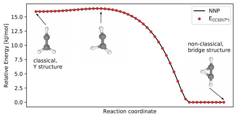
Figure 1: Energy profile along the minimum energy path (solid black line) as given by the global NN-PES of CCSD(T*) accuracy, see text. Along this path, single-point energies obtained by using the identical electronic structure method are shown as red dots for direct comparison. The global and local minimum of the C₂H${}_{3}^{+}$ molecule as well as the interconnecting saddle-point corresponding to the bridge, Y-shaped and transition state structures are depicted using ball-and-stick representations in the right, left and middle parts of the figure, respectively.

Multiple tests were performed to validate the accuracy of this NN-PES for protonated acetylene. This includes, among others discussed in the Supplementary Information, the calculation of the transition path between the bridged and Y-shaped conformations (using the improved tangent nudged elastic band method (NEB) method Henkelman and Jónsson (2000)) obtained from this NN-PES as presented in Fig. 1. Along this minimum energy path, a dense set of single-point energies was computed for comparison using the same CCSD(T*) methodology. The NN-PES is able to reproduce not only the 16.46 kJ/mol energy barrier of the rearrangement from the Y-shaped to the bridged isomer with essentially perfect agreement to the coupled cluster reference, but also the overall shape of the transition path including the extremely shallow local minimum of the Y-structure, such that the naked eye cannot recognize any difference on the intrinsic energy scale of that PES; we note in passing that this important energy pathway is consistent with the results reported earlier Psciuk, Benderskii, and Schlegel (2007). For comprehensive benchmarking, we refer to data obtained by evaluating the NN-PES in direct comparison to explicit single-point CCSD(T*) calculations (including energy predictions across the data set, important stationary-point energies, normal modes of the key minimum-energy structures, as well as potential energy scans along various internal generalized coordinates), which are compiled in Secs. I.A to D of the Supplementary Information. Overall, these tests confirm that the NN-PES fit is able to reproduce the coupled cluster PES of protonated acetylene very accurately.

This NN-PES was used to perform classical molecular dynamics (MD) and quantum path integral molecular dynamics (PIMD) simulations employing the CP2k simulation package cp (2); Hutter et al. (2014). In this context, we refer the interested reader to a recent review article Brieuc et al. (2020b) that unfolds the entire methodological framework that allows one to carry out converged quantum simulations of fluxional molecules or complexes even at cryochemical conditions. For the production runs, protonated acetylene was simulated at different temperatures ranging from 1 K to 1600 K using both, MD and PIMD simulations. In case of the PIMD simulations, the so-called PIQTB Brieuc, Dammak, and Hayoun (2016) thermostat as implemented by us in CP2k for usage down to ultra-low temperatures Schran, Brieuc, and Marx (2018) was utilized in order to converge the path integral in terms of its discretization. This Trotter convergence was examined in detail for simulations at 100 K and compared with the corresponding results obtained with standard canonical PIMD simulations using the so-called PILE Ceriotti et al. (2010) thermostat and a very large number of path integral replica. It was observed that in case of PIQTB using $P=48$ replica at 100 K is sufficient to provide converged results in terms of energetic as well as structural properties; see Sec. II in the Supplementary Information for details. It was also verified that both thermostats provide the same values of the quantity of interest, namely the interaction information $I_{n}$ up to 4-point correlations, as discussed in detail in Sec. II.C of the Supplementary Information. The number of replicas $P$ used for the simulations at different temperatures was determined as usual in such a way that the product $P\cdot T$ remains constant, thus providing similar relative discretizations at all temperatures, thus using $P=4\>800$ replica at our ultra-low temperature of 1 K. At very low temperatures, this approach was further validated by explicit benchmark simulations at 5 K where taking $P=960$ was shown to indeed provide converged results; we refer to Secs. II.A to B in the Supplementary Information for more details. All reported simulations were propagated for at least 2 ns in the case of PIMD simulations and at least for 82 ns for classical MD simulations. Overall, this adds up to a grand total of 2.2 $\upmu$s of classical and quantum simulations of protonated acetylene carried out at CCSD(T*) accuracy. A time step of 0.25 fs was used throughout and the first 2.5 ps of each simulation was discarded to account for thermalization.

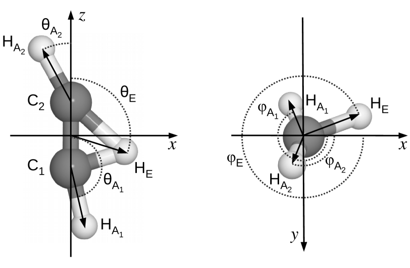
Figure 2: Definition of polar angles $(\theta_{\rm A_{1}},\theta_{\rm A_{2}},\theta_{\rm E})$, left panel, and azimuth angles $(\phi_{\rm A_{1}},\phi_{\rm A_{2}},\phi_{\rm E})$, right panel, used to describe the orientational configuration of the three protons with respect to the carbon atoms of the C₂H${}_{3}^{+}$ molecule. The corresponding distances of the axial and equatorial protons ($r_{\rm A_{1}},r_{\rm A_{2}},r_{\rm E}$) are not labeled in the figure but defined therein using arrows. All coordinates are defined with respect to a laboratory-fixed coordinate system as follows: The molecule is translated and rotated with respect to the $x$- and $z$-axes such that the two C atoms lie on the $z$-axis and that the origin is given by the C—C bond midpoint.

The structural correlation analysis was performed using a set of ten generalized coordinates of C₂H${}_{3}^{+}$, which are the C—C bond length ($r_{\rm CC}$), the C—H bond lengths of the two axial ($r_{\rm A_{1}},r_{\rm A_{2}}$) protons, the distance between the equatorial proton and the C—C midpoint ($r_{\rm E}$), the polar angles of each proton ($\theta_{\rm A_{1}},\theta_{\rm A_{2}}$ and $\theta_{\rm E}$) and the azimuth angles of each proton denoted as $\phi_{\rm A_{1}},\phi_{\rm A_{2}}$ and $\phi_{\rm E}$, respectively. This set of coordinates allows one to uniquely define all possible configurations of the protonated acetylene molecule within the laboratory-fixed coordinate system as defined in Fig. 2 together with the graphical definition of all ten coordinates. We note in passing that this set is very convenient for the present discussion but slightly redundant since only nine internal degrees of freedom exist for C₂H${}_{3}^{+}$. In case of the azimuth angles of the protons, $(\phi_{\rm A_{1}},\phi_{\rm A_{2}},\phi_{\rm E})$, periodic boundary conditions with a period of $2\pi$ apply. As a consequence, the distance between points $\phi_{i}$ and $\phi_{j}$ is given by

$$d_{\phi}(\phi_{1},\phi_{2})=\min\{|\phi_{i}-\phi_{j}|,2\pi-|\phi_{i}-\phi_{j}|\},$$

which can be easily generalized to higher dimensions.

By construction, our generalized coordinates are not invariant with respect to permutations, e.g. exchanging atoms H${}_{\rm A_{1}}$ with H_E changes the values of $r_{\rm A_{1}},r_{\rm E}$ and $\phi_{\rm A_{1}},\phi_{\rm E}$. In particular, these coordinates are only meaningful for bridge-like structures, see Fig. 1 for details. However, as evidenced by the minimum energy path in Fig. 1, the local minimum of the Y-configuration is extremely shallow with a barrier of only about 0.5 kJ/mol toward the global minimum, whereas the reverse barrier of the global minimum toward the Y-structure amounts to $\approx 16.5$ kJ/mol. Thus, the relative population of Y-like structures compared to bridge-like structures is expected to be overall very small at finite temperatures. In an effort to nevertheless take into account possible atom exchanges and thus permutations of axial versus equatorial proton labels when computing the respective generalized coordinates, we consider in each simulation step all possible permutations of the three H and two C nuclei (twelve permutations in total) according to that configuration and define a structure in a given permutation state to be bridge-like if the following set of conditions is fulfilled by the three polar angles: $3\pi/4\leq\theta_{\rm A_{1}}\leq\pi$, $0\leq\theta_{\rm A_{2}}\leq\pi/4$, and $\pi/2-0.6\leq\theta_{\rm E}\leq\pi/2+0.6$. These threshold values used to classify a given structure as bridge-like has been determined from the respective minima of the distribution functions of the polar angles when no permutations are applied as presented in Sec. III.A of the Supplementary Information. Modifying these threshold values in meaningful bounds only slightly impacts on the quantitative results, whereas the qualitative findings presented below remain unchanged. Indeed, explicit simulation shows that only very few structures, below 1 %, are in practice rejected by these criteria up to temperatures of 300 K, which is fully in line with the expected instability of Y-like structures given the shape of the interconversion profile Fig. 1.

Standard Nosé-Hoover-chain thermostatted molecular dynamics is used here to sample the classical canonical phase space distribution function at a given temperature, and thus to generate molecular structures in configuration space which are distributed according to the classical Boltzmann distribution. In the quantum case, path integral MD (PIMD) is correspondingly used to generate the configurations according to the canonical density matrix at the selected temperatures as detailed in Secs. II and III of the Supplementary Information. The internal coordinates are then constructed from these configurations and used as sample points for the computation of the associated entropies using the $k$-th NN estimator. In the PIMD case, the atomic positions of all replica were treated independently and the corresponding coordinates, computed for each replica separately, were added to the data set utilized to compute the $k$-th NN estimator, thus following the usual procedure to compute quantum expectation values of observables which are only defined in position space.

Prior to computing the $k$-th NN entropy estimator, values of all the coordinates, except the azimuth angles $\phi_{\rm A_{2}},\phi_{\rm A_{2}}$ and $\phi_{\rm E}$, are standardized so that they have the same standard deviation as the azimuth coordinates. This is done by subtracting the mean, dividing by the standard deviation of the given coordinate, and multiplying by the average standard deviation of azimuth coordinates. As already said, the interaction information according to Eq. (3) is invariant under such linear transformations, but in this way the effective distance scale between points in different dimensions is more homogeneous. This offers the numerical advantage that the convergence of the $k$-th NN entropy estimators is faster in higher dimensions.

In order to determine the distances $R_{i,k}$ required to compute the $k$-th nearest neighbor of all sample points, we used the ANN code ANN which utilizes the so-called “kd tree” algorithm Arya and Mount (1993a); Arya et al. (1998). Although with ANN it is possible to determine approximate nearest neighbors to reduce the computational complexity we decided to use here an exact algorithm instead ANN ; Arya and Mount (1993b).

The interaction information Eq. (3) can be estimated directly from the data Kraskov, Stögbauer, and Grassberger (2004), which usually provides a faster convergence with respect to the number of data points at a price of higher computational complexity. However, it turns out that, due to the high performance of NN-PES molecular dynamics simulations, it is computationally less demanding to generate large sets of uncorrelated structures and to use the $k$-th NN entropy estimator Eq. (4), combined with Eq. (3), than to estimate the interaction information directly from the data.

IV Results

In order to provide detailed insight into the correlations in fluxional molecules based on the above introduced configurational entropy analysis, we set out to study the temperature dependence of protonated acetylene, a prime candidate of large-amplitude motion and fluxionality. For that purpose, we performed exhaustive classical and quantum simulations spanning vastly different regimes: From ultra-low temperatures down to 1 K to ambient conditions to the highest temperature of 1600 K. The computational details of these simulations can be found in Sec. III with further references to the Supplementary Information. Concerning the convergence of the interaction information estimators with respect to number of data points we refer to Sec. III.B in the Supplementary Information. The resulting classical and quantum ensembles at these distinct temperatures enable the detailed analysis of the evolution of correlations as a function of temperature, while at the same time unraveling the importance of nuclear quantum effects in different temperature regimes.

To start the detailed configurational entropy analysis of correlations in protonated acetylene, all possible two-coordinate interaction informations for the ten coordinates presented in Fig. 2 were determined from the classical and quantum trajectories at several distinct temperatures. As an important first result, we observe that there are only three significant two-coordinate correlations. All other correlations are several times weaker and therefore will not be considered in the following. A detailed discussion of all correlations can be found in the Supplementary Information in Sec. IV.A, where we also show that the relative importance of the correlations neither depends on the temperature nor on treating the nuclei as classical or quantum point particles. The first prominent correlation, $I_{2}(r_{\rm E},\theta_{\rm E})$, is between the distance of the equatorial proton from the C—C bond, $r_{\rm E}$, and its polar angle $\theta_{\rm E}$. This is the only correlation that involves any of the existing bond lengths with protonated methane, i.e. all other correlations considered here, including the three- and four-coordinate ones, exclusively involve angular degrees of freedom. The second prominent correlation, $I_{2}(\theta_{\rm A_{1}},\theta_{\rm E})$ and its symmetry equivalent $I_{2}(\theta_{\rm A_{2}},\theta_{\rm E})$, involves the polar angle of one of the two axial protons (i.e. $\theta_{\rm A_{1}}$ or $\theta_{\rm A_{2}}$) and the polar angle of the equatorial proton $\theta_{\rm E}$. The last significant two-point correlation, $I_{2}(\phi_{\rm A_{1}},\phi_{\rm A_{2}})$, is observed between the azimuth angles of the two axial protons. Interestingly, the correlations between the azimuthal orientations of two axial protons is not mediated by the orbiting equatorial proton: Correlations between the variable $\phi_{\rm A_{1}}$ and any of three coordinates describing the position of the equatorial proton (i.e. $r_{\rm E},\theta_{\rm E},\phi_{\rm E}$) are always at least one order of magnitude weaker then $I_{2}(\phi_{\rm A_{1}},\phi_{\rm A_{2}})$. In fact, the interaction information between the azimuth angle of axial and equatorial protons, which seems to be a natural candidate to proxy the angular position of axial protons, is virtually zero, which proves that $\phi_{\rm A_{1}}$ and $\phi_{\rm E}$ are independent. In other words: Analysis of the two-point correlations suggests that the equatorial proton orbits around the molecular axis given by the C–C bond independently from the orientational arrangement of the two axial protons. However, the higher-order correlations paint a different picture as follows.

Let us next focus on the relevant higher-order correlations in protonated acetylene, while as before discussion of all correlations can be found in the SI in Sec. IV.B. There are only two significant three-coordinate correlations found which are in addition equivalent by symmetry: $I_{3}(\theta_{\rm E},\phi_{\rm A_{1}},\phi_{\rm E})$ and $I_{3}(\theta_{\rm E},\phi_{\rm A_{2}},\phi_{\rm E})$. They involve the two angular coordinates of the equatorial proton, namely the polar $\theta_{\rm E}$ and azimuth $\phi_{\rm E}$ angles, and the polar angle of one of the two axial protons, i.e. either $\phi_{\rm A_{1}}$ or $\phi_{\rm A_{2}}$. This result indicates that there exists a higher-order correlation between the orientations of the protons that cannot be explained by the respective two-coordinate correlations discussed above. In particular, no substantial two-coordinate correlations involving the $\phi_{\rm E}$ variable are recognized. Therefore, it can be concluded that the position of the orbiting equatorial proton is coupled in a non-trivial way to the arrangement of either one of the two axial protons and vice versa. Such a correlation has not been recognized previously Marx and Parrinello (1996); Knoll, Vager, and Marx (2003) due to the lack of appropriate analysis methodology. Notably, this three-coordinate correlation is found to be stronger than any of the two-coordinate correlations involving only angular coordinates and, therefore, cannot be interpreted as a minor correction only.

Among all possible four-coordinate correlations there is only the correlation given by $I_{4}(\theta_{\rm E},\phi_{\rm A_{1}},\phi_{\rm A_{2}},\phi_{\rm E})$ which is not negligible. However, the magnitude of $I_{4}$ is roughly half the value of $I_{3}$ and it features negative values in addition. This four-body correlation links the azimuth angles of all protons with the polar angle of the equatorial proton, hence connects only the coordinates that are present in the two three-coordinate correlations discussed in previous paragraph. This explains why the four-coordinate interaction information is negative. According to Eq. (3), its negative value can be interpreted as a redundancy in the information provided by the involved coordinates and usually indicates a common-cause relation between the involved variables. In our case this indicates that the azimuth position of the $\phi_{\rm A_{2}}$ coordinate is already partially determined by the values of $\theta_{\rm E},\phi_{\rm A_{1}}$ and $\phi_{\rm E}$ (an analogous relationship holds when $\phi_{\rm A_{2}}$ is replaced by $\phi_{\rm A_{1}}$ and vice versa).

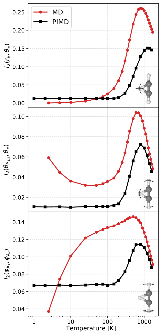
Figure 3: Significant two-coordinate correlations of protonated acetylene as a function of temperature: $I_{2}(r_{\rm E},\theta_{\rm E})$, $I_{2}(\theta_{\rm A_{1}},\theta_{\rm E})$ and its symmetry equivalent $I_{2}(\theta_{\rm A_{2}},\theta_{\rm E})$, as well as $I_{2}(\phi_{\rm A_{1}},\phi_{\rm A_{2}})$ from top to bottom. Correlations computed based on configurations generated using classical molecular dynamics (MD) simulations are marked using red lines, while the corresponding quantum path integral molecular dynamics (PIMD) data are given by black lines.

After having identified and discussed all relevant two-, three- and four-coordinate correlations in protonated acetylene, let us next focus on their temperature dependence and the impact of nuclear quantum effects. The temperature dependence of all significant two-coordinate correlations is presented in Fig. 3 whereas the important three- and four-point correlations are found in Fig. 4. We can clearly see that the results obtained from classical (MD) and quantum (PIMD) simulations differ considerably except in the limit of very high temperatures where the classical approximation approaches the quantum benchmark. As a first summary, it can be concluded that the correlations observed for classical nuclei are always stronger then those observed when quantum effects are included (except for obvious artifacts at sufficiently low temperatures where the classical approximation qualitatively fails to describe the system). This indicates that quantum delocalization tends to weaken the correlations over the whole temperature range studied here.

In the next step, we discuss the temperature evolution of the involved correlations in detail. We start by analyzing the classical results obtained from MD simulations. Generally speaking all correlations increase with temperature up to a certain point and then start to decay rapidly as temperature increases further. This trend holds true not only for the two-body correlations but is present in the many-body correlations as well, see Fig. 4 for three- and four-coordinate correlations. At low temperatures, classical dynamics pins the molecule close to its global minimum energy structure where it can only perform small-amplitude motion (mostly vibrations around that minimum energy structure). Upon increasing the temperature, correlations strengthen with reference to what is found at low temperatures, which can be understood in terms of increasing the PES landscape that becomes available to the system. As more thermal energy is provided, the system is able to explore larger regions of the PES such that more complex large-amplitude motions can unfold from which significant correlations are able to develop. In the high temperature limit, the relative importance of potential versus kinetic energy shifts toward the latter. Thus, the motion of the molecule is no longer strongly governed by the PES, but starts to be mostly a consequence of random thermal fluctuations. It is, thus, expected that further increase of the temperature will results in systematically decreasing correlations before, eventually, the molecule must fragment along particular dissociation channels which have not been considered in the present case.

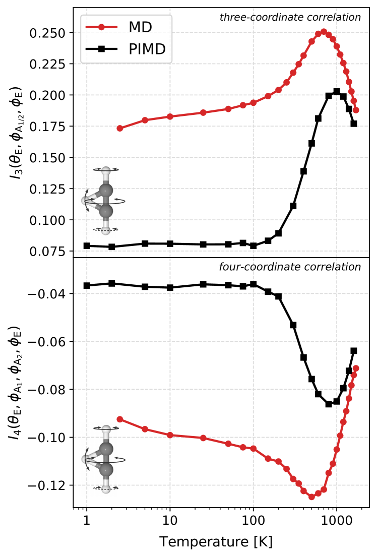
Figure 4: Significant three-coordinate (top) and four-coordinate (bottom) correlations of protonated acetylene as a function of temperature: $I_{3}(\theta_{\rm E},\phi_{\rm A_{1}},\phi_{\rm E})$ and its symmetry equivalent $I_{3}(\theta_{\rm E},\phi_{\rm A_{2}},\phi_{\rm E})$ as well as $I_{4}(\theta_{\rm E},\phi_{\rm A_{1}},\phi_{\rm A_{2}},\phi_{\rm E})$. Correlations computed based on configurations generated using classical molecular dynamics (MD) simulations are marked using red lines, while the corresponding quantum path integral molecular dynamics (PIMD) data are given by black lines.

In stark contrast to these classical results, the quantum simulations of protonated acetylene provide a completely different behavior for temperatures below 100 K, not only in terms of the estimated correlation strength but also in terms of the response to temperature changes. As can be seen in Fig. 3, the two-body correlations obtained from the quantum simulations are very small and, moreover, temperature independent below about 100 K. This observation also holds true for the higher-order correlations presented in Fig. 4. This combined analysis of all relevant correlations in protonated acetylene, thus, reveals the complete absence of any correlations in this temperature regime – if nuclear quantum effects are properly accounted for. At the same time, the classical correlations not only increase strongly with temperature, but also the estimated interaction information can be larger by two orders of magnitude compared to the low-temperature quantum limit.

In the quantum regime, protonated acetylene is essentially in its quantum ground state, thus quantum fluctuations play a dominant role whereas additional thermal activation effects are negligible. In other words: Classical simulations completely fail to correctly describe the correlations of protonated acetylene in the temperature regime below 100 K even at the qualitatively level. In this context, we draw attention to the fact that the $I_{2}(r_{\rm E},\theta_{\rm E})$ and $I_{2}(\phi_{\rm A_{1}},\phi_{\rm A_{2}})$ interaction information obtained from classical MD (Fig. 3) becomes even lower than its PIMD counterpart at these low temperatures. This effect is due to freezing out of the involved coordinates which is an unphysical artifact in view of the intrinsic zero-point vibrational motion even at 0 K.

For temperatures above approximately 800 K, however, protonated acetylene is reaching the classical regime where both classical and quantum simulations results start to be in quantitative agreement. This is exactly that temperature regime where the correlations, which initially increased upon heating, hit their maxima and thereafter systematically decay at even higher temperatures. That qualitative change in temperature response and, thus, disruptive behavior of all correlations within protonated acetylene is observed irrespective if the nuclei are treated as classical or quantum point particles. Although the classical simulations still overestimate the interaction information due to the neglect of quantum fluctuations, classical MD simulations can be used safely to study correlations of protonated acetylene in this regime.

Finally, for temperatures in between roughly 100 and 800 K a quantum-classical cross-over regime is observed in which the classical results are qualitatively in agreement with the quantum results, but the values of the correlations are heavily overestimated. At variance with low temperatures, quantum fluctuations are not dominant anymore in this regime as thermal fluctuations are becoming increasingly more important. For sufficiently large temperatures the quantum fluctuations are completely overwhelmed by thermal activation effects and the system enters the classical regime which is associated with the aforementioned bending of the curves at around 800 K.

The turning points, corresponding to the temperature at which a given correlation reaches its maximum value, is different in the classical and quantum treatment. It is observed that in case of quantum simulations these maxima are shifted towards higher temperatures by approximately 300 K. This phenomenon might be viewed as a remnant of quantum fluctuation effects that still contribute to the correlations.

Overall these results show the ability of the correlation analysis based on configurational entropy presented here to unravel complex correlated motion within fluxional molecules such as protonated acetylene. An important finding of this study is the striking difference between classical and quantum correlations highlighting the destructive character of quantum delocalization and zero point vibration that essentially destroy any correlations at low temperatures and, in particular, in the deep quantum regime. Even without knowing any details concerning the specific molecule, our entropy-based correlation analysis is able to uncover that the classical approximation to nuclear motion is entirely meaningless below about 100 K, while being qualitatively correct in between 100 and roughly 800 K and that it finally quantitatively describes protonated acetylene at temperatures of 1000 K and beyond.

V Conclusions and Outlook

In summary, we have outlined a systematic and rigorous analysis technique based on configurational entropy that allows one to quantify temperature-dependent structural correlations, both classical and quantum, within fluxional molecules. This general framework, which uses concepts originating in information theory, namely the non-parametric $k$-th nearest-neighbor configurational entropy estimation, can be used to decipher high-order correlations between any desired degrees of freedom without linearization or assumption of any parametric model. Applied to protonated acetylene C₂H${}_{3}^{+}$, an archetypal fluxional molecule, this analysis is able to unravel the intricate impact of temperature and nuclear quantum effects on intra-molecular structural correlations based on $n$-coordinate (a.k.a. $n$-body or $n$-point) interaction information estimators up to $n=4$.

Application to protonated acetylene shows that for our set of ten generalized coordinates chosen to characterize protonated acetylene, only three two-coordinate correlations have significant relevance for the complex configurational coupling in this molecule. In addition, two symmetry-equivalent three-coordinate correlations and a single four-coordinate correlation feature non-negligible magnitudes in the present case. Thus, protonated acetylene already provides a variety of correlation phenomena that go beyond the simple two-coordinate picture – as would be readily available using traditional covariance or principal component analyses based on the respective correlation coefficient matrix – although it certainly is a small molecule. This highlights that higher-order correlations significantly contribute to the overall complexity of the system and cannot be viewed as minor corrections.

Applying the technique to configuration ensembles that have been sampled from the classical and quantum canonical ensemble of the nuclear skeleton reveals three distinct temperature regimes as judged exclusively from inspecting the temperature-dependence of the $n$-body correlations. Below about 100 K the classical description of the nuclei provides unphysical artifacts whereas it works quantitatively correctly at temperatures of 1000 K or higher. In an intermediate regime from about 100 to 800 K, the quantum-to-classical cross-over occurs where classical nuclei fluctuating due to thermal activation qualitatively mimic the quantum-statistical description at the same temperature.

For classical nuclei, the obtained correlations start to increase continuously beyond roughly 100 K until reaching a maximum at about 800 K which is the temperature of the turnover to a rapid entropy-driven decay due to the overriding influence of the kinetic energy over the ordering effects of the potential energy. In contrast, we overall observe strongly reduced correlations for quantum nuclei, in particular at low temperatures due to quantum delocalization, which is prevailing for ground-state-dominated temperatures up to approximately 100 K. In the cross-over regime, the classical and quantum correlations are in qualitative agreement, albeit the latter are always much less pronounced than the former, and reach quantitative agreement only in the classical regime at the highest temperatures where thermal activation dominates.

This detailed data-intensive analysis has been made possible due to recent developments in machine learning approaches based on neural network representations of global potential energy surfaces in high dimensions, which allows us to describe the potential energy surface of protonated acetylene at the essentially converged coupled cluster level. This efficient and highly accurate approach enables the sampling of not only the classical, but also of the much more demanding quantum configurational ensemble in a statistically converged manner even at ultra-low temperatures close to the quantum ground state. Combining such sampling based on neural network potentials with the generic entropy-based scheme for determining high-order correlations in large-amplitude motion opens the door to study many other intricate molecules as well as inter-molecular correlations emerging in clusters or complexes.

References

References

- Kozachenko and Leonenko (1987) L. F. Kozachenko and N. N. Leonenko, “Sample estimate of the entropy of a random vector,” Probl. Inf. Transm. 23, 95–101 (1987).
- Singh et al. (2003) H. Singh, N. Misra, V. Hnizdo, A. Fedorowicz, and E. Demchuk, “Nearest neighbor estimates of entropy,” Amer. J. Math. Management Sci. 23, 301–321 (2003).
- Mnatsakanov et al. (2008) R. M. Mnatsakanov, N. Misra, S. Li, and E. J. Harner, “-nearest neighbor estimators of entropy,” Math. Methods Stat. 17, 261–277 (2008).
- Huggins (2014) D. J. Huggins, “Estimating translational and orientational entropies using the -nearest neighbors algorithm,” J. Chem. Theory Comput. 10, 3617–3625 (2014).
- Matsuda (2000) H. Matsuda, “Physical nature of higher-order mutual information: Intrinsic correlations and frustration,” Phys. Rev. E 62, 3096–3102 (2000).
- Killian, Yundenfreund Kravitz, and Gilson (2007) B. J. Killian, J. Yundenfreund Kravitz, and M. K. Gilson, “Extraction of configurational entropy from molecular simulations via an expansion approximation,” J. Chem. Phys. 127, 024107 (2007).
- Hnizdo et al. (2008) V. Hnizdo, J. Tan, B. J. Killian, and M. K. Gilson, “Efficient calculation of configurational entropy from molecular simulations by combining the mutual-information expansion and nearest-neighbor methods,” J. Comput. Chem. 29, 1605–1614 (2008).
- Karplus and Kushick (1981) M. Karplus and J. N. Kushick, “Method for estimating the configurational entropy of macromolecules,” Macromolecules 14, 325–332 (1981).
- Schlitter (1993) J. Schlitter, “Estimation of absolute and relative entropies of macromolecules using the covariance matrix,” Chem. Phys. Lett. 215, 617 – 621 (1993).
- Fenley et al. (2014) A. T. Fenley, B. J. Killian, V. Hnizdo, A. Fedorowicz, D. S. Sharp, and M. K. Gilson, “Correlation as a determinant of configurational entropy in supramolecular and protein systems,” J. Phys. Chem. B 118, 6447–6455 (2014).
- Fogolari et al. (2015) F. Fogolari, A. Corazza, S. Fortuna, M. A. Soler, B. VanSchouwen, G. Brancolini, S. Corni, G. Melacini, and G. Esposito, “Distance-based configurational entropy of proteins from molecular dynamics simulations,” PLOS ONE 10, 1–26 (2015).
- Huggins (2015) D. J. Huggins, “Quantifying the entropy of binding for water molecules in protein cavities by computing correlations,” Biophys J. 108, 928–936 (2015).
- Suárez and Díaz (2015) D. Suárez and N. Díaz, “Direct methods for computing single-molecule entropies from molecular simulations,” Wiley Interdiscip. Rev. Comput. Mol. Sci. 5, 1–26 (2015).
- Marx and Parrinello (1996) D. Marx and M. Parrinello, “The effect of quantum and thermal fluctuations on the structure of the floppy molecule C2H,” Science 271, 179 – 181 (1996).
- Knoll, Vager, and Marx (2003) L. Knoll, Z. Vager, and D. Marx, “Experimental versus simulated Coulomb-explosion images of flexible molecules: Structure of protonated acetylene ,” Phys. Rev. A 67, 022506 (2003).
- Psciuk, Benderskii, and Schlegel (2007) B. T. Psciuk, V. A. Benderskii, and H. B. Schlegel, “Protonated acetylene revisited,” Theor. Chem. Acc. 117, 75–80 (2007).
- Douberly et al. (2008) G. E. Douberly, A. M. Ricks, B. W. Ticknor, W. C. McKee, P. v. R. Schleyer, and M. A. Duncan, “Infrared photodissociation spectroscopy of protonated acetylene and its clusters,” J. Phys. Chem. A 112, 1897–1906 (2008).
- Fortenberry, Roueff, and Lee (2016) R. C. Fortenberry, E. Roueff, and T. J. Lee, “Inclusion of 13C and D in protonated acetylene,” Chem. Phys. Lett. 650, 126 – 129 (2016).
- Hariharan, Lathan, and Pople (1972) P. Hariharan, W. Lathan, and J. Pople, “Molecular orbital theory of simple carbonium ions,” Chem. Phys. Lett. 14, 385 – 388 (1972).
- Żurawski, Ahlrichs, and Kutzelnigg (1973) B. Żurawski, R. Ahlrichs, and W. Kutzelnigg, “Have the ions C2H and C2H classical or non-classical structure?” Chem. Phys. Lett. 21, 309 – 313 (1973).
- Vager et al. (1993) Z. Vager, T. Graber, E. P. Kanter, and D. Zajfman, “Direct observation of nuclear rearrangement in molecules,” Phys. Rev. Lett. 70, 3549–3552 (1993).
- Behler and Parrinello (2007) J. Behler and M. Parrinello, “Generalized neural-network representation of high-dimensional potential-energy surfaces,” Phys. Rev. Lett. 98, 146401 (2007).
- Behler (2014) J. Behler, “Representing potential energy surfaces by high-dimensional neural network potentials,” J. Phys.: Condens. Matter 26, 183001 (2014).
- Behler (2015) J. Behler, “Constructing high-dimensional neural network potentials: A tutorial review,” Int. J. Quantum Chem. 115, 1032–1050 (2015).
- Behler (2017) J. Behler, “First principles neural network potentials for reactive simulations of large molecular and condensed systems,” Angew. Chem. Int. Ed. 56, 12828–12840 (2017).
- Schran, Behler, and Marx (2020) C. Schran, J. Behler, and D. Marx, “Automated Fitting of Neural Network Potentials at Coupled Cluster Accuracy: Protonated Water Clusters as Testing Ground,” J. Chem. Theory Comput. 16, 88–99 (2020).
- Cover and Thomas (2006) T. M. Cover and J. A. Thomas, Elements of Information Theory, 2nd ed. (Wiley, 2006).
- Ohya and Petz (1993) M. Ohya and D. Petz, Quantum Entropy and Its Use (Springer, 1993).
- Henderson and Vedral (2001) L. Henderson and V. Vedral, “Classical, quantum and total correlations,” J. Phys. A: Math. Gen. 34, 6899–6905 (2001).
- Smith (2015) R. Smith, “A mutual information approach to calculating nonlinearity,” Stat 4, 291–303 (2015).
- McGill (1954) W. J. McGill, “Multivariate information transmission,” Psychometrika 19, 97–116 (1954).
- Timme et al. (2014) N. Timme, W. Alford, B. Flecker, and J. M. Beggs, “Synergy, redundancy, and multivariate information measures: an experimentalist’s perspective,” J. Comput. Neurosci. 36, 119–140 (2014).
- Hnizdo and Gilson (2010) V. Hnizdo and M. K. Gilson, “Thermodynamic and differential entropy under a change of variables,” Entropy 12(3), 578–590 (2010).
- Kraskov, Stögbauer, and Grassberger (2004) A. Kraskov, H. Stögbauer, and P. Grassberger, “Estimating mutual information,” Phys. Rev. E 69, 066138 (2004).
- Hnizdo et al. (2007) V. Hnizdo, E. Darian, A. Fedorowicz, E. Demchuk, S. Li, and H. Singh, “Nearest-neighbor nonparametric method for estimating the configurational entropy of complex molecules,” J. Comput. Chem. 28, 655–668 (2007).
- Duda, Hart, and Stork (2001) R. O. Duda, P. E. Hart, and D. G. Stork, Pattern Classification, 2nd ed. (Wiley, New York, 2001).
- Kung, Lin, and Kao (2012) Y.-H. Kung, P.-S. Lin, and C.-H. Kao, “An optimal -nearest neighbor for density estimation,” Stat. Probab. Lett. 82, 1786 – 1791 (2012).
- Efron and Tibshirani (1994) B. Efron and R. Tibshirani, An Introduction to the Bootstrap (New York: Chapman & Hall, 1994).
- Brieuc et al. (2020a) F. Brieuc, C. Schran, H. Forbert, and D. Marx, “RubNNet4MD: The RUB Neural Network for Molecular Dynamics Software Package Version 1,” (2020a), see https://www.theochem.rub.de/go/rubnnet4md.html.
- Adler, Knizia, and Werner (2007) T. B. Adler, G. Knizia, and H.-J. Werner, “A simple and efficient CCSD(T)-F12 approximation,” J. Chem. Phys 127, 221106 (2007).
- Knizia, Adler, and Werner (2009) G. Knizia, T. B. Adler, and H.-J. Werner, “Simplified CCSD(T)-F12 methods: Theory and benchmarks,” J. Chem. Phys. 130, 054104 (2009).
- Werner et al. (2019) H. J. Werner, P. J. Knowles, G. Knizia, F. R. Manby, M. Schütz, et al., “MOLPRO, version 2019.1, a package of ab initio programs,” (2019), see https://www.molpro.net.
- Henkelman and Jónsson (2000) G. Henkelman and H. Jónsson, “Improved tangent estimate in the nudged elastic band method for finding minimum energy paths and saddle points,” J. Chem. Phys. 113, 9978–9985 (2000).
- cp (2) CP2K, released under GPL license; 2019; freely available at https://www.cp2k.org.
- Hutter et al. (2014) J. Hutter, M. Iannuzzi, F. Schiffmann, and J. VandeVondele, “cp2k: atomistic simulations of condensed matter systems,” Wiley Interdiscip. Rev. Comput. Mol. Sci. 4, 15–25 (2014).
- Brieuc et al. (2020b) F. Brieuc, C. Schran, F. Uhl, H. Forbert, and D. Marx, “Converged quantum simulations of reactive solutes in superfluid helium: The Bochum perspective,” J. Chem. Phys. 152, 210901 (2020b).
- Brieuc, Dammak, and Hayoun (2016) F. Brieuc, H. Dammak, and M. Hayoun, “Quantum Thermal Bath for Path Integral Molecular Dynamics Simulation,” J. Chem. Theory Comput. 12, 1351–1359 (2016).
- Schran, Brieuc, and Marx (2018) C. Schran, F. Brieuc, and D. Marx, “Converged Colored Noise Path Integral Molecular Dynamics Study of the Zundel Cation Down to Ultralow Temperatures at Coupled Cluster Accuracy,” J. Chem. Theory Comput. 14, 5068–5078 (2018).
- Ceriotti et al. (2010) M. Ceriotti, M. Parrinello, T. E. Markland, and D. E. Manolopoulos, “Efficient stochastic thermostatting of path integral molecular dynamics,” J. Chem. Phys. 133, 124104 (2010).
- (50) ANN, released under GPL license; 2010; freely available at http://www.cs.umd.edu/~mount/ANN/.
- Arya and Mount (1993a) S. Arya and D. M. Mount, “Approximate nearest neighbor queries in fixed dimensions,” in Proceedings of the Fourth Annual ACM-SIAM Symposium on Discrete Algorithms, SODA ’93 (Society for Industrial and Applied Mathematics, USA, 1993) p. 271–280.
- Arya et al. (1998) S. Arya, D. M. Mount, N. S. Netanyahu, R. Silverman, and A. Y. Wu, “An optimal algorithm for approximate nearest neighbor searching fixed dimensions,” J. ACM 45, 891–923 (1998).
- Arya and Mount (1993b) S. Arya and D. M. Mount, “Algorithms for fast vector quantization,” in Proceedings of DCC’93: Data Compression Conference, edited by J. A. Storer and M.Cohn (IEEE Press, 1993) pp. 381–390.