Simultaneous compression and opacity data from time-series radiography
with a Lagrangian marker

Abstract

Time-resolved radiography can be used to obtain absolute shock Hugoniot states by simultaneously measuring at least two mechanical parameters of the shock, and this technique is particularly suitable for one-dimensional converging shocks where a single experiment probes a range of pressures as the converging shock strengthens. However, at sufficiently high pressures, the shocked material becomes hot enough that the x-ray opacity falls significantly. If the system includes a Lagrangian marker, such that the mass within the marker is known, this additional information can be used to constrain the opacity as well as the Hugoniot state. In the limit that the opacity changes only on shock heating, and not significantly on subsequent isentropic compression, the opacity of shocked material can be determined uniquely. More generally, it is necessary to assume the form of the variation of opacity with isentropic compression, or to introduce multiple marker layers. Alternatively, assuming either the equation of state or the opacity, the presence of a marker layer in such experiments enables the non-assumed property to be deduced more accurately than from the radiographic density reconstruction alone. An example analysis is shown for measurements of a converging shock wave in polystyrene, at the National Ignition Facility.

I Introduction

States of matter at elevated pressure and temperature are often generated in shock wave experiments shock , where the high-pressure matter is confined inertially (i.e. by the finite time required for the compressed components to disassemble) and so the pressures achieved are not limited by the strength of surrounding components as is the case with static presses dac . Material strength ranges up to $\sim$100 GPa, and the use of shock and other dynamic loading experiments is ubiquitous for high energy density studies of warm dense matter where pressures in excess of 1 TPa are of interest.

Large pulsed lasers such as the National Ignition Facility (NIF) NIF and Laboratory for Laser Energetics (omega laser, University of Rochester) OMEGA can be used to induce pressures in excess of 10 TPa, which are of interest for studies of massive exoplanets, brown dwarfs, and stars exoplanets ; Basri2006 ; Swift2012 ; Kirkpatrick2005 ; Arndt1998 , as well as engineering problems such as inertial confinement fusion (ICF) icf . We have previously reported the use of radiography of a spherically-converging shock to deduce a range of states along the shock Hugoniot of a material Kritcher2014 ; Doeppner2018 ; Swift2018 , up to $\sim$12 TPa in polystyrene, and thus to constrain the equation of state (EOS). The x-ray source was a foil, laser-heated to a plasma emitting strongly in the kilovolt regime. In the results reported previously, the shock temperature was low enough that the $K$-shell of the carbon atoms in the sample was not ionized significantly, which would have reduced the x-ray opacity and complicated the determination of mass density from the radiograph. However, at higher shock temperatures, the $K$-shell becomes significantly ionized. This ionization could occur at lower shock pressures if the initial mass density of the sample is lower, so this effect is relevant beyond the relatively high pressures considered here.

In the work reported here, we consider the use of a Lagrangian marker layer to constrain the mass enclosed, and hence enable the opacity to be deduced along with the mass density. The results reported here extend our previously-reported measurements Doeppner2018 ; Swift2018 to higher pressures, from experiments with a higher drive energy. This article describes the analysis procedure and results referred to in our recent article discussing the measurements and their relevance to white dwarf stars Kritcher2020 .

II Experimental configuration

The experimental configuration was as described previously Kritcher2014 ; Swift2018 ; Doeppner2018 , and is summarized here for convenience. The sample material was in the form of a solid sphere, surrounded by a shell of glow-discharge polymer (GDP) to act as an ablator, together referred to as the bead. The bead was mounted within a Au hohlraum hohlraum . With the exception of some beams used to generate x-rays for radiography, the remainder of the 192 beams of the NIF laser were used to heat the hohlraum and thus drive the bead. The hohlraum was filled with He to reduce the rate that ablated Au could permeate the hohlraum and impede the propagation of the laser beams. The resulting soft x-ray field within the hohlraum ablated the GDP, driving a shock into the bead. The overall configuration and laser pulses were based on ICF designs, to take advantage of synergies in fabrication and also the large development effort performed to give uniform drive conditions over the surface of the bead icf ; Kritcher2014 . (Fig. 1.)

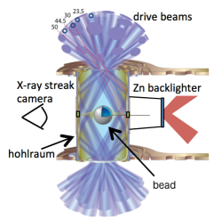
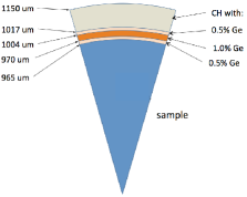
Figure 1: Schematic of hohlraum-driven converging-shock experiment. Wedge diagram shows sequence of shells comprising spherical target bead.

We consider data from two experiments, N130103-1 and N130701-1. In both cases, the sample was poly(alpha-methyl styrene) (PaMS), coated with a standard ICF ablator comprising GDP with a radially-varying concentration of Ge (Fig. 1) designed to absorb $M$-band radiation from the hohlraum. The hohlraum itself was Au, 30 $\mu$m thick, 5.75 mm diameter and 9.42 mm high. For commonality with the ICF campaign, the target in N130103-1 was cooled to 24 K, with a gas fill of 0.96 mg/cm³ He. When cooled, the initial mass density of the PaMS was calculated to be 1.13 g/cm³. Following changes to the allowed NIF experimental configurations, the target in N130701-1 was fired at ambient temperature, with a gas fill of 0.03 mg/cm³ He. The temporal shape of the laser pulses heating the hohlraum was based on ICF studies on the symmetric implosion of hollow capsules icf ; Hopkins2015 , which were designed to induce a pressure history in the ablator comprising a series of shocks to successively higher pressures. The pulse shape in N130103-1 induced four shocks, compared with two in N130701-1, again employing the most appropriate ICF configuration available at the time of each shot. With our solid sample, the shocks coalesced just within the sample to form a single, strong shock, so the precise pressure history induced in the ablator did not matter. The temperature history of soft x-rays in the hohlraum was calculated by radiation hydrodynamics using the hydra program hydra , and measured by the dante filtered diode system Dewald2004 . The peak temperature was around 275 eV.

The shock wave induced by ablation of the GDP strengthened as it propagated toward the center of the sample. X-ray radiography was used to measure the variation of attenuation across the diameter of the bead, from which the shock trajectory, mass distribution and opacity in the sample could be deduced as described below. The x-ray source was a Zn foil, driven by several laser beams to produce a plasma that emitted strong He-like radiation (i.e. from atoms stripped of all but two electrons). Eight beams were used in N130103-1, increased to sixteen in N130701-1 to increase the x-ray signal. Slits were cut in the hohlraum wall to enable transmission of the x-rays through the sample; the slits were filled with diamond wedges to impede their closure by ablated Au. The transmitted x-rays were imaged through a slit in a Ta foil onto an x-ray streak camera (Fig. 2).

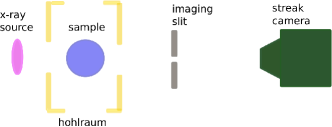
Figure 2: Radiograpic configuration (not to scale).

The streak radiograph was used to reconstruct the radial distribution of mass density, as a function of time. As described previously Swift2018 , the presence of undisturbed material ahead of the shock provided a strong constraint on the inference of the change in attenuation across the shock front. In order to take advantage of this constraint, the analysis was performed by adjusting a parameterized representation of the distribution of mass density until the corresponding simulated radiograph matched the measured radiograph. In the previous study, the change in attenuation was related directly to a change in mass density. At the higher pressures studied here, the change in attenuation was a combination of the change in mass density (increasing the attenuation) and in opacity (decreasing the attenuation).

Crucially for this experiment, the GDP ablator included a region doped with Ge, which was visible on the radiograph from shot N130103-1 (Fig. 3). As the mass inside the doped region is known, it provides an additional constraint that can be used to infer the opacity. In shot N130701-1, the lower hohlraum gas fill resulted in a higher intensity of Au $M$-band radiation, which was deposited in the doped region causing it to expand and lose contrast during the period covered by the radiograph (Fig. 4). As a result, the radiograph from shot N130103-1 was used to deduce the shock Hugoniot for cryogenic PaMS and its opacity as discussed below. The results were checked for consistency with the radiograph from shot N130701-1 and with hydrocode simulations.

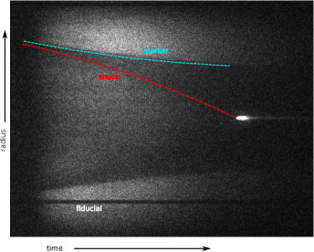
Figure 3: X-ray streak radiograph, NIF shot N130103-1 (cryogenic).

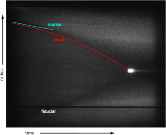
Figure 4: X-ray streak radiograph, NIF shot N130701-1 (ambient temperature).

Another interesting feature visible in the radiographs from experiments with high drive energies as here is a bright flash as the shock reached the center of the bead. Hydrodynamic heating was great enough for a region of the sample to radiate strongly enough in the kilovolt band to be detected by the streak camera. Radiation hydrodynamics simulations predicted x-ray intensities consistent with the radiographs Nilsen2018 , and the compact nature of the emitting region indicated the high degree of symmetry of the shock Bachmann2018 . (Figs 3 and 4.)

III Idealized simulations of the converging shock

As background for the analysis method developed, it is instructive to consider slightly idealized simulations of the converging shock in the sample. The simulations shown are one-dimensional Lagrangian in spherical geometry Benson1992 , for a shock propagating into a polystyrene sphere 2 mm in diameter, driven with a constant pressure of 8 TPa, which is representative of the ablation pressure in the NIF experiments. Polystyrene was represented by sesame EOS 7592 ses7592 . We consider the motion of Lagrangian tracers positioned initially at intervals of 100 $\mu$m through the sample.

As the shock passes, each tracer is accelerated toward the center, and the shock visibly accelerates as it nears the center (Fig. 5). The temperature history experienced by each tracer is a jump as the shock passes, followed by a more gradual increase on isentropic compression (Fig. 6). The mass density is in the range of several g/cm³, and the temperature from several tens to several hundred electron-volts. Under these conditions, widely-used atomic models imp ; opal ; atomic predict that the opacity should vary strongly with temperature, dropping by an order of magnitude as the shock pressure rises (Fig. 7).

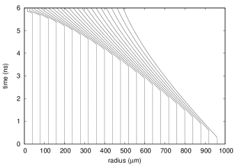
Figure 5: Motion of Lagrangian tracers in idealized simulation of spherically-converging shock.

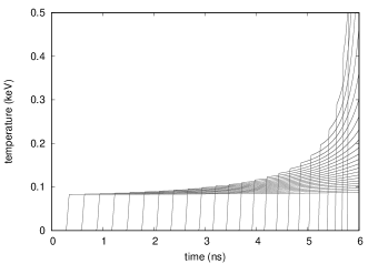
Figure 6: Temperature history of Lagrangian tracers in idealized simulation of spherically-converging shock.

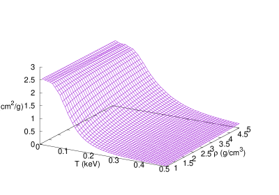
Figure 7: Opacity for polystyrene calculated using a model accounting for detailed configurations of excited electrons atomic .

When the shock temperature is sufficiently high, enough energy may be transported past the shock to heat the material ahead that the state induced by the shock may be significantly different than the principal Hugoniot. Using Lagrangian radiation hydrodynamics simulations with a variety of EOS and opacity models, we assessed the deviation in shock speed and mass density from thermal transport. We also assessed the change in opacity ahead of the shock, which could affect the inferred location of the shock in the radiograph. (Fig. 8.)

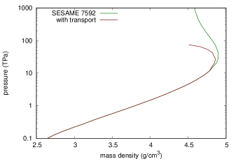
Figure 8: Sensitivity of inferred Hugoniot to heat transport ahead of the shock.

At the temperatures accessed in these converging-shock experiments, high enough to affect the x-ray opacity, for all but the lowest-$Z$ elements, the thermal energy of the electrons dominates over that of the ions, simply because there are more electrons in the system. Almost all wide-range EOS models have been constructed using the Thomas-Fermi (TF) approximation of a uniform electron gas tf , and so these EOS featured heavily in simulations used for sensitivity studies and for comparisons with experimental data, taken from the sesame and leos libraries sesame ; leos . A key question is whether the TF approximation, or variants, is adequate, or whether higher-order models treating electronic shell structure are necessary. The simplest form of shell structure treatment is the average atom model Liberman1979 ; Wilson2006 , which predicts pronounced features on the shock Hugoniot as successive electron shells are abruptly ionized; these predictions have been questioned as potentially exaggerating these ionization features in comparison with treatments including a more realistic distribution of atoms. Electron shell effects are important when constructing models of the opacity, which depends more sensitive than the EOS on accounting for the distribution of occupied and vacant electron states. As our analysis needs to use a model for off-Hugoniot variation of the opacity, we have used a range of specific opacity models, based on calculations from the imp imp , opal opal , and atomic atomic computer programs.

Radiation hydrodynamics simulations were used in this work to guide physical insight, design experiments, and test assumptions and analysis methods. These simulations typically bring together the state of the art in EOS, opacity, and numerical methods for continuum mechanics and radiation transport. No one person is fully aware of every aspect of all the models and methods. A notable benefit of exercising our simulation abilities on a new experimental platform like this has been to identify unexpected problems and limitations of models. For example, we discovered that one set of opacities tabulated for low-$Z$ materials was inaccurate for kilovolt photons because of an incorrect extrapolation at energies far above the binding energy of the $K$-shell. As well as being a useful finding in its own right, it highlights the value of designing experiments that can be interpreted as directly as possible from the measurements themselves, without being dominated by input from models or simulations. Even when measurements can be interpreted in this way, simulations may enter in a subtler way by informing the choice of initial conditions for iterative optimization of model parameters against the experimental data. Finally, the interplay between multiple physics models and implementations complicates the assessment of unexpected results, lengthening the process of turning experimental measurements into robust conclusions.

IV Determination of absolute Hugoniot and opacity data from radiography

As discussed previously Swift2018 , the reconstructed radius-time distribution of mass density $\rho(r,t)$ gives an absolute measurement of the shock Hugoniot over a range of pressures, from the position of the shock $r_{s}(t)$ and hence its speed $u_{s}(t)$, and the mass density immediately behind the shock, $\rho_{s}(t)=\rho(r_{s}(t),t)$. Simultaneous knowledge of $u_{s}$ and $\rho_{s}$ gives the complete mechanical state behind the shock by solving the Rankine-Hugoniot relations shock representing the conservation of mass, momentum, and energy across the shock,

$$u_{s}^{2} = v_{0}^{2}\displaystyle\frac{p-p_{0}}{v_{0}-v}$$ (1)

$$u_{p} = \sqrt{\left[(p-p_{0})(v_{0}-v)\right]}$$ (2)

$$e = e_{0}+\frac{1}{2}(p+p_{0})(v_{0}-v)$$ (3)

where $v$ is the reciprocal of the mass density $\rho$, $e$ is the specific internal energy, $p$ the pressure, and subscript ‘0’ denotes material ahead of the shock (with $u_{p}=0$). The state ahead of the shock is known, leaving five quantities to be determined ($v,p,e,u_{p},u_{s}$). If any two of these quantities are measured, the Rankine-Hugoniot equations determine the rest. In particular,

$$p=p_{0}+\displaystyle\frac{u_{s}^{2}}{v_{0}^{2}}\left(v_{0}-v\right).$$ (4)

Thus the mechanical state on the Hugoniot can be deduced directly from the distribution of mass density, without reference to any other material used as a standard, as is the case in some other experimental configurations, and so the measurement is absolute.

Given distributions of mass density $\rho(\vec{r},t)$ and opacity $\sigma(\vec{r},t)$ in the object, the signal along any path from the source $\vec{r}_{s}$ to the detector $\vec{r}_{d}$ at any instant of time is given by the integral of attenuation $\mu=\rho\sigma$ through the object,

$$I(\vec{r}_{d},t)=I(\vec{r}_{s})\exp\left[-\int_{\vec{r}_{s}}^{\vec{r}_{d}}\rho(\vec{r},t)\sigma(\vec{r},t)\,d\vec{r}\right]$$ (5)

neglecting scattering. If the opacity and density vary independently without further constraints, their variations cannot be separated. However, if the unknown opacity change occurs only along one locus, such as the shock front, and if the total visible mass is known, the variations can be separated from time-series data because, at each instant of time, the attenuation at the shock front and the difference between the total mass and the apparent mass provide two measurements from which the two unknowns can be deduced. The ‘visible mass’ may be defined with respect to a feature in the object that can be observed radiographically, to act as a Lagrangian marker. Suitable features include the interface between materials or a thin layer of material of different opacity.

This procedure works if there is only one unknown change in opacity between successive radiographic frames. For a converging shock, the compression changes behind the shock, with accompanying changes in temperature, which may lead to a change in the opacity. However, as discussed above, temperature change is dominated by the shock heating and this usually dominates the change in opacity, i.e. $\sigma(\chi,t)\simeq\sigma(\rho;\rho_{s})$. Changes caused by subsequent adiabatic heating can be ignored or accounted for with models of the opacity or opacity change.

Consider the radiograph as a map of the transmission through the object, $T(x,t)$, where $x$ is the space direction in the streak record. Neglecting scatter and the finite spatial resolution of the imaging system, the transmission at any point $(x,t)$ in the image is found from the integral through the object of the product of $\rho$ and the opacity $\sigma$,

$$T(x,t)=\exp\left[-\int\rho(r,t)\sigma(r,t)f(r,x)\,dr\right]$$ (6)

where $f(r,x)$ represents the geometrical mapping between radius within the object and position across the radiograph. Analogously to profile-matching of the distribution of mass density to match the radiograph when $\sigma$ is constant, for varying $\sigma$ we can instead use profile-matching to deduce the distribution of attenuation $\mu(r,t)\equiv\sigma(r,t)\rho(r,t)$. Although for the present experiment we are interested in spherical objects, the same approach can be applied to planar or cylindrical systems, so we will consider the generalized problem.

Suppose that at a given time $t_{2}$ in the streak radiograph, analysis of earlier data has given the mass density and opacity, $\{\rho,\sigma\}(r,t^{\prime}<t_{1})$. We define a Lagrangian ordinate $\chi$ with respect to a reference feature in the object (a marker layer or an edge) such that

$$\frac{d\chi}{dr}\propto r^{\alpha}\rho$$ (7)

where $\alpha$ is 0, 1, or 2 for planar, cylindrical, or spherical geometry. The mass enclosed by the feature is $M_{T}$, and the reference feature follows a trajectory $r_{r}(t)$. Given the instantaneous position of the shock $r_{s}(t)$, the mass of material outside the shock

$$M_{s}(t)\equiv\int_{r_{s}(t)}^{r_{r}(t)}\chi(r^{\prime},t)\,dr^{\prime}.$$ (8)

If the loading history experienced by each element of the sample is a shock followed by approximately isentropic loading or unloading, the opacity change is dominated by the amount of shock heating,

$$\sigma(\chi,t>t_{s}(\chi))=\sigma(\rho;\rho_{s}).$$ (9)

Considering the motion of the shock into initially undisturbed material between $t_{1}$ and $t_{2}=t_{1}+\delta t$, we want to deduce $\rho$ for the newly-shocked material. The first step is to analyze the attenuation $\mu(r,t_{2})$ to find the inner radius of material shocked up to $t_{1}$,

$$r_{1}(t_{2})\quad:\quad M_{1}=\int_{r_{1}}^{r_{r}}\frac{\mu(r,t_{2})}{\sigma(\chi(r^{\prime}))}\,dr^{\prime}.$$ (10)

If $\sigma$ is to vary with isentropic compression, the variation is included in the calculation of $r_{1}(t_{2})$, and the solution may become iterative. From the radius of the shock $r_{2}$ at $t_{2}$, the mass of unshocked material $M_{0}$, the mass density of the newly-shocked material is

$$\rho_{s}(t_{2})=\frac{M_{T}-[M_{0}(t_{2})+M_{1}(t_{2})]}{V(r_{1},r_{2};t_{2})}$$ (11)

where $V(r_{1},r_{2})$ is the volume enclosed between $r_{1}$ and $r_{2}$, which is proportional to $r_{2}^{\alpha}-r_{1}^{\alpha}$. Thus the opacity of the newly-shocked material

$$\sigma(\rho_{s})=\mu(r_{2},t_{2})/\rho_{s}.$$ (12)

This Lagrangian analysis also gives $r(\chi,t)$ from $\chi(r,t)$, and hence $u_{p}(\chi,t)$ and $u_{p}(r,t)$.

The equations above can be rewritten in differential form, but spatial integration from the marker layer is essential to finding the solution, so the problem has a fundamentally integro-differential character. Because the solution involves integration between the shock and the marker, error accumulates along the shock as the solution progresses, as with Abel inversion Abel1826 .

To summarize, the simultaneous reconstruction of mass density and opacity proceeds by performing profile-matching on the radiograph to determine the attenuation $\mu(r,t)$, identifying the trajectory of the shock and the marker, and applying the integral equations incrementally with time to reconstruct the motion of each element of material within the marker $r(\chi,t)$ and hence determine $\rho_{s}(t)$ and $\sigma_{s}(t)$.

For the previous analysis assuming constant opacity Swift2018 , several different methods were used to represent the radial variation of mass density through the shocked region, including a variety of functional forms and also tabulations with the ordinates typically distributed at uniform fractions of the separation between the shock and the marker. For the case of varying opacity, particularly when correcting for opacity variation with isentropic compression behind the shock, it was most efficient to construct the variation along lines of constant $\chi$ in the shocked region.

If the opacity changes only as the shock passes, it can be determined from the variation in the apparent mass enclosed by the marker.

$$\sigma_{0}\frac{dM}{dt}=4\pi r_{s}^{2}\rho_{0}u_{s}(\sigma_{s}-\sigma_{0})$$ (13)

therefore

$$\sigma_{s}=\sigma_{0}\left(1+\frac{dM/dt}{4\pi r_{s}^{2}\rho_{0}u_{s}}\right).$$ (14)

V Analysis of experimental data for poly(alpha methyl styrene) (PaMS)

In shot N130103-1, the doped layer in the ablator was visible throughout the duration of the radiograph, so the analysis described above could be performed to deduce the Hugoniot and opacity simultaneously. In addition, simpler analyses were performed to deduce the Hugoniot assuming a model for opacity, and also to deduce the opacity assuming a model for the EOS.

The streak radiograph was analyzed to deduce the radius-time distribution of mass density, represented using smooth functions as described previously Swift2018 . The analysis was performed in several different ways to gain confidence that the result did not depend on the choice of function. Alternative functions were used, and the analysis was performed over the full range of the streak record and also over shorter intervals of time.

The locus of the shock was represented by the function

$$r_{s}(t)=\alpha(t_{c}-t)^{\beta}$$ (15)

where $\alpha$, $\beta$, and $t_{c}$ were fitting parameters. The locus of the marker layer was represented by the function

$$r_{m}(t)=r_{\mbox{min}}+\alpha e^{-\beta t}$$ (16)

where $\alpha$, $\beta$, and $r_{\mbox{min}}$ were fitting parameters. These functions were able to capture these loci over the full range of the record. For shorter intervals, the same functions or polynomials were used.

The mass density in the shocked region was represented by interpolation between functions defined along the shock locus $\rho_{s}(t)$ and marker layer $\rho_{m}(t)$, with non-linear variation behind the shock represented either by functions defined along intermediate loci $\rho_{i}(t)$ or by analytically integrable functions

$$f(r,t)=\alpha(t)r^{2n}\exp\left[-r^{2}/2\sigma(t)^{2}\right],$$ (17)

The $\rho(t)$ functions and the time-dependent parameters $\alpha(t)$ and $\sigma(t)$ were represented using low-order polynomials or tabulations.

Given a reconstruction of the mass density, the Hugoniot was deduced from $\rho_{s}(t)$ and the shock speed, $-dr_{s}(t)/dt$. The goodness-of-fit of the simulated radiograph to the data was used to assign a probability to the model. By perturbing the fitting parameters about the best fit, Hugoniots were deduced with corresponding probability. The Hugoniot loci were accumulated as probability amplitudes. The nominal best-fitting Hugoniot was taken to be the locus of maximum likelihood, very similar to the Hugoniot from the best-fitting parameters, and 1$\sigma$ uncertainties were taken as contours from the probability distribution. These are the statistical fitting uncertainties. Systematic uncertainties from the uncertainty in instantaneous sweep rate of the streak camera and magnification affect the location of the Hugoniot, but affect its shape to a much smaller degree.

The uncertainty in opacity included an analogous, statistical contribution from fitting the radiograph. Since the opacity was deduced simultaneously with the reconstruction of mass density, the value along the locus of the shock can be associated with a statistically-exact Hugoniot state. The uncertainty in actual Hugoniot state associated an individual opacity has the same statistical and systematic uncertainties as the Hugoniot state itself, but these uncertainties are correlated exactly with the Hugoniot uncertainty. For this reason, we show only the statistical uncertainty in opacity.

V.1 Simultaneous Hugoniot and opacity analysis

The Hugoniot and opacity were deduced simultaneously, first by assuming that the opacity $\sigma$ changed only on passage of the shock, and then by assuming that its subsequent variation followed the local trend of an opacity model. Theoretical opacities are typically tabulated over mass density $\rho$, temperature $T$, and photon energy $E_{\gamma}$. An EOS is needed to deduce $T$ along the Hugoniot and for subsequent off-Hugoniot states. The effect of off-Hugoniot opacity variation is therefore an estimate depending on models of both opacity and EOS, and there is no a priori guarantee of consistency between the deduced Hugoniot and the EOS. Ideally, the analysis would be repeated with EOS adjusted as necessary to be consistent with the inferred Hugoniot, but such adjustment should also take account of data from other experiments, which is beyond the scope of the work reported here.

With the opacity assumed to vary only on passage of the shock, the deduced Hugoniot locus was softer (lower pressure for a given compression) than when the estimated off-Hugoniot opacity variation was included, and the opacity was deduced to drop more rapidly with pressure. For this assessment, we primarily used sesame EOS 7592 ses7592 and the opal opacity model opal . We also compared EOS states from a similar TF-based model, leos 5110 leos , illustrating variations typical of constructions by different individuals or using conventions and methods preferred by different research groups. (Figs 9 and 11.)

V.2 Hugoniot analysis assuming an opacity model

As with using a model to account for off-Hugoniot opacity variations, if the model is used also for the opacity on the Hugoniot, an EOS is also needed to deduce the temperature $T$. The deduced Hugoniot was similar to the result obtained above with opacity deduced from the radiograph and off-Hugoniot variations also accounted for, but with significantly smaller statistical uncertainty. (Figs 9 and 10.)

V.3 Opacity analysis assuming an equation of state

Conversely to the use of the radiograph to deduce the Hugoniot for an assumed opacity, it is possible to assume the EOS and deduce the opacity. For inconsistencies to be avoided, the EOS must be accurate enough to reproduce the locus of the shock given the locus of the marker layer to within the spatial resolution of the system. (Fig. 11.)

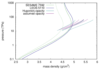
Figure 9: Hugoniot for PaMS with initial temperature 24 K, deduced from the high drive shot N130103 and compared with Thomas-Fermi based EOS. The dashed line is the sesame Hugoniot starting at STP, for comparison. Thin lines are $1\sigma$ contours for the corresponding thick line.

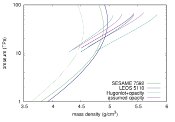
Figure 10: Hugoniot for PaMS with initial temperature 24 K, deduced from the high drive shot N130103 and compared with Thomas-Fermi based EOS. (Detail over range probed by these converging-shock experiments.)

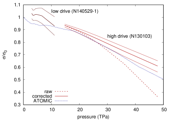
Figure 11: Opacity of PaMS to 9 keV x-rays. The nominal result for shot N130103-1 assumes that the opacity changes only on passage of the shock; the corrected curve uses EOS and opacity models to estimate the effect of isentropic compression. The result for the low-drive shot N140529-1 Doeppner2018 ; Swift2018 is also shown, consistent with a constant, cold opacity. Thin lines are $1\sigma$ contours for the corresponding thick line. The dotted line is the theoretical prediction from the atomic model atomic , with Hugoniot states from a recent average-atom EOS leos 5112 leos5112 .

V.4 Consistency with N130701-1

The early disappearance of the maker layer in shot N130701-1 means that the Hugoniot and opacity cannot be deduced simultaneously except at the lowest pressures sampled in the experiment. The duration of the x-ray pulse was longer than in N130103-1, covering a significantly greater range of shock radius and hence higher shock pressures and thus greater shock heating and a decreased opacity. Because N130701-1 was fired at ambient temperature, the initial mass density of the PaMS was 1.085 g/cm³ rather than 1.13 g/cm³ in N130103-1, and thus the Hugoniot pertaining to each experiment was slightly different. The effect of changing the initial density cannot be predicted from the Hugoniot measured at a single different density, but it can be estimated given off-Hugoniot information such as the Grüneisen parameter, which may be obtained from an existing EOS. Similarly, the opacity at the peak pressures reached in shot N130701-1 are not strictly constrained by the results of shot N130103-1, although the opacity at higher pressures can be estimated by extrapolation or use of a model.

At early time, while the marker was visible, the radiograph was analyzed as for N130103-1 for Hugoniot and opacity simultaneously. The opacity was consistent with cold material. The radiograph was therefore re-analyzed assuming the cold opacity, to give a section of the Hugoniot with smaller uncertainty (Fig. 12).

The radiograph was also analyzed by performing multiple one-dimensional hydrocode simulations, assuming a model of opacity, and adjusting the EOS until the residual in the simulated radiograph was minimized. The opacity model was constructed from the nominal opacity deduced from N130103-1 with off-Hugoniot variations taken from the opal model. The drive history was taken from radiation hydrodynamics predictions of the hohlraum temperature history, but was allowed to vary slightly to account for inaccuracies in hohlraum energetics and ablation modeling. Variations were introduced in the EOS in two ways: either the thermal contributions were held constant and parameters describing the cold compression curve were varied, or the cold curve was held constant and the thermal contributions were scaled by linear functions of mass density and temperature. Analogously with the treatment used when accumulating Hugoniot statistics from radiographic analysis, each simulation was assigned a likelihood from the difference in the simulated radiograph from the measurement, and the Hugoniot locus from the corresponding EOS was used to construct a probability distribution as a function of pressure and mass density. The nominal best-fitting Hugoniot was extracted as the peak locus in the distribution, along with $1\sigma$ contours for the distribution. As with N130103-1, these contours represent the statistical uncertainty, and are correlated relatively weakly with the systematic uncertainty from camera sweep rate and magnification. The resulting Hugoniot did depend significantly on the opacity model used, but was consistent with the Hugoniot estimated directly from N130103-1 with off-Hugoniot treatment from sesame 7592. The deduced Hugoniot was not sensitive to the EOS used as the basis for making variations. (Fig. 12.)

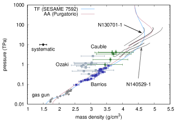
Figure 12: Ambient Hugoniot for PaMS. Thin lines are $1\sigma$ contours of statistical uncertainty from the parameterized fit to the radiograph. Systematic uncertainty from the uncertainty in magnification and the sweep speed of the x-ray streak camera is shown by the bar. Previous, planar, measurements Marsh1980 ; Cauble1998 ; Ozaki2009 ; Barrios2010 and the measurement from the low-drive spherical experiment N140529-1 Doeppner2018 are shown for comparison.

VI Conclusions

Time-resolved x-ray radiography of a one-dimensonal shock within a Lagrangian marker provides a way to deduce shock Hugoniot states simultaneously with the x-ray opacity. The Hugoniot measurement is absolute, i.e. without reference to an EOS standard, and can explore a range of states in a single experiment. For shocks driven by a laser-heated hohlraum, convergence can increase the pressure enough that the opacity decreases significantly as atoms in the sample are ionized. Convergence increased the shock pressure significantly over the externally-applied drive pressure without the drawbacks of increasing a driving radiation intensity, such as preheat.

Experiments on PaMS explored pressures of over 70 TPa, though absolute Hugoniot and opacity data were inferred only up to $\sim$40 TPa because of the loss of the marker layer in one experiment. The opacity inferred experimentally exhibited a decrease of similar magnitude over a similar range of temperatures to theoretical calculations including a detailed accounting of electron excitations.

References

- (1) For example, R.G. McQueen, S.P. Marsh, T.W. Taylor, J.N. Fritz, and W.J. Carter, in R. Kinslow (Ed.), “High Velocity Impact Phenomena” (Academic Press, New York, 1970).
- (2) For example, A.D. Chijioke, W.J. Nellis, A. Soldatov, and I.F. Silvera, The ruby pressure standard to 150 GPa, J. Appl. Phys. 98, 114905 (2005).
- (3) See National Technical Information Service Document No. DE2004-15007230 (E.I. Moses, introduction to the National Ignition Facility). Copies may be ordered from the National Technical Information Service, Springfield VA 22161.
- (4) See National Technical Information Service Document No. DE91013164 (University of Rochester report on Laboratory for Laser Energetics). Copies may be ordered from the National Technical Information Service, Springfield VA 22161.
- (5) J. Schneider and the Exoplanet Team, “The Extrasolar Planets Encyclopædia,” http://exoplanets.eu
- (6) G. Basri and M.E. Brown, Ann. Rev. Earth and Planet. Sci 34, 193-216 (2006).
- (7) D.C. Swift, J.H. Eggert, D.G. Hicks, S. Hamel, K. Caspersen, E. Schwegler, G.W. Collins, N. Nettelmann, and G.J. Ackland, Astrophys. J. 744, 59 (2012).
- (8) J.D. Kirkpatrick, Ann. Rev. Astron. and Astrophys. 43, 195-245 (2005).
- (9) S. Arndt, W. Däppen, A. Nayfonov, Astrophys. J. 498, 349-359 (1998).
- (10) J. Lindl, Phys. Plasmas 2, 3933 (1995).
- (11) A.L. Kritcher, T. Döppner, D. Swift, J. Hawreliak, G. Collins, J. Nilsen, B. Bachmann,E. Dewald, D. Strozzi, S. Felker, O.L. Landen, O. Jones, C. Thomas, J. Hammer, C. Keane, H.J. Lee, S.H. Glenzer, S. Rothman, D. Chapman, D. Kraus, P. Neumayer, and R.W. Falcone, High Energy Density Phys. 10, pp 27–34 (2014).
- (12) T. Döppner, D.C Swift, A.L Kritcher, B Bachmann, G.W Collins, D.A Chapman, J Hawreliak, D Kraus, J Nilsen, S Rothman, L.X Benedict, E Dewald, D.E Fratanduono, J.A Gaffney, S.H Glenzer, S Hamel, O.L Landen, H.J Lee, S LePape, T Ma, M.J MacDonald, A.G MacPhee, D Milathianaki, M Millot, P Neumayer, P.A Sterne, R Tommasini, and R.W Falcone, Phys. Rev. Lett. 121, 025001 (2018).
- (13) D.C. Swift, A.L Kritcher, J.A Hawreliak, A. Lazicki, A. MacPhee, B. Bachmann, T. Döppner, J. Nilsen, G.W Collins, S. Glenzer, S.D Rothman, D. Kraus, and R.W Falcone, Rev. Sci. Instrum. 89, 053505 (2018).
- (14) A.L. Kritcher, D.C. Swift, T. Döppner, B. Bachmann, L.X. Benedict, G.W. Collins, J.L. DuBois, F. Elsner, G. Fontaine, J.A. Gaffney, S. Hamel, A. Lazicki, W.R. Johnson, N. Kostinski, D. Kraus, M.J. MacDonald, B. Maddox, M.E. Martin, P. Neumayer, A. Nikroo, J. Nilsen, B.A. Remington, D. Saumon, P.A. Sterne, W. Sweet, A.A. Correa, H.D. Whitley, R.W. Falcone, and S.H. Glenzer, Nature 584, 7819, pp 51-54 (2020).
- (15) S.W. Haan, P.A. Amendt, T.R. Dittrich, B.A. Hammel, S.P. Hatchett, M.C. Herrmann, O.A. Hurricane, O.S. Jones, J.D. Lindl, M.M. Marinak, D. Munro, S.M. Pollaine, J.D. Salmonson, G.L. Strobel, and L.J. Suter, Nucl. Fusion 44, S171 (2004).
- (16) L.F. Berzak Hopkins, N.B. Meezan, S. Le Pape, L. Divol, A.J. Mackinnon, D.D. Ho, M. Hohenberger, O.S. Jones, G. Kyrala, J.L. Milovich, A. Pak, J.E. Ralph, J.S. Ross, L.R. Benedetti, J. Biener, R. Bionta, E. Bond, D. Bradley, J. Caggiano, D. Callahan, C. Cerjan, J. Church, D. Clark, T. Döppner, R. Dylla-Spears, M. Eckart, D. Edgell, J. Field, D.N. Fittinghoff, M. Gatu Johnson, G. Grim, N. Guler, S. Haan, A. Hamza, E.P. Hartouni, R. Hatarik, H.W. Herrmann, D. Hinkel, D. Hoover, H. Huang, N. Izumi, S. Khan, B. Kozioziemski, J. Kroll, T. Ma, A. MacPhee, J. McNaney, F. Merrill, J. Moody, A. Nikroo, P. Patel, H.F. Robey, J.R. Rygg, J. Sater, D. Sayre, M. Schneider, S. Sepke, M. Stadermann, W. Stoeffl, C. Thomas, R.P.J. Town, P.L. Volegov, C. Wild, C. Wilde, E. Woerner, C. Yeamans, B. Yoxall, J. Kilkenny, O.L. Landen, W. Hsing, and M.J. Edwards, Phys. Rev. Lett. 114, 175001 (2015).
- (17) M.M. Marinak, S.W. Haan, T.R. Dittrich, R.E. Tipton, and G.B. Zimmerman, Phys. Plasmas 5, 1125 (1998).
- (18) E.L. Dewald, K.M. Campbell, R.E. Turner, J.P. Holder, O.L. Landen, S.H. Glenzer, R.L. Kauffman, L.J. Suter, M. Landon, M. Rhodes, and D. Lee, Rev. Sci. Instrum. 75, 3759 (2004).
- (19) J. Nilsen, A.L. Kritcher, M.E. Martin, R.E. Tipton, H.D. Whitley, D.C. Swift, T. Döppner, B.L. Bachmann, A.E. Lazicki, N.B. Kostinski, B.R. Maddox, G.W. Collins, S.H. Glenzer, and R.W. Falcone, Matter and Radiation at Extremes 5, 1, 018401 (2020).
- (20) B. Bachmann et al (to be submitted).
- (21) D. Benson, Computer Methods in Appl. Mechanics and Eng. 99, 235 (1992).
- (22) J. Barnes and S. Lyon, documentation for sesame EOS 7592, unpublished (1988).
- (23) S.J. Rose, J. Phys. B: At. Mol. Opt. Phys. 25, 1667 (1992).
- (24) C.A. Iglesias, Astrophys. J. 464, 943 (1996).
- (25) P. Hakela, M.E. Sherrill, S. Mazevet, J. Abdallah Jr., J. Colgan, D.P. Kilcrease, N.H. Magee, C.J. Fontes, and H.L. Zhang, J. Quantitative Spectroscopy and Radiative Transfer 99, 265-271 (2006).
- (26) L.H. Thomas, Proc. Cambridge Phil. Soc. 23, 5, 542–548 (1927); E. Fermi, Rend. Accad. Naz. Lincei. 6, 602–607 (1927).
- (27) S.P. Lyon and J.D. Johnson, Los Alamos National Laboratory report LA-UR-92-3407 (1992).
- (28) R.M. More, K.H. Warren, D.A. Young and G.B. Zimmerman, Phys. Fluids 31, 3059 (1988); D.A. Young and E.M. Corey, J. Appl. Phys. 78, 3748 (1995).
- (29) D.A. Liberman, Phys. Rev. B 20, 12, 4981 (1979).
- (30) B. Wilson, V. Sonnad, P. Sterne, and W. Isaacs, J. Quant. Spectrosc. Radiat. Transfer 99, 658 (2006).
- (31) N.H. Abel, J. reine & angewandte Math., 1, pp. 153-157 (1826).
- (32) P. Sterne, Lawrence Livermore National Laboratory (unpublished).
- (33) S.P. Marsh (Ed), LASL Shock Hugoniot Data (University of California, Berkeley, 1980).
- (34) R. Cauble, T.S. Perry, D.R. Bach, K.S. Budil, B.A. Hammel, G.W. Collins, D.M. Gold, J. Dunn, P. Celliers, and L.B. Da Silva, Phys. Rev. Lett. 80, 1248 (1998).
- (35) N. Ozaki, T. Sano, M. Ikoma, K. Shigemori, T. Kimura, K. Miyanishi, T. Vinci, F.H. Ree, H. Azechi, T. Endo, Y. Hironaka, Y. Hori, A. Iwamoto, T. Kadono, H. Nagatomo, M. Nakai, T. Norimatsu, T. Okuchi, K. Otani, T. Sakaiya, K. Shimizu, A. Shiroshita, A. Sunahara, H. Takahashi, and R. Kodama, Phys. Plasmas 16, 062702 (2009).
- (36) M.A. Barrios, D.G. Hicks, T.R. Boehly, D.E. Fratanduono, J.H. Eggert, P.M. Celliers, G.W. Collins, and D.D. Meyerhofer, Phys. Plasmas 17, 056307 (2010).