Applying Lie Groups Approaches for Rigid Registration of Point Clouds
\autorLiliane Rodrigues de Almeida (1), Gilson A. Giraldi(1),
Marcelo Bernardes Vieira(2)
(1)Laboratório Nacional de Computação Científica
Petrópolis, RJ, Brasil.
lilianera@lncc.br , gilson@lncc.br
(2) Departamento de Ciência da Computação
Universidade Federal de Juiz de Fora
marcelo.bernardes@ufjf.edu.br
\setlrmarginsandblock3cm3cm*
\setulmarginsandblock3cm3cm*
\checkandfixthelayout
\SingleSpacing
[Abstract] In the last decades, some literature appeared using the Lie groups theory to solve problems in computer vision. On the other hand, Lie algebraic representations of the transformations therein were introduced to overcome the difficulties behind group structure by mapping the transformation groups to linear spaces. In this paper we focus on application of Lie groups and Lie algebras to find the rigid transformation that best register two surfaces represented by point clouds. The so called pairwise rigid registration can be formulated by comparing intrinsic second-order orientation tensors that encode local geometry. These tensors can be (locally) represented by symmetric non-negative definite matrices. In this paper we interpret the obtained tensor field as a multivariate normal model. So, we start with the fact that the space of Gaussians can be equipped with a Lie group structure, that is isomorphic to a subgroup of the upper triangular matrices. Consequently, the associated Lie algebra structure enables us to handle Gaussians, and consequently, to compare orientation tensors, with Euclidean operations. We apply this methodology to variants of the Iterative Closest Point (ICP), a known technique for pairwise registration. We compare the obtained results with the original implementations that apply the comparative tensor shape factor (CTSF), which is a similarity notion based on the eigenvalues of the orientation tensors. We notice that the similarity measure in tensor spaces directly derived from Lie’s approach is not invariant under rotations, which is a problem in terms of rigid registration. Despite of this, the performed computational experiments show promising results when embedding orientation tensor fields in Lie algebras.
Keywords: Rigid registration; Iterative Closest Point; Lie Groups, Lie Algebras, Orientation Tensors, CTSF.
1 Introduction
In computer vision application like robotics, augmented reality, photogrammetry, and pose estimation, the dynamical analysis can be formulated using transformation matrices as well as some kind of matrix operation [Zhang e Li 2014]. These ingredients comprise the elements of algebraic structures known as Lie groups, which are differentiable manifolds provided with an operation that satisfies group axioms and whose tangent space at the identity defines a Lie algebra [Huang et al. 2017]. One of the advantages of going from Lie group to Lie algebra is that we can replace the multiplicative structure to an equivalent vector space representation, which makes statistical learning methods and correlation calculation more rational and precise [Xu e Ma 2012].
Surface registration is a common problem in the mentioned applications [Berger et al. 2016], encompassing rigid registration that deals only with sets that differ by a rigid motion. In this case, given two point clouds, named source set , and target set , we need to find a motion transformation , composed by a rotation and a translation , that applied to best align both clouds (), according to a distance metric.
The classical and most cited algorithm in the literature to rigid registration is the Iterative Closest Point (ICP) [Besl e McKay 1992]. This algorithm takes as input the point clouds and , and consists of the iteration of two major steps: matching between the point clouds and transformation estimation. The matching searches the closest point in for every point in . This set of correspondences is used to estimate a rigid transformation. These two steps are iterated until a termination criterion is satisfied.
In order to compute the correspondence set, ICP and many other registration techniques use just the criterion of minimizing point-to-point Euclidean distances between the sets and . This approach might not be efficient in cases of partial overlapping, because only a subset of each point cloud has a correct correspondent instead of all the points. Local geometric features can be used to enhance the quality of the matching step. The key idea is to compute descriptors which efficiently encode the geometry of a region of the point cloud [Sharp, Lee e Wehe 2002]. Considering that we do not have triangular meshes representing the surfaces, we choose intrinsic elements that can be computed using the neighborhood of a point , that is represented by the list of its nearest-neighbors. Specifically, Cejnog [Cejnog, Yamada e Vieira 2017] proposed a combination between the ICP and the comparative tensor shape factor (ICP-CTSF) method that is based on second-order orientation tensors, computed using , which encodes the local geometry nearby the point . As in the focused application we have different viewpoints, with close perspectives of the same object, we expect that two correspondent points belonging to different viewpoints would have similar neighborhood disposition. Consequently, they are likely to have associated tensors with similar eigenvalues. This is the fundamental assumption in Cejnog’s work that has shown greatly enhancement in the matching step when combined with the closest point searching [Cejnog, Yamada e Vieira 2017].
More precisely, the above process generates two (discrete) tensor fields, say and . Given two points and the Cejnog’s assumption is based on the idea of computing a similarity measure between two symmetric tensors and by comparing their eigenvalues. Then, the similarity value is added to the Euclidean distance between and to get the correlation between them. Such viewpoint forwards some theoretical issues regarding tensor representation and metrics in the space of orientation tensors.
Given a smooth manifold of dimension , a tensor field can be formulated through the notion of tensor bundle which in turn is the set of pairs , where and is any tensor defined over . In terms of parametrization, it is straightforward to show that the tensor bundle can be covered by open sets that are isomorphic to open sets of where depends on and the tensor space dimension in each point [Renteln 2013]. In this sense, the tangent bundle is a differentiable manifold of dimension itself. Moreover, we can turn it into a Riemannian manifold by using a suitable metric which, for the purpose of statistical learning, can be the Fisher information one in the case of orientation tensors [Statistics, Skovgaard e (U.S.). 1981]. Therefore, we get the main assumption of this paper: compute matching step using the Riemannian structure behind the tensor bundle.
However, once orientation tensors can be represented by symmetric, non-negative definite matrices, we can embed our assumption in a multivariate Gaussian model and apply the methodology presented in [Li et al. 2017], which shows that the space of Gaussians can be equipped with a Lie group structure. The advantage of this viewpoint is that we can apply the corresponding Lie algebraic machinery which enables us to handle Gaussians (in our case, orientation tensors) with Euclidean operations rather than complicated Riemannian operations. More specifically, we show that the Frobenius norm in the Lie algebra of the orientation tensors over combines both the position of the points and the local geometry.
In this study, we focus on the ICP-CTSF and the combination between the Shape-based Weighting Covariance ICP and the CTSF, named SWC-ICP [Yamada et al. 2018]. We keep the core of each algorithm and insert in the matching step the Frobenius norm in the Lie space. In the tests, we analyze the focused techniques against fundamental issues in registration methods [Salvi et al. 2007, Tam et al. 2013, Díez et al. 2015]. Firstly, some of them, like ICP, assume that there is a correct correspondence between the points of both clouds. This assumption easily fails on real applications because, in general, the acquired data is noisy and we need to scan the object from multiple directions, due to self-occlusion as well as limited sensor range, producing only partially overlapped point clouds. Another issue of ICP and some variants is that they expect that the point clouds are already coarsely aligned. Besides, missing data is a frequent problem, particularly when using depth data, due uncertainty caused by reflections in the acquisition process.
To evaluate each algorithm in the target application, we consider point clouds acquired through a Cyberware 3030 MS scanner [Cyberware 1999] available in the Stanford scanning repository [Levoy et al. 1994]. The Bunny model was chosen for the tests. We take the original data and generate multiple case-studies, through a rigid transformation, addition of noise and missing data. In this case, the ground truth rotation and translation are available and, as a consequence, we can measure the errors without ambiguities.
The remainder of this paper is organized as follows. Section 2, we summarize the considered registration methods as well as the traditional ICP to set the background for rigid registration. Next, section 3 describes basic concepts in Lie groups and Lie algebras. The technique for embedding Gaussian models in linear spaces (named DE-LogE) is revised in 4. The corresponding logarithm expression is analyzed in more details in section 5. Next, section 6 discuss the comparison between orientation tensors in the associated Lie algebra while section 7 analyses the influence of rigid transformations. The section 8 shows the experimental results obtained by applying DE-LogE in the registration methods to point clouds. Section 9 presents the conclusions and future researches.
2 Registration Algorithms
We apply in this work two different algorithms to rigid registration: ICP-CTSF [Cejnog, Yamada e Vieira 2017] and SWC-ICP [Yamada 2016] In this section, we aim to establish the necessary notation and the mathematical formulation behind these techniques.
Hence, the bold uppercase symbols represent tensor objects, such as ; the normal uppercase symbols represent matrices, data sets and subspaces (, , , , etc.); the bold lowercase symbols denotes vectors (represented by column arrays) such as , . The normal lowercase symbols are used to represent functions as well as scalar numbers (, , , etc.). Also, given a matrix and a set , then is the trace of , and means the number of elements of . Besides, represents the identity matrix.
Our focus is rigid registration problem in point clouds. So, let the source and target point clouds in represented, respectively, by and . A rigid transformation is given by:
| (1) |
with and being the rotation matrix and translation vector, respectively.
The registration problem aims at finding a rigid transformation that brings set as close as possible to set in terms of a designated set distance, computed using a suitable metric , usually the Euclidean one denoted by . To solve this task, the first step is to compute the matching relation that denotes the set of all correspondence pairs to be used as input in the procedure to compute the transformation . Formally, we consider:
| (2) |
In the remaining text we are assuming that .
However, we must consider cases with only partial matches. Therefore, it is desirable a trimmed approach that discards a percentage of the worst matches [Chetverikov et al. 2002]. So, we sort the pairs of the set such that and consider a trimming parameter and a trimming boolean function:
| (3) |
So, we can build a new correspondence relation as:
| (4) |
which is supposed to have . We must notice that if .
The relationship defined by the expression (4) is based on the distance function and nearest neighbor computation. We could also consider shape descriptors computed over each point cloud. Generally speaking, given a point cloud , the shape descriptors can be formulated as a function , where is the set of all subsets of , named the power set of . In this case, besides the distance criterion, we can also include shape information in the correspondence computation by applying a boolean correspondence function such that [Díez et al. 2015]:
| (5) |
Also, before building in expression (2) we could perform a down-sampling in the two point sets, based on the selection of key points through the shape function, or through a naive interlaced sampling over same spatial data structure [Li et al. 2011].
Anyway, at the end of the matching process we get a base of the set , denoted by , and a base of the set , denoted by such that stands for the set of correspondence pairs . This matching relation will be used to estimate a rigid transformation that aligns the point clouds and . Specifically, we seek for a rotation matrix and a translation that minimizes the mean squared error:
| (6) |
which is used as a measure of the distance between the target set and the transformed source point cloud , with defined by equation (1). Now, we focus in the specific three-dimensional case () and state the fundamental theorem that steers most of the solutions for the registration problem in .
Theorem 1.
Let and , the centers of mass , for the respective point sets and , the cross-covariance , and the matrices and , given by:
| (7) |
| (8) |
| (9) |
| (10) |
| (11) |
Hence, the optimum rotation and translation t vector that minimizes the error in expression (6) are determined uniquely as follows [Horn 1987]. The matrix is computed through the unit eigenvector of , corresponding to its maximum eigenvalue:
| (12) |
and is calculated through and centroids in expressions (7)-(8) as:
| (13) |
2.1 Iterative Closest Point
The classical ICP [Besl e McKay 1992], described in the Algorithm 1, receives the source and target point clouds and it is composed by two major steps, iterated until a stopping criterion is satisfied, usually the number of iterations or error threshold.
2.2 ICP-CTSF
The ICP-CTSF [Cejnog, Yamada e Vieira 2017] implements a matching strategy using a feature invariant to rigid transformations, based on the shape of second-order orientation tensors associated to each point. A voting algorithm is used, divided into an isotropic and an anisotropic voting field. So, given a cloud point , let be the set of nearest neighbor of and . We can define , , as well as the function:
| (14) |
where is farthest neighbor of , which has influence . Given these elements, we can compute the second-order tensor field:
| (15) |
which is the isotropic voting field computed through a weighted sum of tensors , built from the function (14) and from the vote vectors , .
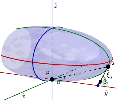
Let the orthonormal basis generated by the eigenvectors of and the corresponding eigenvalues supposed to satisfy . In this case, the local geometry at the point can be represented by the Figure 1 where we picture together the following elements: the coordinate system define by the eigenvectors , the plane that contains the point and the axis , its neighbor , and the ellipse that is tangent to the plane in and is centered at . The vector , that is unitary and tangent to at , gives a way to build a different structuring element that enhances coplanar structures in the sense that the angle if is close to the plane. Specifically, if is the arc length from to as indicated in the Figure 1, we define a new weighting function:
| (16) |
where is calculated by expression (14), is the angle between and the plane, constrains the influence of points misaligned to the plane, with an ideal choice, as a mid term between smoother results and robustness to outliers [Vieira et al. 2004].
With the above elements in mind, it is defined the tensor field , that is composed by the weighted sum of the tensors built from the votes received on the point, with weights computed by expression (16) for all the points that have as a neighbor:
| (17) |
The tensor field in expression (17) can be seen as a shape function whose descriptors at a point are the eigenvalues Therefore, given two points such that and , we compare the corresponding (local) geometries using the comparative tensor shape factor (CTSF), defined as:
| (18) |
where and are tensors computed following expression (17) and and are the th eigenvalues calculated in the points and , respectively.
The CTSF is used side by side with the Euclidean distance to produce a correspondence set that takes into account not only the nearest point (like in expression (2)) but also the shape information:
| (19) |
where is given by Equation (18), , with , and .
The parameter is the initial weight given to the CTSF and controls the update size of the weighting factor. To avoid numerical instabilities we set , when . This weighting strategy is responsible for its coarse-to-fine behavior when inserted in the matching step of the ICP algorithm, given by expression (2). Specifically, the ICP-CTSF procedure (Algorithm 2) calculates the correspondence relation:
| (20) |
and uses it to define the set:
| (21) |
which is the correspondence set applied by the ICP-CTSF technique, which is summarized in the Algorithm 2.
2.3 SWC-ICP Technique
In this technique, besides the correspondence relation (2), we also use the correspondence set:
| (22) |
which contains the pairs of points whose local shapes are the most similar, according to the criterion calculated by expression (18). In order to combine both the correspondence sets, we firstly develop expression (9) to get:
| (23) |
So, if we take expression (6) and perform the substitution:
| (24) |
with , we can write the mean squared error (6) as:
| (25) |
Also, by substituting the variable change (24) in expression (7) we get:
| (26) |
and, consequently:
| (27) |
where is computed by equation (8). We shall notice that the matrix (27) combines the matching relations (2) and (22) being fundamental for the SWC-ICP described in [Yamada 2016]. According to the Theorem 1, the optimum rotation matrix and translation vector t that minimizes the error in expression (25) are uniquely determined by equations (12)-(13) where is the unit eigenvector of corresponding to the maximum eigenvalue. However, the SWC-ICP methodology achieves a coarse-to-fine behavior through the use of the weighting strategy of the ICP-CTSF. The SWC-ICP technique can be summarized in the Algorithm 3.
3 Lie Groups and Lie Algebras
In this section we present some results and concepts of Lie groups theory that are relevant to problems in computer vision. We start with the tensor product operation which allows to define tensors and tensor fields. Next, we present the topological space definition which relies only upon set theory. This concept gives the support to define a differentiable manifold. The latter when integrated with the algebraic structure of groups yields the framework of Lie groups.
3.1 Tensor Product Spaces
The simplest way to define the tensor product of two vector spaces and , with dimensions and , is by creating new vector spaces analogously to multiplication of integers. For instance if and are basis in and , respectively, then, the tensor product between these spaces, denoted by , is a vector space that has the following properties:
-
1.
Dimension:
(28) -
2.
Basis:
(29) -
3.
Tensor product of vectors (Multilinear): Given and we define:
(30)
Generically, given vector spaces , such that , and is a basis for , we can define:
| (31) |
and the properties above can be generalized in a straightforward way.
3.2 Topological Spaces
Given a set we denote by the set of the parts of which is given by:
| (32) |
A topology over is a set that
fulfills the following axioms [Honig 1976]:
e1) Let an index set. If then the
union satisfies
e2) is such
that
e3)
The pair is called a topological space.
The elements of are called points and the elements of
are called open sets. A subset is named closed if its
complement is open.
We must remember that:
and so, the empty set must belong to
Given a point , we call a neighborhood of any set that contains an open set such that A topological space is separated or Hausdorff if every two distinct points have disjoint neighborhoods; that is, if given any distinct points there are neighborhoods and such that
It is possible to define the concept of continuity in topological spaces. Given two topological spaces and a function we say that is continuous in a point if there is a neighborhood such that
3.3 Differentiable Manifolds and Tensors
Let be a Hausdorff space as defined in section 3.2. A differential structure of dimension on is a family of one-to-one functions , where is an open set of and is an open set of , such that:
1)
2) For every the mapping is a differentiable function.
A differentiable manifold of dimension , denoted by , is a Hausdorff space with a differential structure of dimension for which the family is maximal respect to properties (1) e (2). If we replace differentiable to smooth in property (2) then is called a smooth manifold.
The family is an atlas on the topological space and each pair is named a chart.
Let and . Then, the set gives a local coordinate system in and are the local coordinates of .
Let be a smooth curve in the manifold , parameterized as In local coordinates the curve is defined by smooth functions of the real variable Let the point of for . Then, the tangent vector at in is given by the derivative:
The tangent vector to at can be expressed in the local coordinates as:
| (33) |
where and the vectors are defined by the local coordinates.
So, we can define the tangent space to a manifold at a point as:
| (34) |
We can show that is a vector space, isomorphic to . Besides, the set:
| (35) |
gives a natural basis for .
The collection of all tangent spaces to is the tangent bundle of the differentiable manifold
| (36) |
A Riemannian manifold is a manifold equipped with an inner product in each point (bilinear form in the tangent space ) that varies smoothly from point to point. A geodesic in a Riemannian manifold is a differentiable curve that is the shortest path between any two points and (see [Boothby 1975]).
A vector field over a manifold is a function that associates to each point a vector . Therefore, in the local coordinates:
| (37) |
where now we explicit the fact that expressions (33) and (35) are computed in each point .
The notion of tensor field is formulated as a generalization of the vector field using the concept of tensor product of section 3.1. So, given the subspaces , with , , the tensor product of these spaces, denoted by , is a vector space defined by expression (31) with and individual basis ; that means, a natural basis for the vector space is the set:
| (38) |
In this context, a tensor of order in is defined as an element that is, an abstract algebraic entity that can be expressed as [Liu e Ruan 2011]:
| (39) |
Analogously to the vector case, a tensor field of order over a manifold is a function that associates to each point a tensor . On the other hand, analogously to the tangent bundle, we can define the tensor bundle as:
| (40) |
where we shall notice that if .
3.4 Group Definition
A group is a pair where is a non-empy set and is a mapping, also called an operation [Lang 1984], with the following properties:
(1) Associative. If , then:
(2) Unity element. There is an element , named unit element, such that:
for all
(3) Inverse. For any there exists an element , called inverse, that satisfies:
A commutative (or abelian) groups satisfies:
| (41) |
Examples of Abelian Groups: and
, where ’’ is the usual addition.
Matrix Groups: Let be the real matrices. We shall consider the usual matrix multiplication . In this case, we can show that the following subsets of are groups regarding matrix multiplication.
2) : real matrices with non-null determinant
4) : the set of upper triangular matrices with positive diagonal entries
5) or : symmetric positive definite matrices
7) : the group of matrices with positive determinant
3.5 Lie Groups and Lie Algebras
An Lie group is a group and also a differentiable manifold of dimension such that the group operation [Olver 1986]:
and inversion:
are smooth functions.
Examples:
(a) Let with the trivial differential structure given by the identity mapping and the usual addition operation in , where the inverse of a vector is its opposite Once both the addition and inversion are smooth mappings, is an example of a r-parametric Lie group.
(b) Consider the set composed by the rotations:
with the usual matrix multiplication. It is straightforward to show that the group axioms are satisfied and, consequently, os a group. Its differential structure can be obtained by the observation that we can identify with the unitary circle [Olver 1986]:
and, consequently, is a Lie group.
Let and two Lie groups. A homeomorphism between these groups is a smooth function that satisfies:
Besides, if is bijective and its inverse is smooth, we say that is an isomorphism between and .
If then the tangent space at satisfies . Moreover, the Lie Algebra associated to the group is the vector space . Hence, considering the definition (34) of tangent space, we see that for all we have:
| (42) |
| (43) |
where This fact motivates the following definition.
Definition 1: Let G be a matrix Lie group. The Lie algebra of G, denoted as , is the set of all matrices such that for all real numbers . Therefore:
is a curve in the group . It is straightforward to show that this curve satisfies the properties (42)-(43). Besides the matrix exponential is a function that can be computed by the series:
| (44) |
For and , let:
which is an open disc of radius in . So, we can show that the function [Baker 2002]:
| (45) |
is well-defined and we can prove that .
4 Embedding Gaussians into Linear Spaces
In this section we summarize some fundamental results presented in [Li et al. 2017]. So, we consider the spaces:
-
1.
: Space of Gaussians of dimension . Each Gaussian distribution is denoted by , where is the mean vector and the covariance matrix
-
2.
: The set of all upper triangular matrices
-
3.
: symmetric matrices
Let and the Cholesky decomposition , where is a lower triangular matrix with positive diagonal. Steered by this decomposition, we can define the following operation in .
| (46) |
Theorem 3.
Under the operation given by expression (46), the set is a Lie group, denoted by
Now, let us consider the Lie group :
where the operation ’’ is the usual matrix multiplication.
Theorem 4.
The function given by:
where and , is an isomorphism between the Lie groups and .
Dem: [Li et al. 2017].
Now, we take the set:
which is the Lie algebra of the matrix group .
Theorem 5.
The function given by:
is a smooth bijection and its inverse is smooth as well.
Dem: [Li et al. 2017].
Theorem 6.
Log-Euclidean on ): We define the operation:
and:
Under the operation , is a commutative Lie group. Besides:
is a Lie group isomorphism. In addition, under and , is a linear space.
Dem: [Li et al. 2017].
Consequently, we can complete an embedding process, denoted by DE-LogE in [Li et al. 2017], as:
where and . Recall that is the Cholesky factor of .
5 Studying the DE-LogE
Let us denote:
| (47) |
Therefore, according to expression (45), if we can write:
| (48) |
Just as a prospective example, we are going to analyse the above Taylor expansion for :
We shall notice that:
where .
Consequently:
where:
| (49) |
| (50) |
The pattern observed in equations (49)-(50) is verified for all . To demonstrate this, it is just a matter to notice that:
| (51) |
Consequently, using an induction process, if we assume that:
where:
| (52) |
| (53) |
then:
Using equation (51) we obtain:
and, consequently:
which concludes the induction process.
Consequently, we can compute the function:
which is well defined if [Baker 2002], and write:
where
| (54) |
| (55) |
6 Comparing Tensors in DE-LogE
Therefore, from expressions (54)-(55), given matrices and in the form of expression (47), we can compute the difference:
| (56) |
So the matrix encompasses two kinds of non-null elements; the first one that holds the Cholesky decomposition of the tensors:
| (57) |
and the second one where the coordinates of the points and explicitly appear:
| (58) |
We follow the ICP-CTSF philosophy and assume that the points corresponding to the same region in two different point clouds have similar shape tensors because their surrounding geometry are the same. Hence in expression (57) should be low. However, we shall include the distance between points in order to avoid convergence to local minimum. Expression (58) can be used to solve this problem once it includes the positions of the points and . Therefore, we can compare the geometries nearby points and using the square of Frobenius norm in LogE space:
| (59) |
or a variant which includes a weight to distinguish the influence of each term:
| (60) |
However, before going ahead we must analyse the influence of rotations and translations in the above expressions.
7 Effect of Rigid Transformations
We consider the rigid transformation:
| (61) |
and the perfect alignment where . So, we can compute the second-order tensor field defined by expression (15) in the target cloud :
| (62) |
Hence, given and , we also have: and and . Like in section 2.2, we define , compute its normalized version:
| (63) |
and the function:
| (64) |
once is an orthogonal matrix. However, from expressions (61) and (64) we obtain:
| (65) |
Moreover:
consequently:
| (66) |
Regarding the Cholesky decomposition , we can write:
| (67) |
where is a lower triangular matrix.
Therefore, under rigid transformation and the DE-LogE embedding process becomes:
| (68) |
So, given and we obtain:
| (69) |
In this case, the ideal situation would be , where . However, we can not guarantee this property because in general. As a consequence, we can not guarantee invariance to rotations for which is a problem for registration algorithms.
8 Experimental Results
Despite of the difficulties regarding the non-invariance of against rotations, we present in this section some tests to evaluate expressions (59)-(60) in rigid transformation tasks. Specifically, we keep the strategy of expression (19) and put together the Euclidean distances and shape features by applying expressions (59) and (60) instead of (19), generating two strategies:
- 0.
- 1.
Hence, we compare the alignment given by the methods ICP-CTSF and SWC-ICP, and their variants using the Lie algebra, named ICP-LIE-0 and SWC-LIE-0 (case 0 above), ICP-LIE-1 and SWC-LIE-1 (case 1 above). The two input point clouds are obtained by sampling the Bunny model, from the Stanford 3D Scanning Repository [Levoy et al. 1994], based on the selection of key points at a fixed step. For the following experiments, this step is chosen to be , resulting in a set of points. The source point cloud corresponds to the target point cloud, but rotated by counterclockwise over the vertical axis, and no translation is added (Figures 2.(i)-(ii) ). With this setup, we have the ground truth transformation and point-by-point correspondence. The registration algorithms are compared by using root mean squared error (), computed by:
| (70) |
where is given by equation (6) and the pair is the rotation and translation (respectively) obtained through the registration process.
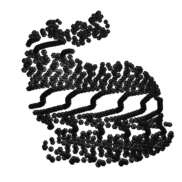
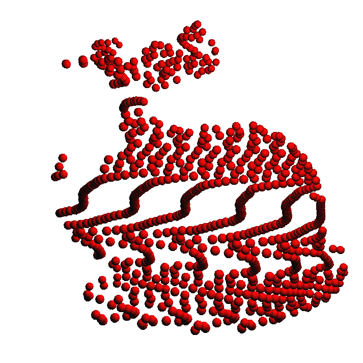
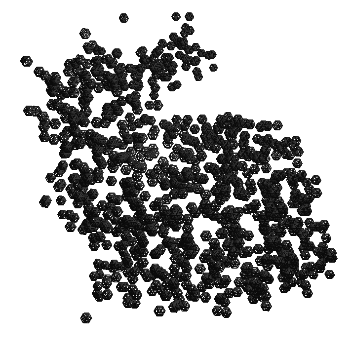
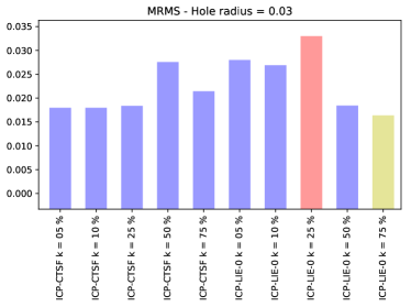
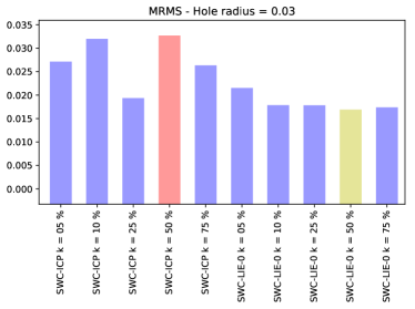
Besides the point clouds in Figures 2.(i)-(ii) , we take the Bunny model configuration and build a case-study for registration under missing data by moving it using the same rotation and translation as before. Then, we remove a set of points inside a ball centered in a specific point in the cloud, with , and update the correspondence set (see Figures 2.(iii)-(iv)). The last scenario is composed by the original clouds corrupted by noise. Noise is simulated adding to each point a vector , where is a random normalized isotropic vector, is a Gaussian random variable with null mean and variance equals to , and denotes a scale factor. Specifically, if denotes a generic point in the set (or ) then its corrupted version is , given by: . The new point sets, denoted by and , are composed by the noisy points so generated. We experiment with to generate the noisy clouds and , which are pictured on Figures 2.(v)-(vi).

(i) (ii)
(ii)
(iii)
 (iv)
(iv)

(v)
 (vi)
(vi)
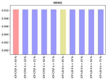
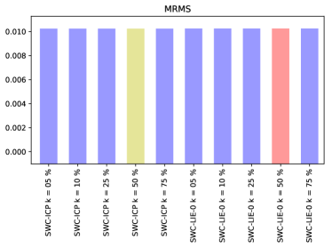
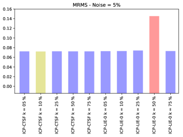
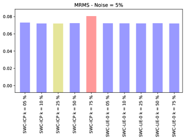
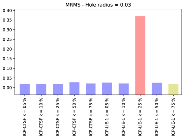
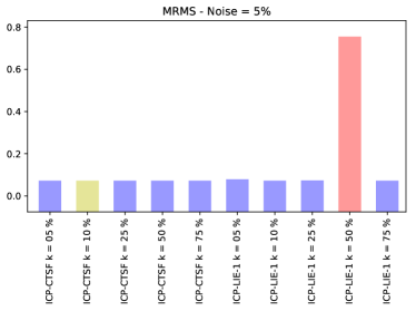
Figures 3.(a)-(f) allow to compare the focused techniques when applied to register clouds in Figure 2. These plots report the of ICP-CTSF and SWC-ICP procedures (Algorithms 2-3) according to the ground truth correspondence, as well as the of each technique obtained when using strategies above.
(a)
 (b)
(b)
(c)
 (d)
(d)
(e)
 (f)
(f)
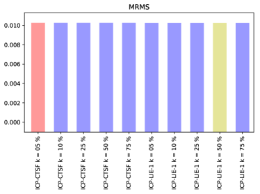
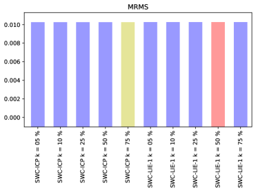
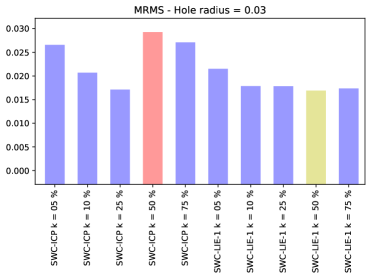
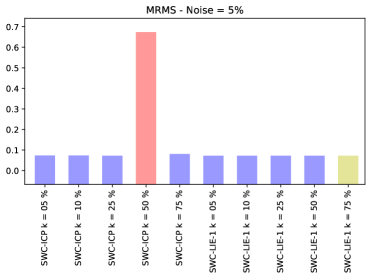
Next, Figures 4.(a)-(f) present the analogous results but using ICP-CTSF and SWC-ICP, together with their Lie versions obtained by replacing expression (19) to equation (60) with defined likewise in Algorithms 2-3.
(a)
 (b)
(b)
(c)
 (d)
(d)
(e)
 (f)
(f)
The Table 1 summarizes the results shown in Figures 3-4. We notice that the Lie approaches perform better than the traditional ICP-CTSF and SWC-ICP for original clouds and in the presence of missing data (hole). However, in the scenario containing noise the ICP-CTSF outperforms all the other approaches.
| Strategies | Scenario | Best ICP | Best SWC | Best |
| 0 | Original | ICP-LIE-0, | SWC-ICP, | 0.010257717275893 |
| Hole | ICP-LIE-0, | SWC-LIE-0, | 0.016357583571102 | |
| Noise | ICP-CTSF, | SWC-ICP, | 0.071996330253377 | |
| 1 | Original | ICP-LIE-1, | SWC-ICP, | 0.010257717275893 |
| Hole | ICP-LIE-1, | SWC-LIE-1, | 0.016911773470017 | |
| Noise | ICP-CTSF, | SWC-LIE-1, | 0.071996330253377 |
9 Conclusion and Future Works
In this paper we consider the pairwise rigid registration of point clouds. We take two techniques, named by the acronyms ICP-CTSF and SWC-ICP, and apply a Lie algebra framework to compute similarity measures used in the matching step. We use point clouds with known ground truth transformations which allows to compare the new techniques with their original implementations. The results show that the of Lie approaches are better than traditional ones for original clouds and in the presence of missing data but the traditional ICP-CTSF outperforms Lie techniques for noisy data. Further works must be undertaken to improve ICP-LIE and SWC-LIE and to bypass the non-invariance of DE-LogE against rotations.
References
- [Baker 2002] BAKER, A. Matrix Groups: An Introduction to Lie Group Theory. London, UK: Springer, 2002. (Springer undergraduate mathematics series).
- [Berger et al. 2016] BERGER, M. et al. A survey of surface reconstruction from point clouds. In: WILEY ONLINE LIBRARY. Computer Graphics Forum. [S.l.], 2016.
- [Besl e McKay 1992] BESL, P. J.; MCKAY, N. D. A method for registration of 3-d shapes. IEEE Trans. Pattern Anal. Mach. Intell., IEEE Computer Society, Washington, DC, USA, v. 14, n. 2, p. 239–256, fev. 1992. ISSN 0162-8828.
- [Boothby 1975] BOOTHBY, W. An Introduction to Differentiable Manifolds and Riemannian Geometry. Elsevier Science, 1975. (Pure and Applied Mathematics). ISBN 9780080873794. Disponível em: aetemad.iut.ac.ir/sites/aetemad.iut.ac.ir/files//files_course/william_m._boothby_an_introduction_to_differentibookfi.org_.pdf.
- [Cejnog, Yamada e Vieira 2017] CEJNOG, L. W. X.; YAMADA, F. A. A.; VIEIRA, M. B. Wide angle rigid registration using a comparative tensor shape factor. International Journal of Image and Graphics, v. 17, n. 01, p. 1750006, 2017.
- [Chetverikov et al. 2002] CHETVERIKOV, D. et al. The trimmed iterative closest point algorithm. In: IEEE. Pattern Recognition, 2002. Proceedings. 16th International Conference on. [S.l.], 2002. v. 3, p. 545–548.
- [Cyberware 1999] CYBERWARE. Cyberware 3030 MS scanner. [s.n.], 1999. Disponível em: http://cyberware.com/products/scanners/3030.html.
- [Díez et al. 2015] DÍEZ, Y. et al. A qualitative review on 3d coarse registration methods. ACM Computing Surveys (CSUR), ACM, v. 47, n. 3, p. 45, 2015.
- [Honig 1976] HONIG, C. S. Alicacoes da Topologia a Analise. [S.l.]: Editora Edgar Blucher, Ltda, SP-Brasil, 1976.
- [Horn 1987] HORN, B. K. Closed-form solution of absolute orientation using unit quaternions. JOSA A, Optical Society of America, v. 4, n. 4, p. 629–642, 1987.
- [Huang et al. 2017] HUANG, Z. et al. Deep learning on lie groups for skeleton-based action recognition. 2017 IEEE Conference on Computer Vision and Pattern Recognition (CVPR), p. 1243–1252, 2017.
- [Lang 1984] LANG, S. Algebra. Yale University, New Haven: Addison-Wesley Pub. Company, Inc., 1984.
- [Levoy et al. 1994] LEVOY, M. et al. Bunny Model. https://graphics.stanford.edu/data/3Dscanrep/: [s.n.], 1994.
- [Li et al. 2011] LI, C. et al. Fast and robust isotropic scaling iterative closest point algorithm. In: 18th IEEE International Conference on Image Processing, ICIP 2011, Brussels, Belgium, September 11-14, 2011. [S.l.: s.n.], 2011. p. 1485–1488.
- [Li et al. 2017] LI, P. et al. Local log-euclidean multivariate gaussian descriptor and its application to image classification. IEEE Transactions on Pattern Analysis and Machine Intelligence, v. 39, p. 803–817, 2017.
- [Liu e Ruan 2011] LIU, S.; RUAN, Q. Orthogonal tensor neighborhood preserving embedding for facial expression recognition. Pattern Recognition, v. 44, n. 7, p. 1497 – 1513, 2011.
- [Olver 1986] OLVER, P. J. Applications of Lie Groups to Differential Equations. [S.l.]: Springer-Verlag, Berlin, (1986), 1986.
- [Renteln 2013] RENTELN, P. Manifolds, tensors and forms: An introduction for mathematicians and physicists. [S.l.]: Cambridge University Press, 2013.
- [Salvi et al. 2007] SALVI, J. et al. A review of recent range image registration methods with accuracy evaluation. Image and Vision Computing, Elsevier, v. 25, n. 5, p. 578–596, 2007.
- [Sharp, Lee e Wehe 2002] SHARP, G. C.; LEE, S. W.; WEHE, D. K. Icp registration using invariant features. Pattern Analysis and Machine Intelligence, IEEE Transactions on, IEEE, v. 24, n. 1, p. 90–102, 2002.
- [Statistics, Skovgaard e (U.S.). 1981] STATISTICS, S. U. D. of; SKOVGAARD, L.; (U.S.)., N. S. F. A Riemannian Geometry of the Multivariate Normal Model. Statistical Research Unit, 1981. Disponível em: https://books.google.com.br/books?id=VQpfGwAACAAJ.
- [Tam et al. 2013] TAM, G. et al. Registration of 3d point clouds and meshes: A survey from rigid to nonrigid. Visualization and Computer Graphics, IEEE Transactions on, v. 19, n. 7, p. 1199–1217, 2013. ISSN 1077-2626.
- [Vieira et al. 2004] VIEIRA, M. B. et al. Smooth surface reconstruction using tensor fields as structuring elements. In: WILEY ONLINE LIBRARY. Computer Graphics Forum. [S.l.], 2004. v. 23, n. 4, p. 813–823.
- [Xu e Ma 2012] XU, Q.; MA, D. Applications of lie groups and lie algebra to computer vision: A brief survey. 2012 International Conference on Systems and Informatics (ICSAI2012), p. 2024–2029, 2012.
- [Yamada et al. 2018] YAMADA, F. A. et al. Comparing seven methodogies for rigid alignment of point clouds with focus on frame-to-frame registration in depth sequences. SBC Journal on Interactive Systems, v. 9, n. 2, p. 82–104, 2018.
- [Yamada 2016] YAMADA, F. A. de A. A shape-based strategy applied to the covariance estimation on the ICP. Dissertação (Mestrado) — Post-Graduation Program on Computer Science, Federal University of Juiz de Fora, Juiz de Fora, MG, Brazil, 2016.
- [Zhang e Li 2014] ZHANG, B.; LI, Y. F. Automatic Calibration and Reconstruction for Active Vision Systems. [S.l.]: Springer Publishing Company, Incorporated, 2014. ISBN 9401781001, 9789401781008.