MANTRA: A Machine Learning reference lightcurve dataset for astronomical transient event recognition

Abstract

We introduce MANTRA, an annotated dataset of $4869$ transient and $71207$ non-transient object lightcurves built from the Catalina Real Time Transient Survey. We provide public access to this dataset as a plain text file to facilitate standardized quantitative comparison of astronomical transient event recognition algorithms. Some of the classes included in the dataset are: supernovae, cataclysmic variables, active galactic nuclei, high proper motion stars, blazars and flares. As an example of the tasks that can be performed on the dataset we experiment with multiple data pre-processing methods, feature selection techniques and popular machine learning algorithms (Support Vector Machines, Random Forests and Neural Networks). We assess quantitative performance in two classification tasks: binary (transient/non-transient) and eight-class classification. The best performing algorithm in both tasks is the Random Forest Classifier. It achieves an F1-score of $96.25\%$ in the binary classification and $52.79\%$ in the eight-class classification. For the eight-class classification, non-transients ($96.83\%$) is the class with the highest F1-score, while the lowest corresponds to high-proper-motion stars ($16.79\%$); for supernovae it achieves a value of $54.57\%$, close to the average across classes. The next release of MANTRA includes images and benchmarks with deep learning models.

1 Introduction

Large scale automatic detection and classification of astronomical transients is happening within surveys such as Pan-STARRS1 (Kaiser, 2004), the Palomar Transient Factory (Law et al., 2009), the Catalina Real-Time Transient Survey (Drake et al., 2009), the All-Sky Automated Survey for SuperNovae (Shappee et al., 2014) and the Zwicky Transient Factory (Bellm et al., 2019). Besides the large amount of data, transient classification is hard because the data is usually heterogeneous, unbalanced, sparse, unevenly sampled and with missing information.

These two characteristics (size and heterogeneity) have motivated the application of Machine Learning (ML) algorithms to face this challenge. For instance, Random Forests, MultiLayer Perceptron and K-Nearest Neighbours have been used on lightcurves to classify transients from the Catalina Real Time Transient Survey (D’Isanto et al., 2016); convolutional neural networks have been used as input to automatic vetting algorithms (quick classification of bogus vs. real transients) based on data from the SkyMapper Supernova and Transient Survey and the High cadence Transient Survey (HiTS) (Gieseke et al., 2017; Cabrera-Vives et al., 2017).

The quality of the dataset is a necessary, although insufficient, requirement for the success of these examples and of any other ML implementation. New ML results usually come from groups internal to an observational collaboration because they have the internal know-how (and, sometimes, privileged access) to build training datasets. Consequently, despite having a lot of data available in the public domain, much of it is difficult to access. This difference in data access makes it challenging for the broader astronomical and machine learning communities to rebuild a training dataset, perform comparisons with published results and suggest new algorithms.

Other collaborations have directly published large datasets of simulated transients hoping to trigger more involvement from the ML in astronomy community at large to develop new classification algorithms (The PLAsTiCC team et al., 2018). However, at the time of writing, no dataset for transients has been made accessible to the public in the form of a catalogue based on real data.

To this end we compile and publish in easy-to-access files a dataset that can be used to train and test different ML algorithms for transient classification. We use public data from the Catalina Real-Time Transient Survey (CRTS) (Drake et al., 2012), an astronomical survey searching transient and highly variable objects as base for the dataset. Effectively, we developed an ETL (Extract, Transform and Load) procedure to extract the data from CRTS, which is designed for a sporadic lookup of a few objects, into a catalogue of thousands of objects that can be used to train ML algorithms and establish benchmarks. Here, in the first paper, we present the lightcurve data. In a second paper we will present a curated imaging dataset from the same survey.

This paper is structured as follows. In Section 2 we present the CRTS and the steps we follow to build the dataset. Then, in Section 3 we describe its main features together with the repository structure gathering the files and Python code to explore it. In Section 4 we show how this dataset can be used to perform tests using ML methods following a similar approach as D’Isanto et al. (2016), and the experiments that we perform. We finalize in Section 5 with a summary of the main features of our dataset and the results of our experiments.

2 The lightcurve dataset

We use public data from the Catalina Real-Time Transient Survey (CRTS) (Drake et al., 2009; Mahabal et al., 2011), an astronomical survey searching transient and highly variable objects. The CRTS covered 33000 squared degrees of sky and took data since 2007. Three telescopes were used: Mt. Lemmon Survey (MLS), Catalina Sky Survey (CSS), and Siding Spring Survey (SSS). So far, CRTS has discovered more than $15000$ transient events. We use data from the CSS telescope, which is an f/1.8 Schmidt telescope located in the Santa Catalina Mountains in Arizona. The telescope is equipped with a 111-megapixel detector, and covered 4000 square degrees per night, with a limiting magnitude of 19.5 in the V band.

The web interface to access CRTS data has been primarily designed to query individual objects, not thousands as is our intention. Our initial efforts to consolidate a lightcurve catalog used a variety of web scraping techniques. A final consolidation of the catalog required the help of the CRTS collaboration to dump the raw database files into a legacy webpage, as it proved unfeasible to build the whole transient catalog through their web interface. However, we still keep the non-transients from the web scrapping extractions.

Putting together the lightcurves for MANTRA implies cross-matching different files in the legacy CRTS webpage: http://nesssi.cacr.caltech.edu/DataRelease/CRTS-I_transients.html. The photometry is stored in two different kinds of files: phot that come from the main photometry database and orphan that correspond to transients not associated with the 500 million sources in the main photometry database. There are also out files that must be used to link transient IDs to database IDs.

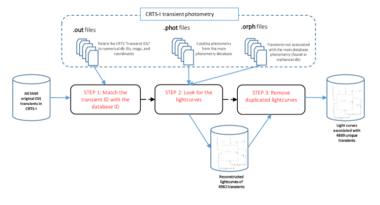
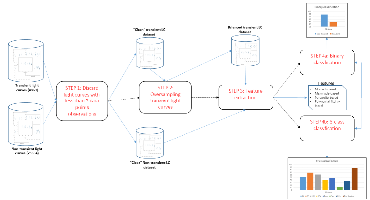
For each one of the 5540 transients reported and classified in the archival webpage http://nesssi.cacr.caltech.edu/catalina/All.arch.html we use its transient IDs and its database IDs to look for the lightcurves in the phot and orphan files. Only 4982 transients can be linked to available data to reconstruct their lightcurves. Furthermore, some of these lightcurves are duplicated, i.e. they had the same number of observations, Modified Julian Date (MJD) and magnitude measurement. We ignore the duplicates to end up with 4869 unique transients with an associated lightcurve. Figure 1 summarizes this process.

Figure 1: MANTRA Dataset Set Up: Lightcurve compilation for transient classes.

The CRTS dataset already provides a classification. The most numerous classes are: supernovae, cataclysmic variable stars, blazars, flares, asteroids, active galactic nuclei, and high-proper-motion stars (HPM). Though most objects in the transient object catalogue belong to a single class, there is some uncertainty in the categorization of some of them. In this case, an interrogation sign is used when a class is not clear e.g. SN? or sometimes multiple possible classes are found for a single event e.g. SN/CV. Table 1 summarizes the number of objects in each class.

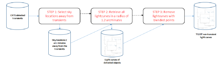
We also compile lightcurves for non-transients. To do that we select sky locations $2$ arcminutes away from the transients. By construction the number of these locations is equal to the number of transients. Then we query http://nesssi.cacr.caltech.edu/cgi-bin/getmulticonedb_release2.cgi to retrieve all lightcurves in a radius of $1.2$ arcminutes. Each point in the retrieved lightcurves has a flag named blend indicating whether the photometry for that source was blended with another source. We only keep the lightcurves that do not have any point labeled as blended. In this way we compile a total number of $71207$ non-transient lightcurves. That is, we have approximately $15$ non-transient for every transient. Figure 2 illustrates this process.

For all lightcurves we compute a reduced $\chi^{2}$ statistic to quantify how different is the lightcurve from a constant lightcurve equal to the its average magnitude

$$\chi^{2}_{r}=\frac{1}{N}\sum_{i=1}^{N}\left(\frac{m_{i}-\bar{m}}{\sigma_{i}}\right)^{2},$$ (1)

where $N$ is the number of points in the lightcurve, $m_{i}$ is the magnitude of the $i$-th data point and $\sigma_{i}$ is its corresponding uncertainty and $\bar{m}$ is the average magnitude over the lightcurve. Not all non-transiet lightcurves have $\chi^{2}_{r}<1$ as one could expect from a statistically flat lightcurve. Either instrumental, atmospheric or intrinsic variability can produce lightcurves with $\chi^{2}_{r}>1$.

In our case we find $25654$ light-curves with $\chi^{2}_{r}<1$ and $45553$ lightcurves with $\chi^{2}_{r}>1$. Lightcurves in the first case are called non-variable and in the latter case variable. In the classification tests we present in this paper we only used non-variable non-transients.

We highlight that we are compiling the classification done by CRTS after they use additional photometric information, spectrometric follow-up, image processing and comparison with other catalogs (Drake et al., 2009; Mahabal et al., 2011) to find a transient. All the possible multiple instrumental and atmospheric effects that might produce variability and $\chi^{2}_{r}>1$ are naturally included in the database and cannot be used a the sole evidence to define a transient. On the same token, not all transients are trivial to detect, some have lightcurves with $\chi^{2}_{r}<1$, usually because they have a small number of measurements close to the faint magnitude limit of the observations.

This means that transient/non-transient classification from lightcurves is a complex task that surely requires more features than simply $\chi^{2}_{r}$. Additional challenges in the classification of lightcurves include the inherent nature of transient events, which is reflected in different brightness behaviors, their evolution over time, and the nonuniform sampling of observations at sequential dates.

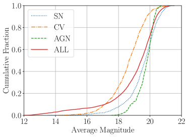
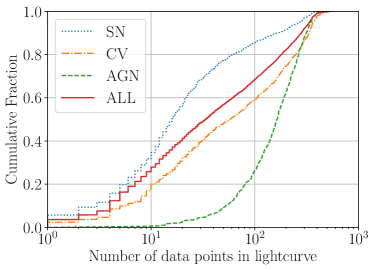
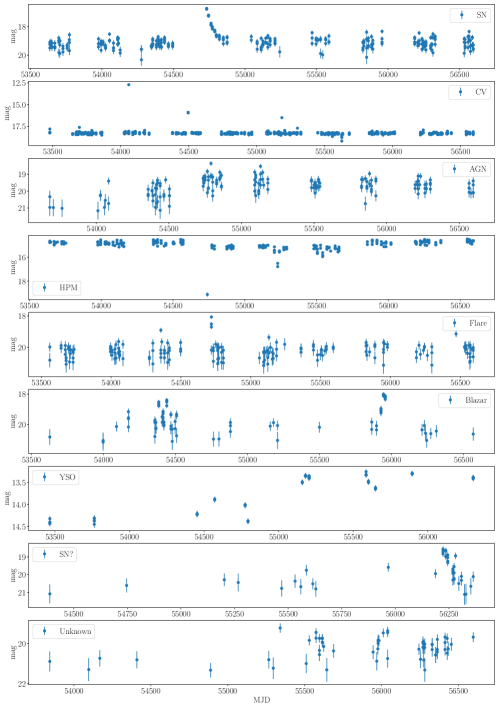
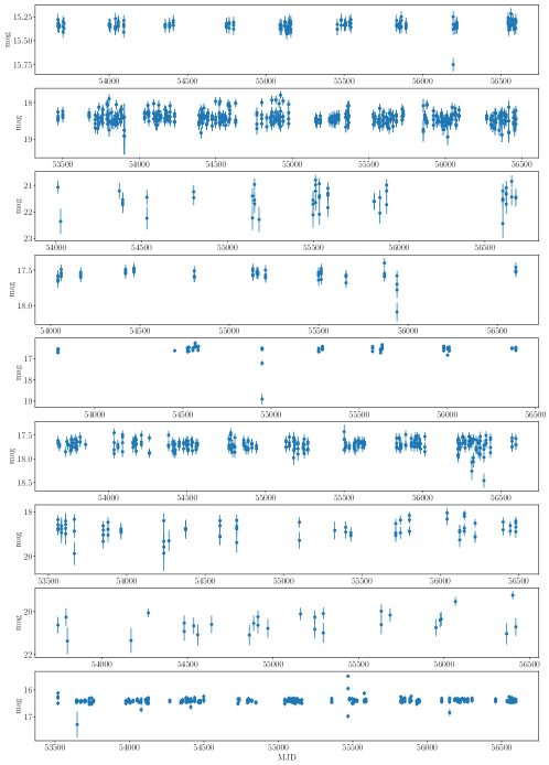
Figure 3 shows the number of lightcurves as a function of average magnitude (left panel) and as a function of the number of points in the lightcurve (right panel). We show separately the whole data set and three most representative classes: supernova, cataclysmic variables and active galactic nuclei. For these four sets, the median magnitude is in the range $18-20$. The number of points in the lightcurve has a larger variability. The median for all the curves is close to 30, while for SN, CV and AGN it is close to 15, 50 and 180, respectively. We provide sample lightcurves of the most represented transient classes and non-transient sources in Figure 4 and Figure 5, respectively. The brightness evolution of non-transient sources is more stable over time, while transient objects present non-periodical changes at different time scales.

Figure 2: MANTRA Dataset Set Up: Lightcurve compilation for non-transients.

Class	Object Count
SN	1723
CV	988
HPM	640
AGN	446
SN?	319
Blazar	243
Unknown	228
Flare	219
AGN?	138
CV?	77

Table 1: Top 10 transient classes in the CRTS with their respective number of lightcurves.

Figure 3: Cumulative number of lightcurves (expressed as a fraction) as a function of average magnitude (left) and number of data points in the lightcurve (right). This includes information for the three most representative classes (SN, CV, AGN) and the whole database (ALL).

Figure 4: Randomly selected lightcurves for the most represented transient classes as compiled in MANTRA. The class of each sample is within the legend box.

Figure 5: Randomly selected lightcurves for non-transient sources retrieved for MANTRA.

2.1 Classification Tasks

We study two classification tasks on the MANTRA dataset:

• Binary Classification. Using a balanced number of events from both classes in order to investigate the capability of distinguishing between transient and non-transient sources.

• 8-Class Classification. Using the unbalanced number of objects across classes to perform a classification into the following categories: AGN, Blazar, CV, Flare, HPM, Other, SN and Non-Transient.

We evaluate both tasks using the metrics of a detection problem. For each class in the testing set, we report the maximum F1-Score that is defined as the harmonic mean of precision and recall. We construct Precision-Recall (PR) curves by setting different thresholds on the output probabilities of belonging to each class.

3 Repository Description

The repository contains the lightcurves and Jupyter notebooks to reproduce some of the Figures and Tables in this paper. The repository can be found in https://github.com/MachineLearningUniandes/MANTRA. To date the repository has two main folders:

• data/lightcurves: contains the transient lightcurves (transient_lightcurves.csv), the labels for the transients (transient_labels.csv), additional information for each transient (transient_info.csv) and the lightcurves for non-transient objects (eight different files nontransient_lightcurves_*.csv). The first two files can be linked by unique transient IDs and provided in the CRTS database.

• nb-explore: includes a Jupyter notebook (explore_light_curves.ipynb) with examples on how to read and plot transient and non-transient lightcurves, extract the statistics in Table 1 and prepare the summary statistics in Figure 3. Additional python files (features.py, helpers.py and inputs.py) allow to read and perform simple operations on the CSV data files.

4 Machine Learning Methods

Here we test baseline algorithms on the MANTRA dataset that can be used as a reference for future work. Figure 6 shows an overview of our transient classification framework. The main steps include and initial data split for non-transients, feature extraction for all lightcurves and classification.

4.1 Split on non-transient variability

Our dataset includes non-transients with different degrees of variability as quantified by the $\chi^{2}_{r}$ statistic defined in Eq. (1). Here we report on the classification experiments using the non-transients with low variability ($\chi^{2}_{r}<1$), that is using 25654 lightcurves out of the total 71207 non-transients in the dataset we are presenting in this paper. These results are presented in great detail in Section 4.5. We perform separately the same classification experiments using only the high variability ($\chi^{2}_{r}\geq 1$) non-transients. Those results are summarized in the Appendix A).

4.2 Preprocessing and Feature Extraction

We do not input directly the annotated lightcurves to the ML algorithms. We perform a preprocessing stage as follows. First, we discard lightcurves with less than 5 data points observations as they may not contain enough information to be classified correctly. The reduction in the dataset is only performed for the purpose of the classification tasks we present in this paper. The public dataset includes all light curves.

Figure 6: Overview of the Machine Learning process on the MANTRA dataset for the binary and 8-class classification tasks. We take the raw lightcurves as input, preprocess the data (step 1) and balance the classes for the training phase (step 2). We extract the features (step 3) that are feed into the ML algorithms that perform the classification task (step 4).

Given that the number of lightcurves per class is imbalanced, in order to have the same number of instances for each class, we implement an oversampling step by artificially generating multiple mock lightcurves from an observed one. We generate a slightly different lightcurve from the observed lightcurve and then sample the observed magnitude from a Gaussian distribution centered on the observational apparent magnitude with the magnitude’s error as the standard deviation. It is important to note that the oversampling was only done on the training set. The test set was left unchanged.

Finally, we compute a standard set of features for each lightcurve. These features are scalars derived from statistical and model-specific fitting techniques. The first features (moment-based, magnitude-based and percentile-based) were formally introduced in Richards et al. (2011), and have been used in other studies (Lochner et al., 2016; D’Isanto et al., 2016). We extend that list to include another set (polynomial fitting-based features) that explicitly take into account the time dependence of the lightcurves.

These groups of features are:

1. Moment-based features, which use the magnitude for each lightcurve.

   • beyond1std: Percentage of observations which are over or under one standard deviation from the weighted average. Each weight is calculated as the inverse of the corresponding observation’s photometric error.

   • kurtosis: The fourth moment of the data distribution.

   • skew: Skewness. Third moment of the data distribution.

   • sk: Small sample kurtosis.

   • std: The standard deviation.

   • stetson_j: The Welch-Stetson J variability index (Stetson, 1996). A robust standard deviation.

   • stetson_k: The Welch-Stetson K variability index (Stetson, 1996). A robust kurtosis measure.

2. Features based on the magnitudes.

   • amp: The difference between the maximum and minimum magnitudes.

   • max_slope: Maximum absolute slope between two consecutive observations.

   • mad: The median of the difference between magnitudes and the median magnitude.

   • mbrp: The percentage of points within 10% of the median magnitude.

   • pst: Percentage of all pairs of consecutive magnitude measurements that have positive slope.

   • pst_last30: Percentage of the last 30 pairs of consecutive magnitudes that have a positive slope, minus percentage of the last 30 pairs of consecutive magnitudes with a negative slope.

   • rcb: Percentage of data points whose magnitude is below 1.5 mag of the median.

   • ls: Period of the peak frequency of the Lomb-Scargle periodogram (Scargle (1982))

3. Percentile-based features, which use the sorted flux distribution for each source. The flux is computed as $F=10^{0.4\mathrm{mag}}$. We define $F_{n,m}$ as the difference between the $m$-th and $n$-the flux percentiles.

   • p_amp: Largest percentage difference between the absolute maximum magnitude and the median.

   • pdfp: Ratio between $F_{5,95}$ and the median flux.

   • fpr20: Ratio $F_{40,60}/F_{5,95}$

   • fpr35: Ratio $F_{32.5,67.5}/F_{5,95}$

   • fpr50: Ratio $F_{25,75}/F_{5,95}$

   • fpr65: Ratio $F_{17.5,82.5}/F_{5,95}$

   • fpr80: Ratio $F_{10,90}/F_{5,95}$

4. Polynomial Fitting-based features, which are the coefficients of multi-level terms in a polynomial curve fitting. This is a new set of features proposed in this paper. Polyn_Tm indicates the coefficient of the term of order m in a fit to a polynomial of order n.

   • Poly1_T1.

   • Poly2_T1.

   • Poly2_T2.

   • Poly3_T1.

   • Poly3_T2.

   • Poly3_T3.

   • Poly4_T1.

   • Poly4_T2.

   • Poly4_T3.

   • Poly4_T4.

4.3 ML algorithms

We conduct experiments with three widely used families of supervised classification algorithms (Bloom et al., 2012; D’Isanto et al., 2016): Neural Networks (NNs), Random Forests (RFs) and Support Vector Machines (SVMs).

These algorithms are popular in published studies and are efficient for low dimensional feature datasets as is our case. We use SciKit-Learn (Pedregosa et al., 2011) Python’s implementation of random forests and support vector machines. Details on the inner workings of these machine learning models can be found in Hastie et al. (2016).

We use the pytorch library for python for the development of the linear Neural Networks. It consists of a series of fully connected layers that map the features to the corresponding number of classes. At each layer, a 1d batch normalization is implemented followed by a rectified linear unit (ReLU) activation function. The final layer calls a softmax activation function to transform the numerical values to class probabilities.

Note that for SVMs, the features were normalized to have zero mean and unit variance. The test set was normalized with respect to the training set. The hyperparameters explored for each algorithm are the following.

• Neural Networks:

  • Learning Rate: $\{0.1,0.01,0.001,0.0001\}$

  • Hidden Layer Sizes: Single , double or triple layers with $500$ nodes each.

• Random Forest:

  • Number of Estimators: $200$ or $700$.

  • Number of features considered: Square root or $log_{2}$ of the total number of features.

• Support Vector Machines:

  • Kernels: Radial Basis Function (RBF), linear or sigmoid.

  • Kernel Coefficient ($\gamma$): $\{0.125,2,32\}$

  • Error Penalty (C): $\{0.125,2,32\}$

4.4 Validation

We split the input lightcurves into training and testing in a $75:25$ ratio respectively, class by class. For the random forests and the SVM, we use a grid search over the hyperparameter combinations with a 2-fold cross-validation over the training set to determine the best hyperparameters. For the neural networks, at each epoch, the network is evaluated on the test data.

4.5 Results

Table 2 shows the average class precision, recall and F1-measure for each of the classification tasks and algorithms listed above.

We also compare our classification with that of D’Isanto et al. (2016). Given that they do not report their F1 scores nor the confusion matrices, we perform the training on our own using their features. The results can be found in Table 4. We find that our results outperform their methodology by $0.87\%$ and $2.87\%$ on the F1 score for the binary and 8-class classification tasks respectively. We consider that modeling the temporal dimension by including the polynomial features is responsible for this improvement. Their relative importance in Figures 9 and 10 supports this hypothesis.

Case	Classifier	Precision	Recall	F1-score
Binary	RF	96.35	96.15	96.25
	SVM	95.33	93.94	94.61
	NN	84.61	84.81	84.71
8 Class	RF	49.12	69.60	52.79
	SVM	33.62	60.34	37.59
	NN	24.14	60.21	29.22

Table 2: Average precision, recall and F1-score accross all classes for each algorithm and classification task. Best results per metric per classification task are in bold.

Figure 7: Confusion Matrix for the best performing model in the Binary task. Rows represent prediction and columns the ground truth.

Figure 8: Confusion Matrix for the best performing model in the 8-class task. The classes follow the abbreviations in Table 3. Rows represent the predictions, and columns the ground truth.

4.5.1 Binary Classification

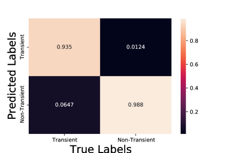
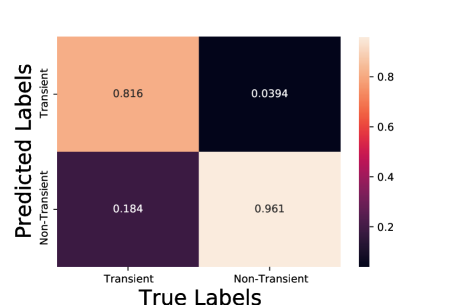
The best algorithm in this task is RFs with an average F1-Score of $96.25\%$. SVMs are the second best-performing model with a F1-Score of $94.61\%$. NNs are ranked third with an F1-Score of $84.71\%$.

Figure 7 shows the confusion matrix of the best performing algorithm. These results suggest that in an imbalanced set up, non-transient sources are better classified while transients are more difficult, showing a difference of about 5 points in the percentage of correct classifications. This difference in performance could be attributed to the intra-class variation within the transients.

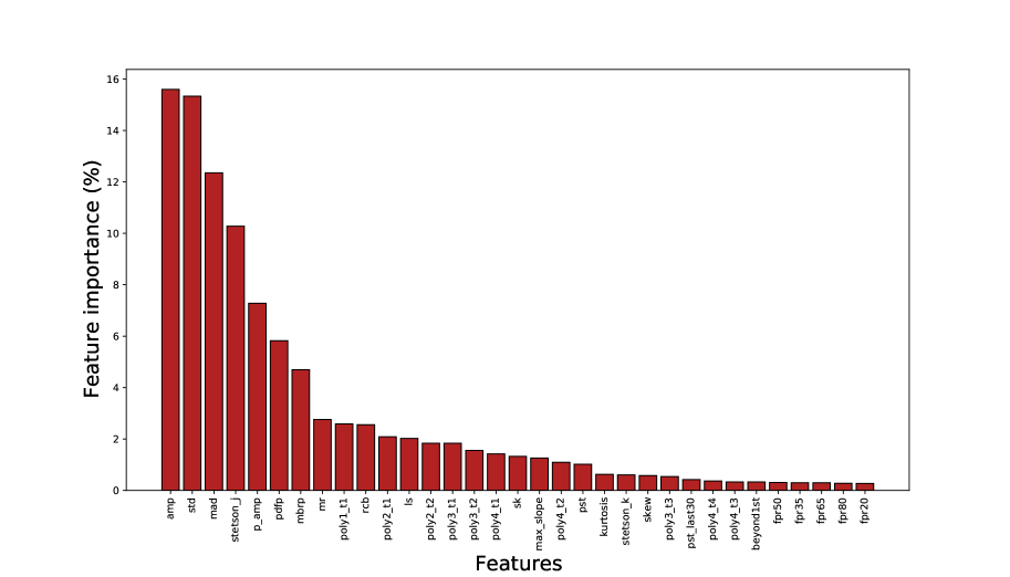
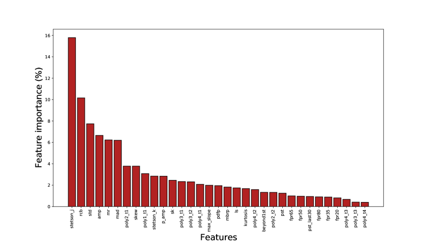
The feature importance list for this problem can be seen in Figure 9. We find that the order of the features is akin to that found by D’Isanto et al. (2016). Their top 5 features ($poly1\_t1$, $std$, $ampl$, $l$ and $skew$) are in our top 10 most important features for classification excluding $ls$ (the lomb-scargle periodogram) which was not included. In general, the first term of the polynomials is significantly more important than the following terms.

Figure 9: Feature importance for the binary classification task.

4.5.2 Eight-Class Classification

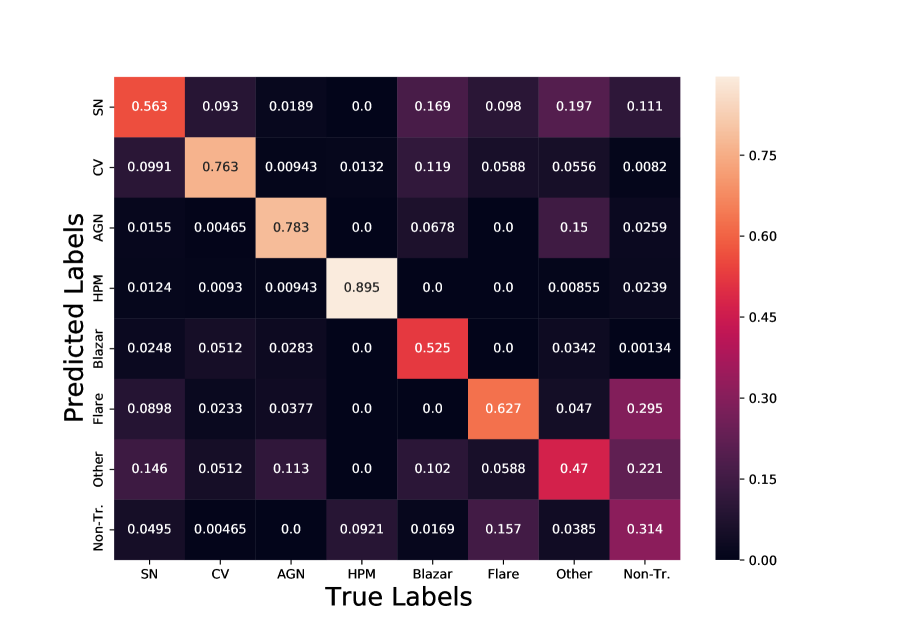
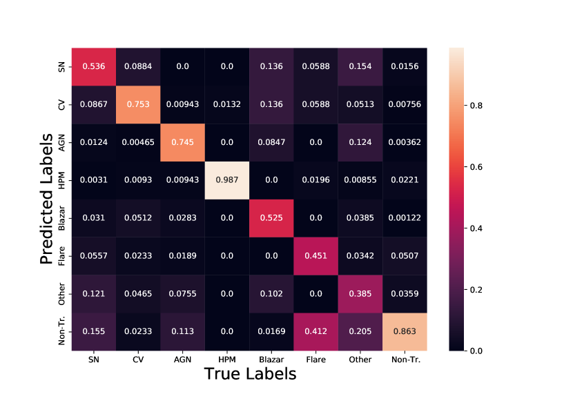
For this task, RF is again the best classifier. The best F1-Score is $52.79\%$. SVMs are the second best model with an F1-Score of $37.59\%$, while NNs are the worst-performing model only achieving an average F1-Score of $29.22\%$. Table 3 summarizes the results for individual classes and Figure 8 presents the confusion matrix for the RF.

The two classes with highest F1-Score are non-transient ($96.83\%$) and CV ($75.23\%$). The recall decreases for the non-transient class in comparison to the binary experiment, meaning that the algorithm misclassified some instances that belong to non-transient class among transient classes. However, transient sources are not commonly confused with non-transient ones. The worst performing classes are Flare, Other and HPM, with F1-Scores in the range 16% - 37%. A possible reason for that is that flaring events are rare and are short lived (lasting tens of minutes) and would then typically span few datapoints in the lightcurve. It is worth noting that the less frequent classes present a lower performance, such as Flare and HPM. Even though the most frequent classes are more easily identified, the "other" type class has a low F1-score due to the diverse nature of sources assigned to this category.

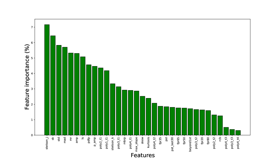
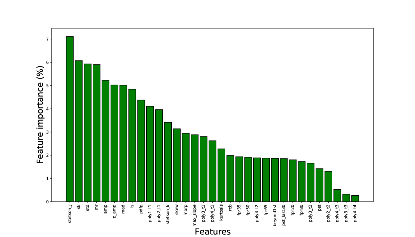
The feature importance list can be found in figure 10. Even though some features have been displaced, the general order with respect to Figure 9 has been preserved.

Class	Precision	Recall	F1-score	Cover
SN	52.91	56.35	54.57	323
CV	74.21	76.28	75.23	215
AGN	63.85	78.30	70.34	106
HPM	9.26	89.47	16.79	76
Blazar	50.82	52.54	51.67	59
Flare	11.99	62.75	20.13	51
Other	30.14	47.01	36.73	234
Non-Tr.	99.76	94.07	96.83	18556
avg/total	49.12	69.60	52.79	19620

Table 3: Precision, Recall and F1-Score for the 8-Class Classification Task.

Figure 10: Feature importance for the 8 class classification task.

Task	Method	Precision	Recall	F1
Binary	D’Isanto	95.92	94.86	95.38
	Ours	96.35	96.15	96.25
8Class	D’Isanto	46.55	66.76	49.92
	Ours	49.12	69.60	52.79

Table 4: Average precision, recall and F1 score for each of the classification tasks. In bold are the best results for each task.

5 Conclusions

The scope of forthcoming large astronomical synoptic surveys motivates the development and exploration of automatized ways to detect transient sources. Such developments require observational datasets to train and test new algorithms. Making these datasets public and easy to access has the potential to open the field to a larger number of contributors. With these goals in mind, in this paper we presented a compilation based on data from the Catalina Real-Time Transient Survey. The dataset has $4869$ transient and $71207$ non-transient lightcurves. The dataset is publicly available at https://github.com/MachineLearningUniandes/MANTRA.

We illustrated how to use this database by extracting characteristic features to use them as input to train three different machine learning algorithms (Random Forests, Neural Networks and Support Vector Machines) for classification tasks. The features extracted from lightcurves were either statistical descriptors of the observations, or polynomial curve fitting coefficients applied to the lightcurves. Overall, the best classifier for all tasks was the Random Forest. Neural Networks showed the worst performance in the binary classification task and the second best in the 8-class classification task.

Certainly other classification algorithms could be used on the MANTRA lightcurves. Our purpose here was not a thorough analysis of machine learning algorithms. Our focus was the compilation of the data into a format that could easily be used for different projects that could be addressed with MANTRA. For instance the supernovae detection problem could be studied as a classification problem between SN and the other classes by using incomplete light curves, mimicking the process of observations that extend the light curve as a survey progresses. Considering extremely unbalanced classes could also be addressed with the dataset we are presenting by simply using less samples for the SN class and keeping a large numbers for the non-transient class.

In a second paper we will present the second part of MANTRA. It corresponds to almost one million images from the CRTS. These will be tested using state-of-the art deep learning techniques for transient classification.

Appendix A Results on the non-transients with high variability

For completeness, we applied the same tasks on the non-transients with high variability ($\chi^{2}_{r}\geq 1$). The main results are in Table 5.

Case	Classifier	Precision	Recall	F1-score
Binary	RF	85.26	88.84	86.93
	NN	84.50	84.44	84.47
	SVM	80.34	82.96	82.79
8 Class	RF	27.50	65.57	33.48
	NN	24.62	59.75	29.49
	SVM	18.86	56.67	21.31

Table 5: Average precision, recall and F1-score across all classes for each algorithm and classification task. Best results per metric per classification task are in bold.

A.1 Binary classification

The best algorithm in the binary task is RFs with an average F1-Score of 86.93%. NN are the second best-performing model with a F1-Score of 84.47%. SVM are ranked third with an F1-Score of 82.79%. The Figure 11 shows the confusion matrix of the best performing algorithm. The Figure 12 shows the feature importance for this problem.

Figure 11: Confusion Matrix for the best performing model in the Binary task. Rows represent prediction and columns the ground truth.

Figure 12: Feature importance for the binary classification task.

A.2 Eight-class classification

The best algorithm in the eight-class task also is RFs with an average F1-Score of 33.48%. SVMs are the second best-performing model with a F1-Score of 21.31%. NNs are ranked third with an F1-Score of 29.49%. The Table 6 summarizes the results for individual classes and the Figure 13 shows the confusion matrix for the best performing algorithm. The Figure 14 shows the feature importance for this problem.

Class	Precision	Recall	F1-score	Cover
SN	19.48	53.56	28.57	323
CV	30.57	75.35	43.49	215
AGN	29.37	74.53	42.13	106
HPM	7.46	98.68	13.88	76
Blazar	26.96	52.54	35.63	59
Flare	1.06	45.10	2.07	51
Other	5.45	38.46	9.55	234
Non-Tr.	99.62	86.33	92.50	41694
avg/total	27.50	65.57	33.48	42758

Table 6: Precision, Recall and F1-Score for the 8-Class Classification Task.

Figure 13: Confusion Matrix for the best performing model in the 8-class task. The classes follow the abbreviations in Table 3. Rows represent the predictions, and columns the ground truth.

Figure 14: Feature importance for the 8 class classification task.

References

- Bellm et al. (2019) Bellm, E. C., Kulkarni, S. R., Graham, M. J., et al. 2019, Publications of the Astronomical Society of the Pacific, 131, 018002, doi: 10.1088/1538-3873/aaecbe
- Bloom et al. (2012) Bloom, J. S., Richards, J. W., Nugent, P. E., et al. 2012, Publications of the Astronomical Society of the Pacific, 124, 1175, doi: 10.1086/668468
- Cabrera-Vives et al. (2017) Cabrera-Vives, G., Reyes, I., Förster, F., Estévez, P. A., & Maureira, J.-C. 2017, ApJ, 836, 97, doi: 10.3847/1538-4357/836/1/97
- D’Isanto et al. (2016) D’Isanto, A., Cavuoti, S., Brescia, M., et al. 2016, MNRAS, 457, 3119, doi: 10.1093/mnras/stw157
- Drake et al. (2009) Drake, A. J., Djorgovski, S. G., Mahabal, A., et al. 2009, ApJ, 696, 870, doi: 10.1088/0004-637X/696/1/870
- Drake et al. (2012) Drake, A. J., Djorgovski, S. G., Mahabal, A., et al. 2012, in IAU Symposium, Vol. 285, New Horizons in Time Domain Astronomy, ed. E. Griffin, R. Hanisch, & R. Seaman, 306–308, doi: 10.1017/S1743921312000889
- Gieseke et al. (2017) Gieseke, F., Bloemen, S., van den Bogaard, C., et al. 2017, MNRAS, 472, 3101, doi: 10.1093/mnras/stx2161
- Hastie et al. (2016) Hastie, T., Tibshirani, R., & Friedman, J. 2016, The Elements of Statistical Learning: Data Mining, Inference, and Prediction, Second Edition (Springer Series in Statistics) (Springer)
- Kaiser (2004) Kaiser, N. 2004, in Society of Photo-Optical Instrumentation Engineers (SPIE) Conference Series, Vol. 5489, Ground-based Telescopes, ed. J. Oschmann, Jacobus M., 11–22, doi: 10.1117/12.552472
- Law et al. (2009) Law, N. M., Kulkarni, S. R., Dekany, R. G., et al. 2009, PASP, 121, 1395, doi: 10.1086/648598
- Lochner et al. (2016) Lochner, M., McEwen, J. D., Peiris, H. V., Lahav, O., & Winter, M. K. 2016, ApJS, 225, 31, doi: 10.3847/0067-0049/225/2/31
- Mahabal et al. (2011) Mahabal, A. A., Djorgovski, S. G., Drake, A. J., et al. 2011, Bulletin of the Astronomical Society of India, 39, 387. https://arxiv.org/abs/1111.0313
- Pedregosa et al. (2011) Pedregosa, F., Varoquaux, G., Gramfort, A., et al. 2011, Journal of machine learning research, 12, 2825
- Richards et al. (2011) Richards, J. W., Starr, D. L., Butler, N. R., et al. 2011, ApJ, 733, 10, doi: 10.1088/0004-637X/733/1/10
- Scargle (1982) Scargle, J. D. 1982, The Astrophysical Journal, 263, 835
- Shappee et al. (2014) Shappee, B. J., Prieto, J. L., Grupe, D., et al. 2014, ApJ, 788, 48, doi: 10.1088/0004-637X/788/1/48
- Stetson (1996) Stetson, P. B. 1996, pasp, 108, 851, doi: 10.1086/133808
- The PLAsTiCC team et al. (2018) The PLAsTiCC team, Allam, Tarek, J., Bahmanyar, A., et al. 2018, arXiv e-prints, arXiv:1810.00001. https://arxiv.org/abs/1810.00001