Discrete correlations of order 2 of generalised
Rudin–Shapiro sequences: a combinatorial approach

Abstract

We introduce a family of block-additive automatic sequences, that are obtained by allocating a weight to each couple of digits, and defining the $n$th term of the sequence as being the total weight of the integer $n$ written in base $k$. Under an additional difference condition on the weight function, these sequences can be interpreted as generalised Rudin–Shapiro sequences, and we prove that they have the same correlations of order $2$ as sequences of symbols chosen uniformly and independently at random. The speed of convergence is very fast and is independent of the prime factor decomposition of $k$. This extends recent work of Tahay [11]. The proof relies on direct observations about base-$k$ representations of integers and combinatorial considerations. We also provide extensions of our results to higher-dimensional block-additive sequences.

Keywords: automatic sequences, pseudorandom sequences, Rudin–Shapiro sequences, difference matrices, discrete correlations

1. 1 Introduction
2. 2 Definitions and presentation of the results
   1. 2.1 Block-additive sequences of rank 2
   2. 2.2 Difference matrices and generalised Rudin–Shapiro sequences
   3. 2.3 Main results
3. 3 Discrete correlations of order 2 of generalised Rudin–Shapiro sequences
   1. 3.1 Frequencies of letters in generalised Rudin–Shapiro sequences
   2. 3.2 Fibre of an integer
   3. 3.3 Proof of Theorem 2.10
   4. 3.4 Correlation matrix
   5. 3.5 Proof of Theorem 2.12
4. 4 Higher dimensional generalised Rudin–Shapiro sequences
5. 5 Extensions and open questions
   1. 5.1 Block-additive sequences of rank larger than 2
   2. 5.2 Can an automatic sequence look even more random?

1 Introduction

A $k$-automatic sequence on a finite set $G$ is a sequence $u\in G^{\mathbb{N}}$ that can be computed by a deterministic finite automaton with output (DFAO) in the following way: the $n$-th term of the sequence is a function of the state reached by the automaton after reading the representation of the integer $n$ in base $k$. Alternatively, a $k$-automatic sequence can also be defined as a sequence generated by a $k$-uniform morphism. We refer to the book of Allouche and Shallit [2] for a complete survey on automatic sequences.

Although automatic sequences are deterministic sequences having a very simple algorithmic description, some of them exhibit a complex behaviour. In this work, we are interested in exploring “how random” an automatic sequence can look like. There are many different ways to measure the “random aspect” of a deterministic sequence. Here, we will study families of automatic sequences having the same discrete correlations of order $2$ as sequences of symbols chosen uniformly and independently at random. We also provide explicit estimates for the speed of convergence.

The sequences we will consider are block-additive sequences. They are obtained by allocating a weight to each couple of digits, and defining the $n$the term of the sequence as being the total weight of the integer $n$ written in base $k$. This weight is obtained by sliding the representation of the integer $n$ in base $k$ with a window of length $2$ (or more generally, of length $\ell\geq 1$), and summing all the weights read. The name block-additive was already used in previous articles [4, 9]. With the terminology of Cateland [3], these sequences are digital sequences. In the special case where the weight matrix is a difference matrix, we will say that the automatic sequence obtained is a generalised Rudin–Shapiro sequence, and prove that it has the same correlations of order $2$ as a sequence of symbols chosen uniformly and independently at random.

As we will comment on further in the article, our terminology of generalised Rudin–Shapiro sequences is consistent with the definitions of [5, 11], and also intersects previous notions of generalised Rudin–Shapiro sequences, such as the one of Quéffelec [10] (see [5] for further references). For other generalisations of the Rudin–Shapiro sequence that we will not investigate here, see Allouche and Shallit [1] and Mauduit and Rivat [8].

As in the articles of Grant et al. [5] and Tahay [11], we study the correlations of order $2$ of generalised Rudin–Shapiro sequences, but rather than making use of exponential sums, we here only employ direct arguments relying on the base-$k$ decomposition of the integers $n$ and $n+r$, for a fixed $r$. This approach highlights the combinatorial role played by the difference condition defining a difference matrix, and allows to obtain more precise estimates on the correlations of order $2$. Furthermore, in addition to studying the asymptotic proportion of integers $n$ satisfying $u_{n}=u_{n+r}$, we provide results on the proportion of integers for which $(u_{n},u_{n+r})=(i,j)$, for any possible value of the couple $(i,j)\in G^{2}$. Precisely, we prove that the limit is equal to $1/|G|^{2}$ for all $(i,j)\in G^{2}$ and for any $r\in{\mathbb{N}}\setminus\{0\}$, as for an i.i.d. sequence of symbols uniformly drawn in $G$. After considering the one-dimensional case, we also mention extensions of our results to higher-dimensional block-additive sequences.

2 Definitions and presentation of the results

In all the article, we denote by $\mathbb{N}$ the set of non-negative integers.

2.1 Block-additive sequences of rank 2

For $k\in{\mathbb{N}}\setminus\{0\}$, we define $\Sigma_{k}=\{0,\ldots,k-1\}$, and we denote by $[n]_{k}$ the representation of the integer $n\in\mathbb{N}$ in base $k$. By definition, it is the unique sequence $x=(x_{i})_{i\in\mathbb{N}}\in\Sigma_{k}^{\mathbb{N}}$ containing finitely many non-zero values, such that

$$n=\sum_{i\in\mathbb{N}}x_{i}k^{i}.$$

We will write

$$\begin{array}[]{rccccc}[n]_{k}=&x_{0}&x_{1}&x_{2}&x_{3}&\cdots\end{array}.$$

We also introduce the notation $\ell_{n}=\min\{i\in\mathbb{N}:\forall j>i,\,x_{i}=0\}$, and we define

$$\sigma_{k}(n)=\sum_{i\in\mathbb{N}}x_{i}=\sum_{i=0}^{\ell_{n}}x_{i},$$

the $k$-ary sum-of-digits function.

Definition 2.1.

Let $(G,+)$ be a finite abelian group, let $k\in{\mathbb{N}}\setminus\{0\}$, and let $f:\Sigma_{k}\times\Sigma_{k}\to G$ be a function satisfying $f(0,0)=0$. We say that the sequence $u=(u_{n})_{n\in\mathbb{N}}\in G^{\mathbb{N}}$ is a block-additive sequence (of rank 2) in base $k$ of weight function (or matrix) $f$ if for any integer $n\in\mathbb{N}$, we have

$$u_{n}=\sum_{i\in\mathbb{N}}f(x_{i},x_{i+1}),$$

where $[n]_{k}=x$.

Example 2.1 (Prouhet–Thue–Morse sequence).

The Prouhet–Thue–Morse sequence is given by

$$\forall n\in\mathbb{N},\quad u_{n}\equiv\sigma_{2}(n)\pmod{2}.$$

The Thue-Morse sequence is a block-additive sequence in base $k=2$, with $G=\mathbb{Z}_{2}$, and weight function $f:\Sigma_{2}\times\Sigma_{2}\to G$ defined by: $\forall(i,j)\in G^{2},f(i,j)=i.$
The first terms are given by $u=(0,1,1,0,1,0,0,1,1,0,0,1,0,1,1,0,\ldots)$.
We represent below a DFAO computing this sequence.

Example 2.2 (Classical Rudin–Shapiro sequence).

The (classical) Rudin–Shapiro sequence on $G=\mathbb{Z}_{2}$ can be defined as the block-additive sequence in base $k=2$ of weight function $f:\Sigma_{2}\times\Sigma_{2}\to G$ given by $\forall(i,j)\in G^{2},\quad f(i,j)=ij$. In other words, $u_{n}$ gives the parity count of the number of (possibly overlapping) occurrences of the block $11$ in the binary expansion of $n$.
The first terms are given by $u=(0,0,0,1,0,0,1,0,0,0,0,1,1,1,0,1,\ldots)$.

The following proposition is straightforward, for the sake of completeness we include the proof.

Proposition 2.3.

If a sequence is block-additive in base $k$, then it is a $k$-automatic sequence.

Proof.

Let $Q=G\times\Sigma_{k}$, $q_{0}=(0,0)$, let $\delta:Q\times\Sigma_{k}\to Q$ be defined by

$$\delta((g,i),j)=(g+f(j,i),j),$$

and let $\tau:Q\to G$ be defined by $\tau(g,i)=g$. The DFAO $(Q,\Sigma_{k},\delta,q_{0},\tau)$ computes the block-additive sequence $u=(u_{n})_{n\in\mathbb{N}}$ of weight function $f$, by reading the representation of the integer $n$ in base $k$ starting with the most significant digit, and using the output map $\tau$. ∎

Remark 2.4.

Alternatively, a block-additive sequence has the following morphic description. Let again $Q=G\times\Sigma_{k}$ and $q_{0}=(0,0)$, and let $\phi:Q^{*}\to Q^{*}$ be the $k$-uniform morphism satisfying, for a state $s=(g,i)\in Q$, $\phi(s)=s_{0}\cdots s_{k-1}$, with $s_{j}=(g+f(j,i),j).$ Consider the fixed point $\phi^{\omega}(q_{0})\in Q^{\mathbb{N}}$. Then, the letter-to-letter projection of $\phi^{\omega}(q_{0})$ by $\tau$ is the block-additive sequence of the function $f$.

Example 2.5.

We represent below the DFAO given by the proof of Prop. 2.3 for the (classical) Rudin–Shapiro sequence.

With the notations $q_{0}=(0,0),q_{1}=(0,1),q_{2}=(1,0),q_{3}=(1,1)$, the $2$-uniform morphism described above is here given by

$$\phi(q_{0})=q_{0}q_{1},\;\phi(q_{1})=q_{0}q_{2},\;\phi(q_{2})=q_{3}q_{1},\;\phi(q_{3})=q_{3}q_{2},$$

with $\tau(q_{0})=\tau(q_{1})=0,\tau(q_{2})=\tau(q_{3})=1.$

2.2 Difference matrices and generalised Rudin–Shapiro sequences

Definition 2.2.

Let $(G,+)$ be a finite abelian group, and let $k\in{\mathbb{N}}\setminus\{0\}$. A difference matrix of size $k$ is a matrix $D=(d(i,j))_{(i,j)\in\Sigma_{k}\times\Sigma_{k}}\in G^{\Sigma_{k}\times\Sigma_{k}}$ satisfying the following difference condition

$$\forall(i,j)\in\Sigma_{k}\times\Sigma_{k}\mbox{ with }\;i\not=j,\quad\forall g\in G,\quad\operatorname*{card}\Big{\{}h\in\Sigma_{k}:d(i,h)-d(j,h)=g\Big{\}}={k\over|G|}.$$

In other words, $D$ is a difference matrix if for any $(i,j)\in\Sigma_{k}\times\Sigma_{k}$ with $i\neq j$, the set $\{d(i,h)-d(j,h):h\in\Sigma_{k}\}$ contains every element of $G$ equally often. Note that the difference condition requires the integer $k$ to be a multiple of $|G|$. We introduce the notation $\pi=k/|G|$, and we have thus $\pi\in{\mathbb{N}}\setminus\{0\}$. We denote by $\mathcal{D}(G,k)$ the set of difference matrices of size $k$ over the group $G$.

Definition 2.3.

A block-additive sequence is a generalised Rudin–Shapiro sequence if its weight function $f$ is such that the matrix $(f(i,j))_{(i,j)\in\Sigma_{k}\times\Sigma_{k}}\in G^{\Sigma_{k}\times\Sigma_{k}}$ is a difference matrix.

Example 2.6.

1. The Thue-Morse sequence is not a generalised Rudin–Shapiro sequence, since its weight function is given by the matrix $\begin{pmatrix}0&0\\ 1&1\end{pmatrix}$, which does not belong to $\mathcal{D}(\mathbb{Z}_{2},2)$.

2. The classical Rudin–Shapiro sequence is a generalised Rudin–Shapiro sequence, since its weight function is given by the matrix $\begin{pmatrix}0&0\\ 0&1\end{pmatrix}$, which belongs to $\mathcal{D}(\mathbb{Z}_{2},2)$.

Let us present different ways to construct difference matrices, and thus to define generalised Rudin–Shapiro sequences.

Example 2.7.

Let $p$ be a prime number, and let $G=\mathbb{Z}_{p}$. Then, the matrix $D=(d(i,j))_{(i,j)\in\Sigma_{p}\times\Sigma_{p}}$ defined by $d(i,j)\equiv ij\pmod{p}$ is a difference matrix. The block-additive sequences thus obtained correspond to Queffélec’s generalisation of the Rudin–Shapiro sequence [10, Section 4]. By definition, if $[n]_{p}=x,$ we have $u_{n}\equiv\sum_{i\in\mathbb{N}}x_{i}x_{i+1}\pmod{p}$.

• As a particular case, for $p=2$, the difference matrix is given by $\begin{pmatrix}0&0\\ 0&1\end{pmatrix}$, and we recover the classical Rudin–Shapiro sequence.

• For $p=3$, the difference matrix is given by $\begin{pmatrix}0&0&0\\ 0&1&2\\ 0&2&1\end{pmatrix}$.

Example 2.8.

For $k=3$, another example of a difference matrix on $G=\mathbb{Z}_{3}$ is given by $\begin{pmatrix}0&1&1\\ 1&0&1\\ 1&1&0\end{pmatrix}$. In the sequence obtained, the term $u_{n}$ counts (modulo 3) the number of blocks of distinct digits in the base-$3$ decomposition of the integer $n$.

It can be seen that for an even integer $k\geq 4$, there exists no difference matrix of size $k$ on $G=\mathbb{Z}_{k}$. Indeed, if $k$ is even, we have $\sum_{i=0}^{k-1}i\equiv{k/2}\pmod{k}$. But if $\sum_{h=0}^{k-1}\left(d(i_{1},h)-d(i_{2},h)\right)\equiv{k/2}\pmod{k}$ and $\sum_{h=0}^{k-1}\left(d(i_{2},h)-d(i_{3},h)\right)\equiv{k/2}\pmod{k}$, then $\sum_{h=0}^{k-1}\left(d(i_{1},h)-d(i_{3},h)\right)\equiv 0\pmod{k}$, so that we obtain a contradiction.

However, the following theorem shows the existence of difference matrices at least for all powers of prime numbers. We include the proof for the sake of clearness.

Theorem 2.9.

[6, Theorem 6.6] For any prime number $p$ and any integers $m,n\in{\mathbb{N}}\setminus\{0\}$ such that $m\leq n$, there exists a finite abelian group $G$ of order $p^{m}$ such that the set $\mathcal{D}(G,p^{n})$ is non-empty.

Proof.

Let $H=\mathbb{F}_{p^{m}}$, and $G=\mathbb{F}_{p^{n}}$ be the finite fields with respectively $p^{m}$ and $p^{n}$ elements. We can represent the elements of $G$ by polynomials of the form $\beta_{0}+\beta_{1}x+\cdots+\beta_{n-1}x^{n-1},$ with $\beta_{0},\ldots,\beta_{n-1}\in\mathbb{Z}_{p}$. The group $(H,+)$ can be seen as the subgroup of $(G,+)$ made of the polynomials of degrees smaller or equal to $m$. Let $\varphi:G\rightarrow H$ be the function which maps the element $\beta_{0}+\beta_{1}x+\cdots+\beta_{n-1}x^{n-1}$ to the element $\beta_{0}+\beta_{1}x+\cdots+\beta_{m-1}x^{m-1}$, and for two polynomials $(\alpha(x),\beta(x))\in G^{2}$, let $d(\alpha(x),\beta(x))=\varphi(\alpha(x)\cdot\beta(x))$, where $\cdot$ denotes the multiplication in the field $G$. Then, one can check that the matrix $D=(d(i,j))_{(i,j)\in\Sigma_{p^{n}}\times\Sigma_{p^{n}}}$ (we identify $\Sigma_{p^{n}}$ with $G$, using any bijection) is a difference matrix on $(G,+)\cong(\mathbb{Z}_{p}^{n},+)$. ∎

Note that there exist difference matrices which do not belong to the families described in the proof of Theorem 2.9 (see [7, p.127] and  [6, Table 6.37]). For example, the matrix

$$\begin{pmatrix}0&0&0&0&0&0\\ 0&0&1&1&2&2\\ 0&1&0&2&1&2\\ 0&1&2&0&2&1\\ 0&2&1&2&0&1\\ 0&2&2&1&1&0\end{pmatrix}$$

is an element of $\mathcal{D}(\mathbb{Z}_{3},6)$ that is not covered by Theorem 2.9.

The enumeration and the classification of difference matrices is a complex task. We refer to [6, 7] for an indepth study of these questions and various examples of difference matrices.

2.3 Main results

We can now state our main results, in the one-dimensional case. We use the notation $\log_{k}(N)$ for the logarithm of $N$ to base $k$.

Theorem 2.10.

If $u$ is a generalised Rudin–Shapiro sequence, then for any $r\in{\mathbb{N}}\setminus\{0\}$, $g\in G$, and $N\in\mathbb{N}$,

$${1\over N}\;\Big{|}\operatorname*{card}\Big{\{}n\in\llbracket 0,N-1\rrbracket:u_{n+r}-u_{n}=g\Big{\}}-{1\over|G|}\Big{|}\,\leq\,r\,k\,{1+\log_{k}(N)\over N}.$$

The limit $1/|G|$ is thus the same as for an i.i.d. sequence of symbols uniformly distributed in $G$. But the convergence is here much faster than in the random case, since the error term is of order $\log(N)/N$, while for i.i.d. sequences, the central limit theorem tells us that it is in $1/\sqrt{N}$.

Remark 2.11.

For $k$ prime or a prime power, the bound in Theorem 2.10 is the same as the one obtained by Tahay [11, Theorem 4]. This is natural since the underlying objects (generalisations of the Rudin–Shapiro sequence) are the same. However, our generalisation of the Rudin–Shapiro sequence to other composed $k$ is different from Tahay [11]: it is directly based on one single difference matrix of size $k$, while Tahay’s construction uses the prime factor decomposition of $k$ and, as a side effect, the error term in his result is $N^{-1/d}$ where $d$ denotes the number of different primes appearing in the prime factor decomposition of $k$ [11, Theorem 5]. The size of our error term for our generalised objects is ${\log(N)}/N$, as $N\rightarrow\infty$, which is much smaller for fixed $r$ and is independent of the arithmetic structure of $k$.

Theorem 2.12.

If $u$ is a generalised Rudin–Shapiro sequence, then for any $r\in{\mathbb{N}}\setminus\{0\}$, and any $(i,j)\in G^{2}$,

$$\lim_{N\to\infty}{1\over N}\;\operatorname*{card}\Big{\{}n\in\llbracket 0,N-1\rrbracket:(u_{n},u_{n+r})=(i,j)\Big{\}}={1\over|G|^{2}}.$$

Remark 2.13.

Tahay obtained several results on the mean value of the discrete correlation coefficients along the integers. The discrete correlation coefficient equals 1 if two symbols are identical, and 0 otherwise [11, Definition 1]. Theorem 2.12 gives a local result that is uniform in the values of the two symbols.

3 Discrete correlations of order 2 of generalised Rudin–Shapiro sequences

The aim of this section is to prove Theorem 2.10 and Theorem 2.12. Namely, we prove that generalised Rudin–Shapiro sequences have the same discrete correlations of order 2 as i.i.d. sequences of symbols, and give a tight estimate of the speed of convergence.

3.1 Frequencies of letters in generalised Rudin–Shapiro sequences

In this section, we present some first general results on generalised Rudin–Shapiro sequences, that we will need afterwards.

Lemma 3.1.

A generalised Rudin–Shapiro sequence is a primitive morphic sequence.

Proof.

As in the proof of Prop. 2.3, let $Q=G\times\Sigma_{k}$, and let $M$ be the matrix indexed by $Q$ and with values in $\{0,1\}$, defined by $M((g,i),(g^{\prime},i^{\prime}))=1$ if and only if there exists $j\in\Sigma_{k}$ such that $(g^{\prime},i^{\prime})=(g+f(j,i),j)$. This matrix thus describes the allowed transitions in the DFAO given in the proof of Prop. 2.3, or equivalently, the incidence matrix of the $k$-uniform morphism defined in Remark 2.4. We prove that all the entries of $M^{2|G|+3}$ are positive (the bound might be not optimal). Let $s_{1}=(g_{1},i_{1})$ and $s_{2}=(g_{2},i_{2})$ be two elements of $Q$. By the difference condition, there exists at least one $h\in G$ such that $f(1,h)-f(0,h)=g_{2}-g_{1}-f(0,1)-f(0,i_{1})-f(i_{2},0).$ From the state $i_{1}$, let us read in the DFAO the sequence $(0,h,0,h,0,h,\ldots,0,h,0,h,1,0,i_{2})$, made of $|G|$ times the pattern $(0,h)$, followed by the pattern $(1,0,i_{2})$. Then, the new state will be $s_{2}$, since

$$f(0,i_{1})+f(h,0)+f(0,h)+f(h,0)+\cdots+f(0,h)+f(h,0)+f(1,h)+f(0,1)+f(i_{2},0)$$

$$=|G|f(h,0)+(|G|-1)f(0,h)+f(1,h)+f(0,1)+f(0,i_{1})+f(i_{2},0)$$

$$=f(1,h)-f(0,h)+f(0,1)+f(0,s_{1})+f(s_{2},0)=g_{2}-g_{1}.$$

The conclusion follows.∎

Proposition 3.2.

If $u$ is a generalised Rudin–Shapiro sequence, then any pattern has a frequency in the sequence $u$. Furthermore, the frequency of each element of $G$ (corresponding to patterns of length 1) is equal to ${1/|G|}$.

Proof.

The existence of the frequencies for all patterns follows from the fact that the sequence $\phi^{\omega}(q_{0})\in Q^{\mathbb{N}}$ is a primitive morphic sequence, where $\phi$ is the morphism given in Remark 2.4. Furthermore, each element of $Q$ has exactly $k$ preimages, since to state $s=(g,j)\in Q$, one can arrive from the state $(g-f(j,i),i)$, for any $i\in G$ (by reading $j$). So, all the elements of $Q$ have the same frequency in $\phi^{\omega}(q_{0})$, and consequently, each element of $G$ has the same frequency in the image of $\phi^{\omega}(q_{0})$ by $\tau$. ∎

3.2 Fibre of an integer

We now introduce the notion of fibre of an integer, that will be useful in our context to study correlations of order $2$ of generalised Rudin–Shapiro sequences.

Let $r\in\mathbb{N}\setminus\{0\}$ be a fixed integer. For $n\in\mathbb{N}$, let us introduce the representations of $n$ and $n+r$ in base $k$ as follows

$$[n]_{k} =x,$$

$$[n+r]_{k} =y.$$

We define the integer

$$c_{n}=\min\{i\in\mathbb{N}:\forall j>i,x_{j}=y_{j}\}.$$

Note that $c_{n}$ depends on $r$, but that for the sake of shortness, we do not mention this dependence in the notation. The integer $c_{n}$ measures how far the carry propagates when adding $r$ to $n$. By definition, $x_{c_{n}}\not=y_{c_{n}}$ and $\forall j>c_{n},$ $x_{j}=y_{j}$. We illustrate the definition of $c_{n}$ below.

$$\begin{array}[]{rccccccc}[n]_{k}=&x_{0}&x_{1}&\cdots&{\color[rgb]{0,0,1}\definecolor[named]{pgfstrokecolor}{rgb}{0,0,1}x_{c_{n}}}&x_{c_{n}+1}&x_{c_{n}+2}&\cdots\\ {[n+r]_{k}}=&y_{0}&y_{1}&\cdots&{\color[rgb]{0,0,1}\definecolor[named]{pgfstrokecolor}{rgb}{0,0,1}y_{c_{n}}}&x_{c_{n}+1}&x_{c_{n}+2}&\cdots\end{array}$$ (1)

We define the fibre of $n$ as the set

$${\mathcal{F}_{r}}(n) =\{m\in\mathbb{N}:x^{\prime}=[m]_{k}\mbox{ satisfies }\forall i\in\mathbb{N}\setminus\{c_{n}+1\},\;x^{\prime}_{i}=x_{i}\}$$

$$=\{n+(\alpha-x_{c_{n}+1})\,k^{c_{n}+1}:\alpha\in\Sigma_{k}\}.$$

We have thus

$$\begin{array}[]{rccccccc}{\mathcal{F}_{r}}(n)=\{\;x_{0}&x_{1}&\cdots&x_{c_{n}}&{\small 0}&x_{c_{n}+2}&x_{c_{n}+3}&\cdots,\\ x_{0}&x_{1}&\cdots&x_{c_{n}}&{\small 1}&x_{c_{n}+2}&x_{c_{n}+3}&\cdots,\\ x_{0}&x_{1}&\cdots&x_{c_{n}}&{\small 2}&x_{c_{n}+2}&x_{c_{n}+3}&\cdots,\\ &&&&\vdots&&&\\ x_{0}&x_{1}&\cdots&x_{c_{n}}&{\small k-1}&x_{c_{n}+2}&x_{c_{n}+3}&\cdots\}.\\ \end{array}$$

Note that if $m\in{\mathcal{F}_{r}}(n)$, then $c_{m}=c_{n}$, so that

$$m\in{\mathcal{F}_{r}}(n)\iff n\in{\mathcal{F}_{r}}(m).$$

Furthermore, let $m\in{\mathcal{F}_{r}}(n)$, and let $x^{\prime}=[m]_{k}$, $y^{\prime}=[m+r]_{k}$. Then, we have

$$y^{\prime}_{c_{n}+1}=x^{\prime}_{c_{n}+1},\quad\mbox{ and }\quad\forall i\in\mathbb{N}\setminus\{c_{n}+1\},\quad y^{\prime}_{i}=y_{i},$$

as represented below:

$$\begin{array}[]{rccccccc}[m]_{k}=\,x^{\prime}=&x_{0}&x_{1}&\cdots&x_{c_{n}}&x^{\prime}_{c_{n}+1}&x_{c_{n}+2}&\cdots\\ {[m+r]_{k}}=\,y^{\prime}=&y_{0}&y_{1}&\cdots&y_{c_{n}}&x^{\prime}_{c_{n}+1}&x_{c_{n}+2}&\cdots\end{array}$$ (2)

Let $u$ be a block-additive sequence in base $k$ of weight $f$, and recall the notation $\pi=k/|G|$. For $n\in\mathbb{N}$, we also introduce the notation $\Delta_{r}(n)=u_{n+r}-u_{n}.$

Proposition 3.3.

If $u$ is a generalised Rudin–Shapiro sequence, then for any $n\in\mathbb{N}$,

$$\forall g\in G,\quad\operatorname*{card}\{m\in{\mathcal{F}_{r}}(n):\Delta_{r}(m)=g\}=\pi.$$

Proof.

By definition of a block-additive sequence, with the notations of (1), we have

$$\Delta_{r}(n) =\sum_{i\in\mathbb{N}}f(y_{i},y_{i+1})-\sum_{i\in\mathbb{N}}f(x_{i},x_{i+1})$$

$$=\sum_{i=0}^{c_{n}}\Big{(}f(y_{i},y_{i+1})-f(x_{i},x_{i+1})\Big{)}.$$

If $m\in{\mathcal{F}_{r}}(n)$, with the notations of (2), we have

$$\Delta_{r}(m)=\sum_{i=0}^{c_{n}}(f(y^{\prime}_{i},y^{\prime}_{i+1})-f(x^{\prime}_{i},x^{\prime}_{i+1})),$$

so that

$$\Delta_{r}(m)-\Delta_{r}(n) =\Big{(}f(y^{\prime}_{c_{n}},y^{\prime}_{c_{n}+1})-f(x^{\prime}_{c_{n}},x^{\prime}_{c_{n}+1})\Big{)}-\Big{(}f(y_{c_{n}},y_{c_{n}+1})-f(x_{c_{n}},x_{c_{n}+1})\Big{)}$$

$$=\Big{(}f(y_{c_{n}},x^{\prime}_{c_{n}+1})-f(x_{c_{n}},x^{\prime}_{c_{n}+1})\Big{)}-\Big{(}f(y_{c_{n}},x_{c_{n}+1})-f(x_{c_{n}},x_{c_{n}+1})\Big{)}$$

It follows that for all $g\in G$,

$$\operatorname*{card}\{m\in{\mathcal{F}_{r}}(n):\Delta_{r}(m)-\Delta_{r}(n)=g\}=\operatorname*{card}\Big{\{}\alpha\in\Sigma_{k}:f(y_{c_{n}},\alpha)-f(x_{c_{n}},\alpha)-A_{n}=g\Big{\}},$$

with $A_{n}=f(y_{c_{n}},x_{c_{n}+1})-f(x_{c_{n}},x_{c_{n}+1}).$

Consequently, if $u$ is a generalised Rudin–Shapiro sequence, then for any $n\in\mathbb{N}$, we have

$$\forall g\in G,\quad\operatorname*{card}\{m\in{\mathcal{F}_{r}}(n):\Delta_{r}(m)-\Delta_{r}(n)=g\}=\pi,$$

and Prop. 3.3 follows. ∎

3.3 Proof of Theorem 2.10

Using the notion of fibre developed above, we obtain the following proposition, from which Theorem 2.10 directly follows, since $\sum_{g\in G}\operatorname*{card}\Big{\{}n\in\llbracket 0,N-1\rrbracket:\Delta_{r}(n)=g\Big{\}}=N$.

Proposition 3.4.

If $u$ is a generalised Rudin–Shapiro sequence, then for any $g\in G$,

$$\operatorname*{card}\Big{\{}n\in\llbracket 0,N-1\rrbracket:\Delta_{r}(n)=g\Big{\}} \geq{\pi N\over k}-\pi\,r\,k-\pi\,r\,\sigma_{k}(N)$$

$$\geq{N\over|G|}-\pi\,r\,k(1+\log_{k}(N)).$$

Proof.

Let $N\in{\mathbb{N}}\setminus\{0\}$, and let $a=[N]_{k}$. We determine the conditions under which an integer $n\in\llbracket 0,N-1\rrbracket$ satisfies ${\mathcal{F}_{r}}(n)\subset\llbracket 0,N-1\rrbracket$. Recall the notation $\ell_{N}=\min\{i\in\mathbb{N}:\forall j>i,a_{i}=0\}$. We can thus write

$$[N]_{k}=a_{0}\;a_{1}\;\cdots\;a_{\ell_{N}-1}\;a_{\ell_{N}}\;0\;0\;\cdots$$

• If $n=a^{\prime}_{\ell_{N}}\,k^{\ell_{N}}+\alpha\,k^{\ell_{N}-1}+\gamma$, for some $\alpha\leq k-1$, $a^{\prime}_{\ell_{N}}<a_{\ell_{N}}$, and $\gamma<k^{\ell_{N}-1}-r$, then $c_{n}\leq\ell_{N}-2$, so that ${\mathcal{F}_{r}}(n)\subset\llbracket 0,N-1\rrbracket$.

  $$[n]_{k} =\underbrace{x_{0}\;x_{1}\;\cdots\;x_{\ell_{N}-2}}_{\gamma<k^{\ell_{N}-1}-r}\;\alpha\;\underbrace{a^{\prime}_{\ell_{N}}}_{<a_{\ell_{N}}}\;0\;0\;\cdots$$

  $$[n+r]_{k} =x^{\prime}_{0}\;x^{\prime}_{1}\;\cdots\;x^{\prime}_{\ell_{N}-2}\;\;\alpha\;\;a^{\prime}_{\ell_{N}}\;\;0\;0\;\cdots$$

• If $n=a_{\ell_{N}}\,k^{\ell_{N}}+a^{\prime}_{\ell_{N}-1}\,k^{\ell_{N}-1}+\alpha\,k^{\ell_{N}-2}+\gamma$, for some $\alpha\leq k-1$, $a^{\prime}_{\ell_{N}-1}<a_{\ell_{N}-1}$, and $\gamma<k^{\ell_{N}-2}-r$, then $c_{n}\leq\ell_{N}-3$, so that ${\mathcal{F}_{r}}(n)\subset\llbracket 0,N-1\rrbracket$.

  $$[n]_{k} =\underbrace{x_{0}\;x_{1}\;\cdots\;x_{\ell_{N}-3}}_{\gamma<k^{\ell_{N}-2}-r}\;\alpha\;\underbrace{a^{\prime}_{\ell_{N}-1}}_{<a_{\ell_{N}-1}}\;a_{\ell_{N}}\;0\;0\;\cdots$$

  $$[n+r]_{k} =x^{\prime}_{0}\;x^{\prime}_{1}\;\cdots\;x^{\prime}_{\ell_{N}-3}\;\;\alpha\;\;a^{\prime}_{\ell_{N}-1}\;\;a_{\ell_{N}}\;0\;0\;\cdots$$

• If $n=a_{\ell_{N}}\,k^{\ell_{N}}+a_{\ell_{N}-1}\,k^{\ell_{N}-1}+a^{\prime}_{\ell_{N}-2}\,k^{\ell_{N}-2}+\alpha\,k^{\ell_{N}-3}+\gamma$, for some $\alpha\leq k-1$, $a^{\prime}_{\ell_{N}-2}<a_{\ell_{N}-2}$, and $\gamma<k^{\ell_{N-3}}-r$, then $c_{n}\leq\ell_{N}-4$, so that ${\mathcal{F}_{r}}(n)\subset\llbracket 0,N\rrbracket$.

  $$[n]_{k} =\underbrace{x_{0}\;x_{1}\;\cdots\;x_{\ell_{N}-4}}_{\gamma<k^{\ell_{N}-3}-r}\;\alpha\;\underbrace{a^{\prime}_{\ell_{N}-2}}_{<a_{\ell_{N}-2}}\;a_{\ell_{N}-1}\;a_{\ell_{N}}\;0\;0\;\cdots$$

  $$[n+r]_{k} =x^{\prime}_{0}\;x^{\prime}_{1}\;\cdots\;x^{\prime}_{\ell_{N}-4}\;\;\alpha\;\;a^{\prime}_{\ell_{N}-2}\;\;a_{\ell_{N}-1}\;a_{\ell_{N}}\;0\;0\;\cdots$$

• And so on, the last condition that will be of interest for us being that if $n=a_{\ell_{N}}\,k^{\ell_{N}}+a_{\ell_{N}-1}\,k^{\ell_{N}-1}+\ldots+a_{\ell_{r}+3}\,k^{\ell_{r}+3}+a^{\prime}_{\ell_{r}+2}\,k^{\ell_{r}+2}+\alpha\,k^{\ell_{r}+1}+\gamma$, for some $\alpha\leq k-1$, $a^{\prime}_{\ell_{r}+2}<a_{\ell_{r}+2}$, and $\gamma<k^{\ell_{r}+1}-r$, then $c_{n}\leq\ell_{r}$, so that ${\mathcal{F}_{r}}(n)\subset\llbracket 0,N-1\rrbracket$.

The number of different integers $n\in\llbracket 0,N-1\rrbracket$ satisfying ${\mathcal{F}_{r}}(n)\subset\llbracket 0,N-1\rrbracket$ that we have exhibited above is equal to

$$\;a_{\ell_{N}}k(k^{\ell_{N}-1}-r)+a_{\ell_{N-1}}k(k^{\ell_{N}-2}-r)+a_{\ell_{N-2}}k(k^{\ell_{N}-3}-r)+\ldots+a_{\ell_{r}+2}k(k^{\ell_{r}+1}-r)$$

$$=\; \;N-(a_{\ell_{r}+1}k^{\ell_{r}+1}+a_{\ell_{r}}k^{\ell_{r}}+\ldots+a_{1}k+a_{0})-r\,k\,(a_{\ell_{N}}+a_{\ell_{N}-1}+a_{\ell_{N}-2}+\ldots+a_{\ell_{r}+2})$$

$$>\; \;N-r\,k^{2}-r\,k\,\sigma_{k}(N).$$

For the last inequality, observe that $a_{\ell_{r}+1}k^{\ell_{r}+1}+a_{\ell_{r}}k^{\ell_{r}}+\ldots+a_{1}k+a_{0}<k^{\ell_{r}+2}\leq r\,k^{2}$. Prop. 3.4 then directly follows from Prop. 3.3. ∎

3.4 Correlation matrix

In order to prove Theorem 2.12, we first introduce the notion of correlation matrix, and formulate the previous results using this terminology.

Let $u\in G^{\mathbb{N}}$ be a fixed sequence. For $r\in{\mathbb{N}}\setminus\{0\},(i,j)\in G^{2}$ and $n\in\mathbb{N}$, we define

$$\delta^{r}_{i,j}(n)=\begin{cases}1&\mbox{ if }(u_{n},u_{n+r})=(i,j),\\ 0&\mbox{ otherwise.}\end{cases}$$

and

$$C^{r}_{i,j}(N)={1\over N}\sum_{n=0}^{N-1}\delta^{r}_{i,j}(n).$$

As a consequence of Prop. 3.2, if $u$ is a generalised Rudin–Shapiro sequence, then for any $r\in{\mathbb{N}}\setminus\{0\}$ and $(i,j)\in G^{2}$, the sequence $C^{r}_{i,j}(N)$ converges when $N$ goes to infinity, so that we can also introduce

$$C^{r}_{i,j}=\lim_{N\to\infty}C^{r}_{i,j}(N).$$

Furthermore, again by Prop. 3.2, for any $i\in G$, the asymptotic frequency of the symbol $i$ is

$$\sum_{j\in G}C^{r}_{i,j}={1\over|G|}.$$

As a consequence of Prop. 3.4, we obtain the following results.

Corollary 3.5.

If $u$ is a generalised Rudin–Shapiro sequence, then for any $(i,j)\in G^{2}$,

$$\sum_{\ell\in G}C^{r}_{i-\ell,j-\ell}(N)\geq{1\over|G|}-\pi\,r\,k{1+\log_{k}(N)\over N}.$$

Corollary 3.6.

If $u$ is a generalised Rudin–Shapiro sequence, then for any $(i,j)\in G^{2}$,

$$\sum_{\ell\in G}C^{r}_{i-\ell,j-\ell}={1\over|G|}.$$

Proof.

It is a consequence from Cor. 3.5 and the observation that $\sum_{(i,j)\in G^{2}}C^{r}_{i,j}=1$. ∎

Note that this result refines the estimates of Tahay concerning the discrete correlation coefficient (cf. Remark 2.13) that detects whether two symbols differ or not. In our language, he proved that

$$\sum_{i\in G}C^{r}_{i,i}={1\over|G|}.$$

3.5 Proof of Theorem 2.12

With the notations above, Theorem 2.12 is equivalent to next proposition, that we now prove. Note that this result is stronger than Corollary 3.6 as it gives the values of the individual terms in the sum.

Proposition 3.7.

If $u$ is a generalised Rudin–Shapiro sequence, then for any $(i,j)\in G^{2}$,

$$C^{r}_{i,j}={1\over|G|^{2}}.$$

Proof.

Let us fix some $\alpha\in\Sigma_{k}$ and consider the integers $n\in\llbracket 0,k^{2N+1}-1\rrbracket$ that are such that the base-$k$ decomposition $x=[n]_{k}$ of $n$ satisfies $x_{N+1}=\alpha$. In other words, $n=m_{1}\,k^{N+1}+\alpha\,k^{N}+m_{2}$, for some integers $m_{1},m_{2}\in\llbracket 0,k^{N}-1\rrbracket$. Assuming furthermore that $m_{2}<k^{N}-r$, we will have $c_{n}<N$, so that

$$(u_{n},u_{n+r})=(u_{km_{1}+\alpha},u_{km_{1}+\alpha})+(u_{\alpha k^{N}+m_{2}},u_{\alpha k^{N}+m_{2}+r}),$$

by definition of a block-additive sequence.

The proof will be based on the following idea: when taking independently at random some integers $m_{1},m_{2}$ uniformly distributed in $\llbracket 0,k^{N}-1\rrbracket$, the distribution of $u_{km_{1}+\alpha}$ converges to the uniform distribution on $G$ when $N$ goes to infinity, while for the second term $(u_{\alpha k^{N}+m_{2}},u_{\alpha k^{N}+m_{2}+r})$, the distribution is asymptotically given by the values $C_{i,j}$ of the correlation matrix. Now, we have $(u_{n},u_{n+r})=(i,j)$ if $u_{km_{1}+\alpha}=\ell$ for some $\ell$ and $(u_{\alpha k^{N}+m_{2}},u_{\alpha k^{N}+m_{2}+r})=(i-\ell,j-\ell)$. Using the independence of $m_{1}$ and $m_{2}$, we thus obtain

$$C^{r}_{i,j}=\sum_{\alpha\in\Sigma_{k}}{1\over k}\sum_{\ell\in G}{1\over|G|}C_{i-\ell,j-\ell}=\sum_{\alpha\in\Sigma_{k}}{1\over k}{1\over|G|}{1\over|G|}={1\over|G|^{2}},$$

since we already know by Corollary 3.6 that for any $(i,j)\in G^{2},\sum_{\ell\in G}C_{i-\ell,j-\ell}={1\over|G|}$.

More formally, let us introduce the following notations, for any $i,j,\ell\in G$,

$$A^{\alpha}_{\ell}(N) =\operatorname*{card}\{m\in\llbracket 0,k^{N}-1\rrbracket:u_{km+\alpha}=\ell\}$$

$$B^{r,\alpha}_{i,j}(N) =\operatorname*{card}\{m\in\llbracket 0,k^{N}-r-1\rrbracket:\delta_{i,j}^{r}(\alpha\,k^{N}+m)=1\}.$$

We claim that for any $\alpha\in\Sigma_{k}$,

$$\lim_{N\to\infty}{A^{\alpha}_{\ell}(N)\over k^{N}}={1\over|G|},\quad\mbox{ and }\quad\lim_{N\to\infty}\sum_{\ell\in G}{B^{r,\alpha}_{i-\ell,j-\ell}(N)\over k^{N}}={1\over|G|}.$$

For the first limit, we use the same tools as for Prop. 3.2. Let $\phi$ be the primitive morphism given in Remark 2.4, so that the sequence $u$ is the image of $\phi^{\omega}(q_{0})$ by $\tau$. One can see that the sequence $(u_{kn+\alpha})_{n\in\mathbb{N}}$ is the image of $\phi^{\omega}(q_{0})$ by the function $\tau^{\prime}:Q\to G$ defined by $\tau^{\prime}(g,i)=g+f(i,\alpha)$. As we have already seen in the proof of Prop. 3.2, all the elements of $Q$ have the same frequency in $\phi^{\omega}(q_{0})$. Consequently, each element of $G$ has the same frequency in the image of $\phi^{\omega}(q_{0})$ by $\tau^{\prime}$. Indeed, for any $g^{\prime}\in G$ and $i\in\Sigma_{k}$, there exists exactly one $g\in G$ such that $\tau^{\prime}(g,i)=g^{\prime}$, so that the cardinal of $\tau^{\prime-1}(\{g^{\prime}\})$ does not depend on the choice of $g^{\prime}$.

The second limit is a small variation of Cor. 3.6, and it can be proven exactly in the same way, using the same steps as in Prop. 3.4. Furthermore, for any $(i,j)\in G^{2}$, we have

$$\sum_{n=0}^{k^{2N+1}-1}\delta_{i,j}^{r}(n)\geq\sum_{\alpha\in\Sigma_{k}}\sum_{\ell\in G}A^{N}_{\ell}(\alpha)\;B^{N}_{i-\ell,j-\ell}(\alpha).$$

It follows that

$$C^{r}_{i,j}(k^{2N+1})\geq{1\over k}\sum_{\alpha\in\Sigma_{k}}\sum_{\ell\in G}{A^{N}_{\ell}(\alpha)\over k^{N}}\;{B^{N}_{i-\ell,j-\ell}(\alpha)\over k^{N}}.$$

When $N$ goes to infinity, we know that the limit of the left term exists and is equal to $C^{r}_{i,j}$. We thus obtain

$$C^{r}_{i,j}\geq{1\over|G|^{2}}.$$

Since $\sum_{(i,j)\in G^{2}}C^{r}_{i,j}=1$, this ends the proof. ∎

4 Higher dimensional generalised Rudin–Shapiro sequences

We propose the following natural extension of Def. 2.1 and 2.3 in dimension $d$. For greater readability, we represent the elements of $\Sigma_{k}^{d}$ as column vectors.

Definition 4.1.

Let $(G,+)$ be a finite abelian group, and let $k\in{\mathbb{N}}\setminus\{0\}$. We say that the sequence $u=(u_{n_{1},\ldots,n_{d}})_{(n_{1},\ldots,n_{d})\in\mathbb{N}^{d}}\in G^{\mathbb{N}^{d}}$ is a $d$-dimensional block-additive sequence in base $k$ if there exists a map $f:\Sigma_{k}^{d}\times\Sigma_{k}^{d}\to G$ satisfying $f\left(\begin{pmatrix}0\\ \vdots\\ 0\end{pmatrix},\begin{pmatrix}0\\ \vdots\\ 0\end{pmatrix}\right)=0$, such that for any integer $n\in\mathbb{N}$, we have

$$u_{n_{1},\ldots,n_{d}}=\sum_{i\in\mathbb{N}}f\left(\begin{pmatrix}x^{1}_{i}\\ \vdots\\ x^{d}_{i}\end{pmatrix},\begin{pmatrix}x^{1}_{i+1}\\ \vdots\\ x^{d}_{i+1}\end{pmatrix}\right)=\sum_{i\in\mathbb{N}}f(x_{i},x_{i+1}),$$

where $x=(x_{i})_{i\in\mathbb{N}}=\begin{pmatrix}x^{1}\\ \vdots\\ x^{d}\end{pmatrix}=\begin{pmatrix}(x_{i}^{1})_{i\in\mathbb{N}}\\ \vdots\\ (x_{i}^{d})_{i\in\mathbb{N}}\end{pmatrix}=\begin{pmatrix}[n_{1}]_{k}\\ \vdots\\ [n_{d}]_{k}\end{pmatrix}$.

We say furthermore that the sequence $u$ is a generalised $d$-dimensional Rudin–Shapiro sequence if the function $f$ satisfies

$$\forall(i,j)\in\Sigma_{k}^{d}\times\Sigma_{k}^{d}\mbox{ with }\;i\not=j,\quad\forall g\in G,\quad\operatorname*{card}\Big{\{}h\in\Sigma_{k}^{d}:f(i,h)-f(j,h)=g\Big{\}}={k\over|G|}.$$

Equivalently, this amounts to saying that the matrix $(f(i,j))_{(i,j)\in\Sigma_{k}^{d}\times\Sigma_{k}^{d}}$ is a difference matrix.

As in the one-dimensional case, a $d$-dimensional sequence that is block-additive in base $k$ is a $k$-automatic sequence.

Let $r\in\mathbb{N}^{d}\setminus\{(0,\ldots,0)\}$. For $n=(n_{1},\ldots,n_{d})\in\mathbb{N}^{d}$, we introduce the representations of $n$ and $n+r$ in base $k$ as follows

$$[n]_{k}=x=\begin{pmatrix}x^{1}\\ \vdots\\ x^{d}\end{pmatrix},\qquad[n+r]_{k}=y=\begin{pmatrix}y^{1}\\ \vdots\\ y^{d}\end{pmatrix},$$

and we define the integer

$$c_{n}=\min\{i\in\mathbb{N}:\;\forall j>i,\,x_{j}=y_{j}\},$$

which measures how far the carry propagates when adding $r$ to $n$.

We define again the fibre of $n$ as the set

$${\mathcal{F}_{r}}(n)=\{m\in\mathbb{N}:x^{\prime}=[m]_{k}\mbox{ satisfies }\forall i\in\mathbb{N}\setminus\{c_{n}+1\},\;x^{\prime}_{i}=x_{i}\},$$

and use the notation $\Delta_{r}(n)=u_{n+r}-u_{n}.$

Since the $d$-dimensional sequence has $d$ components that are all 1-dimensional and independent, the previous arguments can be repeated verbatim.

Proposition 4.1.

If $u$ is a generalised $d$-dimensional Rudin–Shapiro sequence, then for any $n\in\mathbb{N}$,

$$\forall g\in G,\quad\operatorname*{card}\{m\in{\mathcal{F}_{r}}(n):\Delta_{r}(m)=g\}=\pi.$$

We also extend the notations $\delta^{r}$ and $C^{r}$ to $d$-dimensional sequences. Precisely, for $N=(N_{1},\ldots,N_{d})$, we define

$$C^{r}_{i,j}(N)={1\over{N_{1}\cdots N_{d}}}\sum_{\{n\in\mathbb{N}^{d}\,:\,n<N\}}\delta^{r}_{i,j}(n),$$

where we write $n<N$ for $\forall i\in\{1,\ldots,d\},n_{i}<N_{i}$. We also introduce

$$C^{r}_{i,j}=\lim_{N\to\infty}C^{r}_{i,j}(N).$$

Following the previous lines, one can show as in the one-dimensional case that if $u$ is a generalised $d$-dimensional Rudin–Shapiro sequence, then for any $(i,j)\in G^{2}$,

$$\sum_{\ell\in G}C^{r}_{i-\ell,j-\ell}={1\over|G|},$$

which also allows to obtain the following extension of Prop. 3.7.

Proposition 4.2.

If $u$ is a generalised $d$-dimensional Rudin–Shapiro sequence, then for any $(i,j)\in G^{2}$,

$$C^{r}_{i,j}={1\over|G|^{2}}.$$

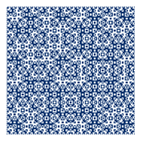
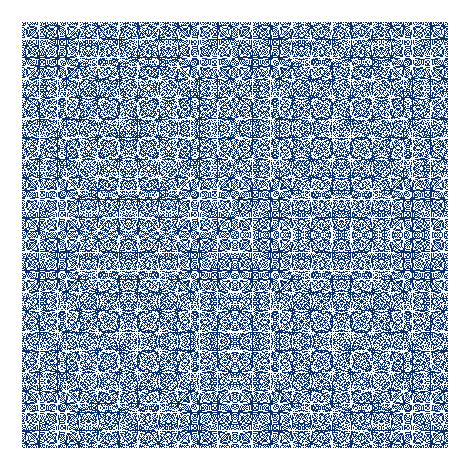
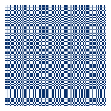
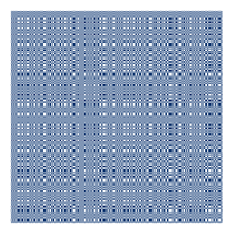
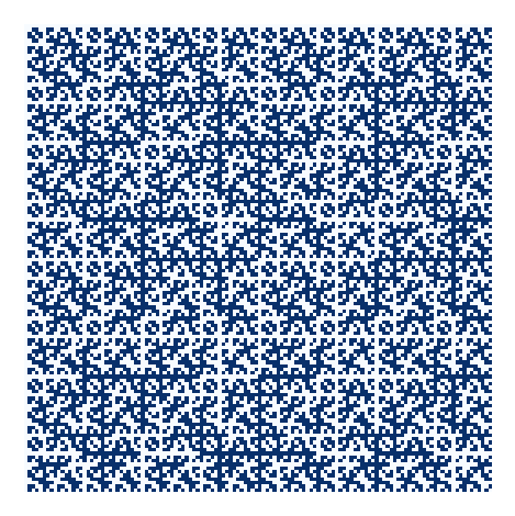
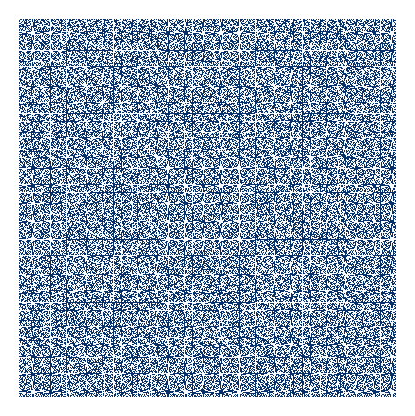
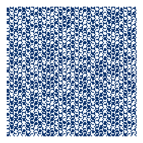
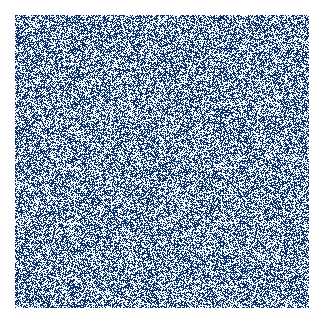
Example 4.3.

We present in Fig. 1 four different examples of generalised Rudin–Shapiro sequence, for $d=2$, $k=2$, $G=\mathbb{Z}_{2}$. For each example, the values of the function $f:\Sigma_{2}^{2}\to\mathbb{Z}_{2}$ is given by a matrix, with the elements of $\Sigma_{2}^{2}$ sorted in the lexicographic order. On the first line of the matrix, one can thus read successively

$$f\left(\begin{pmatrix}0\\ 0\end{pmatrix},\begin{pmatrix}0\\ 0\end{pmatrix}\right),f\left(\begin{pmatrix}0\\ 0\end{pmatrix},\begin{pmatrix}0\\ 1\end{pmatrix}\right),f\left(\begin{pmatrix}0\\ 0\end{pmatrix},\begin{pmatrix}1\\ 0\end{pmatrix}\right),f\left(\begin{pmatrix}0\\ 0\end{pmatrix},\begin{pmatrix}1\\ 1\end{pmatrix}\right),$$

and then on the second line

$$f\left(\begin{pmatrix}0\\ 1\end{pmatrix},\begin{pmatrix}0\\ 0\end{pmatrix}\right),f\left(\begin{pmatrix}0\\ 1\end{pmatrix},\begin{pmatrix}0\\ 1\end{pmatrix}\right),\ldots$$

and so on. On the pictures, the cell $(n_{1},n_{2})\in\mathbb{N}^{2}$ is colored in blue if $u_{n_{1},n_{2}}=1$ and in white if $u_{n_{1},n_{2}}=0$. The corner corresponding to the value $u_{0,0}$ is the bottom-left corner.

Let us present more in detail the first example. For $i,j\in\Sigma_{2}^{2}$, the weight function satisfies $f(i,j)=0$ if $i=j$, and $f(i,j)=1$ otherwise. As an example, we compute below $u_{436,48}$.

$$\begin{array}[]{cccccccccccccl}[436]_{2}&=&0&0&1&0&1&1&0&1&1&0&0&\cdots\\ {[48]_{2}}&=&0&0&0&0&1&1&0&0&0&0&0&\cdots\\ \hline\cr u_{436,48}&\equiv&&0\;+&1\;+&1\;+&1\;+&0\;+&1\;+&1\;+&0\;+&1\;+&0\;+&\cdots\;\equiv 0\pmod{2}\end{array}$$

The following table gives the first values of $u_{n_{1},n_{2}}$, for $(n_{1},n_{2})\in\llbracket 0,2^{3}-1\rrbracket^{2}$.

$$\begin{array}[]{c|ccccccccc}7&1&0&1&0&0&1&0&1\\ 6&0&0&1&1&1&1&0&0\\ 5&1&1&1&1&1&1&1&1\\ 4&0&1&1&0&0&1&1&0\\ 3&1&0&0&1&0&1&1&0\\ 2&0&0&0&0&1&1&1&1\\ 1&1&1&0&0&1&1&0&0\\ 0&0&1&0&1&0&1&0&1\\ \hline\cr{\tiny\;{}^{n_{2}}\diagup\;_{n_{1}}}&0&1&2&3&4&5&6&7\\ \end{array}$$

These values are also contained in the bottom-left $8\times 8$-squares of the two pictures on the first line of Fig. 1.

Concerning the second example, it can be seen that the weight functions satisfies

$$f\left(\begin{pmatrix}i_{1}\\ i_{2}\end{pmatrix},\begin{pmatrix}j_{1}\\ j_{2}\end{pmatrix}\right)\equiv i_{1}j_{1}+i_{2}j_{2}\pmod{2}.$$

As a consequence, the sequence obtained can also be computed by $u_{m,n}=v_{m}+v_{n}$, where $v$ is the classical one-dimensional Rudin–Shapiro sequence.

Matrix	Terms in $\llbracket 0,2^{7}-1\rrbracket^{2}$	Terms in $\llbracket 0,2^{10}-1\rrbracket^{2}$
$\begin{pmatrix}0&1&1&1\\ 1&0&1&1\\ 1&1&0&1\\ 1&1&1&0\end{pmatrix}$
$\begin{pmatrix}0&0&0&0\\ 0&1&0&1\\ 0&0&1&1\\ 0&1&1&0\end{pmatrix}$
$\begin{pmatrix}0&0&0&0\\ 0&0&1&1\\ 0&1&0&1\\ 0&1&1&0\end{pmatrix}$
$\begin{pmatrix}0&0&1&1\\ 0&1&0&1\\ 0&0&0&0\\ 0&1&1&0\end{pmatrix}$

Figure 1: Examples of generalised $2$-dimensional Rudin–Shapiro sequence in base $2$

5 Extensions and open questions

5.1 Block-additive sequences of rank larger than 2

Until now, we have only considered block-additive of rank 2. More generally, we can consider the notion of block-additive function of rank $L$, for an integer $L\in{\mathbb{N}}\setminus\{0\}$, in the sense of Cateland [3].

Definition 5.1.

Let $(G,+)$ be a finite abelian group, let $k\in{\mathbb{N}}\setminus\{0\}$, and let $f:\Sigma_{k}^{L}\to G$ be a function satisfying $f(0,0,\ldots,0)=0$. We say that the sequence $u=(u_{n})_{n\in\mathbb{N}}\in G^{\mathbb{N}}$ is a block-additive sequence (of rank $L$) in base $k$ of weight function $f$ if for any integer $n\in\mathbb{N}$, we have

$$u_{n}=\sum_{i\in\mathbb{N}}f(x_{i},x_{i+1},\ldots,x_{i+L-1}),$$

where $[n]_{k}=x$.

Let $(G,+)$ be a finite abelian group, and let $k\in{\mathbb{N}}\setminus\{0\}$. We say that the function $d:\Sigma_{k}^{L}\to G$ satisfies the difference condition (of rank $L$) if:

$$\forall(i,j)\in\Sigma_{k}\times\Sigma_{k}\mbox{ with }\;i\not=j,\quad\forall(x_{2},\ldots,x_{L-1})\in\Sigma_{k}^{L-2},$$

$$\forall g\in G,\quad\operatorname*{card}\{h\in\Sigma_{k}:d(i,x_{2},\ldots,x_{L-1},h)-d(j,x_{2},\ldots,x_{L-1},h)=g\}={k\over|G|}.$$

The difference condition is a sufficient condition for obtaining the same results as in Section 3.

Example 5.1.

Let us set $k=2$, $G=\mathbb{Z}_{2}$, and let $f:\Sigma_{k}^{3}\to G$ be defined by $f(x,y,z)=\begin{cases}0\mbox{ if }x=y=z\\ 1\mbox{ otherwise.}\end{cases}$. This function satisfies the difference condition. Consequently, the block-additive sequence $u=(u_{n})_{n\in\mathbb{N}}$ of weight function $f$, which is such that $u_{n}$ counts (modulo $2$) the number of blocks different from $000$ and $111$ in the binary representation of $n$, has the same correlations of order $2$ as a binary sequence chosen uniformly at random.

Open question 5.2.

How can we generate functions satisfying the difference condition of rank $L$? Could there be a weaker condition on the weight function for which the block-additive sequences obtained would have the same correlations of order $2$?

5.2 Can an automatic sequence look even more random?

Another possible direction of research consists in trying to construct block-additive sequences for which not only the correlations of order $2$, but also correlations of higher order would be the same as for uniform random sequences. Precisely, for integers $0<r_{1}<\ldots<r_{\ell-1}$, and for a choice $(i_{0},\ldots,i_{\ell-1})\in G^{\ell}$, we introduce

$$\delta^{r}_{i_{0},\ldots,i_{\ell-1}}(n)=\begin{cases}1&\mbox{ if }(u_{n},u_{n+r_{1}},\ldots,u_{n+r_{\ell-1}})=(i_{0},\ldots,i_{\ell-1}),\\ 0&\mbox{ otherwise,}\end{cases}$$

and we look at the asymptotic behaviour of ${1\over N}\sum_{n=0}^{N-1}\delta^{r}_{(i_{0},\ldots,i_{\ell-1})}(n)$, when $N$ goes to infinity. We say that a sequence has the same correlations of order $\ell$ as a uniform random sequence if for any choice of $0<r_{1}<\ldots<r_{\ell-1}$, and for any $(i_{0},\ldots,i_{\ell-1})\in G^{\ell}$,

$$\lim_{N\to\infty}{1\over N}\sum_{n=0}^{N-1}\delta^{r}_{i_{0},\ldots,i_{\ell-1}}(n)={1\over|G|^{\ell}}.$$

Open question 5.3.

For a given $\ell\geq 3$, is it possible to construct a block-additive sequence having the same correlations of order $\ell$ as a uniform random sequence?

Note that it is not possible to construct an automatic sequence such that for any $\ell\geq 1$, the correlations of order $\ell$ would be the same as for a uniform random sequence. Indeed, this would in particular imply the sequence to be normal, while the complexity of an automatic sequence is at most linear.

References

- [1] Jean-Paul Allouche and Jeffrey Shallit. Complexité des suites de Rudin-Shapiro généralisées. J. Théor. Nombres Bordeaux, 5(2):283–302, 1993.
- [2] Jean-Paul Allouche and Jeffrey Shallit. Automatic sequences. Cambridge University Press, Cambridge, 2003. Theory, applications, generalizations.
- [3] Emmanuel Cateland. Digital sequences and k-regular sequences. Theses, Université Sciences et Technologies - Bordeaux I, June 1992.
- [4] Michael Drmota, Peter J. Grabner, and Pierre Liardet. Block additive functions on the Gaussian integers. Acta Arith., 135(4):299–332, 2008.
- [5] Elyot Grant, Jeffrey Shallit, and Thomas Stoll. Bounds for the discrete correlation of infinite sequences on symbols and generalized Rudin-Shapiro sequences. Acta Arith., 140(4):345–368, 2009.
- [6] A. S. Hedayat, N. J. A. Sloane, and John Stufken. Orthogonal arrays. Springer Series in Statistics. Springer-Verlag, New York, 1999. Theory and applications, With a foreword by C. R. Rao.
- [7] P. H. J. Lampio. Classification of difference matrices and complex Hadamard matrices. PhD thesis, Aalto University, 2015.
- [8] Christian Mauduit and Joël Rivat. Prime numbers along Rudin-Shapiro sequences. J. Eur. Math. Soc. (JEMS), 17(10):2595–2642, 2015.
- [9] Clemens Müllner. The Rudin-Shapiro sequence and similar sequences are normal along squares. Canad. J. Math., 70(5):1096–1129, 2018.
- [10] Martine Queffélec. Une nouvelle propriété des suites de Rudin-Shapiro. Ann. Inst. Fourier (Grenoble), 37(2):115–138, 1987.
- [11] Pierre-Adrien Tahay. Discrete correlation of order 2 of generalized Rudin-Shapiro sequences on alphabets of arbitrary size. Unif. Distrib. Theory, 15(1):1–26, 2020.