Clinical Risk Prediction with Temporal Probabilistic
Asymmetric Multi-Task Learning

Abstract

Although recent multi-task learning methods have shown to be effective in improving the generalization of deep neural networks, they should be used with caution for safety-critical applications, such as clinical risk prediction. This is because even if they achieve improved task-average performance, they may still yield degraded performance on individual tasks, which may be critical (e.g., prediction of mortality risk). Existing asymmetric multi-task learning methods tackle this negative transfer problem by performing knowledge transfer from tasks with low loss to tasks with high loss. However, using loss as a measure of reliability is risky since low loss could result from overfitting. In the case of time-series prediction tasks, knowledge learned for one task (e.g., predicting the sepsis onset) at a specific timestep may be useful for learning another task (e.g., prediction of mortality) at a later timestep, but lack of loss at each timestep makes it challenging to measure the reliability at each timestep. To capture such dynamically changing asymmetric relationships between tasks in time-series data, we propose a novel temporal asymmetric multi-task learning model that performs knowledge transfer from certain tasks/timesteps to relevant uncertain tasks, based on the feature-level uncertainty. We validate our model on multiple clinical risk prediction tasks against various deep learning models for time-series prediction, which our model significantly outperforms without any sign of negative transfer. Further qualitative analysis of learned knowledge graphs by clinicians shows that they are helpful in analyzing the predictions of the model.

Introduction

Multi-task learning (MTL) [2] is a method to train a model, or multiple models jointly for multiple tasks to obtain improved generalization, by sharing knowledge among them. One of the most critical problems in multi-task learning is the problem known as negative transfer, where unreliable knowledge from other tasks adversely affects the target task. This negative transfer could be fatal for safety-critical applications such as clinical risk prediction, where we cannot risk losing performance on any of the tasks. To prevent negative transfer, researchers have sought ways to allow knowledge transfer only among closely related tasks, by either identifying the task groups or learning optimal sharing structures among tasks [6, 24]. However, it is not only the task relatedness that matters, but also the relative reliability of the task-specific knowledge. Recent asymmetric multi-task learning (AMTL) models [18, 19] tackle this challenge by allowing tasks with low loss to transfer more.

While the asymmetric knowledge transfer between tasks is useful, it does not fully exploit the asymmetry in time-series analysis, which has an additional dimension of the time axis. With time-series data, knowledge transfer direction may need to be different depending on the timestep. For instance, suppose that we predict an event of infection or mortality within $48$ hours of admission in intensive care units (ICU) based on electronic health records (EHR). At earlier timesteps, prediction of Infection may be more reliable than Mortality, where we may want knowledge transfer to happen from task Infection to Mortality; at later timesteps, we may want the next situation to happen. Moreover, knowledge transfer may happen across timesteps. For example, a high risk of Infection in early timestep will alert high risk of Mortality at later timesteps. To exploit such temporal relationships between tasks, we need a model that does not perform static knowledge transfer between two tasks (Figure 1(a)), but transfers knowledge across the timesteps of two different tasks, while dynamically changing the knowledge transfer amount and direction at each timestep (Figure 1(b)). To this end, we propose a multi-task learning framework for time-series data, where each task not only learns its own latent features at each timestep but also leverages aggregated latent features from the other tasks at the same or different timesteps via attention allocation (Figure 2).

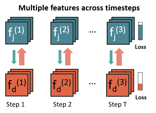
(a) Loss-based AMTL

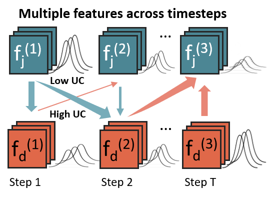
(b) TPAMTL

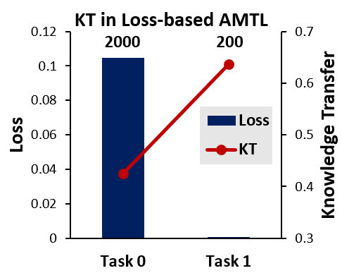
(c)

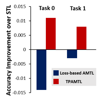
(d)

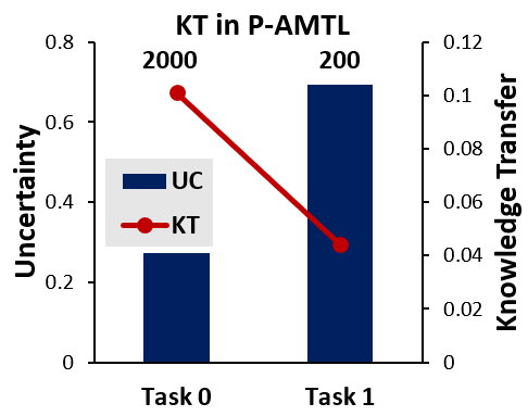
(e)

Figure 1: Concept: (a) Existing AMTL models [18, 19] utilize task loss to perform static knowledge transfer (KT) from one task to another; thus it cannot capture dynamically changing relationships between timesteps and tasks in the time-series domain. (b) Our model performs dynamic KT among tasks and across timesteps based on the feature-level uncertainty (UC). (c-e) Failure case of Loss-based AMTL (Table 1), with a small, imbalanced number of training instances (Task 0: 2000 instances, Task1: 200 instances).

Yet this brings in another challenge. On what basis should we promote asymmetric knowledge transfer? For asymmetric knowledge transfer between tasks, we could use task loss as a proxy of knowledge reliability [18, 19]. However, loss is not a direct measure of reliability, as loss might not be available at every step for time-series prediction. Also, a model trained with few instances (Task 1 in Figure 1(c) - 1(e)) may have a small loss and thus transfer more knowledge to other tasks (Figure 1(c)), but the knowledge from this model could be highly biased and unreliable as it may have overfitted (Figure 1(d)). Thus, we propose a novel probabilistic Bayesian framework for asymmetric knowledge transfer, which leverages feature-level uncertainty, instead of task loss, to measure the reliability of the knowledge (Figure 1(b)). Basically, if a latent feature learned at a certain timestep has large uncertainty, our model will allocate small attention values for the feature; that is, the attention will be attenuated based on the uncertainty, where knowledge transfers from the task with low uncertainty to high uncertainty (Figure 1(e); Please see Table 1).

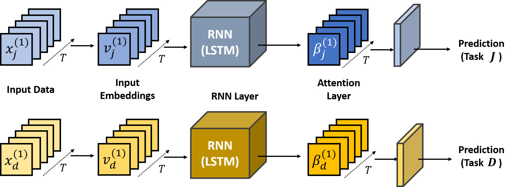
(a) Single Task Learning with LSTM

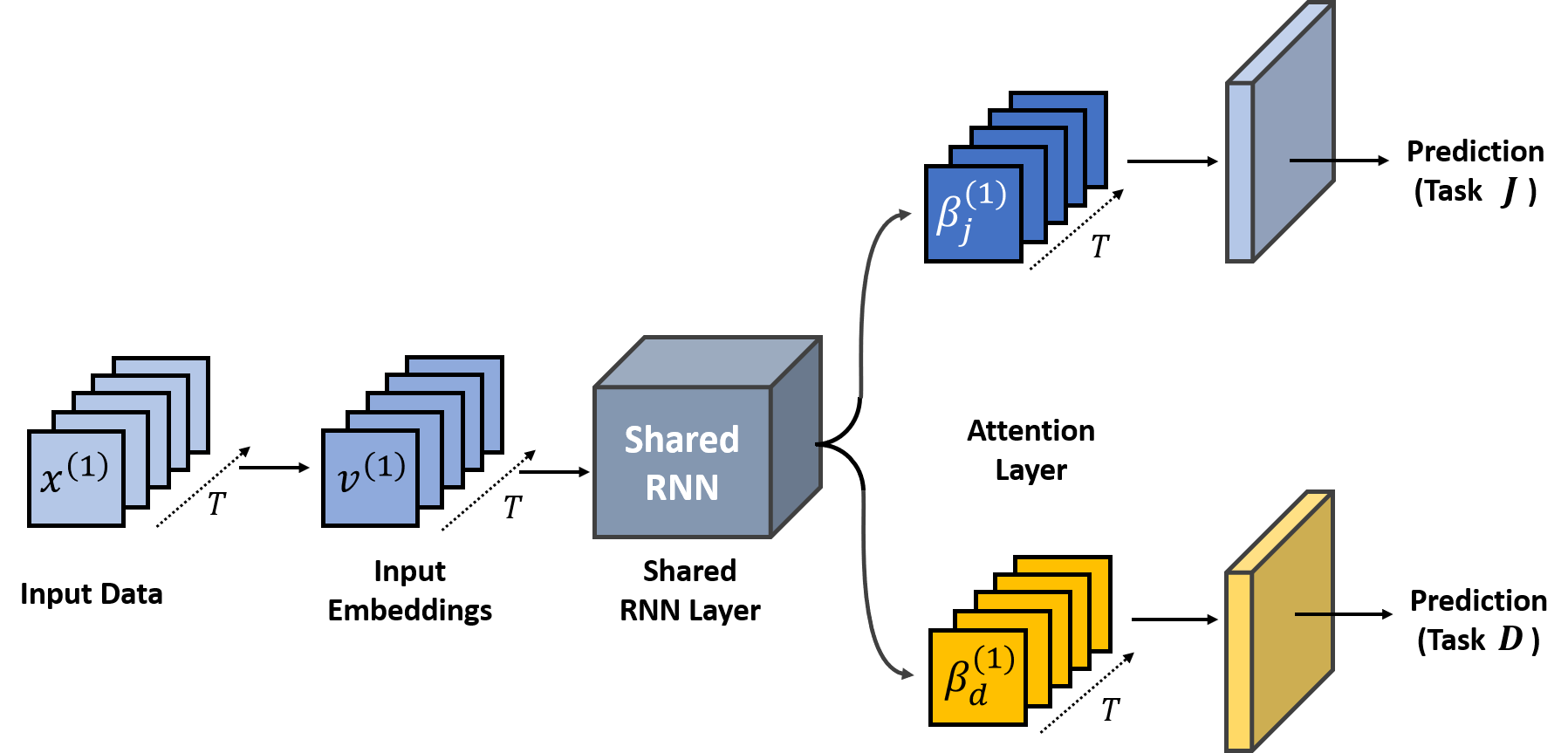
(b) Multi-Task Learning with LSTM

Figure 9: (a) Single- and (b) Multi-Task Learning with LSTM

We experimentally validate our Temporal Probabilistic Asymmetric Multi-Task Learning (TP-AMTL) model on four clinical risk prediction datasets against multiple baselines. The results show that our model obtains significant improvements over strong multi-task learning baselines with no negative transfer on any of the tasks (Table 2). We further show that both the asymmetric knowledge transfer between tasks at two different timesteps and the uncertainty-based attenuation of attention weights are effective in improving generalization. Finally, with the actual knowledge transfer graph plotted with uncertainty obtained for each timestep, we could interpret the model behaviors according to actual clinical events in clinical risk prediction tasks (Figure 3, Supplemenatary Figure 9, 10). This interpretability makes it more suitable for clinical risk prediction in real-world situations.

Our contribution is threefold:

• We propose a novel probabilistic formulation for asymmetric knowledge transfer, where the amount of knowledge transfer depends on the feature level uncertainty.

• We extend the framework to an asymmetric multi-task learning framework for time-series analysis, which utilizes feature-level uncertainty to perform knowledge transfer among tasks and across timesteps, thereby exploiting both the task-relatedness and temporal dependencies.

• We validate our model on four clinical risk prediction tasks against ten baselines, which it significantly outperforms with no negative transfer. With the help of clinicians, we further analyze the learned knowledge transfer graph to discover meaningful relationships between clinical events.

Related Work

Multi-task Learning

While the literature on multi-task learning [2, 1] is vast, we selectively mention the prior works that are closely related to ours. Historically, multi-task learning models have focused on what to share [37, 38, 30], as the jointly learned models could share instances, parameters, or features [13, 16, 22]. With deep learning, multi-task learning can be implemented rather straightforwardly by making multiple tasks to share the same deep network. However, since solving different tasks will require diversified knowledge, complete sharing of the underlying network may be suboptimal and brings in a problem known as negative transfer, where certain tasks are negatively affected by knowledge sharing. To prevent this, researchers are exploring more effective knowledge sharing structures. Soft parameter sharing method with regularizer [6] can enforce the network parameters for each task to be similar, while a method to learn the optimal combination of shared and task-specific representations is also proposed [24] in computer vision. Losses can be weighed based on the uncertainty of the task in a multi-task framework [15], reducing negative transfer from uncertain tasks. While finding a good sharing structure can alleviate negative transfer, negative transfer will persist if we perform symmetric knowledge transfer among tasks. To resolve this symmetry issue, the asymmetric MTL model with inter-task knowledge transfer [18] was proposed, which allows task-specific parameters for tasks with smaller loss to transfer more. Lee, Yang, and Hwang [19] proposed a model for asymmetric task-to-feature transfer that allows reconstructing features with task-specific features while considering their loss, which is more suitable for deep neural networks and scalable.

Clinical time-series analysis

While our method is generic and applicable to any time-series prediction task, we mainly focus on clinical time-series analysis in this paper. Multiple clinical benchmark datasets [5, 12] have been released and publicly available. Also, several recent works have proposed clinical prediction benchmarks with publicly available datasets [3, 9, 11, 26, 27]. We construct our datasets and tasks specific to our problem set (Experiments section), in part referring to previous benchmark tasks. Furthermore, there has been some progress on this topic recently, mostly focusing on the interpretability and reliability of the model. An attention-based model [4] that generates attention for both the timesteps (hospital visits) and features (medical examination results) was proposed to provide interpretations of the predictions. However, attentions are often unreliable since they are learned in a weakly-supervised manner, and a probabilistic attention mechanism [10] was also proposed to obtain reliable interpretation and prediction that considers uncertainty as to how to trust the input. Our work shares the motivation with these prior works as we target interpretability and reliability. Recently, SAnD [31]) proposes to utilize a self-attention architecture for clinical prediction tasks, and Adacare [21] proposes scale-adaptive recalibration module with dilated convolution to capture time-series biomarker features. Yet, they are inherently susceptible to negative transfer as all tasks share a single base network (Table 2).

Approach

Probabilistic Asymmetric Multi-Task Learning

In this section, we describe our framework of probabilistic asymmetric multi-task learning (P-AMTL) in a general setting. Suppose that we have $D$ tasks with datasets $\{\mathbf{X}_{d},\mathbf{Y}_{d}\}_{d=1}^{D}$, in which the sets $\mathbf{X}_{1},\mathbf{X}_{2},...,\mathbf{X}_{D}$ can be identical, overlapping or even disjoint. We further suppose that we have $D$ different probabilistic networks $\{p_{d}(.)\}_{d=1}^{D}$ , each of which generates high-level latent features of task $d$ (task-specific) via $\mathbf{Z}_{d}\sim p_{d}(\mathbf{X}_{d})$. In a single-task learning setting, these latent features $\mathbf{Z}_{d}$ are in turn used to make predictions for task $d$. However, in our asymmetric multi-task learning framework, we want to borrow some learned features from other tasks to share knowledge and to improve generalization performance. Specifically, in order to perform prediction for task $d$, we leverage latent features learned from other tasks, $\mathbf{Z}_{j,d}\sim p_{j}(\mathbf{X}_{d}),\forall j\neq d$. Given the source features $\mathbf{Z}_{j,d}$ and the target features $\mathbf{Z}_{d}$, the model needs to decide on the following:

1) The amount of knowledge to transfer Existing asymmetric multi-task learning models [18, 19] often use task loss to decide on the amount of knowledge transfer, in a way that tasks with low training loss are allowed to transfer more, while tasks with high loss only receive knowledge from other tasks. However, the task loss may not be a proper measure of the knowledge from the task and also unavailable in some cases (Figure 1(c), cases in Introduction). To overcome these limitations, we propose to learn the amount of knowledge transfer based on the feature-level UC. Our model learns the transfer weight from $\mathbf{Z}_{j,d}$ to $\mathbf{Z}_{d}$ by a small network $F_{j,d}$ (Equation 1). This learnable network takes both $\mathbf{Z}_{j,d}$, $\mathbf{Z}_{d}$ and their variance $\bm{\sigma}^{2}_{j,d}$ and $\bm{\sigma}^{2}_{d}$ as its input. Note that if the variance is not available from the output of $\{p_{d}(.)\}_{d=1}^{D}$ directly, we can perform Monte-Carlo sampling $k$ times on $\mathbf{Z}_{j,d}$ and $\mathbf{Z}_{d}$ to compute the estimates of variances. In practice, we can implement each $F_{j,d}$ as a multi-layer perceptron with the input as the concatenation of $\mathbf{Z}_{j,d},\mathbf{Z}_{d},\bm{\sigma}^{2}_{j,d}\text{ and }\bm{\sigma}^{2}_{d}$.

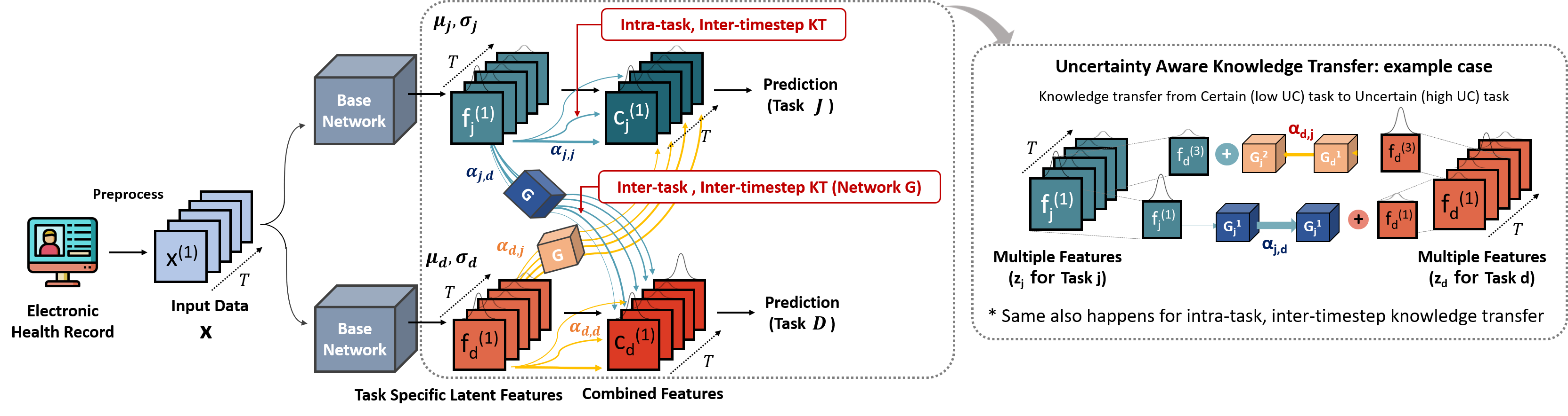
Figure 2: Temporal probabilistic asymmetric knowledge transfer. This figure illustrates how we apply the probabilistic asymmetric knowledge transfer between tasks at the same timestep and across different timesteps. (Right) Features of task $j$ at timestep $1$ is more reliable than features of task $d$ at timestep $1$, so the model will learn to transfer more from task $j$ to task $d$ and transfer less from task $d$ to task $j$.

$$\alpha_{j,d}=F_{j,d}(\mathbf{Z}_{j,d},\mathbf{Z}_{d},\bm{\sigma}^{2}_{j,d},\bm{\sigma}^{2}_{d})$$ (1)

2) The form of transferred knowledge Since the learned features for different tasks may have completely different representations, directly adding $\alpha_{j,d}\mathbf{Z}_{j,d}$ to $\mathbf{Z}_{d}$ would be sub-optimal. For this combining process, we train two additional networks $G^{1}_{k}$ and $G^{2}_{k}$ for each task $k$ where $G^{1}_{k}$ is used to convert the learned task-specific features from $p_{k}(.)$ to a shared latent space and $G^{2}_{k}$ is used to convert the features from that shared latent space back to the task-specific latent space. Finally, we compute the combined feature map for task $d$ as (Figure 2 (Right)):

$$\mathbf{C}_{d}=\mathbf{Z}_{d}+G^{2}_{d}\left(\sum_{j\neq d}\alpha_{j,d}*G^{1}_{j}(\mathbf{Z}_{j,d})\right)$$ (2)

The combined feature map $\mathbf{C}_{d}$ can then be used for the final prediction for task $d$. The combined feature maps for all other tasks are computed in the same manner.

Temporal Probabilistic Asymmetric Multi-Task Learning

We now apply our probabilistic asymmetric multi-task learning framework for the task of time-series prediction.

Our goal is to jointly train time-series prediction models for multiple tasks at once. Suppose that we are given training data for $D$ tasks, $\mathbbm{D}=\{(\mathbf{X}_{1},\mathbf{Y}_{1}),\dots,(\mathbf{X}_{D},\mathbf{Y}_{D})\}$. Further suppose that each data instance $\mathbf{x}\text{ where }\mathbf{x}\in\mathbf{X}_{d}$ for some task $d$, consists of $T$ timesteps. That is, $\mathbf{x}=(\mathbf{x}^{(1)},\mathbf{x}^{(2)},\dots,\mathbf{x}^{(T)})$, where $\mathbf{x}^{(t)}\in\mathbb{R}^{m}$ denotes the data instance for the timestep $t$. Here we assume the number of timesteps $T$ is identical across all tasks for simplicity, but there is no such restriction in our model. Additionally, $y_{d}$ is the label for task $d$; $y_{d}\in\{0,1\}$ for binary classification tasks, and $y_{d}\in\mathbb{R}$ for regression tasks. Given time-series data and tasks, we want to learn the task-specific latent features for each task and timestep, and then perform asymmetric knowledge transfer between them. Our framework is comprised of the following components:

Shared Low-Level Layers

We allow our model to share low-level layers for all tasks in order to learn a common data representation before learning task-specific features. At the lowest layer, we have a shared linear data embedding layer to embed the data instance for each timestep into a continuous shared feature space. Given a time-series data instance $\mathbf{x}$, we first linearly transform the data point for each timestep $t$, $\mathbf{x}^{(t)}\in\mathbbm{R}^{m}$, which contains $m$ variables:

$$(\mathbf{v}^{(1)},\mathbf{v}^{(2)},...,\mathbf{v}^{(T)})=\mathbf{v}=\mathbf{x}\mathbf{W}_{emb}\in\mathbbm{R}^{T\times k}$$ (3)

where $\mathbf{W}_{emb}\in\mathbbm{R}^{m\times k}$ and $k$ is the hidden dimension. This embedded input is then fed into shared RNN layer for pre-processing:

$$\mathbf{r}=(\mathbf{r}^{(1)},\mathbf{r}^{(2)},...,\mathbf{r}^{(T)})=RNN(\mathbf{v}^{(1)},\mathbf{v}^{(2)},...,\mathbf{v}^{(T)})$$ (4)

Task- and Timestep Embedding Layers (‘Base Network’ in Figure 2)

After embedding and pre-processing the input into a continuous space, we further encode them into task- and timestep-specific features. Since hard-sharing layers may result in negative transfer between tasks, we allow separate embedding layers for each task to encode task-specific knowledge in our ‘Base Network’. For each task $d$, the separate network consists of $L$ feed-forward layers, which learn disentangled knowledge for each timestep. These $L$ feed-forward layers for task embedding can be formulated as:

$$\mathbf{h}_{d}=\sigma((...\sigma(\sigma(\mathbf{r}\mathbf{W}^{1}_{d}+\mathbf{b}^{1}_{d})\mathbf{W}^{2}_{d}+\mathbf{b}^{2}_{d})...)\mathbf{W}^{L}_{d}+\mathbf{b}^{L}_{d})\in\mathbbm{R}^{T\times k}$$ (5)

where $\mathbf{W}_{d}^{i}\in\mathbbm{R}^{k\times k},\mathbf{b}_{d}^{i}\in\mathbbm{R}^{k}$ and $\sigma$ is a non-linear activation function (e.g. leaky relu).

Modeling feature-level uncertainty

While the embedding above can capture knowledge for each task and timestep, we want to further model their uncertainties as well, to measure the reliability of the knowledge captured. Towards this objective, we model the latent variables as probabilistic random variables, with two types of UC [14]: 1) epistemic uncertainty, which comes from the model’s unreliability from the lack of training data, and 2) aleatoric uncertainty, that comes from the inherent ambiguity in the data. We capture the former by using dropout variational inference [7], and the latter by explicitly learning the model variance as a function of the input (Figure 2). Suppose that we have the task-specific latent features: $\mathbf{z}_{d}\sim p(\mathbf{z}_{d}|\mathbf{x},\bm{\omega})\text{ where }\bm{\omega}$ is the set of all parameters. This can be formulated as below:

$$\mathbf{z}_{d}|\mathbf{x},\bm{\omega}\sim\mathcal{N}\left(\mathbf{z}_{d};\bm{\mu}_{d},diag(\bm{\sigma}^{2}_{d})\right)$$ (6)

$$\bm{\mu}_{d}=\sigma(\mathbf{h}_{d}\mathbf{W}_{d}^{\mu}+\mathbf{b}_{d}^{\mu})$$ (7)

$$\bm{\sigma}_{d}=softplus(\mathbf{h}_{d}\mathbf{W}_{d}^{\sigma}+\mathbf{b}_{d}^{\sigma})$$ (8)

As mentioned before, we use dropout approximation [7] with parameter $M$ as the variational distribution $q_{M}(\bm{\omega})$ to approximate $p(\bm{\omega}|\mathbbm{D})$.

Asymmetric knowledge transfer across tasks and time steps

Now we apply the proposed probabilistic asymmetric knowledge transfer method to perform knowledge transfer across timesteps, both within each task and across tasks, to exploit intra- and inter-task temporal dependencies. In order to transfer knowledge from task $j$ to task $d$ with temporal dependencies, we allow the latent features of task $d$ at time step $t$ ($\mathbf{f}_{d}^{(t)}$, with $\mathbf{z}_{d}=(\mathbf{f}_{d}^{(1)},\mathbf{f}_{d}^{(2)},...,\mathbf{f}_{d}^{(T)})$) to obtain knowledge from task $j$ at all previous time steps (Figure 2), and then combine them into a single feature map $\mathbf{C}_{d}^{(1)},\mathbf{C}_{d}^{(2)},...,\mathbf{C}_{d}^{(T)}$:

$$\mathbf{C}_{d}^{(t)}=\mathbf{f}_{d}^{(t)}+G^{2}_{d}\left({\sum}^{D}_{j=1}{\sum}_{i=1}^{t}\alpha^{(i,t)}_{j,d}*G^{1}_{j}\left(\mathbf{f}_{j}^{(i)}\right)\right)\forall t$$ (9)

As mentioned in the previous subsection, the transfer weight $\alpha^{(i,t)}_{j,d}$ is computed by a network $F_{j,d}$ with input $\mathbf{f}_{d}^{(t)}$, $\mathbf{f}_{j}^{(i)}$ and their variance $\bm{\sigma}_{d}^{(t)}$, $\bm{\sigma}_{j}^{(i)}$ (again, we perform MC sampling to get the variance).

Here, we choose to constrain the knowledge transfer to happen only from past to future timesteps because of the time complexity at inference time. With our proposed model, for each update at the clinical environment in an online manner, we only need to transfer the knowledge from previous time steps to the current one, making the complexity to be $\mathbf{O(T)}$. This is on a par with other models like RETAIN [4] or UA [10], making it highly scalable (Table 1 of Supplementary File). However, if we allow the knowledge to transfer from future timestep to past timestep, we also need to update the knowledge at previous timesteps for a single update. The time complexity of the model in this case is $O(T^{2})$, which is undesirable. In the ablation study, we show that this constraint also brings in a small performance gain. The total complexity of the whole training or inference is still $O(T^{2})$ due to the inter-timestep transfer, but this is on par with state-of-the-art models such as Transformer [33] and SAnD [31].

Finally, we use the combined features $\mathbf{C}_{d}^{(1)},\mathbf{C}_{d}^{(2)}$,…,$\mathbf{C}_{d}^{(T)}$, which contain temporal dependencies among tasks, for prediction for each task $d$. We use an attention mechanism

$$\bm{\beta}_{d}^{(t)}=tanh\left(\mathbf{C}_{d}^{(t)}\mathbf{W}_{d}^{\beta}+\mathbf{b}_{d}^{\beta}\right)\quad\forall t\in\{1,2,...,T\}$$ (10)

where $\mathbf{W}_{d}^{\beta}\in\mathbbm{R}^{k\times k}$ and $\mathbf{b}_{d}^{\beta}\in\mathbbm{R}^{k}$. Then the model can perform prediction as

$$p_{d}=p(\widehat{y_{d}}|\mathbf{x})=Sigmoid\left(\frac{1}{T}\left({\sum}^{T}_{t=1}\bm{\beta}_{d}^{(t)}\odot\mathbf{v}^{(t)}\right)\mathbf{W}_{d}^{o}+b_{d}^{o}\right)$$ (11)

for classification tasks, where $\odot$ denotes the element-wise multiplication between attention ${\beta_{d}}^{(t)}$ and shared input embedding $\mathbf{v}^{(t)}$ (from Eq. 3), $\mathbf{W}_{d}^{o}\in\mathbbm{R}^{k\times 1}$ and $b_{d}^{o}\in\mathbbm{R}^{1}$. Predictions for other tasks are done similarly. Note that our model does not require each instance to have the labels for every tasks. We can simply maximize the likelihood $p(y_{d}|\mathbf{x})$ whenever the label $y_{d}$ is available for input $x$ for task $d$. Furthermore, our model does not require the instances to have the same number of timesteps $T$.

The loss function of our objective function is:

$$\sum_{x,y} \left[-\sum_{d\in Ta(x)}(y_{d}\log p_{d}+(1-y_{d})\log(1-p_{d}))\right]+\beta_{w\_decay}||\theta||_{2}^{2}$$ (12)

where $Ta(x)$ is the set of tasks which we have the labels available for data instance $x$, $\beta_{w\_decay}$ is the coefficient for weight decay and $\theta$ is the whole parameters of our model.

Experiments

Probabilistic Asymmetric Multi-task Learning

We first validate the effectiveness of the uncertainty-based knowledge transfer for asymmetric multi-task learning, using a non-temporal version of our model. We use a variant [32] of the MNIST dataset [17] which contains images of handwritten digits $0$-$9$ with random rotations and background noise. From this dataset, we construct $5$ tasks; each task is a binary classification of determining whether the given image belongs to class $0$-$4$. We sample 5000, 5000, 1000, 1000, and 500 examples for task 0, 1, 2, 3, and 4 respectively, such that asymmetric knowledge transfer becomes essential to obtain good performance on all tasks. As for the base network, we use a multi-layer perceptron, which outputs mean and variance of the task-specific latent features.
1) Single Task Learning (STL) learns an independent model for each task.
2) Multi Task Learning (MTL) learns a single base network with $5$ disjoint output layers for the $5$ tasks.
3) AMTL-Loss. A model that is similar to P-AMTL, with the transfer weight from task $j$ to task $d$ learned by a network $F_{j,d}$ with the average task loss over all instances as the input.
4) P-AMTL. Our probabilistic asymmetric MTL model.

Results (Table 1) show that MTL outperforms STL, but suffers from negative transfer (Task 4, highlighted in red (Table 1)). AMTL-Loss underperforms MTL, which shows that the loss is not a good measure of reliability; a model that is overfitted to a task will have a small loss, but its knowledge may be unreliable (Figure1(c)). Finally, our model outperforms all baselines without any sign of negative transfer, demonstrating the superiority of uncertainty-based knowledge transfer.

Table 1: AUROC for the MNIST-Variation Experiment

Models	Task 0	Task 1	Task 2	Task 3	Task 4	Average
STL	0.7513$\pm$0.02	0.7253$\pm$0.01	0.5401$\pm$0.01	0.5352$\pm$0.02	0.6639$\pm$0.01	0.6432$\pm$0.01
MTL	0.8266$\pm$0.01	0.7021$\pm$0.01	0.5352$\pm$0.01	0.5987$\pm$0.01	0.6203$\pm$0.02	0.6565$\pm$0.01
AMTL-Loss	0.7317$\pm$0.02	0.7236$\pm$0.01	0.5309$\pm$0.01	0.5166$\pm$0.02	0.6698$\pm$0.01	0.6345$\pm$0.01
P-AMTL (ours)	0.8469$\pm$0.01	0.7267$\pm$0.01	0.5382$\pm$0.01	0.5950$\pm$0.01	0.6822$\pm$0.01	0.6778$\pm$0.01

Clinical risk prediction from EHR

Clinical risks can be defined in various ways, but in this paper, we define clinical risks as the existence of the event (e.g., Heart Failure, Respiratory Failure, Infection, Mortality) that may lead to deterioration of patients’ health condition within a given time window (e.g., $48$ hour).

Tasks and Datasets

We experiment on four datasets where we compile for clinical risk prediction from two open-source EHR datasets. Every dataset used in this paper contain tasks with clear temporal dependencies between them. The input features have been pre-selected by the clinicians, since the excessive features were not clinically meaningful, and may harm the prediction performance. Missing feature values are imputed with zero values. Pleare refer to the supplementary file for the explanation and evaluation on two datasets MIMIC III - Heart Failure and Respiratory Failure.

1) MIMIC III - Infection. We compile a dataset out of the MIMIC III dataset [12], which contains records of patients admitted to ICU of a hospital. We use records of patients over the age $15$, where we hourly sample to construct $48$ timesteps from the first $48$ hours of admission. Following clinician’s guidelines, we select $12$ infection-related variables for the features at each timestep (See Table 8, 9 of supplementary file). Tasks considered for this dataset are the clinical events before and after infection; Fever (Task 1) as the sign of infection with elevated body temperature, Infection (Task 2) as the confirmation of infection by the result of microbiology tests, and finally, Mortality (Task 3) as a possible outcome of infection (See Figure 1 of supplementary file for the task configuration). After pre-processing, approximately $2000$ data points with a sufficient amount of features were selected, which was randomly split to approximately $1000/500/500$ for training/validation/test.

2) PhysioNet [5]. Total of $4,000$ ICU admission records were included, each containing 48 hours of records (sampled hourly) and $31$ physiological signs including variables displayed in Table 3. We select $29$ infection-related variables for the features available at each timestep (See supplementary file). Task used in the experiment includes four binary classification tasks, namely, 1) Stay$<3$: whether the patient would stay in ICU for less than three days, 2) Cardiac: whether the patient is recovering from cardiac surgery, 3) Recovery: whether the patient is staying in Surgical ICU to recover from surgery, and 4) Mortality prediction (Mortality) (See Figure 2 of supplementary file for the task configuration). We use a random split of $2800/400/800$ for training/validation/test.

Baselines

We compared the single- and multi- task learning baselines to see the effect of negative transfer. Please see the supplementary file for descriptions of the baselines, experimental details, and the hyper-parameters used.

Single Task Learning (STL) baselines
1) STL-LSTM. The single-task learning method with long short-term memory network to capture temporal dependencies.
2) STL-Transformer. Similar STL setting with 1), but with Transformer [33] as the base network.
3) STL-RETAIN [4]. The attentional RNN for interpretability of clinical prediction with EHR.
4) STL-UA [10]. Uncertainty-Aware probabilistic attention model.
5) STL-SAnD [4]. Self-attention model for multi-task time series prediction.
6) STL-AdaCare [21] Feature-adaptive modeling with squeeze and excitation block, based on dilated convolution network.

Multi Task Learning (MTL) baselines.
MTL baselines are the naive hard-sharing multi-task learning method where all tasks share the same network except for the separate output layers for prediction.
7) MTL-LSTM, 8) MTL-Transformer, 9) MTL-RETAIN, 10) MTL-UA, 11) MTL-SAnD, 12) AdaCare Multi-task learning setting with 7) LSTM, 8) Transformer [33], 9) RETAIN [4], 10) UA [10], 11) SAnD [31], 12) AdaCare [21] as the base network, respectively.
13) AMTL-LSTM [18]. This learns the knowledge transfer graph between task-specific parameters shared across all timesteps with static knowledge transfer between tasks based on the task loss (Figre 1(a)).
14) MTL-RETAIN-Kendall [15]. The uncertainty-based loss-weighing scheme with base MTL-RETAIN.
15) TP-AMTL. Our probabilistic temporal AMTL model that performs both intra- and inter-task knowledge transfer.

Quantitative evaluation

Table 2: Task performance on the MIMIC-III Infection and PhysioNet dataset. We report average AUROC and standard error over five runs (MTL model accuracies lower than those of their STL counterparts are colored in red).

		MIMIC-III Infection				PhysioNet
	Models	Fever	Infection	Mortality	Average	Stay $<3$	Cardiac	Recovery	Mortality	Average
	LSTM	0.6738 $\pm$ 0.02	0.6860 $\pm$ 0.02	0.6373 $\pm$ 0.02	0.6657 $\pm$ 0.02	0.7673 $\pm$ 0.09	0.9293 $\pm$ 0.01	0.8587 $\pm$ 0.01	0.7100 $\pm$ 0.01	0.8163 $\pm$ 0.03
	Transformer [33]	0.7110 $\pm$ 0.01	0.6500 $\pm$ 0.01	0.6766 $\pm$ 0.01	0.6792 $\pm$ 0.01	0.8953 $\pm$ 0.01	0.9283 $\pm$ 0.02	0.8721 $\pm$ 0.01	0.6796 $\pm$ 0.02	0.8380 $\pm$ 0.01
STL	RETAIN [4]	0.6826 $\pm$ 0.01	0.6655 $\pm$ 0.01	0.6054 $\pm$ 0.02	0.6511 $\pm$ 0.01	0.7407 $\pm$ 0.04	0.9236 $\pm$ 0.01	0.8148 $\pm$ 0.04	0.7080 $\pm$ 0.02	0.7968 $\pm$ 0.03
	UA [10]	0.6987 $\pm$ 0.02	0.6504 $\pm$ 0.02	0.6168 $\pm$ 0.05	0.6553 $\pm$ 0.02	0.8556 $\pm$ 0.02	0.9335 $\pm$ 0.01	0.8712 $\pm$ 0.01	0.7283 $\pm$ 0.01	0.8471 $\pm$ 0.01
	SAnD [31]	0.6958 $\pm$ 0.02	0.6829 $\pm$ 0.01	0.7073 $\pm$ 0.02	0.6953 $\pm$ 0.01	0.8965 $\pm$ 0.02	0.9369 $\pm$ 0.01	0.8838 $\pm$ 0.01	0.7330 $\pm$ 0.01	0.8626 $\pm$ 0.01
	AdaCare [21]	0.6354 $\pm$ 0.02	0.6256 $\pm$ 0.03	0.6217 $\pm$ 0.01	0.6275 $\pm$ 0.08	0.7508 $\pm$ 0.06	0.8610 $\pm$ 0.01	0.7700 $\pm$ 0.03	0.6595 $\pm$ 0.02	0.7603 $\pm$ 0.07
	LSTM	0.7006 $\pm$ 0.03	0.6686 $\pm$ 0.02	0.6261 $\pm$ 0.03	0.6651 $\pm$ 0.02	0.7418 $\pm$ 0.09	0.9233 $\pm$ 0.01	0.8472 $\pm$ 0.02	0.7228 $\pm$ 0.01	0.8088 $\pm$ 0.03
	Transformer[33]	0.7025 $\pm$ 0.01	0.6479 $\pm$ 0.02	0.6420 $\pm$ 0.02	0.6641 $\pm$ 0.02	0.8532 $\pm$ 0.03	0.9291 $\pm$ 0.01	0.8770 $\pm$ 0.01	0.7358 $\pm$ 0.01	0.8488 $\pm$ 0.01
	RETAIN [4]	0.7059 $\pm$ 0.02	0.6635 $\pm$ 0.01	0.6198 $\pm$ 0.05	0.6630 $\pm$ 0.02	0.7613 $\pm$ 0.03	0.9064 $\pm$ 0.01	0.8160 $\pm$ 0.04	0.6944 $\pm$ 0.03	0.7945 $\pm$ 0.03
MTL	UA [10]	0.7124 $\pm$ 0.01	0.6489 $\pm$ 0.02	0.6325 $\pm$ 0.04	0.6646 $\pm$ 0.02	0.8573 $\pm$ 0.03	0.9348 $\pm$ 0.01	0.8860 $\pm$ 0.01	0.7569 $\pm$ 0.02	0.8587 $\pm$ 0.02
	SAnD [31]	0.7041 $\pm$ 0.01	0.6818 $\pm$ 0.02	0.6880 $\pm$ 0.01	0.6913 $\pm$ 0.01	0.8800 $\pm$ 0.03	0.9410 $\pm$ 0.00	0.8607 $\pm$ 0.01	0.7612 $\pm$ 0.02	0.8607 $\pm$ 0.06
	AdaCare [21]	0.5996 $\pm$ 0.01	0.6163 $\pm$ 0.02	0.6283 $\pm$ 0.01	0.6148 $\pm$ 0.00	0.8746 $\pm$ 0.01	0.7211 $\pm$ 0.01	0.6348 $\pm$ 0.02	0.7457 $\pm$ 0.03	0.7440 $\pm$ 0.08
	AMTL-LSTM[18]	0.6858 $\pm$ 0.01	0.6773 $\pm$ 0.01	0.6765 $\pm$ 0.01	0.6798 $\pm$ 0.01	0.7600 $\pm$ 0.08	0.9254 $\pm$ 0.01	0.8066 $\pm$ 0.01	0.7167 $\pm$ 0.01	0.8022 $\pm$ 0.03
	RETAIN-Kendall [15]	0.6938 $\pm$ 0.01	0.6182 $\pm$ 0.03	0.5974 $\pm$ 0.02	0.6364 $\pm$ 0.02	0.7418 $\pm$ 0.02	0.9219 $\pm$ 0.02	0.7883 $\pm$ 0.03	0.6787 $\pm$ 0.02	0.7827 $\pm$ 0.02
	TP-AMTL (our model)	0.7081 $\pm$ 0.01	0.7173 $\pm$ 0.01	0.7112 $\pm$ 0.01	0.7102 $\pm$ 0.01	0.8953 $\pm$ 0.01	0.9416 $\pm$ 0.01	0.9016 $\pm$ 0.01	0.7586 $\pm$ 0.01	0.8743 $\pm$ 0.01

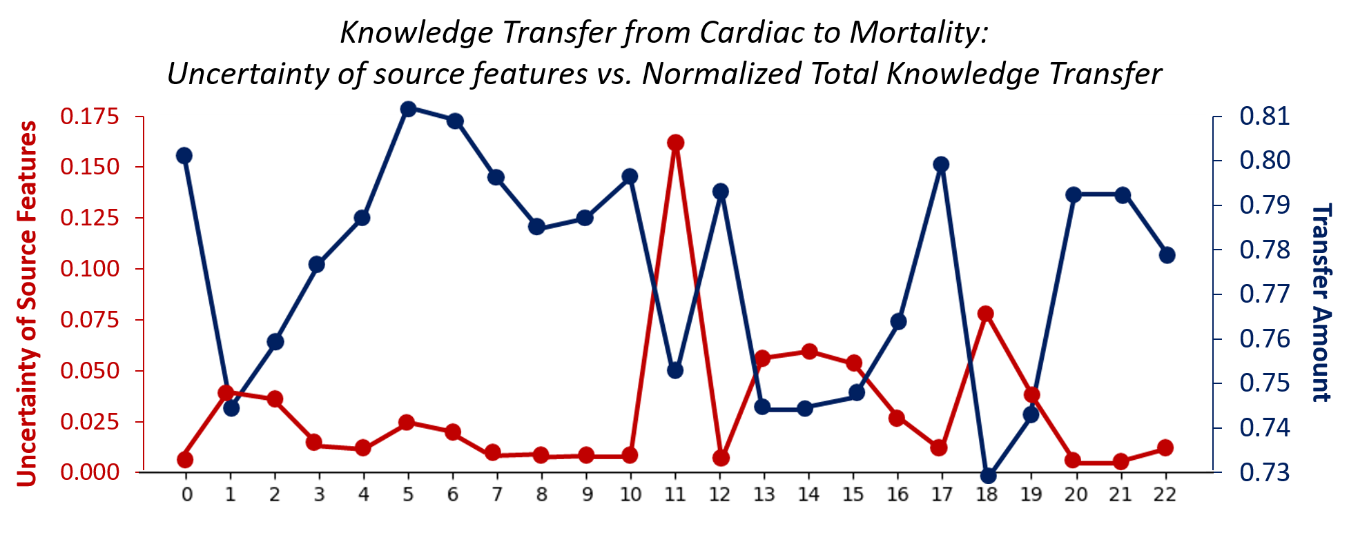
(a) Outgoing Transfer from different Sources

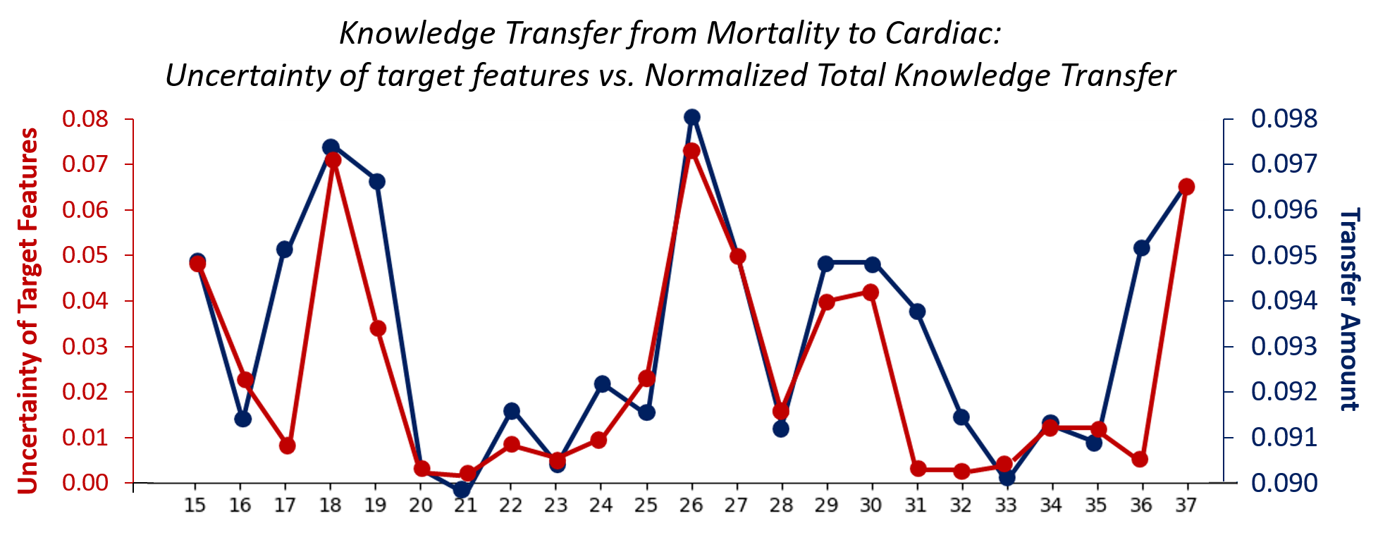
(b) Incoming Transfer to different Targets

Figure 3: Examples showing the relationship between the amount of KT and UC of source and target features. (a) The sources with low UC transfer more knowledge. (b) The targets with high UC receive more knowledge.

We first evaluate the prediction accuracy of the baseline STL and MTL models and ours on the four clinical time-series datasets, by measuring the Area Under the ROC curve (AUROC) (MIMIC-III Infection and PhysioNet (Table 2)). We observe that hard-sharing MTL models outperform STL on some tasks, but suffers from performance degeneration on others (highlighted in red in Table 2), which shows a clear sign of negative transfer. MTL models especially work poorly on MIMIC-III infection, which has clear temporal relationships between tasks. Probabilistic models (e.g., UA [10]) generally outperform their deterministic counterparts (e.g., RETAIN [4]). However, MTL-RETAIN-Kendall [15], which learns the weight for each task loss based on uncertainty, significantly underperforms even the STL-LSTM, which may be due to the fact that losses in our settings are at almost similar scale unlike with the task losses in [15] that have largely different scales. Although the self-attention based model SAnD [31] shows impressive performance on some of the tasks from PhysioNet, it also suffers from performance degeneration in the MTL setting, resulting in lower overall performance. AMTL-LSTM [18] improves on some tasks, but degenerates the performance on the others, which we attribute to the fact that it does not consider inter-timestep transfer. Additionally, AdaCare with dilated convolution showed severely degenerated performance except for one task. On the other hand, our model, TP-AMTL, obtains significant improvements over all STL and MTL baselines on both datasets. It also does not show performance degeneration on any of the tasks, suggesting that it has successfully dealt away with negative transfer in multi-task learning with time-series prediction models. Experimental results on ablation study (regarding inter-, intra-task, future-to-past knowledge transfer, various uncertainty types) and additional two datasets (MIMIC III - Heart Failure and Respiratory Failure) are available in the supplementary file, which further supports our model and shows that our model also generalize well to various, larger datasets.

To further analyze the relationships between uncertainty and knowledge transfer, we visualize knowledge transfer from multiple sources (Figure 3(a)) normalized over the number of targets, and to multiple targets (Figure 3(b)) normalized over the number of sources, along with their uncertainties. Specifically, the uncertainty of a task at a certain timestep is represented by the average of the variance of all feature distributions. The normalized amount of knowledge transfer from task $j$ at time step $t$ to task $d$ is computed as $\scriptstyle{(\alpha^{(t,t)}_{j,d}+\alpha^{(t,t+1)}_{j,d}+...+\alpha^{(t,T)}_{j,d})/(T-t+1)}$. Similarly, the normalized amount of knowledge transfer to task $d$ at time step $t$ from task $j$ is $\scriptstyle{(\alpha^{(1,t)}_{j,d}+\alpha^{(2,t)}_{j,d}+...+\alpha^{(t,t)}_{j,d})/t}$. We observe that source features with low uncertainty transfer knowledge more, while at the target, features with high uncertainty receive more knowledge transfer. However, note that they are not perfectly correlated, since the amount of knowledge transfer is also affected by the pairwise similarities between the source and the target features as well.

Interpretations of the Transfer Weights

Table 3: Clinical Events in selected medical records for case studies. SBP - Systolic arterial blood pressure, DBP - Diastolic arterial blood pressure, BT - Body Temperature, WBC - White Blood Cell Count, FiO2 - Fractional inspired Oxygen, BUN - Blood Urine Nitrogen

		SBP	DBP	BT	WBC	Culture Results				SBP	DBP	Temp	FiO2	Lactate	$HCO_{3}^{-}$	BUN	Creatinine
	1:00	100	53	40.1	12500	N/A			7:38	N/A	37	37	0.35	5.3	N/A	N/A	N/A
	2:57	89	46	N/A	N/A	(+)Klebsiella Pneumoniae			8:38	140	55	36.6	N/A	N/A	10.6	85	4.2
	5:00	120	64	N/A	N/A	N/A			9:38	142	42	N/A	0.4	6.1	N/A	N/A	N/A

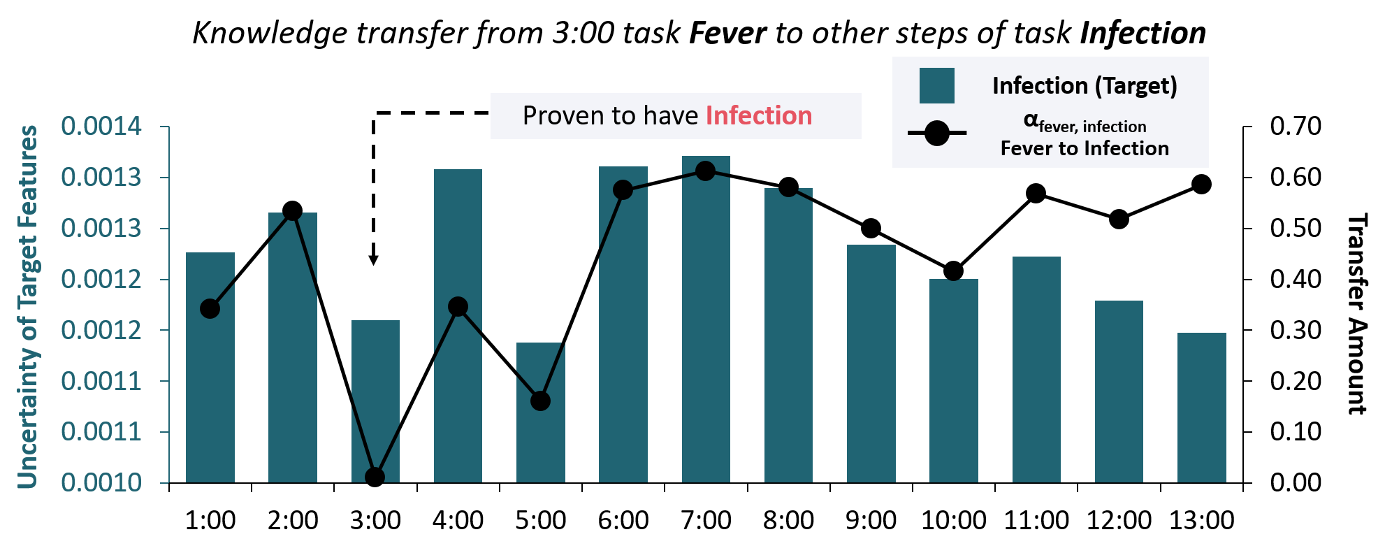
(a) MIMIC-III Infection

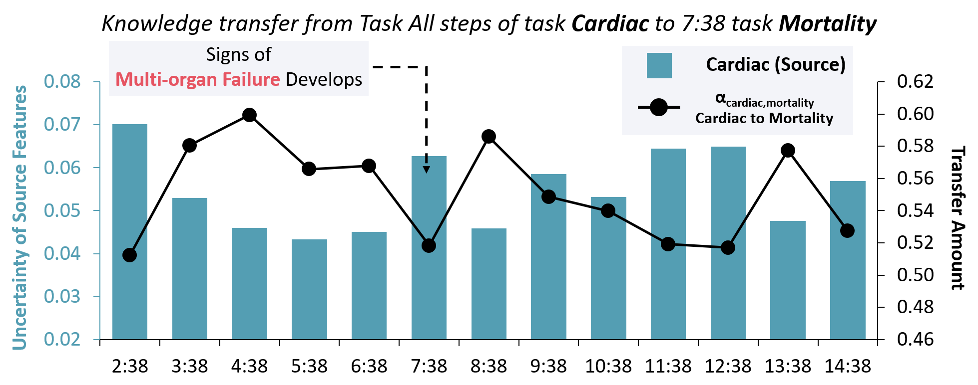
(b) PhysioNet

Figure 4: Visualizations of the amount of UC and normalized KT for example cases where the trends of both UC and KT at certain timesteps are correlated with noticeable clinical events (indicated with dotted arrow).

With the help of a physician, we further analyze how transfer weights and uncertainty are related with the patient’s actual medical conditions (see Table 3 and Figure 4). We first consider an example record of a patient from the MIMIC-III Infection dataset who was suspected of infection on admission, and initially had fever, which was confirmed to be the symptom of bacterial infection later. Figure 4(a) shows the amount of knowledge transfer from task Fever at $3$:$00$ to all later timesteps of task Infection. At this timestep, the patient’s condition changes significantly. We observe that the patient had a fever, and the WBC level has increased to the state of leukocytosis, and both the SBP and DBP decrease over time. Most importantly, the patient is diagnosed to have an infection, as the culture results turns out to be positive for Klebsiella Pneumoniae at 2:57. With the drop of uncertainty of the task Infection around the time window where the event happens (dotted arrow in Figure 4(a)), the amount of knowledge transfer from Fever to Infection drops as well, as the knowledge from the source task becomes less useful.

As for another case study, we consider a record of a patient from PhyisoNet dataset who recovered from cardiac surgery and passed away during admission (Table 3 and Figure 4(b)). From Table 3, we observe that sign of multi-organ failure develops, as features related to respiratory ($FiO_{2}$, $HCO_{3}^{-}$, Lactate), renal (BUN, Creatinine), and cardiac (DBP) function deteriorates. As patient’s condition after surgery gets worse, uncertainty of Cardiac starts to decrease at later timesteps (dotted arrow in Figure 4(b)) and knowledge transfer from Cardiac to Mortality increases as the uncertainty of the source task Cardiac starts to drop, since the knowledge from the source task becomes more reliable. Therefore, by analyzing the learned knowledge graph using our model, we could identify timesteps where meaningful interactions occur between tasks. For more case study examples of MIMIC-III Heart Failure and Respiratory Failure datasets, please see the supplementary file.

Ablation Study

Table 4: Ablation Study result on the MIMIC-III Infection and PhysioNet Dataset.

	MIMIC-III Infection				PhysioNet
Model	Fever	Infection	Mortality	Average	Stay 3	Cardiac	Recovery	Mortality	Average
AMTL-notransfer	0.7048 $\pm$ 0.01	0.6889 $\pm$ 0.01	0.6969 $\pm$ 0.01	0.6968 $\pm$ 0.01	0.8901 $\pm$ 0.01	0.9212 $\pm$ 0.01	0.8986 $\pm$ 0.01	0.7515 $\pm$ 0.01	0.8653 $\pm$ 0.01
AMTL-intratask	0.7082 $\pm$ 0.01	0.7071 $\pm$ 0.01	0.6814 $\pm$ 0.03	0.6989 $\pm$ 0.01	0.8829 $\pm$ 0.01	0.9338 $\pm$ 0.01	0.8812 $\pm$ 0.01	0.7521 $\pm$ 0.01	0.8625 $\pm$ 0.01
AMTL-samestep	0.7130 $\pm$ 0.00	0.6946 $\pm$ 0.01	0.6983 $\pm$ 0.03	0.7019 $\pm$ 0.01	0.8669 $\pm$ 0.01	0.9273 $\pm$ 0.01	0.8902 $\pm$ 0.01	0.7382 $\pm$ 0.01	0.8557 $\pm$ 0.01
TD-AMTL	0.6636 $\pm$ 0.03	0.6874 $\pm$ 0.01	0.6953 $\pm$ 0.02	0.6821 $\pm$ 0.00	0.7381 $\pm$ 0.06	0.9155 $\pm$ 0.01	0.8629 $\pm$ 0.01	0.7365 $\pm$ 0.01	0.8133 $\pm$ 0.02
TP-AMTL (constrained)	0.7159 $\pm$ 0.00	0.7003 $\pm$ 0.01	0.6561 $\pm$ 0.01	0.6908 $\pm$ 0.00	0.8999 $\pm$ 0.01	0.9186 $\pm$ 0.01	0.8892 $\pm$ 0.01	0.7610 $\pm$ 0.01	0.8672 $\pm$ 0.00
TP-AMTL (epistemic)	0.6997 $\pm$ 0.01	0.7196 $\pm$ 0.00	0.7106 $\pm$ 0.02	0.7100 $\pm$ 0.01	0.8952 $\pm$ 0.01	0.9341 $\pm$ 0.01	0.8934 $\pm$ 0.01	0.7547 $\pm$ 0.01	0.8693 $\pm$ 0.01
TP-AMTL (aleatoric)	0.6984 $\pm$ 0.02	0.7032 $\pm$ 0.01	0.7217 $\pm$ 0.02	0.7078 $\pm$ 0.00	0.8012 $\pm$ 0.03	0.9183 $\pm$ 0.01	0.8537 $\pm$ 0.02	0.7401 $\pm$ 0.03	0.8283 $\pm$ 0.01
TP-AMTL (full model)	0.7165 $\pm$ 0.00	0.7093 $\pm$ 0.01	0.7098 $\pm$ 0.01	0.7119 $\pm$ 0.00	0.8953 $\pm$ 0.01	0.9416 $\pm$ 0.01	0.9016 $\pm$ 0.01	0.7586 $\pm$ 0.01	0.8743 $\pm$ 0.01

We compare our model against several variations of our model with varying knowledge transfer direction with respect to task (inter-task) and time (inter-timestep), and with temporal constraint (only future-to-past). Also we examine two kinds of uncertainty (epistemic, aleatoric) with our model (Table 4).

Inter-task and inter-timestep knowledge transfer.

1) AMTL-notransfer: The variant of our model without knowledge transfer.
2) AMTL-intratask: The variant of our model that knowledge only transfers within a same task.
3) AMTL-samestep: Another variant of our model that knowledge transfers only within a same time-step.
4) TD-AMTL: The deterministic counterpart of our model.

Our model outperforms AMTL-intratask and AMTL-samestep, which demonstrates the effectiveness of inter-task and inter-step knowledge transfer (Table 4). TD-AMTL largely underperforms any variants, which may be due to overfitting of the knowledge transfer model, that can be effectively prevented by our bayesian framework.

Future-to-past transfer.

5) TP-AMTL (constrained): the model with temporal constraint

The unconstrained model outperforms TP-AMTL (constrained) (Table 4), where transfer can only happen from the later timestep to earlier ones.

Two kinds of uncertainty.

6) TP-AMTL (epistemic) uses only MC-dropout to model epistemic uncertainty and $p_{\theta}(\mathbf{z}_{d}|\mathbf{x},\bm{\omega})$ is simplified into $\mathcal{N}\left(\mathbf{z}_{d};\bm{\mu}_{d},\bm{0}\right)$ (i.e. its pdf becomes the dirac delta function at $\bm{\mu}_{d}$ and $\mathbf{z}_{d}$ is always $\bm{\mu}_{d}$)
7) TP-AMTL (aleatoric) uses only $p_{\theta}(\mathbf{z}_{d}|\mathbf{x},\bm{\omega})$ to model the aleatoric uncertainty, without MC-dropout.

For both MIMIC-III and PhysioNet datasets, epistemic uncertainty attributes more to the performance gain (Table 4). However, it should be noted that the impacts of two kinds of uncertainty vary from dataset to dataset. By modelling both kinds of uncertainty, the model is guaranteed to get the best performance.

Conclusion

We propose a novel probabilistic asymmetric multi-task learning framework that allows asymmetric knowledge transfer between tasks at different timesteps, based on the uncertainty. While existing asymmetric multi-task learning methods consider asymmetric relationships between tasks as fixed, the task relationship may change at different timesteps in time-series data. Moreover, knowledge obtained for a task at a specific timestep could be useful for other tasks in later timesteps. Thus, to model the varying direction of knowledge transfer and across-timestep knowledge transfer, we propose a novel probabilistic multi-task learning framework that performs knowledge transfer based on the uncertainty of the latent representations for each task and timestep. We validate our model on clinical time-series prediction tasks on four datasets, on which our model shows strong performance over the baseline symmetric and asymmetric multi-task learning models, without any sign of negative transfer. Several case studies with learned knowledge graphs show that our model is interpretable, providing useful and reliable information on model predictions. This interpretability of our model will be useful in building a safe time-series analysis system for large-scale settings where both the number of time-series data instances and timestep are extremely large, such that manual analysis is impractical.

Detailed Description of Datasets and Experimental Setup

Datasets and Tasks

Here we include detailed feature information of PhysioNet dataset and explanation on MIMIC III-Respiratory failure and MIMIC III-Heart Failure.

MIMIC III [12]-Infection

Here we include the configuration of MIMIC III-Infection dataset for reference (Figure 5).

Figure 5: MIMIC III-Infection: Task overview. Tasks used in the experiment included the diagnostic process of the patient infectious status. When a patient in ICU is infected with any of the pathogens, body temperature elevates (Fever (Task 1)) as a sign of infection. Next, Infection (Task 2), is confirmed when the blood culture result turns out to be positive with bacteria, fungus, or virus. Lastly, Mortality (Task 3) can be resulted from infection.

PhysioNet

[5] (Figure 6) We list 29 pre-selected physiological signs in this section: age, gender, height, weight, Systolic Blood Pressure, Diastolic Blood Pressure, mean arterial pressure, heart rate, respiratory rate, body temperature, glucose, bilirubin, serum electrolytes (sodium, potassium, magnesium, bicarbonate), lactate, pH, Hematocrit, platelets, Partial Pressure of Oxygen (PaO₂), Partial Pressure of carbon dioxide (PaCO₂), Oxygen Saturation (SaO₂), Fraction of Inspired Oxygen (FiO₂), Glasgow Coma Scale (GCS), blood urea nitrogen (BUN), Creatinine, Urine, Mechanical Ventilation Status.

Figure 6: PhysioNet : Task overview. Tasks generated from PhysioNet dataset including three tasks that have temporal relationship with task Mortality (Task 3). Shorter length of stay in ICU (Stay $<3$ (Task 1)) has reverse temporal relationship with Mortality. Also, patient condition related to surgical operation(Cardiac (Task 2) surgery, and general surgery (Recovery (Task 3))) are temporally related to Mortality.

To test the generalization performance of our model, we compiled two additional datasets, namely Heart Failure and Respiratory Failure, out of the MIMIC III dataset [12].

MIMIC III-Heart Failure

From the MIMIC III dataset, we collected $3,577$ data instances, each of which corresponds to the record of a patient (age between 18 and 100) admitted to the ICU of a hospital. This dataset contains 15 features which are associated to the risk of heart failure occurrence, including Heart rate (HR), Systolic Blood Pressure (SBP), Diastolic Blood Pressure (DBP), Body Temperature (BT), Fraction of inspired oxygen (FiO₂), Mixed venous oxygen saturation (M_vO₂), Oxygen Saturation of arterial blood (S_aO₂), Brain natriuretic peptide (BNP), Ejection Fraction (EF), Glasgow Coma scale (GCS) - Verbal, Motor, Eye. We considered four tasks that might lead to heart failure. The first task (Ischemic) is the patient condition where a patient is diagnosed with ischemic heart disease. The second task (Valvular) is related to the diagnosis of valvular heart disease, and the third task (Heart Failure) contains the condition where a patient is diagnosed with various types of heart failure. Lastly, Mortality (Task 4) can be a possible outcome of heart failure. We used random split of approximately 1850/925/925 instances for train, valid, test set. ICD code for the diagnosis of each disease is summarized in Table 13 and Table 14 summarizes all feature information used to construct this dataset.

Figure 7: MIMIC III-Heart Failure: Task overview. Tasks used in the experiment include the tasks that are temporally related. The first and second tasks Ischemic (Ischemic Heart Disease, Task 1) and Valvular (Valvular Heart Disease, Task 2) can both result in Heart Failure (Task 3) of a patient. Also, Mortality (Task4) is one possible outcome of Heart Failure.

MIMIC III-Respiratory Failure

We collected total of $37,818$ distinct ICU admissions of adult patients, between the age of 18 and 100. To further test the generalization performance of our model to larger dataset, we test the model performance on three partial datasets. First we run the experiment with full admission instances sampled for 48 hours after admission (Table 7), full $37,818$ instances of data sampled for 48 hours (Table 8). The disease and clinical event label, ICD code and item ID are summarized in Table  15. This dataset contains 29 features, which are predictive of respiratory failure occurrence, including Fraction of inspired oxygen (Fi$O_{2}$), Oxygen Saturation of arterial blood ($S_{a}$O₂) and venous blood ($S_{v}O_{2}$), Partial Pressure of oxygen in alveoli ($P_{A}O_{2}$), Arterial/Venous oxygen content ($C_{a}O_{2}$), which is summarized in Table 16. Tasks considered in this task includes four respiratory conditions that are required for the prediction of respiratory failure (Task 5) and mortality (Task 7) (Table 15): Hypoxemia (Task1, $P_{a}O_{2}<60mmHg$), Hypercapnia (Task2, $P_{a}CO_{2}>50mmHg$), VQ Mismatch (Task 3, $A_{a}DO_{2}>10$), Acidosis (Task 4, $pH<7.35$), Respiratory Failure (Task 5), Cyanosis (Task 6, $S_{a}O_{2}<60mmHg$). The collected dataset was randomly split into $26,472$/$5,672$/$5,674$ for training/validation/test in full dataset, and $2,800$/$600$/$600$ for total $4,000$ instances.

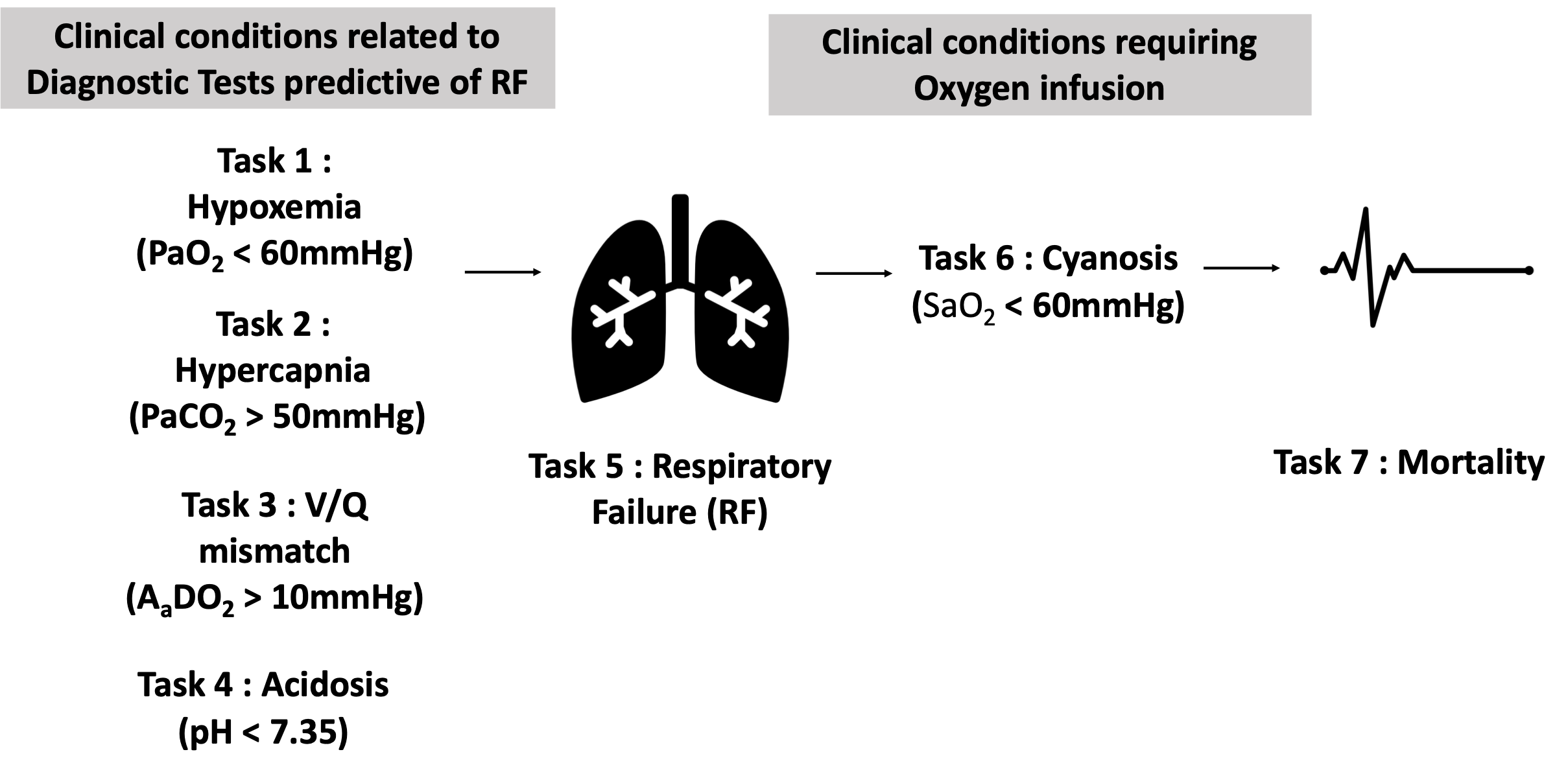
Figure 8: MIMIC III-Respiratory Failure: Task overview. Tasks used in the experiment includes the tasks that are 1) clinical conditions related to diagnostic tests of respiratory failure (Hypoxemia (Task 1), Hypercarbia (Task 2), V/Q mismatch (Task 3), and Acidosis (Task 4)), 2) Respiratory Failure (Task 5), 3) clinical condition related to treatment planning of patients (Cyanosis (Task 6)), 4) Mortality (Task 7).

Baselines

STL-LSTM.

The single- and multi-task learning method which uses RNNs to capture the temporal dependencies.

MTL-LSTM.

The naive hard-sharing multi-task learning method where all tasks share the same network except for the separate output layers for prediction, whose base network is Long Short-Term Memory Network (LSTM).

$$(\mathbf{v}_{d}^{(1)},\mathbf{v}_{d}^{(2)},...,\mathbf{v}_{d}^{(T)})=\mathbf{v}_{d}=\mathbf{x}\mathbf{W}^{d}_{emb}\in\mathbbm{R}^{T\times k}$$

$$(\mathbf{h}_{d}^{(1)},\mathbf{h}_{d}^{(2)},...,\mathbf{h}_{d}^{(T)})=LSTM_{d}(\mathbf{v}_{d}^{(1)},\mathbf{v}_{d}^{(2)},...,\mathbf{v}_{d}^{(T)})$$

$$\beta_{d}^{(t)}=\tanh{(\bm{h}_{d}^{(t)})}$$

$$p(\widehat{y_{d}}|\mathbf{x})=Sigmoid\left(\frac{1}{T}\left({\sum}_{t=1}^{T}\beta_{d}^{(t)}\odot\mathbf{v}^{(t)}\right)\mathbf{W}_{d}^{o}+b_{d}^{o}\right)$$

STL/MTL-Transformer

The single-task learning method which uses Transformer architecture [33] to capture the temporal dependencies:

$$\mathbf{v}=\mathbf{x}\mathbf{W}_{emb}+POS\_ENC\in\mathbbm{R}^{T\times k}$$

$$\mathbf{f}_{d}=TRANS\_BLOCK_{d}(v)\in\mathbbm{R}^{T\times k}$$

$$\mathbf{c}_{d}=\frac{1}{T}(\mathbf{f}_{d}^{(1)}+\mathbf{f}_{d}^{(2)}+...+\mathbf{f}_{d}^{(T)})$$

$$p(\widehat{y_{d}}|\mathbf{x})=Sigmoid\left(\mathbf{c}_{i}\mathbf{W}_{d}^{o}+b_{d}^{o}\right)$$

where $POS\_ENC$ is the positional encoding used in Transformer, $TRANS\_BLOCK$ is also the architecture used in the paper, which consists of two sublayers: $MULTI\_HEAD$ (with four heads) and $FFW$. We also used residual connection and layer norm after each sublayer as in the original paper.

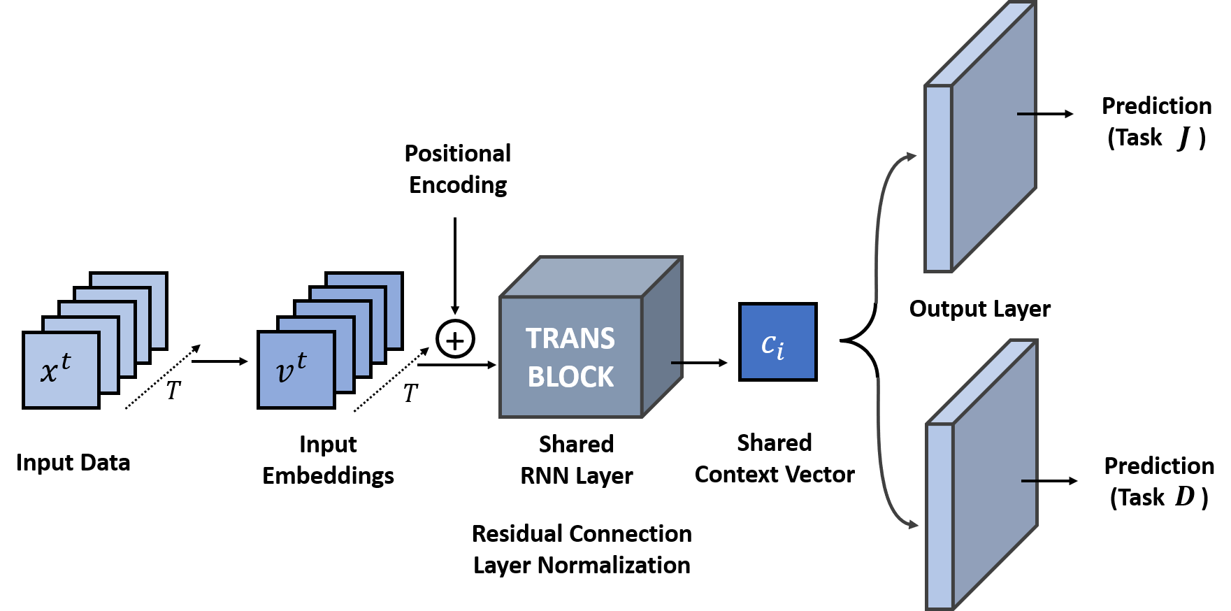
Figure 10: Multi Task Learning with Transformer

MTL-RETAIN.

The same as MTL-LSTM, but with RETAIN[4] as the base network. Specifically, after getting the shared context vector $\mathbf{c}_{i}$, separated output layers will be applied to form the prediction for each task.

MTL-UA.

The same as MTL-LSTM, but with UA[10] as the base network. Specifically, after getting the shared context vector $\mathbf{c}_{i}$, separated output layers will be applied to form the prediction for each task. This can be seen as the probabilistic version of MTL-RETAIN.

$$\mathbf{c}_{i}:\text{context vector from RETAIN, UA}$$ (13)

$$p(\widehat{y_{d}}|\mathbf{x})=Sigmoid\left(\mathbf{c}_{i}\mathbf{W}_{d}^{o}+b_{d}^{o}\right)$$ (14)

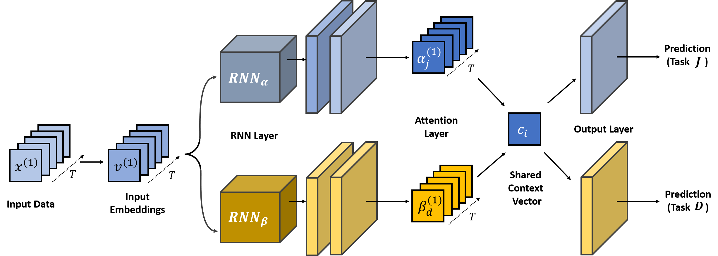
Figure 11: Multi Task Learning with RETAIN, UA model

AMTL-LSTM.

This is asymmetric multi-task learning [18] adopted for our time-series prediction framework, where we learn the knowledge transfer graph between task-specific parameters, which is learned to perform asymmetric knowledge transfer based on the task loss. The parameters for each task are shared across all timesteps, which will result in static asymmetric transfer between tasks.

MTL-RETAIN-Kendall

This model is similar to MTL-RETAIN. However, we followed the uncertainty-aware loss weighting scheme from [15] to weight the loss for each task by its uncertainty:

$${\sum}_{d=1}^{D}{\left(\frac{1}{\sigma_{d}^{2}}L_{d}+log(\sigma_{d})\right)}$$ (15)

TP-AMTL.

Our probabilistic temporal asymmetric multi-task learning model that performs both intra-task and inter-task knowledge transfer.

Details of models in Ablation study

AMTL-intratask.

The probabilistic AMTL model with uncertainty-aware knowledge transfer, but performs knowledge transfer only within the same task at the transfer layer. Note that, however, this model can still share inter-task knowledge in a symmetrical manner since it still has shared lower layers (the embedding and the LSTM layers).

$$\mathbf{C}_{d}^{(t)}=\mathbf{f}_{d}^{(t)}+{\sum}_{i=1}^{t}\alpha^{(i,t)}_{d,d}*G_{d}\left(\mathbf{f}_{d}^{(i)}\right)\forall t\in\{1,2,...,T\}$$ (16)

AMTL-samestep.

The probabilistic model with uncertainty-aware knowledge transfer, which performs knowledge transfer only between the features at the same timestep, at the transfer layer. Again, note that this model can still capture the temporal dependencies among the timesteps to certain degree, as it has shared lower layers.

$$\mathbf{C}_{d}^{(t)}=\mathbf{f}_{d}^{(t)}+{\sum}^{D}_{j=1}G_{j,d}\left(\mathbf{f}_{j}^{(t)}\right)\forall t\in\{1,2,...,T\}$$ (17)

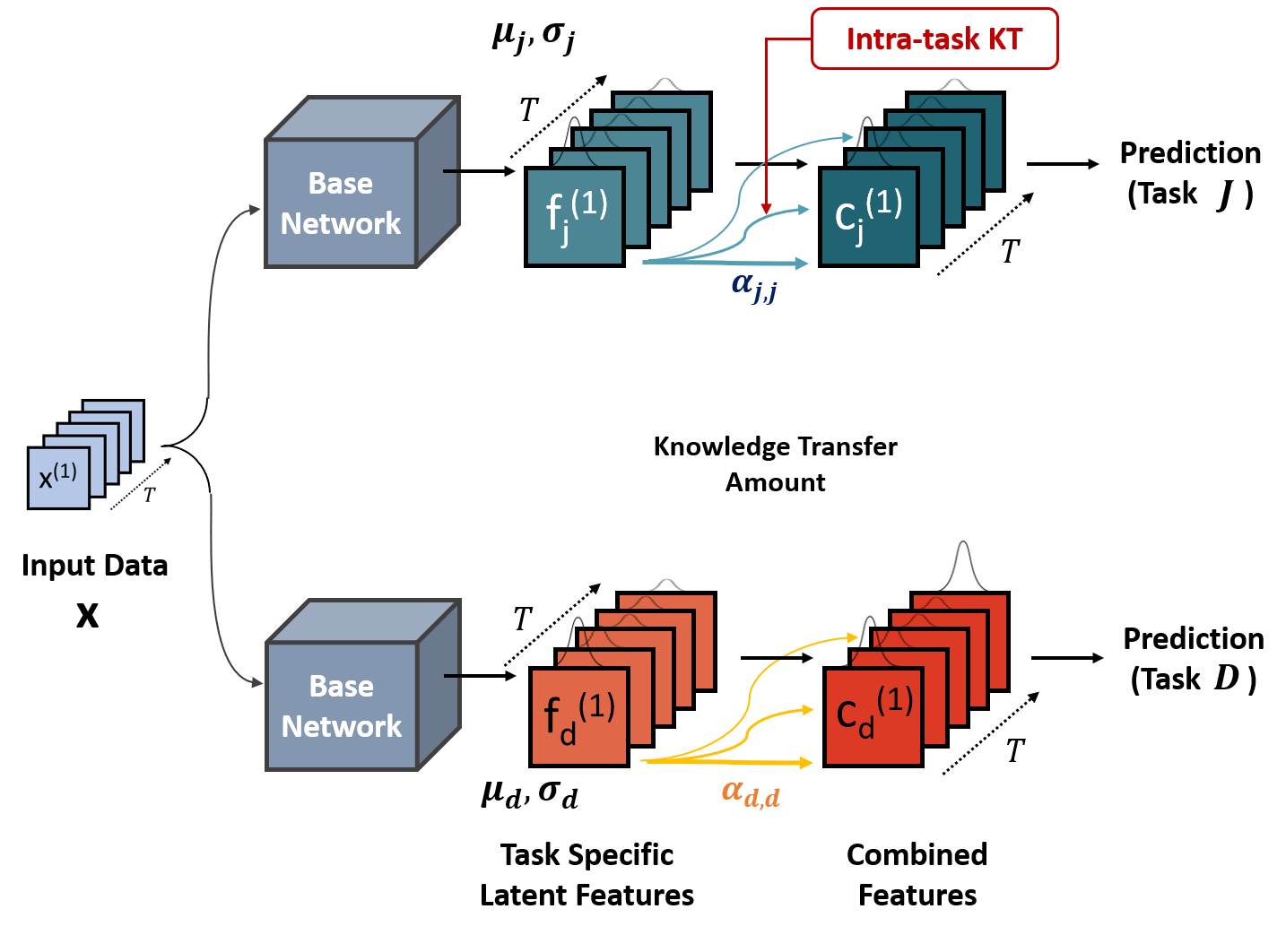
(a) Intratask Knowledge Transfer

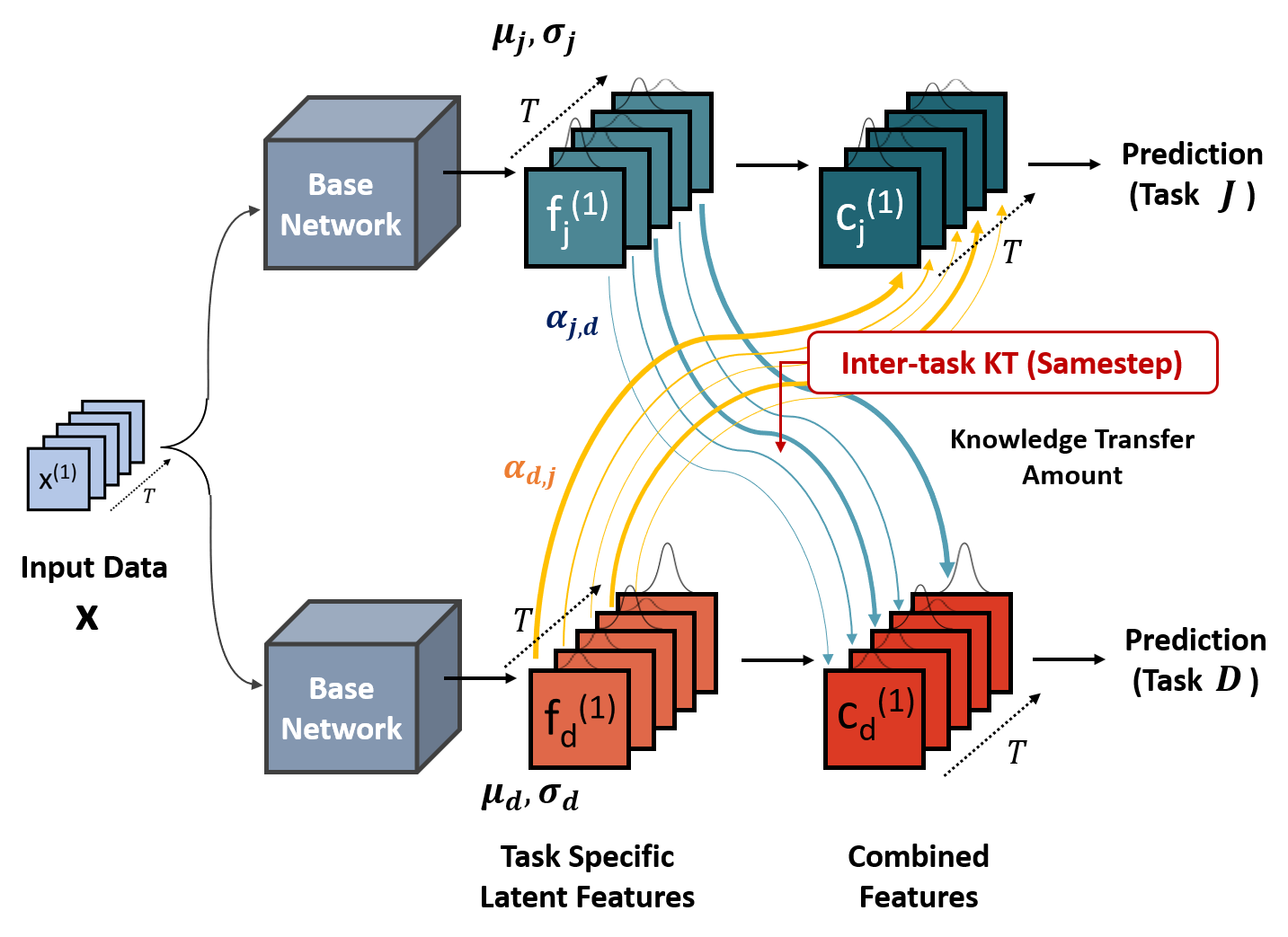
(b) Samestep Knowledge Transfer

Figure 12: Asymmetric Multi Task Learning with (a) Intratask Knowledge Transfer and (b) Samestep Knowledge Transfer

TD-TAMTL.

The deterministic version of our model that does not make use of feature-level uncertainty when performing knowledge transfer.

$$\mathbf{v}=\mathbf{x}\mathbf{W}_{emb}\in\mathbbm{R}^{T\times k}$$

$$\mathbf{h}=(\mathbf{h}^{(1)},\mathbf{h}^{(2)},...,\mathbf{h}^{(T)})=RNN(\mathbf{v}^{(1)},\mathbf{v}^{(2)},...,\mathbf{v}^{(T)})$$

$$\mathbf{h}_{d}=\sigma((...\sigma(\sigma(\mathbf{h}\mathbf{W}^{1}_{d}+\mathbf{b}^{1}_{d})\mathbf{W}^{2}_{d}+\mathbf{b}^{2}_{d})...)\mathbf{W}^{L}_{d}+\mathbf{b}^{L}_{d})$$

$$(\mathbf{f}_{d}^{(1)},\mathbf{f}_{d}^{(2)},...,\mathbf{f}_{d}^{(T)})=\mathbf{h}_{d}\in\mathbbm{R}^{T\times k}$$

$$\mathbf{C}_{d}^{(t)}=\mathbf{f}_{d}^{(t)}+{\sum}^{D}_{j=1}{\sum}_{i=1}^{t}\alpha^{(i,t)}_{j,d}*G\left(\mathbf{f}_{j}^{(i)}\right)$$

$$\forall t\in\{1,2,...,T\}$$

$$\bm{\beta}_{d}^{(t)}=tanh\left(\mathbf{C}_{d}^{(t)}\mathbf{W}_{d}^{\beta}+\mathbf{b}_{d}^{\beta}\right)\quad\forall t\in\{1,2,...,T\}$$

$$p(\widehat{y_{d}}|\mathbf{x})=Sigmoid\left(\frac{1}{T}\left({\sum}_{t=1}^{T}\beta_{d}^{(t)}\odot\mathbf{v}^{(t)}\right)\mathbf{W}_{d}^{o}+b_{d}^{o}\right)$$

where $\alpha^{(i,t)}_{j,d}=F_{\theta}(\mathbf{f}_{f}^{(i)},\mathbf{f}_{d}^{(t)})$

TP-TAMTL - no constraints.

$$\mathbf{C}_{d}^{(t)}=\mathbf{f}_{d}^{(t)}+{\sum}^{D}_{j=1}{\sum}_{i=1}^{T}\alpha^{(i,t)}_{j,d}*G_{j,d}\left(\mathbf{f}_{j}^{(i)}\right)$$

$$\forall t\in\{1,2,...,T\}$$

Configuration and Hyperparameters

We trained all the models using Adam optimizer. We set the maximum iteration for Adam optimizer as 100,000, and for other hyper-parameters, we searched for the optimal values by cross-validation, within predefined ranges as follows: Hidden units: {8, 16, 32, 64}, number of layers: {2,3,6}, mini batch size: {32, 64, 128, 256}, learning rate: {0.01, 0.001, 0.0001}, L2 regularization: {0.02, 0.002, 0.0002}, and dropout rate: {0.1, 0.15, 0.2, 0.25, 0.3, 0.4, 0.5}.

Time Complexity of the model

The complexity of each baselines and our final model is summarized in Table 5.

Table 5: Complexity of the Baseline Models

Models	Complexity
Transformer [33]	$O(T^{2})$
RETAIN [4]	$O(T)$
UA [10]	$O(T)$
SAnD [31]	$O(T^{2})$
TP-AMTL (ours)	$O(T)$

Table 6: MIMIC-III Heart Failure. The reported numbers are average AUROC and standard error over five runs. The numbers colored in red for MTL models denote accuracies lower than those of their STL counterparts.

Models		Tasks
		Ischemic	Valvular	Heart Failure	Mortality	Average
	LSTM	0.7072 $\pm$ 0.01	0.7700 $\pm$ 0.02	0.6899 $\pm$ 0.02	0.7169 $\pm$ 0.03	0.7210 $\pm$ 0.01
	Transformer[33]	0.6877 $\pm$ 0.01	0.7655 $\pm$ 0.01	0.7062 $\pm$ 0.01	0.7183 $\pm$ 0.03	0.7194 $\pm$ 0.01
STL	RETAIN [4]	0.6573 $\pm$ 0.03	0.7875 $\pm$ 0.01	0.6850 $\pm$ 0.01	0.7027 $\pm$ 0.02	0.7081 $\pm$ 0.01
	UA [10]	0.6843 $\pm$ 0.01	0.7728 $\pm$ 0.02	0.7090 $\pm$ 0.01	0.7191 $\pm$ 0.01	0.7213 $\pm$ 0.01
	SAnD[31]	0.7083 $\pm$ 0.01	0.7995 $\pm$ 0.01	0.7245 $\pm$ 0.01	0.7438 $\pm$ 0.01	0.7440 $\pm$ 0.01
	AdaCare[21]	0.6274 $\pm$ 0.02	0.7509 $\pm$ 0.01	0.6496 $\pm$ 0.02	0.6775 $\pm$ 0.01	0.6764 $\pm$ 0.01
	LSTM	0.6838 $\pm$ 0.02	0.7808 $\pm$ 0.02	0.6965 $\pm$ 0.01	0.7093 $\pm$ 0.02	0.7254 $\pm$ 0.02
	TRANS[33]	0.6801 $\pm$ 0.01	0.7693 $\pm$ 0.01	0.7098 $\pm$ 0.02	0.7008 $\pm$ 0.02	0.7150 $\pm$ 0.02
MTL	RETAIN	0.6649 $\pm$ 0.01	0.7532 $\pm$ 0.03	0.6868 $\pm$ 0.02	0.7023 $\pm$ 0.03	0.7018 $\pm$ 0.02
	UA	0.6917 $\pm$ 0.01	0.7868 $\pm$ 0.01	0.7073 $\pm$ 0.01	0.7029 $\pm$ 0.01	0.7222 $\pm$ 0.01
	SAnD[31]	0.7206 $\pm$ 0.01	0.8036 $\pm$ 0.01	0.7169 $\pm$ 0.01	0.7369 $\pm$ 0.01	0.7445 $\pm$ 0.01
	AdaCare[21]	0.6261 $\pm$ 0.03	0.6937 $\pm$ 0.01	0.6466 $\pm$ 0.02	0.6059 $\pm$ 0.02	0.6431 $\pm$ 0.02
	RETAIN-Kendall	0.6476 $\pm$ 0.03	0.7712 $\pm$ 0.02	0.6826 $\pm$ 0.01	0.7017 $\pm$ 0.02	0.7008 $\pm$ 0.01
	AMTL-LSTM[18]	0.6963 $\pm$ 0.01	0.7997 $\pm$ 0.02	0.7006 $\pm$ 0.01	0.7108 $\pm$ 0.01	0.7268 $\pm$ 0.01
	TP-AMTL (our model)	0.7113 $\pm$ 0.01	0.7979 $\pm$ 0.01	0.7103 $\pm$ 0.01	0.7185 $\pm$ 0.02	0.7345 $\pm$ 0.01

Table 7: MIMIC-III Respiratory Failure (RF). The reported numbers are average AUROC and standard error over five runs. The numbers colored in red for MTL models denote accuracies lower than those of their STL counterparts.

Models		Tasks
		Hypoxemia	Hypercapnia	VQ Mismatch	Acidosis	RF	Cyanosis	Mortality	Average
	LSTM	0.7679 $\pm$ 0.01	0.7278 $\pm$ 0.02	0.8032 $\pm$ 0.02	0.8916 $\pm$ 0.01	0.7127 $\pm$ 0.02	0.6447 $\pm$ 0.02	0.8038 $\pm$ 0.01	0.7645 $\pm$ 0.03
	Transformer [33]	0.7573 $\pm$ 0.02	0.7326 $\pm$ 0.01	0.8406 $\pm$ 0.02	0.8919 $\pm$ 0.00	0.7750 $\pm$ 0.05	0.8001 $\pm$ 0.01	0.7069 $\pm$ 0.03	0.7863 $\pm$ 0.01
STL	RETAIN [4]	0.7695 $\pm$ 0.01	0.753 $\pm$ 0.01	0.8708 $\pm$ 0.01	0.8549 $\pm$ 0.03	0.7552 $\pm$ 0.01	0.6743 $\pm$ 0.01	0.8060 $\pm$ 0.01	0.7834 $\pm$ 0.02
	UA [10]	0.7494 $\pm$ 0.03	0.7469 $\pm$ 0.02	0.8931 $\pm$ 0.02	0.8975 $\pm$ 0.01	0.7873 $\pm$ 0.03	0.7069 $\pm$ 0.03	0.7970 $\pm$ 0.01	0.7959 $\pm$ 0.01
	SAnD [31]	0.7919 $\pm$ 0.01	0.7431 $\pm$ 0.01	0.8868 $\pm$ 0.04	0.9086 $\pm$ 0.01	0.7824 $\pm$ 0.03	0.8212 $\pm$ 0.00	0.7075 $\pm$ 0.02	0.8059 $\pm$ 0.01
	AdaCare[21]	0.6593 $\pm$ 0.02	0.7062 $\pm$ 0.02	0.7793 $\pm$ 0.01	0.8590 $\pm$ 0.01	0.6935 $\pm$ 0.04	0.7500 $\pm$ 0.02	0.6643 $\pm$ 0.04	0.7302 $\pm$ 0.04
	LSTM	0.7826 $\pm$ 0.00	0.7476 $\pm$ 0.01	0.8880 $\pm$ 0.01	0.8937 $\pm$ 0.00	0.7948 $\pm$ 0.02	0.6992 $\pm$ 0.01	0.8030 $\pm$ 0.01	0.8013 $\pm$ 0.01
	TRANS [33]	0.7778 $\pm$ 0.01	0.7537 $\pm$ 0.01	0.8717 $\pm$ 0.02	0.8913 $\pm$ 0.00	0.7862 $\pm$ 0.01	0.7341 $\pm$ 0.04	0.8036 $\pm$ 0.01	0.8026 $\pm$ 0.01
	RETAIN [4]	0.7902 $\pm$ 0.01	0.7377 $\pm$ 0.01	0.8835 $\pm$ 0.02	0.902 $\pm$ 0.00	0.7726 $\pm$ 0.01	0.7246 $\pm$ 0.04	0.8106 $\pm$ 0.01	0.8030 $\pm$ 0.01
MTL	RETAIN-Kendall [15]	0.7759 $\pm$ 0.01	0.7546 $\pm$ 0.01	0.8714 $\pm$ 0.03	0.8949 $\pm$ 0.01	0.7953 $\pm$ 0.02	0.6789 $\pm$ 0.02	0.7739 $\pm$ 0.01	0.7921 $\pm$ 0.01
	UA [10]	0.7646 $\pm$ 0.03	0.7479 $\pm$ 0.00	0.9271 $\pm$ 0.01	0.8935 $\pm$ 0.00	0.7623 $\pm$ 0.03	0.6952 $\pm$ 0.02	0.7891 $\pm$ 0.01	0.7971 $\pm$ 0.01
	SAnD [31]	0.7889 $\pm$ 0.01	0.7402 $\pm$ 0.01	0.9000 $\pm$ 0.02	0.9066 $\pm$ 0.01	0.7683 $\pm$ 0.03	0.8157 $\pm$ 0.02	0.7240 $\pm$ 0.03	0.8062 $\pm$ 0.02
	AdaCare[21]	0.6991 $\pm$ 0.04	0.6357 $\pm$ 0.04	0.7907 $\pm$ 0.06	0.8236 $\pm$ 0.02	0.7189 $\pm$ 0.04	0.6972 $\pm$ 0.03	0.6987 $\pm$ 0.02	0.7234 $\pm$ 0.01
	AMTL-LSTM [18]	0.7577 $\pm$ 0.02	0.7436 $\pm$ 0.01	0.8667 $\pm$ 0.04	0.9049 $\pm$ 0.00	0.7246 $\pm$ 0.03	0.6928 $\pm$ 0.03	0.8073 $\pm$ 0.00	0.7854 $\pm$ 0.01
	TP-AMTL (our model)	0.7943 $\pm$ 0.01	0.7786 $\pm$ 0.02	0.9322 $\pm$ 0.00	0.9113 $\pm$ 0.01	0.7962 $\pm$ 0.01	0.7894 $\pm$ 0.02	0.819 $\pm$ 0.02	0.8316 $\pm$ 0.01

Table 8: MIMIC-III Respiratory Failure (RF) - $37,818$ instances. The reported numbers are average AUROC and standard error over five runs. The numbers colored in red for MTL models denote accuracies lower than those of their STL counterparts.

Models		Tasks
		Hypoxemia	Hypercapnia	VQ Mismatch	Acidosis	RF	Cyanosis	Mortality	Average
	LSTM	0.7857 $\pm$ 0.01	0.7899 $\pm$ 0.00	0.9248 $\pm$ 0.00	0.9203 $\pm$ 0.00	0.811 $\pm$ 0.01	0.8333 $\pm$ 0.02	0.8432 $\pm$ 0.01	0.8440 $\pm$ 0.05
	Transformer [33]	0.7863 $\pm$ 0.01	0.7808 $\pm$ 0.00	0.9110 $\pm$ 0.01	0.9286 $\pm$ 0.00	0.8029 $\pm$ 0.01	0.8140 $\pm$ 0.01	0.8416 $\pm$ 0.00	0.8379 $\pm$ 0.00
STL	RETAIN [4]	0.7968 $\pm$ 0.00	0.7802 $\pm$ 0.00	0.9276 $\pm$ 0.00	0.9219 $\pm$ 0.00	0.8120 $\pm$ 0.00	0.8253 $\pm$ 0.01	0.8503 $\pm$ 0.01	0.8449 $\pm$ 0.05
	UA [10]	0.8315 $\pm$ 0.01	0.8271 $\pm$ 0.00	0.846 $\pm$ 0.02	0.8002 $\pm$ 0.02	0.8020 $\pm$ 0.01	0.8304 $\pm$ 0.01	0.8651 $\pm$ 0.00	0.8432 $\pm$ 0.04
	SAnD [31]	0.8195 $\pm$ 0.04	0.7864 $\pm$ 0.00	0.9341 $\pm$ 0.00	0.9324 $\pm$ 0.00	0.8214 $\pm$ 0.01	0.8617 $\pm$ 0.00	0.8565 $\pm$ 0.01	0.8589 $\pm$ 0.01
	AdaCare[21]	0.6511 $\pm$ 0.01	0.6673 $\pm$ 0.00	0.7817 $\pm$ 0.02	0.7588 $\pm$ 0.01	0.7394 $\pm$ 0.02	0.7089 $\pm$ 0.01	0.6734 $\pm$ 0.03	0.7115 $\pm$ 0.01
	LSTM	0.8021 $\pm$ 0.00	0.7843 $\pm$ 0.00	0.8968 $\pm$ 0.05	0.9197 $\pm$ 0.00	0.816 $\pm$ 0.00	0.8261 $\pm$ 0.01	0.8453 $\pm$ 0.00	0.8414 $\pm$ 0.05
	Transformer [33]	0.7937 $\pm$ 0.00	0.7781 $\pm$ 0.00	0.9247 $\pm$ 0.00	0.9234 $\pm$ 0.00	0.8231 $\pm$ 0.00	0.8139 $\pm$ 0.00	0.8330 $\pm$ 0.00	0.8414 $\pm$ 0.05
MTL	RETAIN	0.7992 $\pm$ 0.00	0.7794 $\pm$ 0.00	0.9346 $\pm$ 0.00	0.9199 $\pm$ 0.00	0.8139 $\pm$ 0.01	0.824 $\pm$ 0.00	0.8313 $\pm$ 0.01	0.8432 $\pm$ 0.06
	UA	0.8316 $\pm$ 0.00	0.8103 $\pm$ 0.00	0.943 $\pm$ 0.00	0.9354 $\pm$ 0.00	0.8397 $\pm$ 0.00	0.8727 $\pm$ 0.00	0.8754 $\pm$ 0.00	0.8726 $\pm$ 0.05
	RETAIN-Kendall	0.8028 $\pm$ 0.00	0.7794 $\pm$ 0.00	0.9274 $\pm$ 0.00	0.9168 $\pm$ 0.00	0.8207 $\pm$ 0.00	0.8117 $\pm$ 0.00	0.8352 $\pm$ 0.01	0.8420 $\pm$ 0.05
	SAnD [31]	0.8253 $\pm$ 0.00	0.8108 $\pm$ 0.00	0.9421 $\pm$ 0.00	0.9355 $\pm$ 0.00	0.8366 $\pm$ 0.01	0.8646 $\pm$ 0.00	0.8593 $\pm$ 0.00	0.8678 $\pm$ 0.00
	AdaCare[21]	0.7683 $\pm$ 0.02	0.7301 $\pm$ 0.02	0.8920 $\pm$ 0.00	0.8805 $\pm$ 0.01	0.7671 $\pm$ 0.02	0.7810 $\pm$ 0.02	0.7585 $\pm$ 0.01	0.7968 $\pm$ 0.01
	AMTL-LSTM [18]	0.8049 $\pm$ 0.01	0.7937 $\pm$ 0.01	0.9146 $\pm$ 0.00	0.9228 $\pm$ 0.00	0.7962 $\pm$ 0.02	0.8434 $\pm$ 0.02	0.8510 $\pm$ 0.01	0.8467 $\pm$ 0.05
	TP-AMTL (our model)	0.8435 $\pm$ 0.01	0.8291 $\pm$ 0.02	0.9456 $\pm$ 0.00	0.9399 $\pm$ 0.01	0.8405 $\pm$ 0.01	0.8757 $\pm$ 0.02	0.8761 $\pm$ 0.02	0.8739 $\pm$ 0.01

Table 9: MIMIC-III Respiratory Failure (RF) - $7$ day time interval. The reported numbers are average AUROC and standard error over five runs. The numbers colored in red for MTL models denote accuracies lower than those of their STL counterparts.

Models		Tasks
		Hypoxemia	Hypercapnia	VQ Mismatch	Acidosis	RF	Cyanosis	Mortality	Average
	LSTM	0.7894 $\pm$ 0.03	0.7461 $\pm$ 0.01	0.9095 $\pm$ 0.02	0.8732 $\pm$ 0.01	0.7709 $\pm$ 0.03	0.8090 $\pm$ 0.01	0.7566 $\pm$ 0.05	0.8078 $\pm$ 0.01
	Transformer [33]	0.7823 $\pm$ 0.02	0.9070 $\pm$ 0.08	0.9370 $\pm$ 0.02	0.8760 $\pm$ 0.00	0.7701 $\pm$ 0.03	0.7911 $\pm$ 0.01	0.7225 $\pm$ 0.04	0.8266 $\pm$ 0.02
STL	RETAIN [4]	0.7902 $\pm$ 0.01	0.7597 $\pm$ 0.01	0.9036 $\pm$ 0.02	0.8048 $\pm$ 0.01	0.7820 $\pm$ 0.02	0.8062 $\pm$ 0.01	0.7884 $\pm$ 0.06	0.8050 $\pm$ 0.02
	UA [10]	0.7697 $\pm$ 0.00	0.7729 $\pm$ 0.02	0.9166 $\pm$ 0.03	0.8816 $\pm$ 0.02	0.7915 $\pm$ 0.04	0.8073 $\pm$ 0.01	0.7872 $\pm$ 0.02	0.8181 $\pm$ 0.01
	SAnD [31]	0.7895 $\pm$ 0.01	0.7608 $\pm$ 0.01	0.7589 $\pm$ 0.03	0.9646 $\pm$ 0.02	0.8856 $\pm$ 0.01	0.7611 $\pm$ 0.05	0.6952 $\pm$ 0.04	0.8022 $\pm$ 0.01
	AdaCare[21]	0.7494 $\pm$ 0.01	0.7410 $\pm$ 0.01	0.8786 $\pm$ 0.01	0.8923 $\pm$ 0.00	0.6945 $\pm$ 0.05	0.7771 $\pm$ 0.01	0.7922 $\pm$ 0.01	0.7893 $\pm$ 0.02
	LSTM	0.7916 $\pm$ 0.02	0.7530 $\pm$ 0.01	0.9287 $\pm$ 0.03	0.8789 $\pm$ 0.01	0.7963 $\pm$ 0.03	0.8004 $\pm$ 0.01	0.7728 $\pm$ 0.03	0.8174 $\pm$ 0.01
	Transformer [33]	0.7746 $\pm$ 0.01	0.7403 $\pm$ 0.01	0.9519 $\pm$ 0.01	0.8778 $\pm$ 0.01	0.7855 $\pm$ 0.01	0.7872 $\pm$ 0.01	0.7153 $\pm$ 0.02	0.8047 $\pm$ 0.00
MTL	RETAIN	0.7686 $\pm$ 0.01	0.7541 $\pm$ 0.01	0.8803 $\pm$ 0.04	0.8787 $\pm$ 0.01	0.7738 $\pm$ 0.02	0.8043 $\pm$ 0.01	0.7781 $\pm$ 0.02	0.8054 $\pm$ 0.01
	UA	0.8170 $\pm$ 0.01	0.7684 $\pm$ 0.01	0.9446 $\pm$ 0.02	0.8856 $\pm$ 0.01	0.8437 $\pm$ 0.01	0.8190 $\pm$ 0.02	0.8000 $\pm$ 0.02	0.8398 $\pm$ 0.01
	RETAIN-Kendall	0.7784 $\pm$ 0.01	0.7556 $\pm$ 0.01	0.9163 $\pm$ 0.04	0.8718 $\pm$ 0.01	0.7859 $\pm$ 0.03	0.7884 $\pm$ 0.02	0.7603 $\pm$ 0.02	0.8081 $\pm$ 0.01
	SAnD [31]	0.7802 $\pm$ 0.01	0.7708 $\pm$ 0.01	0.9611 $\pm$ 0.01	0.8839 $\pm$ 0.01	0.7821 $\pm$ 0.02	0.8062 $\pm$ 0.01	0.7416 $\pm$ 0.02	0.8180 $\pm$ 0.01
	AdaCare[21]	0.6926 $\pm$ 0.02	0.6707 $\pm$ 0.02	0.7893 $\pm$ 0.07	0.7939 $\pm$ 0.03	0.7437 $\pm$ 0.02	0.7080 $\pm$ 0.03	0.6845 $\pm$ 0.03	0.7261 $\pm$ 0.02
	AMTL-LSTM [18]	0.7898 $\pm$ 0.01	0.7527 $\pm$ 0.02	0.8717 $\pm$ 0.04	0.8754 $\pm$ 0.01	0.7274 $\pm$ 0.04	0.7923 $\pm$ 0.02	0.7659 $\pm$ 0.04	0.7965 $\pm$ 0.01
	TP-AMTL (our model)	0.8048 $\pm$ 0.01	0.7717 $\pm$ 0.02	0.9465 $\pm$ 0.00	0.9051 $\pm$ 0.01	0.8613 $\pm$ 0.01	0.8060 $\pm$ 0.02	0.7813 $\pm$ 0.02	0.8395 $\pm$ 0.01

Quantitative evaluation on clinical time-series prediction tasks: MIMIC III-Heart Failure, Respiratory Failure

Here, we provide the experimental results of our model and other baselines on the additional dataset: MIMIC III-Heart Failure, Respiratory Failure. Table 6 and Table 7 shows that our model still outperforms other baselines, which indicates that our method can generalize well on a variety of time-series datasets. Furthermore, Table 8 and Table 9 shows that our model also generalize well to larger datasets.

Clinical Interpretation of generated uncertainty and knowledge transfer between tasks

In this section, we further describe the interpretation of several example patients using generated uncertainty and knowledge transfer across timesteps.

MIMIC-III Heart Failure

Interpretation on another example patient from MIMIC III-heart failure dataset is plotted on Figure  13. This example patient is finally diagnosed with congestive heart failure on Chest X-ray. During the admission period, the troponin level of this patient was elevated, which is not diagnostic [28], but implying that this patient had a cardiac event. Given cardiac events, hypotension occurred in $1:21$ (Table  10, Figure  13) can be explained to be related to final diagnosis heart failure. As the patient SBP decreases to $90$ and DBP to $30$ around $1:21$ (Table  10), the uncertainty of target task Heart Failure decreases in Figure  13(a). Knowledge transfer starts to drop as the knowledge from the target task becomes more important than that of the source task. We can also see that the trend of knowledge transfer follows the trend of target uncertainty. Furthermore, troponin increased in $16:21$ implies ongoing myocardial stress, which can be expressed as constantly lowered uncertainty of source task ischemic heart disease among the window period we plotted on Figure  13(b). As the uncertainty of source task decreases, knowledge transfer to target task heart failure kept increasing till $23:21$. However, as a patient condition related to heart function, especially blood pressure starts to decrease and knowledge from the target task gets important, knowledge transfer starts to decrease after $23:21$.

Table 10: Clinical Events in selected medical records for case studies. HR - Heart Rate, RR - Respiratory Rate, SBP - Systolic arterial blood pressure, DBP - Diastolic arterial blood pressure

		HR	RR	SBP	DBP	Troponin-c				HR	RR	SBP	DBP
	16:21	93	18	139	59	1.26			23:21	120	13	97	36
	18:21	84	21	98	38				0:21	113	23	102	36
	19:21	81	21	95	36				1:21	128	26	91	30

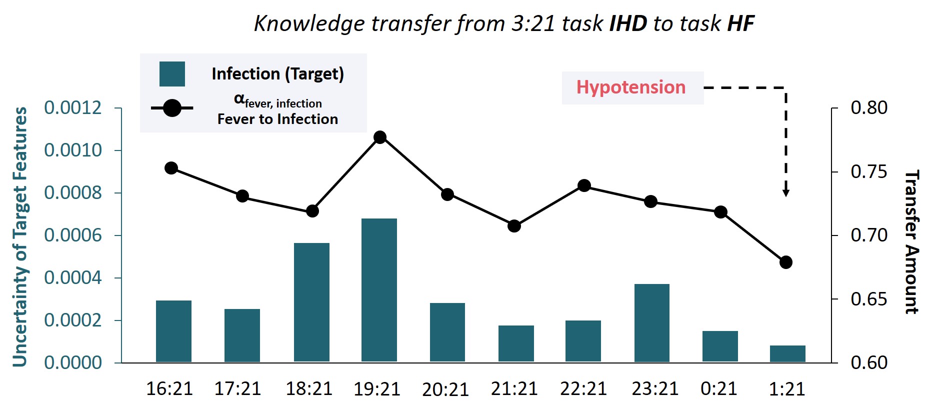
(a) KT from single timestep and Target Uncertainty

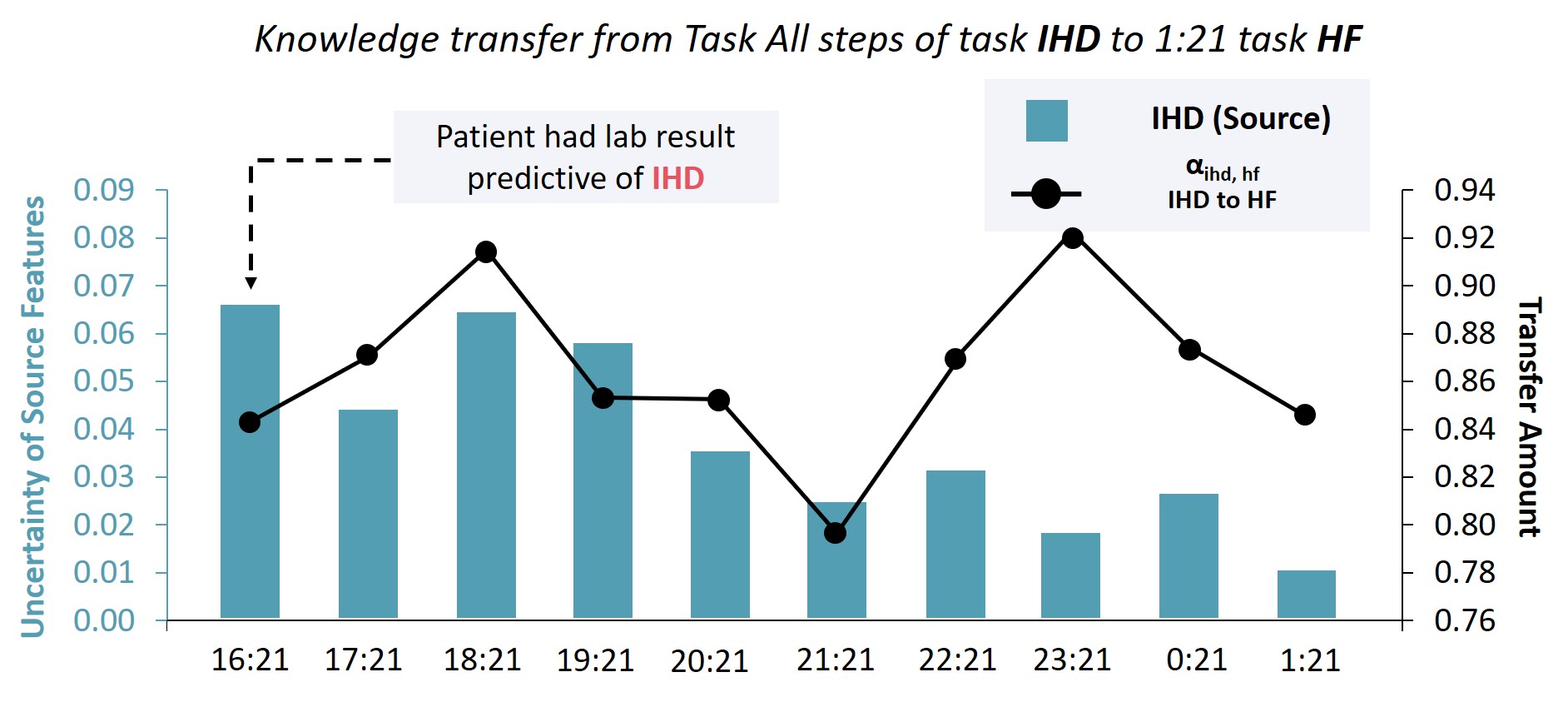
(b) KT to single timestep and Source Uncertainty

Figure 13: Uncertainty and Knowledge Transfer(KT) : Example case of MIMIC III - Heart Failure dataset where the changes in the amount of uncertainty at certain timesteps are correlated with clinical events. We denote the timesteps with noticeable changes in uncertainty and knowledge transfer with blue boxes.

MIMIC-III Respiratory Failure

With the help of a physician, we further analyze how generated transfer weights and uncertainties between tasks can be used to track changes in the relationships between clinical events and (see Figure 14). We first consider an example record of a patient from the MIMIC-III Respiratory Failure(RF) dataset who was found to be in hypercarbic(high arterial $CO_{2}$ pressure (high $P_{a}CO_{2}$, hypercapnia)) respiratory failure. Figure 14(a) shows the amount of knowledge transfer from task Hypoxia and Hypercapnia at $5:00AM$ to all later timesteps of task RF. As patient experience hypoxia (low arterial $O_{2}$ pressure (low $P_{a}O_{2}$)) during 12 ($19:00$) to 17 ($23:00$ AM) hours of admission, the uncertainty of hypoxia (blue bar chart of Figure 14(a)) drops accordingly, and knowledge transfers from task Hypoxia to task RF (dark blue line graph in Figure 14(a)). As patient was hypercarbic on admission, uncertainty of the task Hypercapnia kept its low value (dark blue bar chart in Figure 14(a)) and knowledge transfer to task RF is constantly high (dark blue line chart in Figure 14(a)). After $23:00$, $P_{a}O_{2}$ increases back to knowledge transfer drops as the uncertainty of task hypoxia increases. Change in learned knowledge graph can also be used for treatment planning, such as deciding whether the patient needs prompt oxygen infusion or not. Later in timestep $20$ ($01:00$), the $O_{2}$ Saturation of this patient drops to $78$ (see Figure  14(b)) and uncertainty of task $S_{a}O_{2}$ drops accordingly as a result of respiratory failure (dark green bar chart in Figure  14(b)). As the target uncertainty drops, knowledge transfer drops accordingly. After treatment $S_{a}O_{2}$ increases up to $94$ and then drops again to $83$ in timestep $23$ ($4:00$), where knowledge transfer from source task RF increases and drops accordingly in Figure  14(b) (black line).

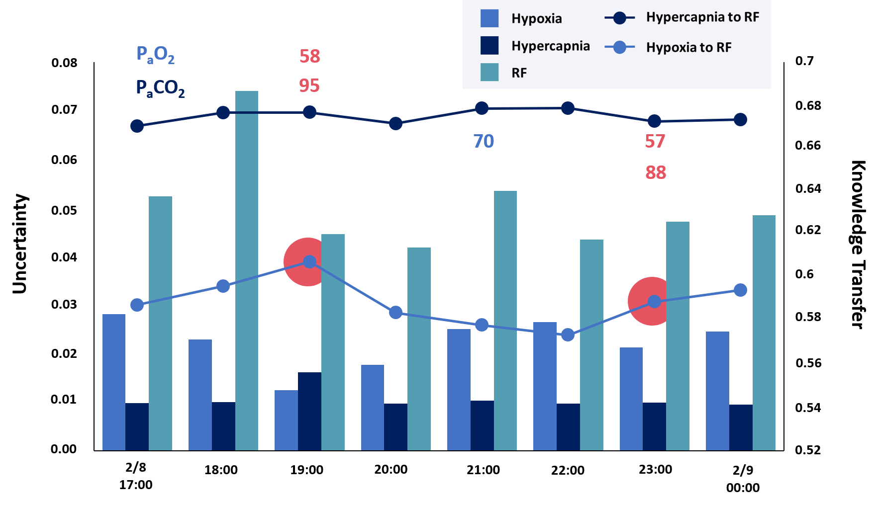
(a) KT from Hypoxemia, Hypercapnia to RF

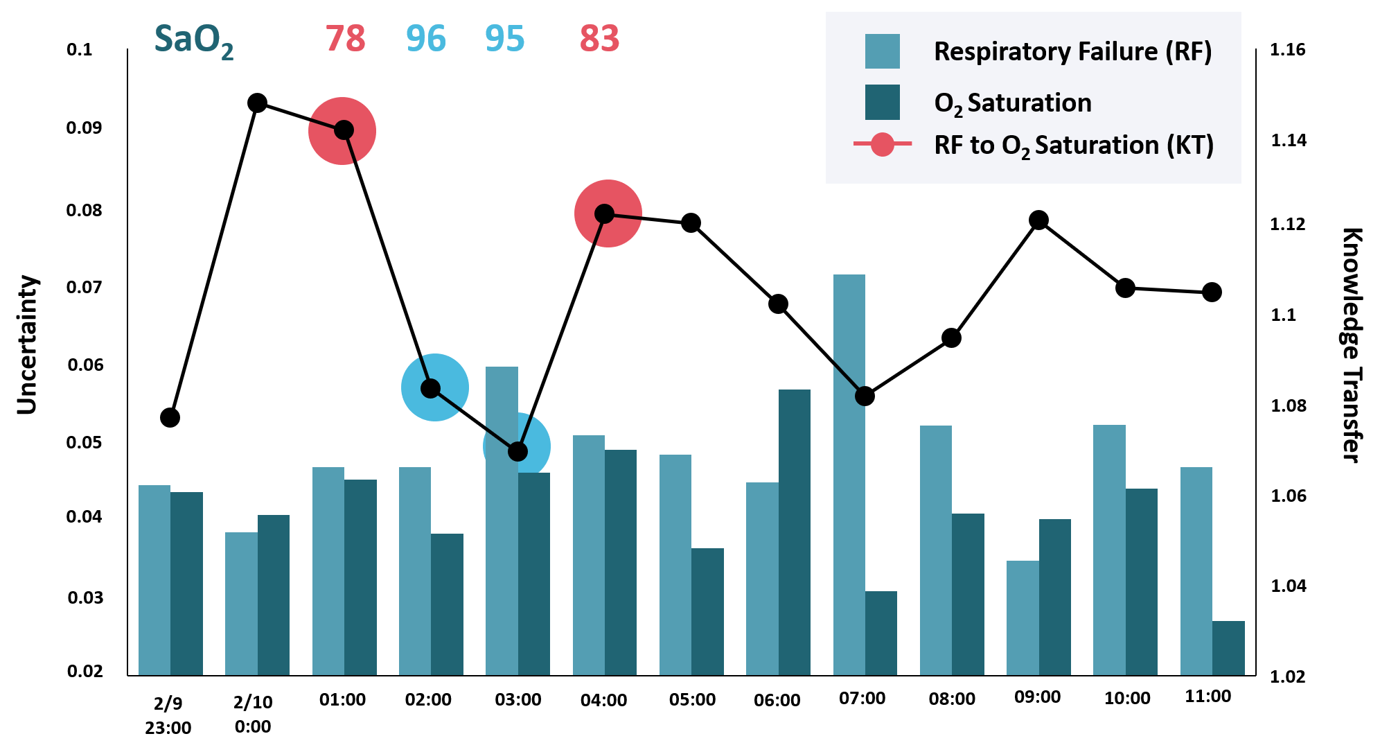
(b) KT from RF to $S_{a}O_{2}$

Figure 14: Visualizations of the amount of uncertainty and normalized knowledge transfer for example cases where the changes in the amount of uncertainty at certain timesteps are correlated with clinical events. We denote the timesteps with noticeable changes in uncertainty and knowledge transfer with Red(fatal clinical condition predictive of target task), Blue(improved patient condition)

Broader Impact

In this paper, we present Temporal Probabilistic Asymmetric Multi-Task Learning (TPAMTL) model, which is appropriate for various multi-task time-series predictions with strong performance while preventing negative transfer. Our model is especially applicable to safety-critical clinical risk predictions, as it provides a reliable explanation of its final prediction on each task at each timestep. Here in this section, we introduce the clinical and social impact of our model.

Safe and Reliable AI for Clinical risk prediction

With the actual knowledge transfer graph plotted with uncertainty obtained at each timestep, healthcare professionals could interpret the behaviors of model according to actual clinical events in multiple clinical risk prediction tasks (Figure 4, Supplementary Figure 11, 12, 13). By checking the knowledge transfer graph and the amount of uncertainty measured for each task at each timestep, our model can provide medical professionals with a better explanation of the underlying model behavior. Based on this explanation, medical experts can have a clue on the direction of knowledge transfer, or say interaction, between tasks, which might help them decide future action: whether to consult other departments for medical opinion, to run a further test to confirm the predicted event, or to come up with better treatment plan. This interpretability of our model will be useful in building a safe time-series analysis system for large-scale settings where both the number of time-series data instances and timestep are extremely large, such that manual analysis is impractical.

Monitoring clinical events of critical ill patient

Due to the unprecedented pandemic outbreak of coronavirus infection (COVID-19) this year, hospitals worldwide are suffering from the lack of healthcare professionals and facilities to monitor and care for patients [36]. In this era of difficulty, machine learning models can aid the diagnosis [20, 34], drug repositioning [29], predicting patient condition, and epidemiological trends of disease [23]. One example of this large-scale setting would be the situation to monitor COVID-19, where the number of newly diagnosed patients is increasing daily [25], and there is a need to follow-up on multiple outcomes (pneumonia [35], cardiac disease related to myocardial injury [8], etc.) of this infection, also in relation to underlying disease each patient had, where no pathophysiological and case information is available. In this situation when the number of patients exceeds the capacity of the healthcare system, a prediction model with a better capacity of handling large-scale data can help reduce the burden of healthcare staff. Not only the acute clinical conditions (e.g., infection), but also the chronic clinical conditions, such as conditions and abnormalities related to heart failure (Task MIMIC-III Heart Failure) or respiratory failure (Task MIMIC-III Respiratory Failure), can be monitored with our model, as our model provides long-term prediction without degeneration of performance, still providing reliable information.

Table 11: Feature information of MIMIC III - Infection dataset

Features	Item-ID	Name of Item
Age	NA	initime dob
Sex	NA	gender
	211	Heart Rate
Heart Rate	22045	Heart Rate
	51	Systolic Blood Pressure
	442	Systolic Blood Pressure
	455	Systolic Blood Pressure
	6701	Systolic Blood Pressure
	220179	Systolic Blood Pressure
Systolic Blood Pressure	220050	Systolic Blood Pressure
	8368	Diastolic Blood Pressure
	8440	Diastolic Blood Pressure
	8441	Diastolic Blood Pressure
	8555	Diastolic Blood Pressure
	220051	Diastolic Blood Pressure
Diastolic Blood Pressure	220180	Diastolic Blood Pressure
	223900	GCS-Verbal Response
	223901	GCS-Motor Response
Glasgow Coma Scale	220739	GCS-Eye Opening
	225433	Chest Tube Placed
	5456	Chest Tube
	225445	Paracentesis
	225446	PEG Insertion
	225399	Lumbar Puncture
	5939	Lumbar drain
	225469	OR Received
	225442	Liver Biopsy
	224264	PICC Line
	224560	PA Catheter
	225430	Cardiac Cath
	225315	Tunneled (Hickman) Line
	226475	Intraventricular Drain Inserted
Invasive procedures	5889	Bladder cath
	225434	Colonoscopy
	225439	Endoscopy
Endoscopic Procedure	227550	ERCP
	224385	Intubation
	225448	Percutaneous Tracheostomy
	225468	Unplanned Extubation (patient-initiated)
	225477	Unplanned Extubation (non-patient initiated)
	226237	Open Tracheostomy
Intubation / Unplanned Extubation	225792	Invasive Ventilation
	772	Albumin (>3.2)
	1521	Albumin
	227456	Albumin
	3727	Albumin (3.9-4.8)
	226981	Albumin_ApacheIV
Albumin	226982	AlbuminScore_ApacheIV
	220650	Total Protein(6.5-8)
	849	Total Protein(6.5-8)
	3807	Total Protein
	1539	Total Protein(6.5-8)
Total Protein	220650	Total Protein(6.5-8)

Table 12: Feature information of MIMIC III - Infection dataset: continued

Features	Item-ID	Name of Item
	225441	Hemodialysis
	225805	Peritoneal Dialysis
	226477	Temporary Pacemaker Wires Inserted
	224270	Dialysis Catheter
	225802	Dialysis - CRRT
Dialysis	225805	Peritoneal Dialysis
	4929	Prednisolone
	7772	Predisolone
	6753	Prednisilone gtts
	6111	prednisone
	8309	prednisolone gtts
	5003	prednisolone
	1878	methylprednisolone
	2656	SOLUMEDROL MG/KG/HR
	2657	SOLUMEDROL CC/H
	2629	SOLUMEDROL DRIP
	2983	solumedrol mg/hr
	7425	Solu-medrol mg/hr
	6323	solumedol
	7592	Solumedrol cc/h
	30069	Solumedrol
	2959	Solumedrolmg/kg/hr
	1878	methylprednisolone
	5395	Beclamethasone
	4542	Tobradex
	5612	Dexamethasone gtts
	3463	Hydrocortisone
Intravenous Steroid	8070	dexamethasone gtts

Table 13: Disease information of MIMIC III - Heart Failure dataset

Task Name	ICD9 Disease Code
	412, 4110, 4148, 4149, 41000, 41001, 41002, 41010, 41011, 41012,
	41020, 41021, 41022, 41030, 41031, 41032, 41040, 41041, 41042, 41050,
	41051, 41052, 41060, 41061, 41062, 41070, 41071, 41072, 41080, 41082,
Ischemic Heart Disease (IHD)	41090, 41091, 41092, 41181, 41189, 41406, 41407
	3940, 3942, 3949, 3952, 3960, 3961, 3962, 3963, 3968, 3969,
Valvular Heart Disease (VHD)	3970, 3971, 4240, 4241, 4242, 4243, V422, V433
	4280, 4281, 39831, 40201, 40211, 40291, 40401, 40403, 40411, 40413,
	40491, 40493, 42820, 42821, 42822, 42823, 42830, 42831, 42832, 42833,
Heart Failure (HF)	42840, 42841, 42842, 42843
Mortality	NA

Table 14: Feature information of MIMIC III - Heart Failure dataset

Features	Item-ID	Name of Item
Age	NA	initime dob
Sex	NA	gender
	211	Heart Rate
Heart Rate	22045	Heart Rate
	618	Respiratory Rate
	619	Respiratory Rate
	220210	Respiratory Rate
	224688	Respiratory Rate
	224689	Respiratory Rate
Respiratory Rate	224690	Respiratory Rate
	51	Systolic Blood Pressure
	442	Systolic Blood Pressure
	455	Systolic Blood Pressure
	6701	Systolic Blood Pressure
	220179	Systolic Blood Pressure
Systolic Blood Pressure	220050	Systolic Blood Pressure
	8368	Diastolic Blood Pressure
	8440	Diastolic Blood Pressure
	8441	Diastolic Blood Pressure
	8555	Diastolic Blood Pressure
	220051	Diastolic Blood Pressure
Diastolic Blood Pressure	220180	Diastolic Blood Pressure
	676	Body Temperature
	677	Body Temperature
	8537	Body Temperature
	223762	Body Temperature
Body Temperature	226329	Body Temperature
	189	Fi$O_{2}$
	190	Fi$O_{2}$
	2981	Fi$O_{2}$
	3420	Fi$O_{2}$
	3422	Fi$O_{2}$
Fraction of inspired oxygen (Fi$O_{2}$)	223835	Fi$O_{2}$
	823	$S_{v}O_{2}$
	2396	$S_{v}O_{2}$
	2398	$S_{v}O_{2}$
	2574	$S_{v}O_{2}$
	2842	$S_{v}O_{2}$
	2933	$S_{v}O_{2}$
	2955	$S_{v}O_{2}$
	3776	$S_{v}O_{2}$
	5636	$S_{v}O_{2}$
	6024	$S_{v}O_{2}$
	7260	$S_{v}O_{2}$
	7063	$S_{v}O_{2}$
	7293	$S_{v}O_{2}$
	226541	$S_{v}O_{2}$
	227685	$S_{v}O_{2}$
	225674	$S_{v}O_{2}$
Mixed venous Oxygen Saturation ($S_{v}O_{2}$)	227686	$S_{v}O_{2}$
	834	$S_{a}O_{2}$
	3288	$S_{a}O_{2}$
	8498	$S_{a}O_{2}$
Oxygen Saturation of arterial blood ($S_{a}O_{2}$)	220227	$S_{a}O_{2}$
	7294	BNP
	227446	BNP
Brain Natriuretic Peptide (BNP)	225622	BNP
Ejection Fraction (EF)	227008	EF
Glasgow Coma Scale (GCS) - Verbal Response	223900	GCS-Verbal Response
Glasgow Coma Scale (GCS) - Motor Response	223901	GCS-Motor Response
Glasgow Coma Scale (GCS) - Eye Opening	220739	GCS-Eye Opening

Table 15: Disease information of MIMIC III - Respiratory Failure dataset

Task Name (Clinical Condition)	Item-ID	Name of Item
	779	Arterial $P_{a}O_{2}$
	3785	$P_{a}O_{2}$ (ABG’s)
	3837	$P_{a}O_{2}$ (ABG’s)
	3838	$P_{a}O_{2}$ (other)
	4203	$P_{a}O_{2}$ (cap)
Hypoxia ($P_{a}O_{2}<60mmHg$)	220224	$P_{a}O_{2}$ (Arterial $O_{2}$ Pressure)
	778	Arterial $P_{a}CO_{2}$
	3784	$P_{a}CO_{2}$ (ABG’s)
	3835	$P_{a}CO_{2}$
	3836	$P_{a}CO_{2}$ (other)
	4201	$P_{a}CO_{2}$ (cap)
Hypercapnia (Hypercarbia, $P_{a}CO_{2}>50mmHg$)	220224	$P_{a}CO_{2}$ (Arterial $CO_{2}$ Pressure)
VQ Mismatch	26	Alveolar-arterial oxygen gradient ($A_{a}DO_{2}$)
	780	Arterial pH
	1126	Art.pH
	3839	ph (other)
	4202	ph (cap)
Acidosis (Arterial $pH<7.35$)	4753	ph (Art)
	51881	Acute Respiratory Failure (ARF)
	51883	Chronic Respiratory Failure (CRF)
Respiratory Failure (RF)	51884	ARF, CRF
	834	$S_{a}O_{2}$
	3288	$O_{2}$ sat [Pre]
	4833	$S_{a}O_{2}$ (post)
	8498	$O_{2}$ sat [Post]
Cyanosis: Patient requiring $O_{2}$ infusion ($O_{2}$ Saturation($S_{a}O_{2}$) $<94$)	$220227$	Arterial $O_{2}$ Saturation
Mortality	NA

Table 16: Feature information of MIMIC III - Respiratory Failure dataset

Features	Item-ID	Name of Item
Age	NA	initime dob
Sex	NA	gender
	211	Heart Rate
Heart Rate	22045	Heart Rate
	618	Respiratory Rate
	619	Respiratory Rate
	220210	Respiratory Rate
	224688	Respiratory Rate
	224689	Respiratory Rate
Respiratory Rate	224690	Respiratory Rate
	51	Systolic Blood Pressure
	442	Systolic Blood Pressure
	455	Systolic Blood Pressure
	6701	Systolic Blood Pressure
	220179	Systolic Blood Pressure
Systolic Blood Pressure	220050	Systolic Blood Pressure
	8368	Diastolic Blood Pressure
	8440	Diastolic Blood Pressure
	8441	Diastolic Blood Pressure
	8555	Diastolic Blood Pressure
	220051	Diastolic Blood Pressure
Diastolic Blood Pressure	220180	Diastolic Blood Pressure
	676	Body Temperature
	677	Body Temperature
	8537	Body Temperature
	223762	Body Temperature
Body Temperature	226329	Body Temperature
Bicarbonate ($HCO_{3}^{-}$)	812	$HCO_{3}^{-}$
Base Excess (BE)	812	BE
	189	Fi$O_{2}$
	190	Fi$O_{2}$
	2981	Fi$O_{2}$
	3420	Fi$O_{2}$
	3422	Fi$O_{2}$
Fraction of inspired oxygen (Fi$O_{2}$)	223835	Fi$O_{2}$
	823	$S_{v}O_{2}$
	2396	$S_{v}O_{2}$
	2398	$S_{v}O_{2}$
	2574	$S_{v}O_{2}$
	2842	$S_{v}O_{2}$
	2933	$S_{v}O_{2}$
	2955	$S_{v}O_{2}$
	3776	$S_{v}O_{2}$
	5636	$S_{v}O_{2}$
	6024	$S_{v}O_{2}$
	7260	$S_{v}O_{2}$
	7063	$S_{v}O_{2}$
	7293	$S_{v}O_{2}$
	226541	$S_{v}O_{2}$
	227685	$S_{v}O_{2}$
	225674	$S_{v}O_{2}$
Mixed venous Oxygen Saturation ($S_{v}O_{2}$)	227686	$S_{v}O_{2}$
Partial Pressure of Oxygen in the Alveoli ($P_{A}O_{2}$)	490	$P_{A}O_{2}$
Arterial Oxygen Content ($C_{a}O_{2}$)	114	$C_{a}O_{2}$
Venous Oxygen Content ($C_{v}O_{2}$)	143	$C_{v}O_{2}$
	1390	$DO_{2}$
	1391	$DO_{2}$
Delivered Oxygen ($DO_{2}$)	2740	$DO_{2}$
	504	$PCWP$
Pulmonary Capillary Wedge Pressure (PCWP)	223771	PCWP
Positive End-Expiratory Pressure (PEEP)	505	PEEP

Table 17: Feature information of MIMIC III - Respiratory Failure dataset: continued

Features	Item-ID	Name of Item
	814	$Hb$
Hemoglobin ($Hb$)	220228	$Hb$
Red Blood Cell (RBC)	223901	RBC
	861	WBC
	1127	WBC
	1542	WBC
White Blood Cell (WBC)	220546	WBC
	828	Platelet
	30006	Platelet
Platelet	225170	Platelet
	1162	BUN
	5876	BUN
Blood Urine Nitrogen (BUN)	225624	BUN
	1525	Creatinine
Creatinine	220615	Creatinine
	7294	BNP
	227446	BNP
Brain Natriuretic Peptide (BNP)	225622	BNP
Ejection Fraction (EF)	227008	EF
Glasgow Coma Scale (GCS) - Verbal Response	223900	GCS-Verbal Response
Glasgow Coma Scale (GCS) - Motor Response	223901	GCS-Motor Response
Glasgow Coma Scale (GCS) - Eye Opening	220739	GCS-Eye Opening

References

- Argyriou, Evgeniou, and Pontil [2008] Argyriou, A.; Evgeniou, T.; and Pontil, M. 2008. Convex multi-task feature learning. Machine Learning 73(3): 243–272.
- Caruana [1997] Caruana, R. 1997. Multitask learning. Machine learning 28(1): 41–75.
- Che et al. [2018] Che, Z.; Purushotham, S.; Cho, K.; Sontag, D.; and Liu, Y. 2018. Recurrent neural networks for multivariate time series with missing values. Scientific reports 8(1): 1–12.
- Choi et al. [2016] Choi, E.; Bahadori, M. T.; Sun, J.; Kulas, J.; Schuetz, A.; and Stewart, W. 2016. Retain: An interpretable predictive model for healthcare using reverse time attention mechanism. In Advances in Neural Information Processing Systems, 3504–3512.
- Citi and Barbieri [2012] Citi, L.; and Barbieri, R. 2012. PhysioNet 2012 Challenge: Predicting mortality of ICU patients using a cascaded SVM-GLM paradigm. In 2012 Computing in Cardiology, 257–260. IEEE.
- Duong et al. [2015] Duong, L.; Cohn, T.; Bird, S.; and Cook, P. 2015. Low resource dependency parsing: Cross-lingual parameter sharing in a neural network parser. In Proceedings of the 53rd Annual Meeting of the Association for Computational Linguistics and the 7th International Joint Conference on Natural Language Processing (Volume 2: Short Papers), volume 2, 845–850.
- Gal and Ghahramani [2016] Gal, Y.; and Ghahramani, Z. 2016. Dropout as a bayesian approximation: Representing model uncertainty in deep learning. In international conference on machine learning, 1050–1059.
- Guo et al. [2020] Guo, T.; Fan, Y.; Chen, M.; Wu, X.; Zhang, L.; He, T.; Wang, H.; Wan, J.; Wang, X.; and Lu, Z. 2020. Cardiovascular implications of fatal outcomes of patients with coronavirus disease 2019 (COVID-19). JAMA cardiology .
- Harutyunyan et al. [2019] Harutyunyan, H.; Khachatrian, H.; Kale, D. C.; Ver Steeg, G.; and Galstyan, A. 2019. Multitask learning and benchmarking with clinical time series data. Scientific data 6(1): 1–18.
- Heo et al. [2018] Heo, J.; Lee, H. B.; Kim, S.; Lee, J.; Kim, K. J.; Yang, E.; and Hwang, S. J. 2018. Uncertainty-aware attention for reliable interpretation and prediction. In Advances in Neural Information Processing Systems, 909–918.
- Johnson, Pollard, and Mark [2017] Johnson, A. E.; Pollard, T. J.; and Mark, R. G. 2017. Reproducibility in critical care: a mortality prediction case study. In Machine Learning for Healthcare Conference, 361–376.
- Johnson et al. [2016] Johnson, A. E.; Pollard, T. J.; Shen, L.; Li-wei, H. L.; Feng, M.; Ghassemi, M.; Moody, B.; Szolovits, P.; Celi, L. A.; and Mark, R. G. 2016. MIMIC-III, a freely accessible critical care database. Scientific data 3: 160035.
- Kang, Grauman, and Sha [2011] Kang, Z.; Grauman, K.; and Sha, F. 2011. Learning with Whom to Share in Multi-task Feature Learning. In ICML, volume 2, 4.
- Kendall and Gal [2017] Kendall, A.; and Gal, Y. 2017. What uncertainties do we need in bayesian deep learning for computer vision? In Advances in neural information processing systems, 5574–5584.
- Kendall, Gal, and Cipolla [2018] Kendall, A.; Gal, Y.; and Cipolla, R. 2018. Multi-task learning using uncertainty to weigh losses for scene geometry and semantics. In Proceedings of the IEEE Conference on Computer Vision and Pattern Recognition, 7482–7491.
- Kumar and Daume III [2012] Kumar, A.; and Daume III, H. 2012. Learning task grouping and overlap in multi-task learning. arXiv preprint arXiv:1206.6417 .
- LeCun and Cortes [2010] LeCun, Y.; and Cortes, C. 2010. MNIST handwritten digit database. http://yann.lecun.com/exdb/mnist/. URL http://yann.lecun.com/exdb/mnist/.
- Lee, Yang, and Hwang [2016] Lee, G.; Yang, E.; and Hwang, S. 2016. Asymmetric multi-task learning based on task relatedness and loss. In International Conference on Machine Learning, 230–238.
- Lee, Yang, and Hwang [2017] Lee, H. B.; Yang, E.; and Hwang, S. J. 2017. Deep Asymmetric Multi-task Feature Learning. arXiv preprint arXiv:1708.00260 .
- Li et al. [2020] Li, L.; Qin, L.; Xu, Z.; Yin, Y.; Wang, X.; Kong, B.; Bai, J.; Lu, Y.; Fang, Z.; Song, Q.; et al. 2020. Artificial intelligence distinguishes COVID-19 from community acquired pneumonia on chest CT. Radiology 200905.
- Ma et al. [2020] Ma, L.; Gao, J.; Wang, Y.; Zhang, C.; Wang, J.; Ruan, W.; Tang, W.; Gao, X.; and Ma, X. 2020. AdaCare: Explainable Clinical Health Status Representation Learning via Scale-Adaptive Feature Extraction and Recalibration. In Proceedings of the AAAI Conference on Artificial Intelligence, volume 34, 825–832.
- Maurer, Pontil, and Romera-Paredes [2013] Maurer, A.; Pontil, M.; and Romera-Paredes, B. 2013. Sparse coding for multitask and transfer learning. In International conference on machine learning, 343–351.
- McCall [2020] McCall, B. 2020. COVID-19 and artificial intelligence: protecting health-care workers and curbing the spread. The Lancet Digital Health 2(4): e166–e167.
- Misra et al. [2016] Misra, I.; Shrivastava, A.; Gupta, A.; and Hebert, M. 2016. Cross-stitch networks for multi-task learning. In Proceedings of the IEEE Conference on Computer Vision and Pattern Recognition, 3994–4003.
- Novel et al. [2020] Novel, C. P. E. R. E.; et al. 2020. The epidemiological characteristics of an outbreak of 2019 novel coronavirus diseases (COVID-19) in China. Zhonghua liu xing bing xue za zhi= Zhonghua liuxingbingxue zazhi 41(2): 145.
- Pirracchio [2016] Pirracchio, R. 2016. Mortality prediction in the icu based on mimic-ii results from the super icu learner algorithm (sicula) project. In Secondary Analysis of Electronic Health Records, 295–313. Springer.
- Purushotham et al. [2017] Purushotham, S.; Meng, C.; Che, Z.; and Liu, Y. 2017. Benchmark of deep learning models on large healthcare mimic datasets. arXiv preprint arXiv:1710.08531 .
- Reichlin et al. [2009] Reichlin, T.; Hochholzer, W.; Bassetti, S.; Steuer, S.; Stelzig, C.; Hartwiger, S.; Biedert, S.; Schaub, N.; Buerge, C.; Potocki, M.; et al. 2009. Early diagnosis of myocardial infarction with sensitive cardiac troponin assays. New England Journal of Medicine 361(9): 858–867.
- Richardson et al. [2020] Richardson, P.; Griffin, I.; Tucker, C.; Smith, D.; Oechsle, O.; Phelan, A.; and Stebbing, J. 2020. Baricitinib as potential treatment for 2019-nCoV acute respiratory disease. Lancet (London, England) 395(10223): e30.
- Ruder et al. [2017] Ruder, S.; Bingel, J.; Augenstein, I.; and Søgaard, A. 2017. Learning what to share between loosely related tasks. ArXiv .
- Song et al. [2018] Song, H.; Rajan, D.; Thiagarajan, J. J.; and Spanias, A. 2018. Attend and diagnose: Clinical time series analysis using attention models. In Thirty-Second AAAI Conference on Artificial Intelligence.
- UdeM [2014] UdeM. 2014. Variations on the MNIST Digits. URL https://sites.google.com/a/lisa.iro.umontreal.ca/public˙static˙twiki/variations-on-the-mnist-digits.
- Vaswani et al. [2017] Vaswani, A.; Shazeer, N.; Parmar, N.; Uszkoreit, J.; Jones, L.; Gomez, A. N.; Kaiser, Ł.; and Polosukhin, I. 2017. Attention is all you need. In Advances in neural information processing systems, 5998–6008.
- Wang and Wong [2020] Wang, L.; and Wong, A. 2020. COVID-Net: A tailored deep convolutional neural network design for detection of COVID-19 cases from chest radiography images. arXiv arXiv–2003.
- Woo et al. [2004] Woo, P. C.; Lau, S. K.; Tsoi, H.-w.; Chan, K.-h.; Wong, B. H.; Che, X.-y.; Tam, V. K.; Tam, S. C.; Cheng, V. C.; Hung, I. F.; et al. 2004. Relative rates of non-pneumonic SARS coronavirus infection and SARS coronavirus pneumonia. The Lancet 363(9412): 841–845.
- Xie et al. [2020] Xie, J.; Tong, Z.; Guan, X.; Du, B.; Qiu, H.; and Slutsky, A. S. 2020. Critical care crisis and some recommendations during the COVID-19 epidemic in China. Intensive care medicine 1–4.
- Yang and Hospedales [2016a] Yang, Y.; and Hospedales, T. 2016a. Deep multi-task representation learning: A tensor factorisation approach. arXiv preprint arXiv:1605.06391 .
- Yang and Hospedales [2016b] Yang, Y.; and Hospedales, T. M. 2016b. Trace norm regularised deep multi-task learning. arXiv preprint arXiv:1606.04038 .