Subcompartmentalization of polyampholyte species in organelle-like condensates is promoted by charge pattern mismatch and strong excluded-volume interaction

Abstract

Polyampholyte field theory and explicit-chain molecular dynamics models of sequence-specific phase separation of a system with two intrinsically disordered protein (IDP) species indicate consistently that a substantial polymer excluded volume and a significant mismatch of the IDP sequence charge patterns can act in concert, but not in isolation, to demix the two IDP species upon condensation. This finding reveals an energetic-geometric interplay in a stochastic, “fuzzy” molecular recognition mechanism that may facilitate subcompartmentalization of membraneless organelles.

I Introduction

Liquid-liquid phase separation (LLPS) Brangwynne et al. (2009); Li et al. (2012); Kato et al. (2012); Hyman et al. (2014); Nott et al. (2015) in biomolecular condensates Banani et al. (2017) has garnered intense interest in diverse areas of biomedicine, biophysics, and polymer physics Alberti (2017). LLPS plays a central role in the assembly of droplet-like cellular compartments—coexisting with a more dilute milieu and sometimes referred to as membraneless organelles—that act as hubs for biochemical processes. Examples include nucleoli, P-bodies, stress granules, and cajal bodies. Serving critical organismal functions, their misregulation can cause disease Molliex et al. (2015); Li et al. (2018).

Biomolecular LLPS often involves intrinsically disordered proteins (IDPs) and nucleic acids participating in multivalent interactions Chen et al. (2015); Brangwynne et al. (2015). Recent theories and computational studies have begun to shed light on how LLPSs of IDPs are governed by their amino acid sequences. These efforts include analytical theory Lin et al. (2016); Chang et al. (2017); Lin et al. (2020); Amin et al. (2020), explicit-chain lattice Feric et al. (2016); Das et al. (2018a); Choi et al. (2019) and continuum molecular dynamics (MD) Dignon et al. (2018a); Das et al. (2018b); Statt et al. (2020); Hazra and Levy (2020); Das et al. (2020); Hazra and Levy (2021) simulations, and field-theoretic simulation (FTS) Lin et al. (2019); McCarty et al. (2019); Danielsen et al. (2019a), investigations of the relationship between LLPS propensity and single/double-chain properties Lin and Chan (2017); Dignon et al. (2018b); Amin et al. (2020) as well as crystals and filaments formation Robichaud et al. (2019), and studies of the peculiar temperature Cinar et al. (2019a); Dignon et al. (2019a) and pressure Cinar et al. (2019a, 2020) dependence of biomolecular LLPS as well as finite-size scaling in droplet formation Nilsson and Irbäck (2020). Reviews of the emerging theoretical perspectives are available in Refs. (35; 36; 37; 38; 39).

IDPs are enriched in charged and polar residues Uversky (2002) and multivalent electrostatics is an important driving force—among others Vernon et al. (2018)—for LLPS. One consistent finding from theory Lin et al. (2016), chain simulation Das et al. (2018a, b) and FTS McCarty et al. (2019); Danielsen et al. (2019a) is that the LLPS propensity of a polyampholyte depends on its sequence charge pattern, which may be quantified by an intuitive blockiness $\kappa$ measure Das and Pappu (2013) or an analytic “sequence charge decoration” (SCD) parameter Sawle and Ghosh (2015) that correlates with single-chain properties Das and Pappu (2013); Sawle and Ghosh (2015); Huihui and Ghosh (2020).

While simple laboratory systems may contain only one IDP type (species), many types of IDPs interact in the cell to compartmentalize into a variety of condensates. In some cases, LLPS-mediated organization of intracellular space goes a step further by subcompartmentalization Thiry and Lafontaine (2005). Well-known examples include the nucleolus comprising of at least three subcompartments enriched with distinct sets of proteins A and Weber (2019); Feric et al. (2016) and stress granules with a dense core surrounded by a liquid-like outer shell Jain et al. (2016). These phenomena raise intriguing physics questions as to the nature of the sequence-specific interactions that drive a subset of IDPs in a condensate to coalesce among themselves while excluding other types of IDPs.

Insights into formation of subcompartments Feric et al. (2016); Harmon et al. (2018); Mazarakos and Zhou (2021) and general principles of many-component phase behaviors Jacobs and Frenkel (2017) have been gained from models with energies assigned to favor or disfavor interactions between different solute components. On a more fundamental level, a random phase approximation (RPA) Ermoshkin and Olvera de la Cruz (2003); Lin et al. (2016) model of two polyampholytic IDP species suggested that sequence-specific molecular recognition can arise from elementary electrostatic interactions in a stochastic, “fuzzy” manner, in that the IDP species in the LLPS condensed phase are predicted to demix when their sequence charge patterns are significantly different (large difference in their SCD values), but tend to be miscible when their SCD values are similar Lin et al. (2017a). This trend is also rationalized by a recent analysis of second virial coefficients Amin et al. (2020).

Table 1: Hamiltonians used in this work; $\beta=1/k_{\mathrm{B}}T$, where $k_{\mathrm{B}}$ is Boltzmann’s constant and $T$ is absolute temperature.

	$\hat{H}_{0}$	$\hat{H}_{1}$	$\hat{H}_{2}$
FTS:	$\frac{3}{2b^{2}\beta}$ $\sum\limits_{p,i,\alpha}|\bm{r}_{p,i,\alpha+1}-\bm{r}_{p,i,\alpha}|^{2}$	$\frac{v}{2\beta}$ $\int\mathrm{d}\bm{r}\int\mathrm{d}\bm{r}^{\prime}\hat{\rho}_{\mathrm{b}}(\bm{r})\delta(\bm{r}-\bm{r}^{\prime})\hat{\rho}_{\mathrm{b}}(\bm{r}^{\prime})$	$\Biggl{|}$ ${\frac{l_{\mathrm{B}}}{2\beta}}$ $\int\mathrm{d}\bm{r}\int\mathrm{d}\bm{r}^{\prime}$ $\frac{\hat{\rho}_{\mathrm{c}}(\bm{r})\hat{\rho}_{\mathrm{c}}(\bm{r}^{\prime})}{|\bm{r}-\bm{r}^{\prime}|}$
MD:	$\frac{K_{\mathrm{b}}}{2}$ $\sum\limits_{p,i,\alpha}(|\bm{r}_{p,i,\alpha+1}-\bm{r}_{p,i,\alpha}|-a_{0})^{2}$	$\frac{2\epsilon}{3}$ $\sum\limits_{\begin{subarray}{c}p,i,\alpha,\\ \neq q,j,\gamma\end{subarray}}$ $\hskip-5.69054pt\Bigl{[}\Bigl{(}$ $\frac{r_{0}}{|\bm{r}_{p,i,\alpha}-\bm{r}_{q,j,\gamma}|}$ $\Bigr{)}^{12}-\Bigl{(}$ $\frac{r_{0}}{|\bm{r}_{p,i,\alpha}-\bm{r}_{q,j,\gamma}|}$ $\Bigr{)}^{6}\Bigr{]}$	$\frac{l_{\mathrm{B}}}{2\beta}$ $\sum\limits_{\begin{subarray}{c}p,i,\alpha,\\ \neq q,j,\gamma\end{subarray}}$ $\frac{\sigma_{p,\alpha}\sigma_{q,\gamma}}{|\bm{r}_{p,i,\alpha}-\bm{r}_{q,j,\gamma}|}$

Aiming to better understand the physics of selective compartmentalization in membraneless organelles, a question that must be tackled is how sequence charge pattern and polymer excluded volume interplay in the mixing/demixing of condensed polyampholyte species. The question arises because excluded volume was not fully accounted for in RPA Lin et al. (2017a) but excluded volume is a known factor in LLPS Das et al. (2018b); McCarty et al. (2019) and other condensed-phase properties Adroher-Ben\́mathrm{missing}itez et al. (2017); Sorichetti et al. (2018). In the present work, we address this fundamental question by using FTS and MD to model polyampholytes with short-range excluded volume repulsion and long-range Coulomb interaction. By construction, FTS is more accurate than RPA in the field-theoretic context if discretization and finite-volume errors can be neglected, whereas MD is more suitable for chemically realistic interactions and its microscopic structural information is accessible. As shown below, both models indicate that while charge pattern mismatch is necessary for demixing of different polyampholyte species in the condensed phase, the degree of demixing is highly sensitive to excluded volume, underscoring that excluded volume is a critical organizing principle not only for folded protein structures Chan and Dill (1990); Maritan et al. (2000); Shakhnovich (2006) and disordered protein conformations Wallin and Chan (2005, 2006); Song et al. (2015) but also for biomolecular condensates.

II Model and Rationale

Here we study binary mixtures of two species of fully charged, overall neutral bead-spring polyampholytes $p,q$ differing only in their charge patterns, defined by the set of positions $\bm{r}_{p,i,\alpha}$ ($\bm{r}_{q,i,\alpha}$) of bead $\alpha$ on chain $i$ of type $p$ ($q$) with electric charges $\sigma_{p,\alpha}$ ($\sigma_{q,\alpha}$) for all $i$. The sequences considered (Fig. 1) are representative of the set of 50mer “sv sequences”, used extensively for modeling Sawle and Ghosh (2015); Lin and Chan (2017); Lin et al. (2017a); McCarty et al. (2019), that are listed in ascending $\kappa$ values from the least blocky, strictly alternating sv1 to the diblock sequence sv30 Das and Pappu (2013). As a first step in studying pertinent general principles, the simple, coarse-grained FTS and MD Hamiltonians $\hat{H}=\hat{H}_{0}+\hat{H}_{1}+\hat{H}_{2}$ in Table 1 are adopted without consideration of structural details and variations such as salt and pH dependence. While all of our model sequences have net zero charge and thus counterions are not needed to maintain overall neutrality of the system, experiments show that formation of biomolecular condensates is affected by salt and pH Alberti (2017); Brady et al. (2017). Recently, some of these effects are rationalized by an improved RPA formulation with renormalized Kuhn lengths for the LLPS of a single polyampholyte species Lin et al. (2020). The study of these effects should be extended to multiple IDP species in future efforts.

Following standard prescription, we have expressed $\hat{H}_{1}$ and $\hat{H}_{2}$ in terms of $\hat{\rho}_{\mathrm{b}}(\bm{r})=\sum_{p}\hat{\rho}_{\mathrm{b},p}(\bm{r})$, $\hat{\rho}_{\mathrm{c}}(\bm{r})=\sum_{p}\hat{\rho}_{\mathrm{c},p}(\bm{r})$ where $\hat{\rho}_{\mathrm{b},p}$ and $\hat{\rho}_{\mathrm{c},p}$ are, respectively, the microscopic bead (matter) and charge densities of polymer type $p$. The individual beads are modelled as normalized Gaussian distributions $\Gamma(\bm{r})=\exp(-\bm{r}^{2}/2a^{2})/(2\pi a^{2})^{3/2}$ centered at positions $\bm{r}_{p,i,\alpha}$ Riggleman et al. (2012); Wang (2010) such that $\hat{\rho}_{\mathrm{b},p}(\bm{r})=\sum_{i,\alpha}\,\,\Gamma(\bm{r}-\bm{r}_{p,i,\alpha})$, $\hat{\rho}_{\mathrm{c},p}(\bm{r})=\sum_{i,\alpha}\sigma_{p,\alpha}\Gamma(\bm{r}-\bm{r}_{p,i,\alpha})$. The chain connectivity term $\hat{H}_{0}$ takes the usual Gaussian form with Kuhn length $b$ for FTS and the harmonic form with force constant $K_{\mathrm{b}}$ for MD (thus $b$ corresponds to $a_{0}$); the excluded-volume term $\hat{H}_{1}$ entails a $\delta$-function with strength $v$ for FTS Edwards (1965); McCarty et al. (2019) and a Lennard-Jones (LJ) potential with well depth $\epsilon/3$ for MD Das et al. (2018b); whereas electrostatics is provided by $\hat{H}_{2}$ with Bjerrum length $l_{\mathrm{B}}=e^{2}/4\pi\epsilon_{0}\epsilon_{\rm r}k_{\rm B}T$, where $e$ is electronic charge, $\epsilon_{0}$ and $\epsilon_{\rm r}$ are, respectively, vacuum and relative permitttivity (larger $l_{\mathrm{B}}$ corresponds to stronger electrostatic interactions because of a smaller $\epsilon_{\rm r}$ and/or lower $T$).

The phase behavior and the mixing/demixing of fully charged, overall-neutral polyampholytic sv sequences Das and Pappu (2013) in the condensed phase are used here as an idealized system to investigate the electrostatic aspects of the driving forces for these phenomena. For real systems of biological or synthetically designed IDPs, other favorable interactions Brangwynne et al. (2015), including non-ionic and hydrophobic Cinar et al. (2019a); Dignon et al. (2019a); Krainer et al. (2021) and $\pi$-related Vernon et al. (2018); Das et al. (2020); Song et al. (2013) effects, can afford additional contributions to the stability of the condensed phase. Thus, the behavior of a model system simulated here at a given model temperature (a given $l_{\mathrm{B}}$) may correspond to that of a system of IDPs with similar electrostatic but additional favorable physical interactions at a higher experimental temperature (shorter $l_{\mathrm{B}}$). Bearing this in mind, we choose $l_{\mathrm{B}}=5b$ to obtain many of the FTS results presented below in order to ensure that the model sequence with the lowest LLPS propensity, namely sv1, would phase separate, because we are interested primarily in the mixing/demixing of different IDP species in the condensed phase. In other words, $l_{\mathrm{B}}=5b$ is lower than the upper critical solution temperatures (UCST) of all the sequences we consider. If we take $T=298.15$ K as room temperature and $b$ $=$ C_α–C_α virtual bond length $=$ $3.8$ Å, $l_{\mathrm{B}}=5b$ corresponds to a relative permittivity $\epsilon_{\rm r}\approx 30$ for the solvent plus IDP environment. While $l_{\mathrm{B}}=5b$ is larger than $l_{\mathrm{B}}\approx 1.8b\approx 7$Å if the $\epsilon_{\rm r}\approx 80$ for bulk water is assumed, it is instructive to note that the dielectric environment of the IDP condensed phase likely entails a smaller effective $\epsilon_{\rm r}$ than that of bulk water Das et al. (2020); Wessén et al. (2021), and that uniform relative permittivities with $\epsilon_{\rm r}$ values of $\approx 30$–$60$ have been used recently to match theoretical predictions with experimental LLPS data Nott et al. (2015); Lin et al. (2016, 2017b).

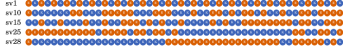
Figure 1: Polyampholytes studied in this work. Blue/red beads of “K”s (lysines)/“E”s (glutamic acids) carry $\pm 1$ protonic charges. The sv labels are those of Ref. (42).

III Field theoretic simulations (FTS)

The basic strategy of field-based approaches is to trade the explicit bead positions $\{\bm{r}_{p,i,\alpha}\}$ in favor of a set of interacting fields as the microscopic degrees of freedom (the mathematical procedure to achieve this is outlined below). The resulting statistical field theory contains the same thermodynamic information, and therefore thermal averages over any function of bead positions $\hat{\mathcal{O}}(\{\bm{r}_{p,i,\alpha}\})$ can in principle always be computed as field averages of some field operator $\tilde{\mathcal{O}}$, although finding the corresponding $\tilde{\mathcal{O}}$ for a given $\hat{\mathcal{O}}$ is far from trivial if $\hat{\mathcal{O}}$ has a complicated dependence of $\{\bm{r}_{p,i,\alpha}\}$. To distinguish these two types of averages in this section, we let $\langle\dots\rangle_{\mathrm{P}}$ and $\langle\dots\rangle_{\mathrm{F}}$ denote, respectively, averages over bead centers (i.e., in the “particle picture”) and averages over field configurations (i.e., in the “field picture”).

Because explicit bead positions are not readily available in the field picture, spatial information about the chains has to be gleaned from functionals of $\{\hat{\rho}_{\mathrm{b},p}\}$ that have well-defined corresponding field operators. A set of such quantities are the pair-distribution functions (PDFs),

$$G_{p,q}(|\bm{r}-\bm{r}^{\prime}|)=\langle\hat{\rho}_{\mathrm{b},p}(\bm{r})\hat{\rho}_{\mathrm{b},q}(\bm{r}^{\prime})\rangle_{\mathrm{P}}\,,$$ (1)

between various $p,q$ bead types. That $G_{p,q}$ depends only on $|\bm{r}-\bm{r}^{\prime}|$ follows from translational and rotational invariance. Both inter- ($p\neq q$) and intra ($p=q$) species PDFs are needed to characterize structural organization of different species. For instance, an intra species $G_{p,p}(r)$ peaking at small $r$ and decaying to $0$ at large $r$ implies a relatively dense region, i.e., a droplet, of $p$; and demixing of two species $p$ and $q$ is signalled by $G_{p,p}(r)$ and $G_{q,q}(r)$ dominating over $G_{p,q}(r)$ at small $r$. As noted in the Appendix, more accurate spatial information is provided by $G_{p,q}$s than by perturbative second virial coefficients Amin et al. (2020); Pathria (1972); Neal et al. (1998).

Following standard methods (see e.g. Fredrickson (2006) for detailed formulation), we now show how to derive the field theory of our model, and then how PDFs can be computed in the field picture. We begin by considering the canonical partition function expressed as integrals over the positions of bead centers, $\bm{r}_{p,i,\alpha}$, in the particle picture, with an added source field $J_{p}(\bm{r})$ for each bead type density as is commonly practiced in field theory to facilitate subsequent calculation of averages of functionals of $\hat{\rho}$:

$$Z[\{J_{p}\}]=\left(\prod_{p,i,\alpha}\int\mathrm{d}\bm{r}_{p,i,\alpha}\right)\mathrm{e}^{-\beta\hat{H}_{0}-\beta\hat{H}_{1}-\beta\hat{H}_{2}+\int\mathrm{d}\bm{r}\sum_{p}\hat{\rho}_{\mathrm{b},p}(\bm{r})J_{p}(\bm{r})}\,.$$ (2)

The FTS interaction strengths are controlled by $v$ and $l_{\mathrm{B}}$ (Table 1). To minimize notational clutter, overall multiplicative constant factors in $Z$ that are immaterial to the quantities computed in this work are not included in the mathematical expressions in the present derivation. Using Eq. (2), averages of products of bead densities can formally be computed using functional derivatives of $Z$ with respect to the source fields $J_{p}$, then followed by setting $J_{p}=0$ for all $p$. In particular,

$$G_{p,q}(|\bm{r}-\bm{r}^{\prime}|)=\lim_{J_{p},J_{q}\rightarrow 0}\hskip 2.84526pt\frac{1}{Z}\frac{\delta}{\delta J_{p}(\bm{r})}\frac{\delta}{\delta J_{q}(\bm{r}^{\prime})}Z\,.$$ (3)

To derive the field theory, we first multiply the right hand side of Eq. (2) (from the left) by unity (‘1’) in the form of

$$1=\int\mathcal{D}\rho_{\mathrm{b}}(\bm{r})\,\delta[\rho_{\mathrm{b}}-\hat{\rho}_{\mathrm{b}}]\,\int\mathcal{D}\rho_{\mathrm{c}}(\bm{r})\,\delta[\rho_{\mathrm{c}}-\hat{\rho}_{\mathrm{c}}]\,,$$ (4)

after which we can make the replacements $\hat{\rho}_{\mathrm{b,c}}\rightarrow\rho_{\mathrm{b,c}}$ in $\beta\hat{H}_{1,2}$ because of the $\delta$-functionals. The $\delta$-functionals are then expressed in their equivalent Fourier forms,

$$\delta[\rho_{\mathrm{b}}-\hat{\rho}_{\mathrm{b}}]=\int\mathcal{D}w(\bm{r})\,\mathrm{e}^{\mathrm{i}\int\mathrm{d}\bm{r}w(\rho_{\mathrm{b}}-\hat{\rho}_{\mathrm{b}})}\;,\quad\quad\delta[\rho_{\mathrm{c}}-\hat{\rho}_{\mathrm{c}}]=\int\mathcal{D}\Phi(\bm{r})\,\mathrm{e}^{\mathrm{i}\int\mathrm{d}\bm{r}\Phi(\rho_{\mathrm{c}}-\hat{\rho}_{\mathrm{c}})}\,,$$ (5)

where $\mathrm{i}^{2}=-1$, to allow for the explicit functional integrals over the $\rho_{\mathrm{b}}(\bm{r})$ and $\rho_{\mathrm{c}}(\bm{r})$ variables introduced by the above ‘1’ factor. Up to a multiplicative constant, the result of those integrations is the formula

$$Z[\{J_{p}\}]=\int\mathcal{D}w(\bm{r})\int\mathcal{D}\Phi(\bm{r})\,\,\mathrm{e}^{-H[w,\Phi;\{J_{p}\}]}\,,$$ (6)

where the field Hamiltonian is

$$H[w,\Phi;\{J_{p}\}]=-\sum_{p}n_{p}\ln Q_{p}[\mathrm{i}\breve{w}-\breve{J}_{p},\mathrm{i}\breve{\Phi}]+\int\mathrm{d}\bm{r}\left(\frac{w^{2}}{2v}+\frac{(\bm{\nabla}\Phi)^{2}}{8\pi l_{\mathrm{B}}}\right)\,,$$ (7)

and $\breve{w}(\bm{r})\equiv\Gamma\star w(\bm{r})\equiv\int\mathrm{d}\bm{r}^{\prime}\Gamma(\bm{r}-\bm{r}^{\prime})w(\bm{r}^{\prime})$ (and similarly for $\breve{\Phi}$ and $\breve{J}_{p}$). Here, $Q_{p}[\mathrm{i}\breve{w},\mathrm{i}\breve{\Phi}]$ is the partition function of a single polymer of type $p$, subject to external chemical and electrostatic potential fields $\mathrm{i}\breve{w}$ and $\mathrm{i}\breve{\Phi}$, respectively, i.e.

$$Q_{p}[\mathrm{i}\breve{w},\mathrm{i}\breve{\Phi}]\equiv\frac{1}{V}\left(\frac{3}{2\pi b^{2}}\right)^{{3(N_{p}-1)}/{2}}\left(\prod_{\alpha=1}^{N_{p}}\int\mathrm{d}\bm{r}_{\alpha}\right)\exp\left[-\frac{3}{2b^{2}}\sum_{\alpha=1}^{N_{p}-1}\left(\bm{r}_{\alpha+1}-\bm{r}_{\alpha}\right)^{2}-\sum_{\alpha=1}^{N_{p}}\left(\mathrm{i}\breve{w}(\bm{r}_{\alpha})+\mathrm{i}\sigma_{p,\alpha}\breve{\Phi}(\bm{r}_{\alpha})\right)\right]\,,$$ (8)

where $N_{p}$ is the number of beads in a polymer of type $p$.

The foregoing steps put us in a position to derive field operators whose ensemble averages correspond to the PDFs. First, consider the field operator

$$\tilde{\rho}_{\mathrm{b},p}(\bm{r})\equiv\lim_{J_{p}\rightarrow 0}n_{p}\frac{\delta\ln Q_{p}[\mathrm{i}\breve{w}-\breve{J}_{p},\mathrm{i}\breve{\Phi}]}{\delta J_{p}(\bm{r})}=\mathrm{i}n_{p}\frac{\delta\ln Q_{p}[\mathrm{i}\breve{w},\mathrm{i}\breve{\Phi}]}{\delta w(\bm{r})}\,,$$ (9)

so named ($\sim\rho$) because $\langle\tilde{\rho}_{\mathrm{b},p}(\bm{r})\rangle_{\mathrm{F}}=\langle\hat{\rho}_{\mathrm{b},p}(\bm{r})\rangle_{\mathrm{P}}$. [Incidentally, this ensemble average is easily computed by exploiting the translation invariance of the model. Since $\langle\hat{\rho}_{\mathrm{b},p}(\bm{r})\rangle_{\mathrm{P}}=\langle\hat{\rho}_{\mathrm{b},p}(\bm{r}+\bm{a})\rangle_{\mathrm{P}}$ for any $\bm{a}$, $\langle\hat{\rho}_{\mathrm{b},p}(\bm{r})\rangle_{\mathrm{P}}=\int\mathrm{d}\bm{r}\langle\hat{\rho}_{\mathrm{b},p}(\bm{r})\rangle_{\mathrm{P}}/V=\langle\int\mathrm{d}\bm{r}\hat{\rho}_{\mathrm{b},p}(\bm{r})\rangle_{\mathrm{P}}/V=n_{p}N_{p}/V$, where $V$ is system volume. The last equality holds because $\int\mathrm{d}\bm{r}\hat{\rho}_{\mathrm{b},p}(\bm{r})=n_{p}N_{p}$ holds identically.] It should be emphasized that the correspondence between this field operator and real-space bead density exists only at the level of their respective ensemble averages. Although individual spatial configurations of the real part Fredrickson et al. (2002) of $\tilde{\rho}_{\mathrm{b},p}(\bm{r})$ that is non-negative may be highly suggestive and qualitatively consistent with the rigorous conclusions from PDFs (Fig. 2), strictly speaking one cannot interpret $\tilde{\rho}_{\mathrm{b},p}(\bm{r})$ in terms of the actual bead positions for any single field configuration $\{w(\bm{r}),\Phi(\bm{r})\}$.

We can compute $Q_{p}[\mathrm{i}\breve{w},\mathrm{i}\breve{\Phi}]$ and $\tilde{\rho}_{\mathrm{b},p}(\bm{r})$ for a given field configuration by using so-called forward- and backward chain propagators $q_{\mathrm{F},p}(\bm{r},\alpha)$ and $q_{\mathrm{B},p}(\bm{r},\alpha)$, constructed iteratively using the Chapman-Kolmogorov equations

$$q_{\mathrm{F},p}(\bm{r},\alpha+1) =\mathrm{e}^{-\mathrm{i}\breve{w}(\bm{r})-\mathrm{i}\sigma_{p,\alpha+1}\breve{\Phi}(\bm{r})}\left(\frac{3}{2\pi b^{2}}\right)^{3/2}\int\mathrm{d}\bm{r}^{\prime}\mathrm{e}^{-3(\bm{r}-\bm{r}^{\prime})^{2}/2b^{2}}q_{\mathrm{F},p}(\bm{r}^{\prime},\alpha)\,,$$ (10)

$$q_{\mathrm{B},p}(\bm{r},\alpha-1) =\mathrm{e}^{-\mathrm{i}\breve{w}(\bm{r})-\mathrm{i}\sigma_{p,\alpha-1}\breve{\Phi}(\bm{r})}\left(\frac{3}{2\pi b^{2}}\right)^{3/2}\int\mathrm{d}\bm{r}^{\prime}\mathrm{e}^{-3(\bm{r}-\bm{r}^{\prime})^{2}/2b^{2}}q_{\mathrm{B},p}(\bm{r}^{\prime},\alpha)\,,$$ (11)

while starting from $q_{\mathrm{F},p}(\bm{r},1)=\exp\left[-\mathrm{i}\breve{w}(\bm{r})-\mathrm{i}\sigma_{p,1}\breve{\Phi}(\bm{r})\right]$ and $q_{\mathrm{B},p}(\bm{r},N_{p})=\exp\left[-\mathrm{i}\breve{w}(\bm{r})-\mathrm{i}\sigma_{p,N_{p}}\breve{\Phi}(\bm{r})\right]$. With $q_{\mathrm{F},p}$ and $q_{\mathrm{B},p}$ in place, we arrive at

$$Q_{p}[\mathrm{i}\breve{w},\mathrm{i}\breve{\Phi}]=\frac{1}{V}\int\mathrm{d}\bm{r}q_{\mathrm{F},p}(\bm{r},N_{p})\quad\mbox{and}\quad\tilde{\rho}_{\mathrm{b},p}(\bm{r})=\Gamma\star\frac{n_{p}}{VQ_{p}[\mathrm{i}\breve{w},\mathrm{i}\breve{\Phi}]}\sum_{\alpha=1}^{N_{p}}q_{\mathrm{F},p}(\bm{r},\alpha)q_{\mathrm{B},p}(\bm{r},\alpha)\,\mathrm{e}^{\mathrm{i}\breve{w}(\bm{r})+\mathrm{i}\sigma_{p,\alpha}\breve{\Phi}(\bm{r})}\,.$$ (12)

For inter-species PDFs, i.e., $G_{p,q}(|\bm{r}-\bm{r}^{\prime}|)$ with $p\neq q$, Eq. (3) applied to Eq. (6) leads directly to

$$G_{p,q}(|\bm{r}-\bm{r}^{\prime}|)=\langle\tilde{\rho}_{\mathrm{b},p}(\bm{r})\tilde{\rho}_{\mathrm{b},q}(\bm{r}^{\prime})\rangle_{\mathrm{F}}\;,\quad\quad p\neq q\,.$$ (13)

A direct application of Eq. (3) to obtain the intra-species PDF $G_{p,p}(|\bm{r}-\bm{r}^{\prime}|)$ is also possible; but that procedure leads to an expression containing a double functional derivative, viz., $\sim\delta^{2}\ln Q_{p}/\delta w(\bm{r})\delta w(\bm{r}^{\prime})$, which is cumbersome to handle in numerical lattice simulations. We therefore obtain a simpler expression by performing the field redefinition $w(\bm{r})\rightarrow w(\bm{r})-\mathrm{i}J_{p}(\bm{r})$ instead before taking the second derivative. This alternate procedure results in

$$G_{p,p}(|\bm{r}-\bm{r}^{\prime}|)=\frac{\mathrm{i}}{v}\langle\tilde{\rho}_{\mathrm{b},p}(\bm{r})w(\bm{r}^{\prime})\rangle_{\mathrm{F}}-\sum_{p\neq q}\langle\tilde{\rho}_{\mathrm{b},p}(\bm{r})\tilde{\rho}_{\mathrm{b},q}(\bm{r}^{\prime})\rangle_{\mathrm{F}}\;.$$ (14)

In FTS, the continuum fields are approximated by discrete field variables defined on a simple cubic lattice (mesh) with periodic boundary conditions. Because of the complex nature of $H[w,\Phi]$, the Boltzmann factor $\exp(-H[w,\Phi])$ cannot be interpreted as a simple probability weight for a generic field configuration $\{w(\bm{r}),\Phi(\bm{r})\}$, which prohibits most standard Monte-Carlo techniques. This problem, known as the “sign problem”, may be circumvented Fredrickson et al. (2002) by utilising a Complex-Langevin (CL) prescription Parisi and Wu (1981); Parisi (1983); Klauder (1983); Chan and Halpern (1986), where the fields are analytically continued into the complex plane. An artificial time coordinate $t$ is introduced and the fields evolve in CL-time according to the stochastic differential equations

$$\frac{\partial\varphi(\bm{r},t)}{\partial t}=-\frac{\delta H}{\delta\varphi(\bm{r},t)}+\eta_{\varphi}(\bm{r},t)\quad,\quad\varphi=w,\Phi\,.$$ (15)

Here, $\eta_{\varphi}$ represent real-valued Gaussian noise satisfying $\langle\eta_{\varphi}(\bm{r},t)\rangle=0$ and $\langle\eta_{\varphi}(\bm{r},t)\eta_{\varphi}(\bm{r}^{\prime},t^{\prime})\rangle=2\delta(\bm{r}-\bm{r}^{\prime})\delta(t-t^{\prime})$. Thermal averages in the field picture can then be computed as asymptotic CL-time averages. In this work, we solve Eq. (15) numerically using the first-order semi-implicit method of Lennon et al. (2008).

In computing PDFs in FTS, we can use knowledge of the translational and rotational invariance to make the computation more efficient. For instance, to calculate $\langle\tilde{\rho}_{\mathrm{b},p}(\bm{r})\tilde{\rho}_{\mathrm{b},q}(\bm{r}^{\prime})\rangle_{\mathrm{F}}$, we can first calculate $\left\langle\int\mathrm{d}\bm{a}\tilde{\rho}_{\mathrm{b},p}(\bm{r}+\bm{a})\tilde{\rho}_{\mathrm{b},q}(\bm{r}^{\prime}+\bm{a})\right\rangle_{\mathrm{F}}/V$, which can be conveniently executed in Fourier space, with averaging over all possible directions of $\bm{r}-\bm{r}^{\prime}$. In this way, we obtain manifestly translationally and rotationally invariant PDFs without spending computational time waiting for a droplet center of mass to explicitly visit all positions in the system or for a droplet to take on all possible spatial orientations. In the calculation of $G_{p,q}(|\bm{r}-\bm{r}^{\prime}|)$ from lattice configurations, $|\bm{r}-\bm{r}^{\prime}|$ is taken to be the shortest distance between positions $\bm{r}$ and $\bm{r}^{\prime}$ with periodic boundary conditions taken into account.

The interplay of charge pattern and excluded volume in the mixing/demixing of phase-separated polyampholyte species is studied systematically for four sequence pairs with $p$ $=$ sv28 ($-$SCD = $15.99$), $q$ $=$ sv1, sv10, sv15, sv25 ($-$SCD = $0.41$, $2.10$, $4.35$, $12.77$), bulk monomer densities $\rho^{0}_{{\mathrm{b}},p}=\rho^{0}_{{\mathrm{b}},q}=0.25b^{-3}$, and a moderately large $l_{\mathrm{B}}=5b$ to ensure $T<$ critical temperature (see Sect. II above for rationale), each at excluded-volume strengths $v/b^{3}=0.0068$, $0.034$, $0.068$ and $0.102$. The latter three $v$ values are 5, 10 and 15 times the smallest $v/b^{3}=0.0068$, often used in FTS as a relatively poor solvent condition Lin et al. (2019); McCarty et al. (2019); Danielsen et al. (2019a) favorable to LLPS Perry and Sing (2015). In this way, our analysis affords also a context for assessing the physicality of $v$ parameters used commonly in FTS. As in recent works Lin et al. (2019); McCarty et al. (2019), we set the smearing length $a=b/\sqrt{6}$.

FTS in the present study is performed on $32^{3}$ and $48^{3}$ lattices (meshes) with periodic boundary conditions and side-length $V^{1/3}=13.88b$ and $V^{1/3}=24.0b$, respectively. The Complex-Langevin (CL) evolution equations are integrated from random initial conditions using a step size $\Delta t=0.001b^{3}$ in CL time for the $32^{3}$ mesh, and $\Delta t=0.0005b^{3}$ in CL time for the $48^{3}$ mesh. After an initial equilibration period of $40,000$ steps, the systems are sampled every 1,000 steps until a total of $\sim 1,000$ sample field configurations are obtained for each run. These field configurations are used in the averages described above. For each binary sequence mixture and excluded-volume strength $v$, $\sim 80$ and $\sim 40$ independent runs are performed, respectively, for the $32^{3}$ and $48^{3}$ systems.

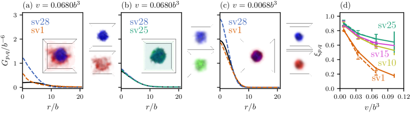
Figure 2: FTS-computed PDFs and mixing parameter $\xi_{p,q}$ for binary sv sequence mixtures. (a–c) Each $G_{p,p}$, $G_{q,q}$ (dashed, in color) and $G_{p,q}$ (solid, black) for the indicated $v$ is computed using a periodic $48^{3}$ mesh averaged over 30–40 independent runs (standard errors comparable to the plotting line width). Inset are illustrative snapshots of the real non-negative part of the density operators $\tilde{\rho}_{\rm{b},p}$ and $\tilde{\rho}_{\rm{b},q}$ depicted in different colors; the component species in the same snapshot are shown separately on the side. (d) $\xi_{p,q}$ is computed using a periodic $32^{3}$ mesh (averaged over 70–80 independent runs, solid lines) as well as the $48^{3}$ mesh (dashed lines) used for (a–c). Error bars represents standard errors of the mean.

PDFs indicate that significant charge pattern mismatch and strong $v$ are both necessary for demixing. Representative results are shown in Fig. 2 (see Appendix and Supplemental Material for comprehensive results). The strongest demixing is observed for sv28–sv1 with large charge pattern mismatch (SCDs differ by 15.58) at relatively high $v$ values; e.g., for $v=0.068b^{3}$, $G_{\mathrm{sv1},\mathrm{sv28}}(r)$ takes much lower values than $G_{\mathrm{sv1},\mathrm{sv1}}(r)$ and $G_{\mathrm{sv28},\mathrm{sv28}}(r)$ as $r\to 0$ (Fig.2a), indicating that some of the $\mathrm{sv1}$ chains are expelled from the sv28-dense region. Even when a single droplet is formed, it harbors sub-regions where either $\mathrm{sv28}$ or $\mathrm{sv1}$ dominates (snapshot in Fig.2a). However, when $v$ decreases to $0.0068b^{3}$, all three $G$s for sv28–sv1 share similar profiles, implying that the common droplet is well mixed (Fig.2c). In contrast, for sv28-sv25 with similar charge patterns (SCDs differ by $3.22$), mixing in the phase-separated droplet remains substantial even at higher $v$ (Fig. 2b). The general trend is summarized by the mixing parameter (Fig. 2d)

$$\xi_{p,q}\equiv\frac{2\rho^{0}_{{\mathrm{b}},p}\rho^{0}_{{\mathrm{b}},q}G_{p,q}(0)}{(\rho^{0}_{{\mathrm{b}},q})^{2}G_{p,p}(0)+(\rho^{0}_{{\mathrm{b}},p})^{2}G_{q,q}(0)}\;,$$ (16)

which vanishes for two perfectly demixed species, because in that case at least one of the factors in $\hat{\rho}_{\mathrm{b},p}(\bm{r})\hat{\rho}_{\mathrm{b},q}(\bm{r})$ would be zero for any $\bm{r}$, whereas $\xi_{p,q}=1$ when $\hat{\rho}_{\mathrm{b},p}(\bm{r})\propto\hat{\rho}_{\mathrm{b},q}(\bm{r})$, i.e., when the species are perfectly mixed.

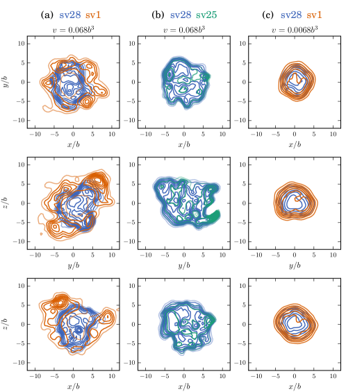
Figure 3: Cross-sections of FTS droplets of binary sv sequence mixtures illustrating the interplaying roles of sequence charge pattern mismatch and generic excluded volume in mixing/demixing of polyampholyte species. Shown here are two-dimensional slides through the droplet center of mass in the $x$–$y$ (top), $y$–$z$ (middle), and $x$–$z$ (bottom) planes for the three FTS droplets depicted in Fig. 2a–c. Density contours for the two sv sequence components $p,q$ in a given mixture are color coded as indicated by the labels at the top of the (a)–(c) columns. The contours for species $p$ ($q$) are curves of constant bead density, where “bead density” here in a FTS snapshot means the real non-negative part of the density operator, viz., $\Re_{+}(\tilde{\rho}_{\mathrm{b},p/q}(\bm{r}))$ where $\Re_{+}(u)\equiv[\Re(u)+{\rm sign}(\Re(u))]/2$ for any complex number $u$. (Among all snapshots considered, $\Re(\tilde{\rho}_{\mathrm{b},p}(\bm{r}))<-0.01b^{-3}$ occurs only for $<2\%$ of the mesh points). The contours are evenly spaced from $\Re(\tilde{\rho}_{\mathrm{b},p})$, $\Re(\tilde{\rho}_{\mathrm{b},q})$ $=$ $0$ [transparent] to $\Re_{+}(\tilde{\rho}_{\mathrm{b},p})$ $=$ $\max\{\Re_{+}(\tilde{\rho}_{\mathrm{b},p})\}$ ($\Re_{+}(\tilde{\rho}_{\mathrm{b},q})$ $=$ $\max\{\Re_{+}(\tilde{\rho}_{\mathrm{b},q})\}$) [opaque] where $\max\{\Re_{+}(\tilde{\rho}_{\mathrm{b},p})\}$ ($\max\{\Re_{+}(\tilde{\rho}_{\mathrm{b},q})\}$) is the maximum density of species $p$ ($q$) in a given snapshot.

The dual requirements of a significant sequence charge pattern mismatch and a substantial generic excluded volume for demixing of two polyampholyte species in a condensed droplet are illustrated by the FTS snapshots for the sv28-sv1 pairs ($v/b^{3}=0.068$ and $0.0068$) and sv28-sv25 pairs ($v/b^{3}=0.068$) in Fig. 2a–c. Those snapshots present an overall view from the outside of the droplet. Thus, part of their interior structure is obscured, albeit this limitation is partly remedied by the translucent color scheme. Further analyses to better understand the internal structures of these FTS snapshots are provided by the cross-sectional views in Fig. 3. The contour plots in Fig. 3a for the sv28-sv1 system with a high generic excluded volume strength show clearly that there is indeed a three-dimensional core with highly enriched sv28 population surrounded by a shell with enriched sv1 population. In contrast, the contour plots for the sv28-sv25 system at the same excluded volume strength (Fig. 3b) and the sv28-sv1 system at a low generic excluded volume strength (Fig. 3c) indicate that the two polyampholytes species are quite well mixed in the condensed droplets of these two systems. Nonetheless, the patterns of the contours reveals that even for these well-mixed systems, sv28 is still slightly more enriched in the core and the other sv sequence is slightly more enriched in a surrounding shell region.

IV Explicit-chain coarse-grained molecular dynamics (MD) simulations

While field theory affords deep physical insights, its ability to capture certain structure-related features pertinent to polyampholyte LLPS, such as the interplay between excluded volume and Coulomb interactions, can be limited Das et al. (2018b). To assess the robustness of the above FTS-predicted trend, we now turn to explicit-chain MD to simulate binary mixtures of the same sv sequence pairs as with FTS, using an efficient protocol involving initial compression and subsequent expansion of a periodic simulation box for equilibrium Langevin sampling Silmore et al. (2017); Dignon et al. (2018a); Das et al. (2018b). Each of our MD systems contains 500 chains equally divided between the two sv sequences (250 chains each). The LJ parameter $\epsilon$ that governs excluded volume is set at $\epsilon=l_{\rm B}/a_{0}$ (corresponding to the “with 1/3 LJ” prescription in Das et al. (2018b)), $T^{*}\equiv(\beta\epsilon)^{-1}$ is reduced temperature, and a stiff force constant $K_{\rm b}=75,000\epsilon/a_{0}^{2}$ for polymer bonds is employed as in Silmore et al. (2017); Das et al. (2018b). We compare results from using van der Waals radius $r_{0}=a_{0}$ (as before Das et al. (2018b)) and $r_{0}=a_{0}/2$ to probe the effect of excluded volume. Simulations are conducted at $T^{*}=0.6$ and $T^{*}=4.0$, which is, respectively, below and above the LLPS critical temperatures of all sv sequences in Fig. 1 in our MD systems, and at an intermediate $T^{*}$.

All MD simulations are performed using the GPU version of HOOMD-blue simulation package Anderson et al. (2008); Glaser et al. (2015) as in Das et al. (2018b). For systems with excluded volume parameter $r_{0}=a_{0}$ (all systems considered except in one case where we used $r_{0}=a_{0}/2$), we initially randomly place all the polyampholyte chains inside a sufficiently large cubic simulation box of length $70a_{0}$. The system is then energy minimized using the inbuilt FIRE algorithm to avoid any steric contact for a period of $500\tau$ with a timestep of $0.001\tau$, where $\tau\equiv\sqrt{ma^{2}/\epsilon}$ and $m$ is the mass of each bead (representing a monomer, or residue). Each system is first initiated at a higher temperature—at a high $T^{*}=4.0$—for a period of $5,000\tau$. The box is then compressed at $T^{*}=4.0$ for a period of $5,000\tau$ using isotropic linear scaling until we reach a sufficiently higher density of $\sim 0.7ma_{0}^{-3}$ which corresponds to a box size of $33a_{0}\times 33a_{0}\times 33a_{0}$. Next, we expand the simulation box length along one of the three Cartesian directions (labeled $z$) 8 times compared to its initial length to reach a final box length of $264a_{0}$, hence the final dimensions of the box is $33a_{0}\times 33a_{0}\times 264a_{0}$. For the system investigated for the effect of reduced excluded volume with $r_{0}=a_{0}/2$, the initial compressed box size is $20a_{0}\times 20a_{0}\times 20a_{0}$, and the final box size is $20a_{0}\times 20a_{0}\times 160a_{0}$. The box expansion procedure is conducted at a sufficiently low temperature of $T^{*}=0.4$. After that, each system is equilibrated again at the desired temperature for a period of $30,000\tau$ using Langevin dynamics with a weak friction coefficient of $0.1m/\tau$ Silmore et al. (2017). Velocity-Verlet algorithm is used to propagate motion with periodic boundary conditions for the simulation box. Production run is finally carried out for $100,000\tau$ and molecular trajectories are saved every $10\tau$ for subsequent analyses.

For density distribution calculations, we first adjust the periodic simulation box in such a way that its centre of mass is always at $z=0$. The simulation box is then divided along the $z$-axis into 264 bins of size $a_{0}$ for $r_{0}=a_{0}$ or 160 bins of size $a_{0}$ for $r_{0}=a_{0}/2$ to produce a total density profile as well as profiles for the two individual polyampholyte species in the binary mixture. As for the $G_{p,q}(|\bm{r}-\bm{r}^{\prime}|)$ in FTS, in the calculation of the MD-simulated $G_{p,q}(|\bm{r}-\bm{r}^{\prime}|)$ from configurations in the MD simulation box with periodic boundary conditions, $|\bm{r}-\bm{r}^{\prime}|$ is taken to be the shortest distance of the possible inter-bead distances determined in the presence of periodic boundary conditions.

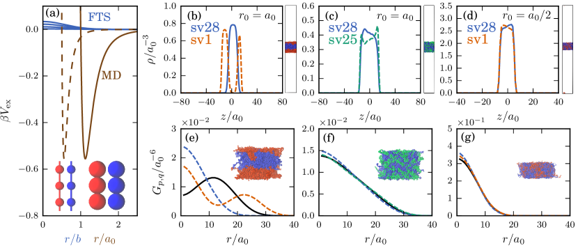
Figure 4: MD-simulated LLPS of binary sv sequence mixtures. (a) Excluded volume interactions in FTS (blue) for $v/b^{3}$ $=$ $0.102$, $0.068$, $0.034$, and $0.0068$ (top to bottom, independent of $T^{*}$) and in MD (brown) for $r_{0}=a_{0}$ (solid) and $r_{0}=a_{0}/2$ (dashed) at $T^{*}=0.6$ (insets show relative sizes of the LJ spheres). (b)–(d) MD-simulated polyampholyte densities of binary mixtures, $\rho(z)$s for different sv sequences are colored differently (as indicated) here and in the snapshots (on the side) of the rectangular periodic simulation boxes (wherein $z$ is the vertical coordinate), each harboring a condensed droplet. (e)–(g) $G_{p,q}$ of the MD systems in (b)–(d), respectively, (same line style as Fig. 2a–c). Droplet snapshots (insets) are visualized Humphrey et al. (1996) here with chains at periodic boundaries unwrapped.

A substantive difference between common FTS and MD is in their treatment of polymer excluded volume, as illustrated in Fig. 4a for the present models, wherein $\beta V_{\rm ex}(r)$ is the excluded-volume interaction, given by $\beta{\hat{H}}_{1}$ in Table 1, for a pair of beads centered at $\bm{r}_{p,i,\alpha}$ and $\bm{r}_{q,j,\gamma}$, with $r=|\bm{r}_{p,i,\alpha}-\bm{r}_{q,j,\gamma}|$. For our FTS model as well as several recent FTS studies McCarty et al. (2019); Lin et al. (2019); Danielsen et al. (2019a),

$$\beta V_{\rm ex}(r)=\frac{v}{2}\int\mathrm{d}\bm{r}\Gamma(\bm{r}-\bm{r}_{p,i,\alpha})\Gamma(\bm{r}-\bm{r}_{q,j,\gamma})=v\left(\frac{1}{4\pi a^{2}}\right)^{3/2}\exp\left(-\frac{r^{2}}{4a^{2}}\right)\quad\mbox{(FTS)}\,,$$ (17)

is a Gaussian, which allows the beads to overlap completely ($r=0$), albeit with a reduced yet non-negligible or even moderately high probability. In contrast, for MD,

$$\beta V_{\rm ex}(r)=\frac{4}{3T^{*}}\left[\left(\frac{r_{0}}{r}\right)^{12}-\left(\frac{r_{0}}{r}\right)^{6}\right]\quad\mbox{(MD),}$$ (18)

which entails a repulsive wall at $\sim r_{0}$ that is all but impenetrable, let alone an excluded-volume-violating complete overlap. Note that if the $\beta V_{\rm ex}(r)$ for MD is shown for $T^{*}=0.2$ (as for FTS) instead of $T^{*}=0.6$ in Fig. 4a, the contrast would be even more overwhelming between FTS and MD excluded-volume prescriptions.

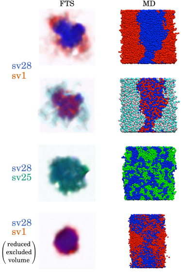
Figure 5: Cross-sectional views of FTS and MD snapshots of binary mixtures of polyampholytes afford a consistent picture of sequence- and excluded-volume-dependent droplet organization. (Left) FTS density distributions on one of the two-dimensional planes in Fig. 3 through each droplet’s center of mass. (Right) Corresponding cut-out views of the MD droplets shown inside the periodic simulation boxes in Figs. 4b–d at one half of the box dimension extending perpendicularly into the page. Two different representations are used to visualize the sv28-sv1 droplet with full excluded volume (top two rows; $v=0.068b^{3}$, $r_{0}=a_{0}$). Upper row: sv1 and sv28 are depicted, respectively, in red and blue. Lower row: The negatively and positively charged beads in sv28 are depicted, respectively, in red and blue, whereas the corresponding beads in sv1 are depicted in pink and cyan. The color code for the sv28-sv25 mixture at full excluded volume (third row from top; $v=0.068b^{3}$, $r_{0}=a_{0}$) and the sv28-sv1 mixture with reduced excluded volume (bottom row; $v=0.0068b^{3}$, $r_{0}=a_{0}/2$) follows that in Figs. 2 and 4.

Despite this and other differences between MD Radhakrishna et al. (2017); Rathee et al. (2018); Madinya et al. (2020) and field theory Danielsen et al. (2019a, b) that preclude a direct comparison of MD and FTS excluded volume, it is reassuring that MD and FTS predictions on sequence-pattern and excluded-volume dependent condensed-phase mixing/demixing share the same trend. Results for sv28–sv1 and sv28–sv25 are shown in Fig. 4b–g for $T^{*}=0.6$ to illustrate a perspective that is buttressed by additional MD results in the Appendix and Supplemental Material for other sequence pairs, other $T^{*}$s, their $\xi_{p,q}$ mixing parameters (Eq. 16), and $r_{0}=a_{0}/2$ sequences with proportionally reduced charged interactions.

Fig. 4b–d show the average densities $\rho(z)$ along the long axis, $z$, of the simulation box. With full excluded volume and significant charge pattern mismatch, sv28 and sv1 strongly demix in the condensed phase (cf. blue and red curves in Fig. 4b). In contrast, without a significant charge pattern mismatch, even with full excluded volume, sv28 and sv25 are quite well mixed (blue and green curves largely overlap in Fig. 4c); and, with reduced excluded volume, even sv28 and sv1 with significant charge pattern mismatch are well mixed (Fig. 4d).

This trend is echoed by the PDFs in Fig. 4e–g, each computed from 10,000 MD snapshots. For the well-mixed cases in Fig. 4f,g, the MD-computed self ($G_{p,p}$, $G_{q,q}$) and cross ($G_{p,q}$) PDFs largely overlap, similar to those in Fig. 2b,c for FTS. For the sv28–sv1 pair with full excluded volume in MD, Fig. 4e shows that $G_{p,q}(r)$ is significantly smaller than $G_{p,p}(r)$ and $G_{q,q}(r)$ for small $r$, as in Fig. 2a for FTS. Here, the MD $G_{q,q}$ for sv1 exhibits a local maximum at $r\approx 23a_{0}$ corresponding to the distance between two sv1 density peaks in Fig. 4b. This feature reflects the anisotropic nature of the rectangular simulation box adopted to facilitate efficient sampling Silmore et al. (2017). Nonetheless, the geometric arrangement of sv28 and sv1 in the MD system, as visualized by the snapshot in Fig. 4e, is consistent with that in Fig. 2a for FTS in that an sv28-enriched core (blue) is surrounded by an sv1-enriched (red) periphery in both cases. The other MD snapshots in Fig. 4f,g depict well-mixed droplets, similar to the corresponding FTS snapshots in Fig. 2b,c.

The MD-simulated droplet snapshots at low temperature $T^{*}=0.6$ in Figs. 4b–g underscore that demixing of two polyampholyte species in a condensed droplet requires a significant mismatch in sequence charge pattern as well as a substantial excluded volume repulsion. Because the beads (monomers) are represented in our MD drawings as opaque spheres, the bulk of those droplets below the surface of the image presented cannot be visualized. To better illustrate that the observed mixing/demixing trend applies not only to the exterior of the presented image of those droplets but persists in the parts underneath (as can be inferred by the behaviors of $G_{p,p}$, $G_{q,q}$, and $G_{p,q}$ in Figs. 4e–g), we prepare cut-out images of those droplets to reveal the spatial organization in their “core” regions (Fig. 5). The spatial configurations of the MD droplets and their general trend of behaviors (Fig. 5, right column) are very similar to those exhibited by cross-sectional views of FTS droplets (contour plots in Fig. 3 and density plots in Fig. 5, left column), demonstrating once again the robustness of our observations. By construction, MD provides much more spatial details than FTS in this regard. Of particular future interest is the manner in which individual positively and negatively charged beads interact across polyampholytes of different species. MD snapshots should be useful for elucidating this issue. In contrast, although FTS snapshots—with their cloudy appearances—may show a similar spatial organization of charge densities as that of MD, the field configurations do not translate into individual bead positions (Fig. 5, second row).

V Conclusion

Excluded volume has been shown to attenuate complex Perry and Sing (2015) and simple McCarty et al. (2019) coacervation (i.e., excluded volume generally disfavors demixing of solute and solvent) but to promote demixing of molecular (solute) components when applied differentially to different molecular components in a condensate Harmon et al. (2018). Here, going beyond these and other effects of excluded volume on the organization of condensed matter (e.g., nanogel Adroher-Ben\́mathrm{missing}itez et al. (2017) and polymer-nanoparticle systems Sorichetti et al. (2018)), FTS and MD both demonstrate a hitherto unrecognized stochastic molecular recognition principle, that a uniform excluded volume not discriminating between polymer species can nonetheless promote condensed-phase demixing and that a certain threshold excluded volume is required for heteropolymers with different sequence charge patterns to demix upon LLPS. Our MD results show clearly that sequences such as sv28 and sv1 that are not obviously repulsive to each other can nevertheless demix in the condensed phase, supporting RPA predictions that such demixing of different species of overall neutral polyampholytes depends on charge pattern mismatch Lin et al. (2017a). In light of the present finding, this success of RPA in Lin et al. (2017a) may be attributed to the incompressibility constraint—which presupposes excluded volume—in its formulation. Surprisingly, although the FTS excluded volume repulsion we consider is exceedingly weak—the highest $v$ only amounts to $\sim 0.03k_{\mathrm{B}}T$ maximum and thus can easily be overcome by thermal fluctuations (Fig. 4a), the demixing observed in FTS with this $v$ is similar to that in MD with a much stronger, more realistic excluded volume. While the theoretical basis of this reassuring agreement, e.g., its possible relationship with the treatment of chain entropy in FTS, remains to be ascertained, our observation that sv28 and sv1 do not demix at a lower $v$ points to potential limitations of employing small $v$ values in FTS.

These basic principles offer new physical insights into subcompartmentalization of membraneless organelles, in terms of not only the sequence charge patterns of their constituent IDPs Lin et al. (2017a), but also of excluded volumes entailed by amino acid sidechains of various sizes, volume increases due to posttranslational modifications such as phosphorylations Kim et al. (2019), presence of folded domains, and the solvation properties of the IDP linkers connecting these domains Li et al. (2012); Harmon et al. (2018). Guided by this conceptual framework, quantitative applications to real-life biomolecular condensates require further investigations to consider sequences that are not necessarily overall charge neutral Lin et al. (2020), and to incorporate non-electrostatic driving forces for LLPS such as $\pi$-related Vernon et al. (2018) and hydrophobic Statt et al. (2020); Zheng et al. (2020) interactions. Much awaits to be discovered.

ACKNOWLEGMENTS

We thank Yi-Hsuan Lin for insightful discussions, and gratefully acknowledge support by Canadian Institutes of Health Research grant NJT-155930, Natural Sciences and Engineering Research Council of Canada Discovery grant RGPIN-2018-04351, and computational resources from Compute/Calcul Canada.

T.P. and J.W. contributed equally to this work.

APPENDIX: COMPREHENSIVE FTS AND MD RESULTS, PAIR
CORRELATION FUNCTIONS AND SECOND VIRIAL COEFFICIENTS

In this Appendix, figures with number labels preceded by “S” refer to the figures in Supplemental Material.

A. Comprehensive FTS results

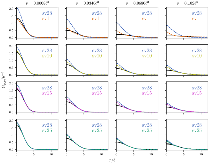
Figure S1: PDFs of binary mixtures of sv sequences computed by FTS using a $32^{3}$ mesh at $l_{\rm B}=5b$ ($T^{*}=0.2$) and various $v$. The plotting style follows that of Fig. 2 main text. Dashed blue curves: $G_{p,p}(r)$ for sv28 ($-$SCD=$15.99$); dashed color curves: $G_{q,q}(r)$ for (top to bottom) sv1, sv10, sv15, and sv25 ($-$SCD=$0.41$, $2.10$, $4.35$, and $12.77$, respectively); solid black curves: $G_{p,q}(r)$. The shaded region around each curve represents standard error of the mean among the $\sim 80$ independent runs for each system, which is mostly smaller than the width of the curve.

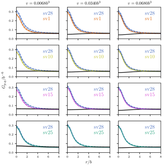
Figure S3: PDFs of binary mixtures of sv sequences computed by FTS using a $32^{3}$ mesh or a $48^{3}$ mesh at $l_{\rm B}=0.05b$ ($T^{*}=20.0$). Dashed (dotted) blue curves: $G_{p,p}(r)$ for sv28 from a $48^{3}$ ($32^{3}$) mesh; dashed (dotted) color curves: $G_{q,q}(r)$ for (top to bottom) sv1, sv10, sv15, and sv25 from a $48^{3}$ ($32^{3}$) mesh; solid (dotted) black curves: corresponding $G_{p,q}(r)$ obtained using a $48^{3}$ ($32^{3}$) mesh. At this high temperature, the behaviors of all systems are very similar irrespective of the sequence charge patterns or excluded volume interaction $v$ values considered. The $r/b$ scale is enlarged vis-à-vis Figs. S1 and S2 to make the differences between the plotted curves here visible.

Figs. S1 and S2 show PDFs of all of the sv sequence pairs considered in the present work. They are computed using, respectively, the $32^{3}$ and $48^{3}$ meshes under various excluded volume strengths $v$. Results are available for the highest $v/b^{3}=0.102$ we simulated for the $32^{3}$ mesh but not for the $48^{3}$ mesh because equilibration is problematic for the larger mesh at strong excluded volume. At the low temperature ($l_{\rm B}=5b$, $T^{*}=0.2$) at which these simulations are conducted, a hallmark for the existence of a condensed droplet is the decay of the $G_{p,p}$, $G_{q,q}$, and $G_{p,q}$ functions to $\approx 0$ at $r\approx 10b$; and a significant demixing of the populations of the two sequence species is signaled by a substantially lower $G_{p,q}(r)$ ($p\neq q$), for small $r\approx 0$, than both $G_{p,p}(r)$ and $G_{q,q}(r)$ in the same range of $r$. The trends exhibited by the two sets of results in Figs. S1 and S2 are consistent. They indicate robustly that both a significant difference in sequence charge pattern of the two polyampholyte species (difference decreases from the sv28-sv1 to the sv28-sv25 pair) and a substantial excluded volume (relatively large $v$ values) are required for appreciable demixing. This observation corroborates the trend illustrated by the sv28-sv1 and sv28-sv25 examples and the $\xi_{p,q}$ measure presented in Fig. 2. As a control, and not surprisingly, when FTS is conducted at a much higher temperature of $T^{*}=20$ ($l_{\rm B}=0.05b$) in Fig. S3 , there is little sequence dependence—as seen by the very similar behaviors of all $G_{p,p}(r)$, $G_{q,q}(r)$, and $G_{p,q}(r)$ among the sequence pairs considered—and there is no droplet formation. Instead of converging to zero at large $r$ as in Figs. S1 and S2, here all $G(r)$s converge to a finite (nonzero) value of $\langle\hat{\rho}_{\mathrm{b},p}\rangle_{\mathrm{P}}\langle\hat{\rho}_{\mathrm{b},q}\rangle_{\mathrm{P}}\approx 0.05b^{-6}$ at large $r$ in Fig. S3 for $p\neq q$ as well as $p=q$, signalling a total lack of correlation between distant beads.

B. Comprehensive MD results

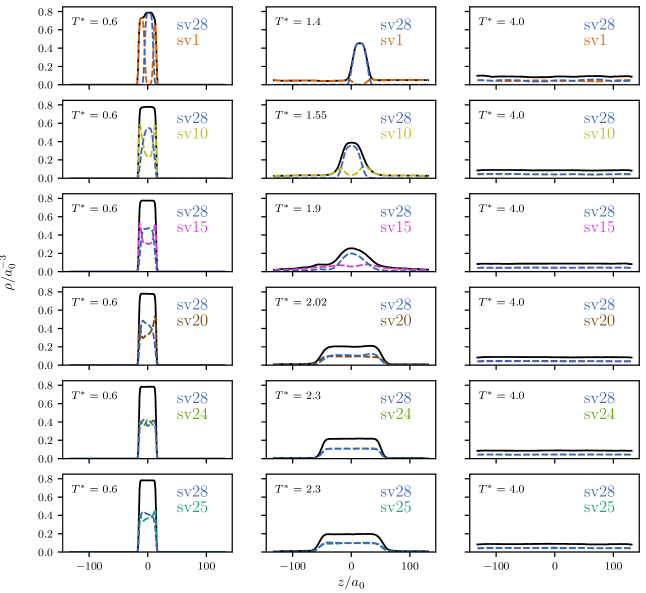
Figure S4: MD-simulated average density of binary mixtures of sv sequences along the $z$ (long) axis of the simulation box at various temperatures for $r_{0}=a_{0}$. Solid curves: total bead density; color dashed curves: density of individual sv polyampholyte species. In addition to the four sv pairs studied using FTS, MD results for the sv28-sv20 ($-$SCD = $15.99,7.37$) and sv28-sv24 ($-$SCD = $15.99,17.00$) pairs are obtained to cover the six sv pairs studied using RPA in Y.-H. Lin, J. P Brady, J. D. Forman-Kay, and H. S. Chan, New J. Phys. 19, 115003 (2017).

Fig. S4 shows the density profiles of six sv sequence pairs (the same sv pairs analyzed using RPA in Ref. Lin et al. (2017a)). At a sufficiently low temperature of $T^{*}=0.6$, LLPS is observed for all $r_{0}=a_{0}$ systems simulated here, in that a droplet, manifested as a density plateau, is observed (left column of Fig. S4). At this low temperature, demixing of the two species in the binary mixture is clearly observed for sv28-sv1 and sv28-sv10, and nearly complete mixing is observed for sv28-sv24 and sv28-sv25. Intermediate behaviors that may be characterized as partial demixing—with sv28 slightly enriched in the middle and the other sequence species slightly enriched on the two sides—are observed for sv28-sv15 and sv28-sv20. The trend is also seen at intermediate temperatures ($T^{*}=1.4$–$2.3$). However, in some of these cases, one of the polyampholytes either does not (e.g. sv1) or barely (e.g. sv15) phase separate, as indicated by the long “tails” of their density profile outside the central region (middle column of Fig. S4). Not unexpectedly, at a high temperature of $T^{*}=4.0$, none of the simulated systems phase separates and the two species are mixed homogeneously throughout the simulation box (right column of Fig. S4).

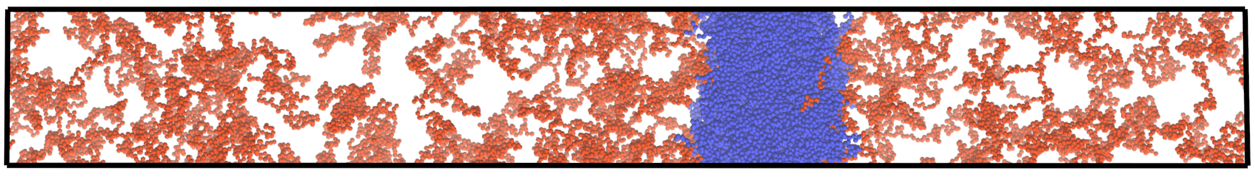
(a) sv28-sv1, $T^{*}=1.4$

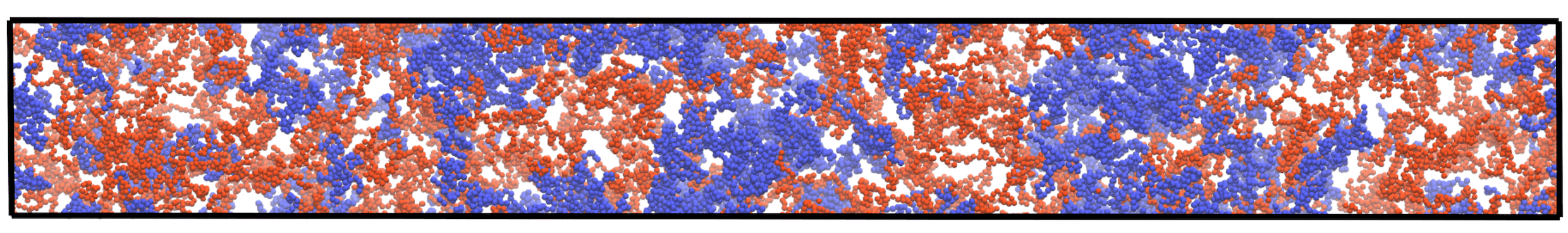
(b) sv28-sv1, $T^{*}=4.0$

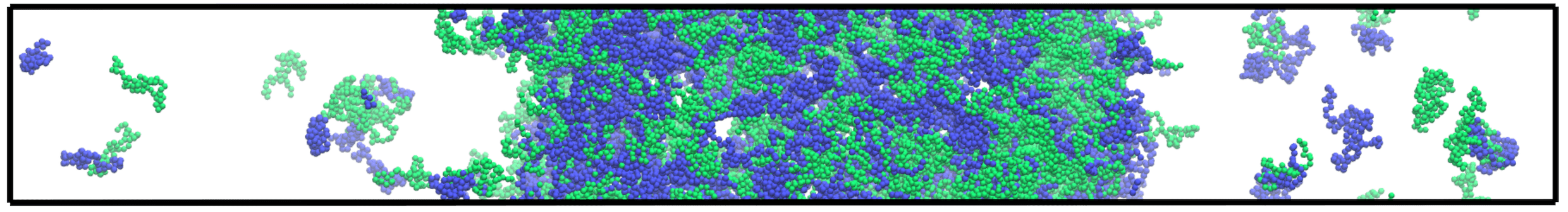
(c) sv28-sv25, $T^{*}=2.3$

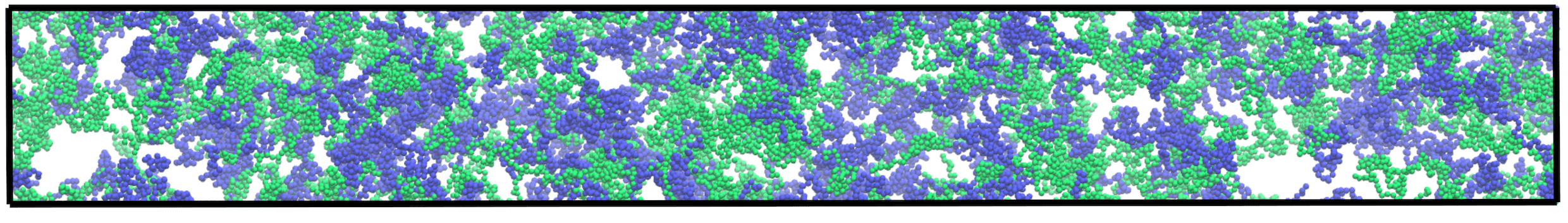
(d) sv28-sv25, $T^{*}=4.0$

Figure S6: Simulation snapshots of binary mixtures of sv sequences at the reduced temperatures indicated. Polyampholyte chains with charge sequences sv28, sv1, and sv25 are depicted, respectively, in blue, red, and green.

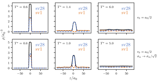
Figure S7: MD-simulated average density of binary mixtures of sv28 and sv1 along the $z$ (long) axis of the simulation box at various temperatures for $r_{0}=a_{0}/2$. Solid curves: total bead density; color dashed curves: density of individual sv polyampholyte species; same line style as that in Fig. S4. Top: Results from the $r_{0}=a_{0}/2$ system described in the main text. Bottom: Results from a simulation wherein the electric charge on each of the beads in the sv sequences is scaled by a factor of $1/\sqrt{2}$ such that the electrostatic interaction energies for two contacting beads in this $r_{0}=a_{0}/2$ system is identical to that in the original $r_{0}=a_{0}/2$ system with the original (unscaled) charges on the beads.

These trends are summarized quantitatively in Fig. S5 using essentially the same $\xi_{p,q}$ parameter defined in Eq. (16). Consistent with the FTS results in Fig. 2, demixing of condensed-phase polyampholyte species increases with sequence charge pattern mismatch and increasing excluded volume. Representative snapshots of our MD-simulated systems are shown in Fig. S6. To highlight the impact of excluded volume, the $\xi_{p,q}$ parameter for the sv28–sv1, $r_{0}=a_{0}/2$ system with reduced excluded volume (Figs. 4d,g) is also shown in Fig. S5 (red cross), exhibiting once again that when $r_{0}=a_{0}/2$, sv28 and sv1 remain well mixed (do not demix) when a droplet is formed at low temperature (Fig. S7, top), these sequences’ significant difference in charge pattern notwithstanding, as has been shown by the pair distribution functions $G_{p,q}(r)$ in Fig. 4g.

To explore the potential impact of a stronger electrostatic interactions at contact—because of the reduced excluded volume—on this lack of demixing, we further simulate a control system in which the charge on each bead of the polyampholyte chains is scaled by a factor of $1/\sqrt{2}$ such that the electrostatic interaction energy when two beads are in contact in the $r_{0}=a_{0}/2$ system is the same as that in the original $r_{0}=a_{0}$ system. Simulation results of this control system show that aside from minor differences, the two species—sv28 and sv1—remain well mixed in the phase-separated droplet (Fig. S7 , bottom-left). This result, together with the recognition that beads on polyampholytes with $r_{0}=a_{0}/2$ can interdigitate because the bonds connecting the chains have no excluded volume (Fig. 4a, inset) and therefore likely allow for more mixing of polyampholyte species, confirms once again that excluded volume, overall, is a prominent driving factor for demixing of polyampholyte species in the condensed phase.

C. Pair distribution functions and second virial coefficients

Virial expansion is a perturbative approach useful for studying nonideal gas and dilute solution as it is a power series in density (concentration) Pathria (1972). The coefficient of the second term in the expansion of mechanical or osmotic pressure, known as the second virial coefficient and often denoted as $B_{22}$ or $B_{2}$, may be expressed as

$$B_{2}=2\pi\int_{0}^{\infty}\mathrm{d}r\;r^{2}\left(1-\mathrm{e}^{-\beta U_{2}(r)}\right)=2\pi\int_{0}^{\infty}\mathrm{d}r\;r^{2}\left[1-g_{\rm dil}(r)\right]$$ (A1)

for an isotropic pairwise potential $U_{2}(r)$, and the second equality follows when $g_{\rm dil}$ is the normalized radial distribution in the limit of infinite dilution because $g_{\rm dil}(r)=\exp[-\beta U_{2}(r)]$ [$g_{\rm dil}(r)\rightarrow 1$ as $r\rightarrow\infty$] Neal et al. (1998). As such, $B_{2}$ is particularly useful for characterizing the interactions between two otherwise isolated molecules Dignon et al. (2018b); Amin et al. (2020); but is insufficient for an accurate account at high densities or high solute concentrations because contributions involving third and higher orders in density are neglected.

In contrast, the pair distribution functions (PDFs) computed in this work are exact (inasmuch as the finite-size model systems considered are concerned). For this reason, and in this regard, the configurational information contained in PDFs is superior to that of $B_{2}$. Our PDFs are nonperturbative, and therefore they provide an accurate characterization of the mixing/demixing of polyampholytes species in both the dilute and condensed phases. To further compare and contrast the PDFs [$G_{p,q}(r)$ defined in Eq. (1) ] in the present formulation and $B_{2}$, it is instructive to define an exact radial distribution function,

$$g_{p,q}(r)\equiv\frac{G_{p,q}(r)}{\rho^{0}_{{\rm b},p}\rho^{0}_{{\rm b},q}}\,$$ (A2)

for our FTS as well as MD systems. Unlike the aforementioned $g_{\rm dil}(r)$, here $g_{p,q}(r)$ is not restricted to the dilute phase. Using $g_{p,q}(r)$ in place of $g_{\rm dil}(r)$ in Eq. A1, we may construct a second virial coefficient-like quantity

$${\widetilde{B}}^{(2)}_{p,q}\equiv\frac{1}{2}\int_{0}^{r_{\mathrm{max}}}\mathrm{d}r\,V(r/L)\left[1-g_{p,q}(r)\right]\,,$$ (A3)

where $L$ is the side length of the simulation box. As in a recent simulation study of biomolecular condensates Choi et al. (2019), $V(r/L)$ is used to adapt the integration measure to the periodic boundary conditions of a cubic simulation box, where

$$V(x) = \left\{\begin{matrix}4\pi x^{2}\,,&0\leq x\leq 1/2\,,\\ 2\pi x(3-4x)\,,&1/2<x\leq\sqrt{2}/2\,,\\ 2x(3\pi-12f_{1}(x)+f_{2}(x))\,,&\sqrt{2}/2<x\leq\sqrt{3}/2\,,\end{matrix}\right.$$ (A4)

$$f_{1}(x) = \tan^{-1}\sqrt{4x^{2}-1}\,,$$ (A5)

$$f_{2}(x) = 8x\left\{\tan^{-1}\left[\frac{2x(4x^{2}-3)}{\sqrt{4x^{2}-2}(4x^{2}+1)}\right]\right\}\,.$$ (A6)

The above equations are Eqs. 18 and 19 in Ref. Choi et al. (2019) (note, however, that our $g_{p,q}(r)$ is different from their ${\tilde{g}}(r)$ because of different normalizations).

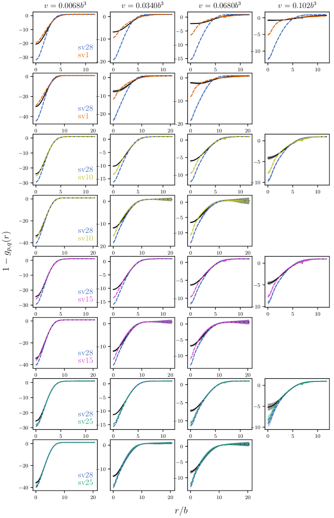
Figure S8: Radial distribution functions of FTS phase-separated systems ($l_{\rm B}=5b$, $T^{*}=0.2$). Shown here is the function $1-g_{p,q}(r)$, where the normalized radial distribution $g_{p,q}(r)$ is defined by Eq. A2 in the Appendix of the main text with the pair distribution functions (PDFs), $G_{p,q}(r)$, given by Fig. S1 ($32^{3}$ mesh) and Fig. S2 ($48^{3}$ mesh). The line styles for $p,q$ are the same as in Figs. S1 and S2. Here, for the same sv-sequence pairs, the upper and the lower rows show $1-g_{p,q}(r)$ (which is the integrand for ${\widetilde{B}}^{(2)}_{p,q}$ given by Eq. A3 in the Appendix of the main text) for $32^{3}$ and $48^{3}$ meshes, respectively. Shown results computed using the two different mesh sizes are nearly identical. The error bars follow those for the $G_{p,q}(r)$s, rescaled here in accordance with Eq. A2 in the Appendix of the main text.

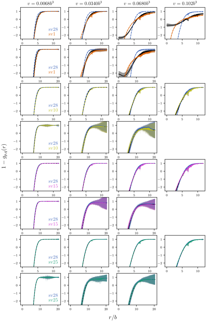
Figure S9: Zoomed-in view of the radial distribution functions of FTS phase-separated systems. Same as Fig. S8 but now with a zoomed-in view around $1-g_{p,q}(r)=0$. In all cases, $1-g_{p,q}(r)\approx 1$ [i.e., $g_{p,q}(r)\approx 0$)] at large $r$.

The $1-g_{p,q}(r)$ expressions (in the integrand of Eq. A3) for our FTS systems are provided in Fig. S8 and Fig. S9. For these phase-separated systems, unlike the $1-g_{\rm dil}(r)$ in Eq. A1, $1-g_{p,q}(r)$ does not vanish at large $r$ because large $r$ invariably involves the dilute phase and hence these $g_{p,q}(r)\approx 0$, i.e., $1-g_{p,q}(r)]\approx 1$ for large $r$. Therefore, it is sensible to restrict the integration in Eq. A3 to the condensed phase, which may be implemented approximately by introducing an upper limit, $r_{\rm max}$, on the integration.

For $r_{\mathrm{max}}\leq L/2$, the volume integral reduces to the simple form

$${\widetilde{B}}^{(2)}_{p,q}\equiv 2\pi\int_{0}^{r_{\mathrm{max}}}\mathrm{d}r\,r^{2}\left[1-g_{p,q}(r)\right]\,,\quad r_{\mathrm{max}}\leq L/2\,.$$ (A7)

For the present MD systems, the final simulation boxes are not cubic, and the dimensions of the condensed phase is approximately $L^{3}$ where $L$ is the length of the shorter side of the simulation box ($L=33a_{0}$ for $r_{0}=a_{0}$ systems, $L=20a_{0}$ for $r_{0}=a_{0}/2$ systems; see Fig. 4b–g and discussion above). For this reason, $r_{\mathrm{max}}\leq L/2$ should be chosen for the MD systems. More generally, $r_{\rm max}$ may either be chosen as a pre-selected distance reflecting the size of the condensed droplet, or as the solution to the equation Choi et al. (2019)

$$g_{p,q}(r_{\mathrm{max}})=1\,.$$ (A8)

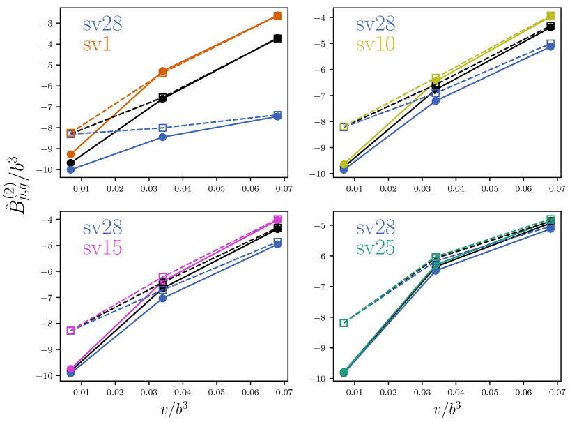
Figure S10: The second virial coefficient-like quantity ${\widetilde{B}}^{(2)}_{p,q}$ for various phase-separated FTS systems ($l_{\rm B}=5b$, $T^{*}=0.2$) each consisting of two polyampholyte species with different charge sequences (as indicated) computed using a $48^{3}$ mesh, as functions of the excluded volume parameter $v$. Filled circles represent ${\widetilde{B}}^{(2)}_{p,q}$ computed by Eq. A3 using an $r_{\rm max}$ that equals to the average of the three $r_{\rm max}$ values satisfying $g_{p,q}(r_{\rm max})=1$ (Eq. A8) for the $p,p$, $q,q$, and $p,q$ cases of the given pair of sequences. The open squares are ${\widetilde{B}}^{(2)}_{p,q}$ values computed using $r_{\rm max}=10b$ throughout. The solid and dashed lines connecting, respectively, the filled and open symbols are merely a guide for the eye.

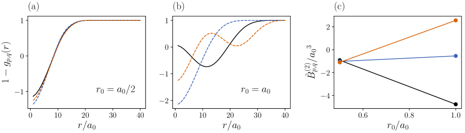
Figure S11: Comparing MD-simulated ${\widetilde{B}}^{(2)}_{p,q}$ of phase-separated systems with different excluded volume strengths. (a,b) The $1-g_{p,q}(r)$ functions for the sv28–sv1 MD systems are obtained, respectively, from the $G_{p,q}(r)$ functions in Fig. 4g ($r_{0}=a_{0}/2$) and Fig. 4e ($r_{0}=a_{0}$) of the main text (Eq. A2). The line styles for $p,p$, $q,q$, and $p,q$ are the same as in the main text figure. (c) The corresponding ${\widetilde{B}}^{(2)}_{p,q}$ values (same color code) are computed using $r_{\rm max}=10.0a_{0}$ for $r_{0}=a_{0}/2$ and $r_{\rm max}=16.5a_{0}$ for $r_{0}=a_{0}$. These $r_{\rm max}$ values amount to half of the length of the short sides of the systems’ simulation boxes. The solid lines connecting the $r_{0}=a_{0}/2$ and $r_{0}=a_{0}$ ${\widetilde{B}}^{(2)}_{p,q}$s are merely a guide for the eye.

We have computed ${\widetilde{B}}^{(2)}_{p,q}$ for our phase-separated FTS systems using different pre-selected $r_{\rm max}$ as well as $r_{\rm max}$s satisfying Eq. A8, and found that ${\widetilde{B}}^{(2)}_{p,q}$ is quite insensitive to reasonable variation in the choice of $r_{\rm max}$ as long as the choice captures approximately the size of the condensed droplet. Examples in Fig. S10 show that ${\widetilde{B}}^{(2)}_{p,q}$ for $p\neq q$ (black symbols) deviates more from ${\widetilde{B}}^{(2)}_{p,p}$ and/or ${\widetilde{B}}^{(2)}_{q,q}$ (symbols in other colors) with increasing sequence charge pattern mismatch and increasing excluded volume. The trend is most apparent for sv28–sv1 (Fig. S10 , top left) as this system entails a large sequence charge pattern mismatch. The trend observed in Fig. S10 of increased deviation of ${\widetilde{B}}^{(2)}_{p,q}$ for $p\neq q$ from those for $p=q$ with increasing excluded volume is echoed by the MD example in Fig. S11 as well. These examples underscore the fact that the configurational information afforded by the second virial coefficient-like quantity ${\widetilde{B}}^{(2)}_{p,q}$ is derived from $G_{p,q}(r)$ and therefore ${\widetilde{B}}^{(2)}_{p,q}$ and $G_{p,q}(r)$ carry similar messages; but because ${\widetilde{B}}^{(2)}_{p,q}$ involves an $r$-integration of $G_{p,q}(r)$, ${\widetilde{B}}^{(2)}_{p,q}$ averages out spatial details and thus contains less structural information of the system. As such, ${\widetilde{B}}^{(2)}_{p,q}$ is not as diagnostic as $\xi_{p,q}$ in probing mixing/demixing of polyampholyte components in the condensed phase (cf. Fig. 2d and Fig. S5). For that matter, as an integrated quantity, the second virial coefficient $B_{2}$ itself (Eq. A1) also provides less configurational information than $g_{\rm dil}(r)$.

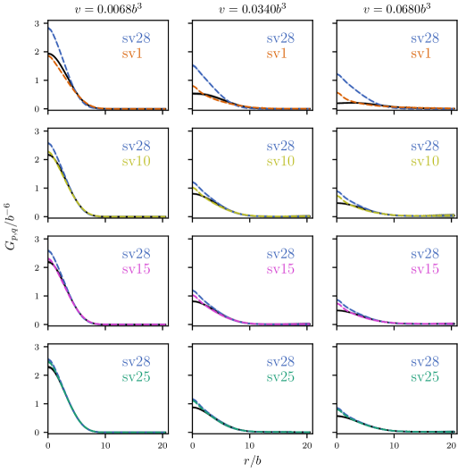
Figure S2: PDFs of binary mixtures of sv sequences computed by FTS using a $48^{3}$ mesh at $l_{\rm B}=5b$ ($T^{*}=0.2$). Results for each system are from $\sim 40$ independent runs. The notation is otherwise the same as that of Fig. S1.

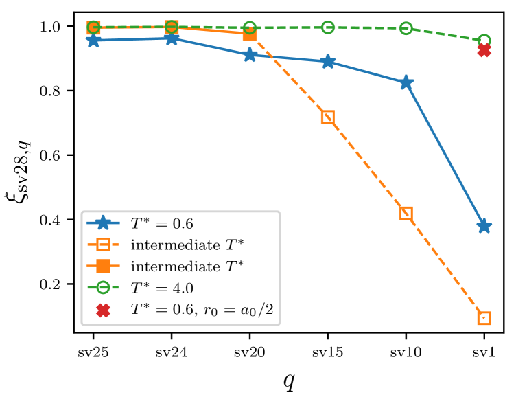
Figure S5: $\xi_{p,q}$ values for the $p=$sv28, $r_{0}=a_{0}$ MD systems in Fig. S4; with the $\xi_{{\mathrm{sv28}},{\mathrm{sv1}}}$ for $q=$sv1 and $r_{0}=a_{0}/2$ (Fig. S7, top-left) included for comparison (red cross). Since complete overlap of two beads ($r=0$) is all but impossible under the $r^{-12}$ excluded-volume term in the MD potential, the $G_{p,q}(0)$ values used to define $\xi_{p,q}$ in Eq. 16 of the main text are replaced by the nonzero $G_{p,q}$ values at the smallest $r$ sampled (cf. Fig. 4e–f of the main text) to compute the $\xi_{p,q}$ values plotted here. Intermediate $T^{*}$ are those reported in the middle column of Fig. S4. Systems with both polyampholyte species in the condensed phase are depicted by fill symbols, those with one or both species in the dilute phase (not condensed) are represented by open symbols. The solid and dashed connecting lines, respectively, through the filled and open symbols serve merely as a guide for the eye. Consistent with the FTS results in Fig. 2d of the main text, the trend of $\xi_{p,q}$ values shown here indicates clearly that the demixing of two polyampholyte species in a condensed phase (at low $T^{*}$) increases with increasing mismatch of their sequence charge patterns, and decreases with decreasing excluded volume (for sv1, the red cross indicates essentially no demixing whereas the blue star indicates strong demixing in the systems’ respective combined condensed phases of sv28 and sv1 at $T^{*}=0.6$).

References

- Brangwynne et al. (2009) C. P. Brangwynne, C. R. Eckmann, D. S. Courson, A. Rybarska, C. Hoege, J. Gharakhani, F. Jülicher, and A. A. Hyman, Science 324, 1729 (2009).
- Li et al. (2012) P. Li, S. Banjade, H. C. Cheng, S. Kim, B. Chen, L. Guo, M. Llaguno, J. V. Hollingsworth, D. S. King, S. F. Banani, P. S. Russ, Q.-X. Jiang, B. T. Nixon, and M. K. Rosen, Nature 483, 336 (2012).
- Kato et al. (2012) M. Kato, T. W. Han, S. Xie, K. Shi, X. Du, L. C. Wu, H. Mirzaei, E. J. Goldsmith, J. Longgood, J. Pei, N. V. Grishin, D. E. Frantz, J. W. Schneider, S. Chen, L. Li, M. R. Sawaya, D. Eisenberg, R. Tycko, and S. L. McKnight, Cell 149, 753 (2012).
- Hyman et al. (2014) A. A. Hyman, C. A. Weber, and F. Jülicher, Annu. Rev. Cell Dev. Biol. 30, 39 (2014).
- Nott et al. (2015) T. J. Nott, E. Petsalaki, P. Farber, D. Jervis, E. Fussner, A. Plochowietz, T. D. Craggs, D. P. Bazett-Jones, T. Pawson, J. D. Forman-Kay, and A. J. Baldwin, Mol. Cell 57, 936 (2015).
- Banani et al. (2017) S. F. Banani, H. O. Lee, A. A. Hyman, and M. K. Rosen, Nat. Rev. Mol. Cell. Biol. 18, 285 (2017).
- Alberti (2017) S. Alberti, Curr. Biol. 27, R1097 (2017).
- Molliex et al. (2015) A. Molliex, J. Temirov, J. Lee, M. Coughlin, A. P. Kanagaraj, H. J. Kim, T. Mittag, and J. P. Taylor, Cell 163, 123 (2015).
- Li et al. (2018) X.-H. Li, P. L. Chavali, R. Pancsa, S. Chavali, and M. M. Babu, Biochemistry 57, 2452 (2018).
- Chen et al. (2015) T. Chen, J. Song, and H. S. Chan, Curr. Opin. Struct. Biol. 30, 32 (2015).
- Brangwynne et al. (2015) C. P. Brangwynne, P. Tompa, and R. V. Pappu, Nat. Phys. 11, 899 (2015).
- Lin et al. (2016) Y.-H. Lin, J. D. Forman-Kay, and H. S. Chan, Phys. Rev. Lett. 117, 178101 (2016).
- Chang et al. (2017) L.-W. Chang, T. K. Lytle, M. Radhakrishna, J. J. Madinya, J. Vélez, C. E. Sing, and S. L. Perry, Nat. Comm. 8, 1273 (2017).
- Lin et al. (2020) Y.-H. Lin, J. P. Brady, H. S. Chan, and K. Ghosh, J. Chem. Phys. 152, 045102 (2020).
- Amin et al. (2020) A. N. Amin, Y.-H. Lin, S. Das, and H. S. Chan, J. Phys. Chem. B 124, 6709 (2020).
- Feric et al. (2016) M. Feric, N. Vaidya, T. S. Harmon, D. M. Mitrea, L. Zhu, T. M. Richardson, R. W. Kriwacki, R. V. Pappu, and C. P. Brangwynne, Cell 165, 1686 (2016).
- Das et al. (2018a) S. Das, A. Eisen, Y.-H. Lin, and H. S. Chan, J. Phys. Chem. B 122, 5418 (2018a).
- Choi et al. (2019) J.-M. Choi, F. Dar, and R. V. Pappu, PLoS Comput. Biol. 15, e1007028 (2019).
- Dignon et al. (2018a) G. L. Dignon, W. Zheng, Y. C. Kim, R. B. Best, and J. Mittal, PLoS Comput. Biol. 14, e1005941 (2018a).
- Das et al. (2018b) S. Das, A. N. Amin, Y.-H. Lin, and H. S. Chan, Phys. Chem. Chem. Phys. 20, 28558 (2018b).
- Statt et al. (2020) A. Statt, H. Casademunt, C. P. Brangwynne, and A. Z. Panagiotopoulos, J. Chem. Phys. 152, 075101 (2020).
- Hazra and Levy (2020) M. K. Hazra and Y. Levy, Phys. Chem. Chem. Phys. 22, 19368 (2020).
- Das et al. (2020) S. Das, Y.-H. Lin, R. M. Vernon, J. D. Forman-Kay, and H. S. Chan, Proc. Natl. Acad. Sci. USA 117, 28795 (2020).
- Hazra and Levy (2021) M. K. Hazra and Y. Levy, J. Phys. Chem. B 125, https://doi.org/10.1021/acs.jpcb.0c09975 (2021).
- Lin et al. (2019) Y. Lin, J. McCarty, J. N. Rauch, K. T. Delaney, K. S. Kosik, G. H. Fredrickson, J.-E. Shea, and S. Han, eLife 8, e42571 (2019).
- McCarty et al. (2019) J. McCarty, K. T. Delaney, S. P. O. Danielsen, G. H. Fredrickson, and J.-E. Shea, J. Phys. Chem. Lett. 10, 1644 (2019).
- Danielsen et al. (2019a) S. P. O. Danielsen, J. McCarty, J.-E. Shea, K. T. Delaney, and G. H. Fredrickson, Proc. Natl. Acad. Sci. U. S. A. 116, 8224 (2019a).
- Lin and Chan (2017) Y.-H. Lin and H. S. Chan, Biophys. J. 112, 2043 (2017).
- Dignon et al. (2018b) G. L. Dignon, W. Zheng, R. B. Best, Y. C. Kim, and J. Mittal, Proc. Natl. Acad. Sci. U. S. A. 115, 9929 (2018b).
- Robichaud et al. (2019) N. A. S. Robichaud, I. Saika-Voivod, and S. Wallin, Phys. Rev. E 100, 052404 (2019).
- Cinar et al. (2019a) S. Cinar, H. Cinar, H. S. Chan, and R. Winter, J. Am. Chem. Soc. 141, 7347 (2019a).
- Dignon et al. (2019a) G. L. Dignon, W. Zheng, Y. C. Kim, and J. Mittal, ACS Cent. Sci. 5, 821 (2019a).
- Cinar et al. (2020) H. Cinar, R. Oliva, Y.-H. Lin, X. Chen, M. Zhang, H. S. Chan, and R. Winter, Chem Eur. J. 26, 11024 (2020).
- Nilsson and Irbäck (2020) D. Nilsson and A. Irbäck, Phys. Rev. E 101, 022413 (2020).
- Lin et al. (2018) Y.-H. Lin, J. D. Forman-Kay, and H. S. Chan, Biochemistry 57, 2499 (2018).
- Dignon et al. (2019b) G. L. Dignon, W. Zheng, and J. Mittal, Curr. Opin. Chem. Eng. 23, 92 (2019b).
- Cinar et al. (2019b) H. Cinar, Z. Fetahaj, S. Cinar, R. M. Vernon, H. S. Chan, and R. Winter, Chem. Eur. J. 57, 13049 (2019b).
- Choi et al. (2020) J.-M. Choi, A. S. Holehouse, and R. V. Pappu, Annu. Rev. Biophys. 49, 107 (2020).
- Sing and Perry (2020) C. E. Sing and S. L. Perry, Soft Matter 16, 2885 (2020).
- Uversky (2002) V. N. Uversky, Protein Sci. 11, 739 (2002).
- Vernon et al. (2018) R. M. Vernon, P. A. Chong, B. Tsang, T. H. Kim, A. Bah, P. Farber, H. Lin, and J. D. Forman-Kay, eLife 7, e31486 (2018).
- Das and Pappu (2013) R. K. Das and R. V. Pappu, Proc. Natl. Acad. Sci. U. S. A. 110, 13392 (2013).
- Sawle and Ghosh (2015) L. Sawle and K. Ghosh, J. Chem. Phys. 143, 085101 (2015).
- Huihui and Ghosh (2020) J. Huihui and K. Ghosh, J. Chem. Phys 152, 161102 (2020).
- Thiry and Lafontaine (2005) M. Thiry and D. L. Lafontaine, Trends Cell Biol. 15, 194 (2005).
- A and Weber (2019) P. A and S. C. Weber, Noncoding RNA 5, 50 (2019).
- Jain et al. (2016) S. Jain, J. R. Wheeler, R. W. Walters, A. Agrawal, A. Barsic, and R. Parker, Cell 164, 487 (2016).
- Harmon et al. (2018) Y. S. Harmon, A. S. Holehouse, and R. V. Pappu, New J. Phys. 20, 045002 (2018).
- Mazarakos and Zhou (2021) K. Mazarakos and H.-X. Zhou, bioRxiv , https://doi.org/10.1101/2021.02.18.431854 (2021).
- Jacobs and Frenkel (2017) W. M. Jacobs and D. Frenkel, Biophys. J. 112, 683 (2017).
- Ermoshkin and Olvera de la Cruz (2003) A. V. Ermoshkin and M. Olvera de la Cruz, Macromolecules 36, 7824 (2003).
- Lin et al. (2017a) Y.-H. Lin, J. P. Brady, J. D. Forman-Kay, and H. S. Chan, New J. Phys. 19, 115003 (2017a).
- Adroher-Ben\́mathrm{missing}itez et al. (2017) I. Adroher-Ben\́mathrm{i}tez, A. Mart\́mathrm{i}n-Molina, S. Ahualli, M. Quesada-Pérez, G. Odriozola, and A. Moncho-Jordá, Phys. Chem. Chem. Phys. 19, 6838 (2017).
- Sorichetti et al. (2018) V. Sorichetti, V. Hugouvieux, and W. Kob, Macromolecules 51, 5375 (2018).
- Chan and Dill (1990) H. S. Chan and K. A. Dill, Proc. Natl. Acad. Sci. U. S. A. 87, 6388 (1990).
- Maritan et al. (2000) A. Maritan, C. Micheletti, A. Trovato, and J. R. Banavar, Nature 406, 287 (2000).
- Shakhnovich (2006) E. Shakhnovich, Chem. Rev. 106, 1559 (2006).
- Wallin and Chan (2005) S. Wallin and H. S. Chan, Protein Sci. 14, 1643 (2005).
- Wallin and Chan (2006) S. Wallin and H. S. Chan, J. Phys.: Condens. Matter 18, S307 (2006).
- Song et al. (2015) J. Song, G.-N. Gomes, C. C. Gradinaru, and H. S. Chan, J. Phys. Chem. B 119, 15191 (2015).
- Brady et al. (2017) J. P. Brady, P. J. Farber, A. Sekhar, Y. H. Lin, R. Huang, A. Bah, T. J. Nott, H. S. Chan, A. J. Baldwin, J. D. Forman-Kay, and L. E. Kay, Proc. Natl. Acad. Sci. U.S.A. 114, E8194 (2017).
- Riggleman et al. (2012) R. A. Riggleman, R. Kumar, and G. H. Fredrickson, J. Chem. Phys. 136, 024903 (2012).
- Wang (2010) Z.-G. Wang, Phys. Rev. E 81, 021501 (2010).
- Edwards (1965) S. F. Edwards, Proc. Phys. Soc. 85, 613 (1965).
- Krainer et al. (2021) G. Krainer, T. J. Welsh, J. A. Joseph, J. R. Espinosa, S. Wittmann, E. de Csilléry, A. Sridhar, Z. Toprakcioglu, G. Gudiškytė, M. A. Czekalska, W. E. Arter, J. Guillén-Boixet, T. M. Franzmann, S. Qamar, P. S. George-Hyslop, A. A. Hyman, R. Collepardo-Guevara, S. Alberti, and T. P. J. Knowles, Nat. Comm. 12, 1085 (2021).
- Song et al. (2013) J. Song, S. C. Ng, P. Tompa, K. A. W. Lee, and H. S. Chan, PLoS Comput. Biol. 9, e1003239 (2013).
- Wessén et al. (2021) J. Wessén, T. Pal, S. Das, Y.-H. Lin, and H. S. Chan, arXiv , https://arxiv.org/abs/2102.03687 (2021).
- Lin et al. (2017b) Y.-H. Lin, J. Song, J. D. Forman-Kay, and H. S. Chan, J. Mol. Liq. 228, 176 (2017b).
- Pathria (1972) R. K. Pathria, Statistical Mechanics (Pergamon Press, Oxford, U.K., 1972) pp. 255–278.
- Neal et al. (1998) B. Neal, D. Asthagiri, and A. Lenhoff, Biophys. J. 75, 2469 (1998).
- Fredrickson (2006) G. H. Fredrickson, The Equilibrium Theory of Inhomogeneous Polymers (Oxford University Press, Oxford, U.K., 2006).
- Fredrickson et al. (2002) G. H. Fredrickson, V. Ganesan, and F. Drolet, Macromolecules 35, 16 (2002).
- Parisi and Wu (1981) G. Parisi and Y.-S. Wu, Sci. Sinica 24, 483 (1981).
- Parisi (1983) G. Parisi, Phys. Lett. B 131, 393 (1983).
- Klauder (1983) J. R. Klauder, J. Phys. A: Math. Gen. 16, L317 (1983).
- Chan and Halpern (1986) H. S. Chan and M. B. Halpern, Phys. Rev. D 33, 540 (1986).
- Lennon et al. (2008) E. M. Lennon, G. O. Mohler, H. D. Ceniceros, C. J. García-Cervera, and G. H. Fredrickson, Multiscale Model. Simul. 6, 1347 (2008).
- Perry and Sing (2015) S. L. Perry and C. E. Sing, Macromolecules 48, 5040 (2015).
- Silmore et al. (2017) K. S. Silmore, M. P. Howard, and A. Z. Panagiotopoulos, Mol. Phys. 115, 320 (2017).
- Anderson et al. (2008) J. Anderson, C. Lorenz, and A. Travesset, J. Comput. Phys. 227, 5342 (2008).
- Glaser et al. (2015) J. Glaser, T. D. Nguyen, J. A. Anderson, P. Lui, F. Spiga, J. A. Millan, D. C. Morse, and S. C. Glotzer, Comput. Phys. Comm. 192, 97 (2015).
- Humphrey et al. (1996) W. Humphrey, A. Dalke, and K. Schulten, J. Mol. Graphics 14, 33 (1996).
- Radhakrishna et al. (2017) M. Radhakrishna, K. Basu, Y. Liu, R. Shamsi, S. L. Perry, and C. E. Sing, Macromolecules 50, 3030 (2017).
- Rathee et al. (2018) V. S. Rathee, H. Sidky, B. J. Sikora, and J. K. Whitmer, J. Am. Chem. Soc. 140, 15319 (2018).
- Madinya et al. (2020) J. J. Madinya, L.-W. Chang, S. L. Perry, and C. E. Sing, Mol. Syst. Des. Eng. 5, 632 (2020).
- Danielsen et al. (2019b) S. P. O. Danielsen, J. McCarty, J.-E. Shea, K. T. Delaney, and G. H. Fredrickson, J. Chem. Phys. 151, 034904 (2019b).
- Kim et al. (2019) T. H. Kim, B. Tsang, R. M. Vernon, N. Sonenberg, L. E. Kay, and J. D. Forman-Kay, Science 365, 825 (2019).
- Zheng et al. (2020) W. Zheng, G. Dignon, M. Brown, Y. C. Kim, and J. Mittal, J. Phys. Chem. Lett. 11, 3408 (2020).
Supplemental Material
Supplemental Figures
for