Overcoming decoherence of cat-states formed in a cavity using squeezed-state inputs

Abstract

A cat-state is a superposition of two coherent states with amplitudes $\alpha_{0}$ and $-\alpha_{0}$. Recent experiments create cat states in a microwave cavity field using superconducting circuits. As with degenerate parametric oscillation (DPO) in an adiabatic and highly nonlinear limit, the states are formed in a signal cavity mode via a two-photon dissipative process induced by the down conversion of a pump field to generate pairs of signal photons. The damping of the signal and the presence of thermal fluctuations rapidly decoheres the state, and the effect on the dynamics is to either destroy the possibility of a cat state, or else to sharply reduce the lifetime and size of the cat-states that can be formed. In this paper, we study the effect on both the DPO and microwave systems of a squeezed reservoir coupled to the cavity. While the threshold nonlinearity is not altered, we show that the use of squeezed states significantly lengthens the lifetime of the cat states. This improves the feasibility of generating cat states of large amplitude and with a greater degree of quantum macroscopic coherence, which is necessary for many quantum technology applications. Using current experimental parameters for the microwave set-up, which requires a modified Hamiltonian, we further demonstrate how squeezed states enhance the quality of the cat states that could be formed in this regime. Squeezing also combats the significant decoherence due to thermal noise, which is relevant for microwave fields at finite temperature. By modeling a thermal squeezed reservoir, we show that the thermal decoherence of the dynamical cat states can be inhibited by a careful control of the squeezing of the reservoir. To signify the quality of the cat state, we consider different signatures including fringes and negativity, and the $C_{l_{1}}$ measure of quantum coherence.

I Introduction

Schrödinger raised the question of how to interpret a macroscopic quantum superposition state in his essay of 1935 (Schrödinger, 1935). In his analysis, a macroscopic object (a cat) becomes entangled with a microscopic system, creating a paradoxical state that would seem to defy some type of macroscopic reality. The paradoxical state is a superposition of two macroscopically distinguishable states, like a cat being dead or alive. The essay has motivated many papers, including (Brune et al., 1996; Monroe et al., 1996; Friedman et al., 2000; Ourjoumtsev et al., 2007; Palacios-Laloy et al., 2010; Vlastakis et al., 2013; Wang et al., 2016; Yurke and Stoler, 1986; Knee et al., 2016; Leggett and Garg, 1985; Marshall et al., 2003; Vanner et al., 2011; Vanner, 2011; Asadian et al., 2014; Teh et al., 2018; Budroni et al., 2015; Opanchuk et al., 2016; Rosales-Zárate et al., 2018; Thenabadu and Reid, 2019)and those that develop decoherence theories to eliminate the possibility of such superposition states forming for massive objects (Bassi et al., 2013).

It remains a challenge to generate a macroscopic superposition where the two states involved are truly macroscopically different. According to quantum mechanics, the coupling between the system and its environment tends to destroy the quantum coherence of the superposition state, particularly as the two states involved in the superposition become macroscopically distinct (Yurke and Stoler, 1986; Brune et al., 1996; Caldeira and Leggett, 1985; Walls and Milburn, 1985). Quantum mechanics however predicts the existence of macroscopic superposition states, of arbitrary size, in the absence of decoherence. A fundamental question is whether macroscopic quantum superpositions states can actually exist, or whether quantum mechanics needs modification. This provides motivation to generate superposition states of a larger size, and to test the predictions of quantum mechanics in the presence of decoherence.

Cat states based on coherent states are promising for such studies, as well as for applications in quantum information science (Leghtas et al., 2013, 2015; Mirrahimi et al., 2014). A cat-state is a quantum superposition of two single-mode coherent states with amplitudes $\alpha_{0}$ and $-\alpha_{0}$, which become widely separated in phase space as $\alpha_{0}\rightarrow\infty$. Recent experiments are successful at creating such states in a microwave cavity using superconducting circuits to enhance the nonlinearity. Cat states with $\alpha_{0}\sim 10$ and a high measure of quantum coherence have been generated in these experiments (Wang et al., 2016; Vlastakis et al., 2013; Leghtas et al., 2015). The coupling of the system to the environment induces decoherence however, which destroys the superposition nature of the cat state as the separation in phase space of the two coherent states becomes larger. Decoherence arises as a result of photon loss from the cavity mode (Wolinsky and Carmichael, 1988; Reid and Yurke, 1992; Hach III and Gerry, 1994; Gilles et al., 1994; Carmichael and Wolinsky, 1986), and from thermal noise which is relevant at microwave frequencies even at low temperatures (Kennedy and Walls, 1988; Haroche, 2003; El-Orany et al., 2003; Serafini et al., 2004a, b, 2005; Paavola et al., 2011; Rosales-Zárate et al., 2015; Teh et al., 2018; Tan et al., 2014; Bennett and Bowen, 2018; Xiong et al., 2019).

In this paper, we demonstrate how squeezed states may enhance the formation of cat states by modifying the decoherence. Squeezed states are single mode states of a quantum field that have a variance in one quadrature phase amplitude reduced below the standard quantum limit (Yuen, 1976; Caves, 1981). Such states have been extensively studied (Caves, 1981; Milburn and Walls, 1981; Yurke, 1984; Yurke and Denker, 1984; Collett and Gardiner, 1984; Reid and Walls, 1984; Reid et al., 1985; Fabre et al., 1990; Movshovich et al., 1990; Purdy et al., 2013; Wollman et al., 2015; Castellanos-Beltran et al., 2008a) and were first created experimentally at optical frequencies (Slusher et al., 1985; Heidmann et al., 1987; Vahlbruch et al., 2008; Mehmet et al., 2011a, b; Vahlbruch et al., 2016). Caves proposed squeezed states as a means to control the vacuum fluctuations entering the input port of the LIGO interferometer, so that greater sensitivities for detecting gravitational waves could be achieved (Caves, 1981). This has recently been implemented, and there are numerous other potential applications (including (Taylor et al., 2013; Vahlbruch et al., 2016; Toscano et al., 2006; Tombesi and Mecozzi, 1987; Lane et al., 1988; Gardiner, 1986; Tombesi and Vitali, 1994; Braunstein and Kimble, 1998)).

Meccozi and Tombesi (Mecozzi and Tombesi, 1987; Tombesi and Mecozzi, 1987), and Kennedy and Walls (Kennedy and Walls, 1988) first suggested using squeezed states to engineer the environment coupled to a macroscopic superposition state, and showed that squeezing in an optimally selected quadrature can suppress the decoherence that otherwise destroys the cat state. This was further explored by Munro and Reid (Munro and Reid, 1995), who studied the effect of a squeezed reservoir on the dynamical creation of cat states generated in a highly nonlinear degenerate parametric oscillator (DPO). That treatment however did not consider cat states with amplitudes $\alpha_{0}>10$ and was limited to a model applicable to optical rather than microwave systems.

We study the dynamical formation of cat states in a more general description of a degenerate parametric oscillator (DPO) and show that the use of squeezed states can significantly increase the lifetime of the cat state in the presence of decoherence. By including an extra Kerr term in the Hamiltonian for the DPO, we are able to model the current microwave experiments, thus providing full solutions showing generation of cat states with $\alpha_{0}\sim 2$, in both the optical and microwave regime. Our conclusions are that the Wigner negativity can be enhanced by a factor of order $2$ for parameters corresponding to current microwave experiments. While decoherence can be slowed, the squeezed states have little effect on the threshold nonlinearity required for the cat state to form.

The study of the dynamics of the formation of cat states is motivated by potential application in quantum information (Leghtas et al., 2013), and also by the development of the Coherent Ising Machine (CIM), an optimization device capable of solving NP-hard problems (Wang et al., 2013; Marandi et al., 2014; Shoji et al., 2017; Yamamura et al., 2017; McMahon et al., 2016; Inagaki et al., 2016). The CIM is based on a network of DPOs which currently operate mainly in an optical regime where the reduced nonlinearity makes formation of cat states difficult. However, cat-state regimes may offer advantages due to the enhancement of quantum coherence. Recent proposals (Nigg et al., 2012; Goto et al., 2019) and experiments (Pfaff et al., 2017) exist for generating cat-states in a DPO, which may be applied to a DPO network for adiabatic quantum computation (Goto, 2016a, b; Puri et al., 2017) to solve these NP-hard problems. The application of squeezed states to the CIM has been more recently studied and shown to potentially enhance performance (Luo et al., 2020; Maruo et al., 2016).

Cat states are predicted to be created in the signal cavity mode of the DPO through a mechanism based on a two-photon dissipative process (Wolinsky and Carmichael, 1988; Gilles et al., 1994; Hach III and Gerry, 1994; Leghtas et al., 2015). The two-photon process originates from the parametric interaction in which pump photons are down-converted to correlated pairs of signal photons (Drummond et al., 1981), and can be realized in both optical and microwave cavities. However, the presence of signal losses significantly alters the dynamics, so that a cat state is not generated unless there is a very strong parametric nonlinearity (Wolinsky and Carmichael, 1988; Krippner et al., 1994; Munro and Reid, 1995; Sun et al., 2019a, b; Teh et al., 2020; Carmichael and Wolinsky, 1986). While not yet feasible for optical modes, this can be achieved for microwave superconducting circuit experiments, where the cat-states are generated as a transient state (Leghtas et al., 2015; Teh et al., 2020). In this paper, we study the dynamics of the cat states and their decoherence as the signal losses are increased. With squeezed input states into the cavity, we then explain that although the threshold nonlinearity is not reduced, decoherence can be compensated for to allow cat states of longer lifetimes and with larger amplitudes $\alpha_{0}$ to be formed,

Thermal noise also destroys the cat state, and we therefore investigate the effect of squeezed thermal reservoirs on the feasibility of creating the cat states. We model the squeezed inputs for temperatures corresponding to the microwave experiment of Leghtas et al. (Leghtas et al., 2015). We allow for both a thermalized squeezed reservoir, where the cavity evolves coupled to a finite temperature environment (Fearn and Collett, 1988), and also the input of a squeezed thermal state (Kim et al., 1989), where the squeeze state is created using a finite temperature source (Movshovich et al., 1990). We show that an optimal amount of squeezing will enhance the cat state that is formed. Our work complements previous treatments by Kennedy and Walls (Kennedy and Walls, 1988), Serafini et al (Serafini et al., 2005, 2004b) and Bennett and Bowen (Bennett and Bowen, 2018) who either analyze the effect of squeezing applied to a cat state generated in an optomechanical cavity mode, as in (Gilchrist et al., 1999), or else examine cat states coupled to thermal reservoirs where a squeezed thermal state is injected.

For any experimental situation, the cat states that are generated are not pure states. This is particularly relevant for the cat states generated in a cavity where signal loss is important. As such, it is necessary to carefully signify the existence and quality of the cat states (Fröwis et al., 2018). In this paper, we certify cat states using three different criteria: we use interference fringes (Ourjoumtsev et al., 2007; Yurke and Stoler, 1986), the negativity of the Wigner function (Kenfack and Zyczkowski, 2004), and the $C_{l_{1}}$ measure of quantum coherence (Baumgratz et al., 2014).

II Hamiltonian and Master equation with a squeezed reservoir

We begin by reviewing the model of degenerate parametric oscillation and the master equation formalism whereby the interaction between the system and the external environment can be taken into account. The degenerate parametric oscillator has two modes, the pump mode and signal mode with a frequency of $2\omega$ and $\omega$ respectively. These modes are resonant in a cavity. An external pumping field at the frequency $2\omega$ creates photons in the pump mode, which in turn interacts with a non-linear crystal that generates correlated pairs of photons in the signal mode at half the frequency of the pump mode.

There is single-photon damping in both the signal and pump modes with rates $\gamma_{1}$ and $\gamma_{2}$ respectively. These damping rates model the leakage of photons out of the cavity. We assume this takes place through an end-mirror of the cavity. We consider a single-sided cavity for the signal mode, where one mirror is totally reflecting, thus not allowing signal photons to leak through. Typically, the pump mode decay rate is much larger than the signal mode decay rate ($\gamma_{2}\gg\gamma_{1}$), which allows the pump mode to be adiabatically eliminated. There is also a two-photon loss process due to the conversion of two signal mode photons back to a single pump mode photon.

The Hamiltonian that captures all these effects, after carrying out the adiabatic elimination procedure, and also including a Kerr effect, is given by (Drummond et al., 1981; Kryuchkyan and Kheruntsyan, 1996; Sun et al., 2019a, b)

$$H =i\hbar\left(\frac{\bar{g}\epsilon}{\gamma_{2}}a_{1}^{\dagger 2}-\frac{\bar{g}^{*}\epsilon^{*}}{\gamma_{2}}a_{1}^{2}\right)+\hbar\bar{\chi}a_{1}^{\dagger 2}a_{1}^{2}$$

$$+a_{1}^{\dagger}\Gamma_{1}+a_{1}\Gamma_{1}^{\dagger}+\frac{\left|\bar{g}\right|^{2}}{4\gamma_{2}}\left(a_{1}^{2}\Gamma_{2}^{\dagger}+a_{1}^{\dagger 2}\Gamma_{2}\right)\,.$$ (1)

Here, $\bar{g}$ is the parametric coupling strength between the pump and signal, and $\bar{\chi}$ is an anharmonic Kerr effect nonlinearity in the signal mode. The terms $\Gamma_{1}$ and $\Gamma_{2}$ are operators for the external reservoirs that give rise to single-photon and two-photon loss processes respectively, which also allows finite temperature effects to be included.

Next, we discuss the nature of the environment that interacts with the signal mode. This can be controlled via the input field to the single end-mirror of the cavity, which allows leakage of the signal cavity photons into the external environment, and can be formalized using input-output cavity theory (Yurke, 1984; Yurke and Denker, 1984; Collett and Gardiner, 1984; Gardiner and Collett, 1985). As shown by Gardiner and Collett (Gardiner and Collett, 1985), a bath with quantum fluctuations corresponding to a squeezed state, at a frequency $\omega$ has the following statistical moments:

$$\langle\Gamma_{1}^{\dagger}\left(t\right)\Gamma_{1}\left(t^{\prime}\right)\rangle =2\gamma_{1}N\delta\left(t-t^{\prime}\right)$$

$$\langle\Gamma_{1}\left(t\right)\Gamma_{1}^{\dagger}\left(t^{\prime}\right)\rangle =2\gamma_{1}\left(N+1\right)\delta\left(t-t^{\prime}\right)$$

$$\langle\Gamma_{1}\left(t\right)\Gamma_{1}\left(t^{\prime}\right)\rangle =2\gamma_{1}Me^{-2i\omega t}\delta\left(t-t^{\prime}\right)$$

$$\langle\Gamma_{1}^{\dagger}\left(t\right)\Gamma_{1}^{\dagger}\left(t^{\prime}\right)\rangle =2\gamma_{1}M^{*}e^{2i\omega t}\delta\left(t-t^{\prime}\right)\,,$$ (2)

where $N$ is a positive, real number characterizing the mean photon number of the state of the environment, and $M=|M|e^{i\Phi}$ is a complex number that characterizes the nature of the squeezing. When $M=0$, the bath fluctuations are not squeezed. When $M\neq 0$ at zero temperature, the reservoir is in a squeezed state centered around the frequency $\omega$ and $N$ is the mean photon number of the corresponding squeezed state. The link between $N$ and $M$ depends on the precise model for the squeezed reservoir that we adopt.

Thermal noise is a secondary source of decoherence known to destroy the quantum coherence of the cat states (Kennedy and Walls, 1988). In this work, we mainly focus on the simple case where a squeezed vacuum is applied to the system at zero temperature, in which case $N$ will be zero if there is no squeezing the reservoir fluctuations. The zero temperature limit is justified for optical frequencies where thermal noise is low even at room temperature, and for microwave systems is achievable by cooling.

However, to gain some insight into the sensitivity of the quantum coherences on temperature, our equations can allow for thermal noise, which may be modeled in two ways. We may consider the reservoir to be a thermalized squeezed state or else a squeezed thermal state (Fearn and Collett, 1988; Kim et al., 1989). The statistics arising in each case, and the resulting effects on the decoherence of an ideal cat state is summarized in the Appendix. In both cases, the reservoir has a mean photon number $N=N_{th}+N_{s}$ that is a sum of a number $N_{th}$ due to finite temperature, and the photon number due to the squeezed state $N_{s}$. The corresponding statistical moments can be expressed in the form given by Eq. (2). However, for a squeezed thermal state (defined by a squeezing interaction acting on a system prepared initially in a thermal state), the mean photon number contains a cross-term between the squeezing and thermal noise contribution (Fearn and Collett, 1988) which leads to a stronger reduction in quantum noise. We note that while thermal noise is significant at microwave frequencies, squeezing at this frequency has been achieved experimentally (Movshovich et al., 1990; Castellanos-Beltran et al., 2008b; Purdy et al., 2013; Wollman et al., 2015; Ockeloen-Korppi et al., 2017). The states generated at a finite temperature by some squeezing mechanism would be modeled by a squeezed thermal state.

We may also justify the model of the reservoir for the cavity field where $N_{th}$ is due to the temperature $T$ of the environment of the cavity as the cat states evolve. Here we suppose the squeezed fields to be generated at zero temperature, so that the thermal noise $N_{th}$ term is independent of the characterization of the squeezing that enters the cavity. This model corresponds to a thermalized squeezed reservoir.

We need to know how $N$ and $M$ relate to the amount of squeezing of the reservoir input. For a squeezed state produced at zero temperature from an optical parametric oscillator, we have $N_{th}=0$, and the values of $N_{s}$ and $M$ are linked, the degree of squeezing being determined by $N$. In particular, it is known that the optimal squeezing produced from an optical parametric oscillator at zero temperature is achieved when $\left|M\right|=\sqrt{N_{s}\left(N_{s}+1\right)}$ (Collett and Gardiner, 1984; Gardiner and Collett, 1985; Gardiner, 1986; Kennedy and Walls, 1988; Munro and Reid, 1995; Gardiner and Zoller, 2004). To this end, we relate the amount of squeezing in the quadrature to the parameters $N_{s}$ and $M$. Recall that the bath which interacts with the signal mode is modeled by a harmonic oscillator satisfying a set of noise correlations as given in Eq. (2). Defining the general rotated $X_{\theta}$ and $P_{\theta}$ quadratures for this bath mode as

$$X_{\theta} \equiv\frac{1}{\sqrt{2}}\left(\Gamma\text{e}^{-i\theta}+\Gamma^{\dagger}\text{e}^{i\theta}\right)$$

$$P_{\theta} \equiv\frac{1}{i\sqrt{2}}\left(\Gamma\text{e}^{-i\theta}-\Gamma^{\dagger}\text{e}^{i\theta}\right)\,,$$ (3)

we calculate the variances of $X_{\theta}$ and $P_{\theta}$ with squeezing, with respect to their corresponding variances in $X_{\theta}$ and $P_{\theta}$ of a vacuum state. They are, using the statistical moments in Eq. (2), given by

$$\Delta^{2}X_{\theta} =\langle\Gamma^{\dagger}\Gamma\rangle+1+\frac{1}{2}\langle\Gamma^{2}\rangle e^{-2i\theta}+\frac{1}{2}\langle\Gamma^{\dagger 2}\rangle e^{2i\theta}$$

$$=2N_{s}+1+\left|M\right|\left[e^{i\left(\Phi-2\theta\right)}+e^{-i\left(\Phi-2\theta\right)}\right]$$

$$\Delta^{2}P_{\theta} =\langle\Gamma^{\dagger}\Gamma\rangle+1-\frac{1}{2}\langle\Gamma^{2}\rangle e^{-2i\theta}-\frac{1}{2}\langle\Gamma^{\dagger 2}\rangle e^{2i\theta}$$

$$=2N_{s}+1-\left|M\right|\left[e^{i\left(\Phi-2\theta\right)}+e^{-i\left(\Phi-2\theta\right)}\right]\,,$$ (4)

where $M=\left|M\right|e^{i\Phi}$ as previously defined. Choosing $M$ so that $\Phi=2\theta$ and $\left|M\right|=\sqrt{N_{s}\left(N_{s}+1\right)}$, in the limit of large $N_{s}$, the variances of $X_{\theta=0}=X$ and $P_{\theta=0}=P$ are

$$\Delta^{2}X \sim 4\left(N_{s}+\frac{1}{2}\right)$$

$$\Delta^{2}P \sim\frac{1}{4N_{s}}\,.$$ (5)

The fluctuations in the $P$-quadrature can be negligibly small in this limit. From Eq. (4), squeezing in the quadrature $P_{\theta}$ is obtained when $\Phi$ is chosen such that $\Phi=2\theta$. We will consider here $\theta=0$, so that $M$ is real and positive.

The full dynamics including all the effects discussed in previous paragraphs is dictated by the master equation, in the Markovian approximation, as given below:

$$\frac{\partial}{\partial t}\rho =\frac{\left|\bar{g}\epsilon\right|}{2\gamma_{2}}\left[a^{\dagger 2}-a^{2},\rho\right]+\frac{1}{2}\left(\frac{\bar{g}^{2}}{2\gamma_{2}}\right)\left(2a^{2}\rho a^{\dagger 2}-a^{\dagger 2}a^{2}\rho-\rho a^{\dagger 2}a^{2}\right)-i\frac{\bar{\chi}}{2}\left[a^{\dagger 2}a^{2},\rho\right]$$

$$+\left(N_{th}+N_{s}+1\right)\gamma_{1}\left[2a\rho a^{\dagger}-a^{\dagger}a\rho-\rho a^{\dagger}a\right]+\left(N_{th}+N_{s}\right)\gamma_{1}\left[2a^{\dagger}\rho a-aa^{\dagger}\rho-\rho aa^{\dagger}\right]$$

$$-M\gamma_{1}\left[2a\rho a-aa\rho-\rho aa\right]-M^{*}\gamma_{1}\left[2a^{\dagger}\rho a^{\dagger}-a^{\dagger}a^{\dagger}\rho-\rho a^{\dagger}a^{\dagger}\right]\,.$$ (6)

With no loss of generality, we can choose the phase of $\bar{g}$ such that $\bar{g}\epsilon=\bar{g}^{*}\epsilon^{*}$ (Carmichael and Wolinsky, 1986; Kinsler and Drummond, 1991). Here, $\rho$ is the density operator of the signal mode. It is convenient to scale all parameters with respect to the signal mode single-photon decay rate $\gamma_{1}$. This defines a dimensionless time $\tau=\gamma_{1}t$; a dimensionless pump strength $\lambda=\left|\bar{g}\epsilon\right|/\left(\gamma_{1}\gamma_{2}\right)$, dimensionless effective parametric interaction $g=\sqrt{\bar{g}^{2}/\left(2\gamma_{1}\gamma_{2}\right)}$ and a dimensionless Kerr strength $\chi^{\prime}=\bar{\chi}/\gamma_{1}$. Note that in the absence of single-photon damping ($\gamma_{1}=0$), the steady state solution for the master equation (6) for an initial vacuum state corresponds to a cat state

$$|\psi_{c}\rangle=\mathcal{N}(|\alpha_{0}\rangle+|-\alpha_{0}\rangle)$$ (7)

where $\alpha_{0}=\sqrt{\lambda/\left(g^{2}+i\chi^{\prime}\right)}=\sqrt{\lambda/g^{2}\left(1+i\chi\right)}$, $\chi\equiv\chi^{\prime}/g^{2}$ and $\mathcal{N=}\left[2\left(1+e^{-2\left|\alpha_{0}\right|^{2}}\right)\right]^{-1/2}$ is the normalization constant. This cat state has an even photon number as required for a two-photon process arising from the vacuum (Hach III and Gerry, 1994; Gilles et al., 1994).

In the presence of damping, the master equation (6) is best solved numerically. In this paper, the density operator is expanded in the number state basis $\{|n\rangle\}$ with a suitable photon number cutoff, which allows cat state signatures to be computed. With the dimensionless parameters, the master equation (6) in the number state basis is reduced to a set of partial differential equations of the form:

$$\frac{\partial}{\partial\tau}\rho_{n,m} =\sum_{i}\sum_{j}\mathcal{L}_{nm}^{ij}\rho_{i,j}\,,$$ (8)

where

$$\mathcal{L}_{nm}^{ij} =\frac{\lambda}{2}\sqrt{n\left(n-1\right)}\delta_{n-2}^{i}\delta_{m}^{j}+\frac{\lambda}{2}\sqrt{m\left(m-1\right)}\delta_{n}^{i}\delta_{m-2}^{j}-\frac{\lambda}{2}\sqrt{\left(n+1\right)\left(n+2\right)}\delta_{n+2}^{i}\delta_{m}^{j}-\frac{\lambda}{2}\sqrt{\left(m+1\right)\left(m+2\right)}\delta_{n}^{i}\delta_{m+2}^{j}$$

$$-i\frac{\chi^{\prime}}{2}\left[n\left(n-1\right)-m\left(m-1\right)\right]\delta_{n}^{i}\delta_{m}^{j}+g^{2}\sqrt{\left(n+1\right)\left(n+2\right)\left(m+1\right)\left(m+2\right)}\delta_{n+2}^{i}\delta_{m+2}^{j}-\frac{g^{2}}{2}\left[n\left(n-1\right)+m\left(m-1\right)\right]\delta_{n}^{i}\delta_{m}^{j}$$

$$+\left(N_{th}+N_{s}+1\right)\left[2\sqrt{\left(n+1\right)\left(m+1\right)}\delta_{n+1}^{i}\delta_{m+1}^{j}-n\delta_{n}^{i}\delta_{m}^{j}-m\delta_{n}^{i}\delta_{m}^{j}\right]$$

$$+\left(N_{th}+N_{s}\right)\left[2\sqrt{nm}\delta_{n-1}^{i}\delta_{m-1}^{j}-\left(n+1\right)\delta_{n}^{i}\delta_{m}^{j}-\left(m+1\right)\delta_{n}^{i}\delta_{m}^{j}\right]$$

$$-M\left[2\sqrt{\left(n+1\right)m}\delta_{n+1}^{i}\delta_{m-1}^{j}+\sqrt{\left(n+1\right)\left(n+2\right)}\delta_{n+2}^{i}\delta_{m}^{j}+\sqrt{m\left(m-1\right)}\delta_{n}^{i}\delta_{m-2}^{j}\right]$$

$$-M^{*}\left[2\sqrt{n\left(m+1\right)}\delta_{n-1}^{i}\delta_{m+1}^{j}+\sqrt{n\left(n-1\right)}\delta_{n-2}^{i}\delta_{m}^{j}+\sqrt{\left(m+1\right)\left(m+2\right)}\delta_{n}^{i}\delta_{m+2}^{j}\right]\,.$$ (9)

Here, $\delta_{n}^{i}$ is a Kronecker delta function with $\delta_{n}^{i}=1$ if $i=n$ and $\delta_{n}^{i}=0$ otherwise.

III Cat-state signatures

In order to verify the presence of a cat state, we will compute several different cat-state signatures. The objective is to distinguish the cat state $|\psi_{cat}\rangle=N(|\alpha\rangle+|-\alpha\rangle)$ of Eq (7) (where $\alpha$ is real and $N$ is a normalization constant) from the classical mixture $\rho_{mix}$ of the two coherent states, given as

$$\rho_{mix}=\frac{1}{2}(|\alpha\rangle\langle\alpha|+|-\alpha\rangle\langle-\alpha|).$$ (10)

Alternative approaches to detecting macroscopic coherence are available but are not employed in this paper (Terhal and Horodecki, 2000; Brennen, 2003; Cavalcanti and Reid, 2006, 2008; Fröwis and Dür, 2012; Sekatski et al., 2014; Fröwis et al., 2016; Yadin and Vedral, 2016; Reid, 2019; Fröwis et al., 2018). These include signatures and measures for macroscopic quantum coherence based on variances and quantum Fisher information.

III.1 Interference fringes

A commonly used signature is the presence of interference fringes. A rotated quadrature operator is defined as $x_{\theta}=\left(e^{-i\theta}a+e^{i\theta}a^{\dagger}\right)/\sqrt{2}$ and $p_{\theta}=\left(e^{-i\theta}a-e^{i\theta}a^{\dagger}\right)/\sqrt{2}i$. In particular, $\theta=0$ and $\theta=\pi/2$ correspond to the standard $x$ and $p$-quadrature operators, respectively. The $x_{\theta}$-quadrature probability distribution $P\left(x_{\theta}\right)$ for a density operator $\rho=\sum_{n,m}\rho_{nm}|n\rangle\langle m|$ in the number state basis is given by

$$\langle x_{\theta}|\rho|x_{\theta}\rangle =\sum_{n,m}\rho_{nm}\langle x_{\theta}|n\rangle\langle m|x_{\theta}\rangle\,$$ (11)

where

$$\langle x_{\theta}|n\rangle =\frac{e^{-i\theta n}}{\sqrt{2^{n}n!\sqrt{\pi}}}e^{-\frac{x_{\theta}^{2}}{2}}H_{n}\left(x_{\theta}\right)\,.$$ (12)

Observation of two well-separated Gaussian peaks in $P(x_{\theta})$ along with interference fringes in $P(p_{\theta})$ gives evidence of the system being in a cat-state as opposed to the mixture of the two coherent states.

III.2 Wigner function negativity

We also compute the Wigner function and its negativity. It has been shown that the Wigner function in the number state basis has the following expression (Cahill and Glauber, 1969; Pathak and Banerji, 2014)

$$W\left(\alpha,\alpha^{*}\right) =\sum_{n}^{N_{c}}\rho_{nn}X_{nn}+2Re\left(e^{-2\left|\alpha\right|^{2}}\sum_{l=1}^{N_{c}}c_{l}\left(2\alpha\right)^{l}\right)\,,$$ (13)

where

$$c_{l} =\sum_{n=0}^{N_{c}-l}\rho_{n,l+n}\frac{2\left(-1\right)^{n}}{\pi}\sqrt{\frac{n!}{\left(l+n\right)!}}L_{n}^{l}\left(4\left|\alpha\right|^{2}\right)\,.$$ (14)

The corresponding negativity is defined as (Kenfack and Zyczkowski, 2004)

$$\delta =\frac{1}{2}\intop\left[\left|W\left(\alpha,\alpha^{*}\right)\right|-W\left(\alpha,\alpha^{*}\right)\right]d^{2}\alpha\,.$$ (15)

The Wigner negativity quantifies the non-classicality of a physical state. If the Wigner function is positive, then the Wigner distribution can be interpreted as a probability distribution for variable $x_{\theta}$ and $p_{\theta}$, thus giving an explanation for the observed quadrature distributions $P(x_{\theta})$ and $P(p_{\theta})$. A nonzero negativity excludes this interpretation (Bell, 1964; Reid and Yurke, 1992; Teh et al., 2020). The negativity Eq. (15) of a pure, even (odd) cat state $W_{+}$ ($W_{-}$) is calculated from the Wigner function (Teh et al., 2018, 2020)

$$W_{\pm}\left(\alpha,\alpha^{*}\right) = \frac{2}{\pi}\mathcal{N}_{\pm}^{2}\left\{exp\left[-2\left(\alpha^{*}-\alpha_{0}^{*}\right)\left(\alpha-\alpha_{0}\right)\right]\right.$$

$$+exp\left[-2\left(\alpha^{*}+\alpha_{0}^{*}\right)\left(\alpha+\alpha_{0}\right)\right]$$

$$\pm\langle\alpha_{0}|-\alpha_{0}\rangle exp\left[-2\left(\alpha^{*}-\alpha_{0}^{*}\right)\left(\alpha+\alpha_{0}\right)\right]$$

$$\left.\pm\langle-\alpha_{0}|\alpha_{0}\rangle exp\left[-2\left(\alpha^{*}+\alpha_{0}^{*}\right)\left(\alpha-\alpha_{0}\right)\right]\right\}\,.$$

However, we note that it is possible to have a positive Wigner function even when significant quantum coherence exists, as shown in a previous work (Teh et al., 2018; Cavalcanti and Reid, 2008). Other cat-state signatures have to be inferred in order to conclusively verify the existence of a cat-like state. We emphasize this by further pointing out that an impure cat state or a broader class of mixtures can possess a non-zero Wigner negativity.

III.3 Quantum coherence

With this motivation, we may also use quantum coherence as a signature of the cat state. The quantum coherence is quantified by a non-negative number, assigned as a measure of the degree of coherence. Two particular measures have been developed (Baumgratz et al., 2014), the relative entropy of coherence and $l_{1}$ norm of coherence. Here, we consider the $l_{1}$ norm defined as

$$C_{l_{1}}(\rho) =\sum_{i\neq j}\sum_{j}\left|\rho_{ij}\right|\,$$ (17)

where $\rho$ is the density operator and $|i\rangle$ a basis set. One may evaluate the measure of total quantum coherence, using the $l_{1}$ norm quantum coherence measure defined for continuous variables

$$C_{l_{1}}\left(\rho\right) \equiv\intop_{-\infty}^{\infty}\intop_{-\infty}^{\infty}\left|\rho_{xx^{\prime}}\right|\,dxdx^{\prime}-\intop_{-\infty}^{\infty}\left|\rho_{xx}\right|\,dx$$

$$=\intop_{-\infty}^{\infty}\intop_{-\infty}^{\infty}\left|\langle x|\rho|x^{\prime}\rangle\right|\,dxdx^{\prime}-\intop_{-\infty}^{\infty}\left|\langle x|\rho|x\rangle\right|\,dx$$ (18)

Taking $\alpha_{0}$ to be real, we see that for the mixture, $C_{l_{1}}\left(\rho_{mix}\right)=2\sqrt{\pi}-1$, while for the cat state (7), $C_{l_{1}}\left(\rho_{cat}\right)=8\sqrt{\pi}\mathcal{N}-1$ ($\mathcal{N=}1/\left[2\left(1+e^{-2\left|\alpha_{0}\right|^{2}}\right)\right]$ is the normalization factor previously defined). The quantum coherence for the mixture arises from the quantum coherence of the coherent states $|\pm\alpha\rangle$ involved in the mixture. The quantum coherence for a cat state contains an extra contribution due to the state being a macroscopic superposition.

Quantum coherence does not indicate negativity of the Wigner function and is thus a measure of a different type of non-classicality. It has been shown that squeezed states possess a high degree of quantum coherence, yet also possess a positive Wigner function, thus admitting local hidden variable theories for experiments involving quadrature phase amplitude measurements.

III.4 Purity and number distribution

Finally, states created in the presence of signal damping, $\gamma_{1}\neq 0$, will not be pure. A full discussion of this is given in Refs. (Gilles et al., 1994; Hach III and Gerry, 1994; Wolinsky and Carmichael, 1988; Carmichael and Wolinsky, 1986; Sun et al., 2019b; Teh et al., 2020). The degree of purity of the cat-like states that are created can be extracted from the measure of purity $\mathcal{P}$

$$\mathcal{P} =\text{Tr}\left(\rho^{2}\right)\,.$$ (19)

In the limit of long times where there are signal cavity losses, a system initially prepared in the vacuum state will become equivalent to a nearly equal mixture of two coherent states, and the long-time purity of the system then approaches 50%. An indication of the purity of the cat state is also given by the photon number distribution $P\left(n\right)$. This distribution $P(n)$ has zero values for odd $n$ for the cat state (7), which is generated by the parametric process from a vacuum initial state.

IV Degenerate parametric oscillation with a squeezed reservoir

IV.1 Squeezed reservoir fields

From the master equation, Eq. (6), the free parameters are the pump strength $\lambda$, the effective parametric interaction $g$, the Kerr nonlinearity $\chi$, the two parameters that characterize the reservoir $N$ and $M$, and the dimensionless time $\tau$. In particular, it has been shown, in the limit of zero single-photon damping, that a cat-state formed is given as (7) with amplitude is $|\alpha_{0}|=\sqrt{\lambda/g^{2}\sqrt{1+\chi^{2}}}$.

First, we take $\chi=0$, in which case the amplitude is real. We assume zero temperature, $T=0$, which is a good approximation to the DPO at room temperature for optical frequencies where thermal noise is negligible. Here, we fix $|\alpha_{0}|=10$ and $g=2.5$, and study the effect of different squeezing strengths at zero temperature ($N_{th}=0$). The initial state of the system is taken to be the vacuum state. Fig. 1 shows the evolution of the two peaks in the $x$ quadrature, reflecting the possible presence of the cat state. Here, given that the ideal cat state has a real amplitude, as in Meccozi and Tombesi (Mecozzi and Tombesi, 1987; Tombesi and Mecozzi, 1987), the optimal direction of squeezing in order to combat the decoherence due to loss is directed along the $P$ axis. This corresponds to the choice that $M$ is real and positive.

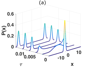
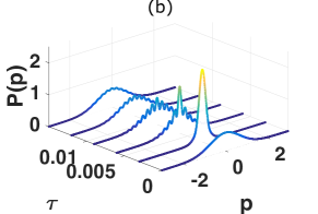
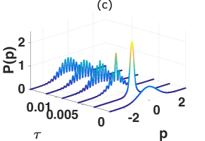
Figure 1: Effect of squeezed reservoirs on the cat state formation in a highly nonlinear DPO without Kerr nonlinearity, at zero temperature. The top plot (a) shows the $x$-quadrature probability distribution as a function of time $\tau$. The case without squeezing ($N_{s}=0$) and with squeezing ($N_{s}=1$, $M=\sqrt{2}$) share similar time evolution of the $x$-quadrature probability distribution. The lower plots [(b) and (b)] show the $p$-quadrature probability distribution (b) without squeezing $N_{s}=0$, and (c) with squeezing $N_{s}=1$. The parameters are $g=2.5$, $\alpha_{0}=\lambda/g^{2}=100$, $N_{th}=0$ and $M=\sqrt{N_{s}\left(N_{s}+1\right)}$.

Fig. 1 shows the time evolution of the $p$-quadrature probability distribution at zero temperature with and without a squeezed input. We see that interference fringes start to appear after $\tau=0.005$. However, for a squeezed input, the interference fringes are more refined. The visibility of the interference fringes is significantly higher than the fringes without a squeezed reservoir at the same dimensionless time $\tau$. In Fig. 1, we see that the $x$-quadrature probability distribution for the cases with and without squeezing are similar. For real $\alpha_{0}$, the existence of two peaks in the $x$-quadrature in Fig. 1 implies well-separated coherent state amplitudes, while the interference fringes in the corresponding $p$-quadrature in Fig. 1 are an indication of the quantum nature of the underlying state. These fringes rule out the possibility of the state being in a classical mixture of two coherent states with amplitudes $\pm\alpha_{0}$. Clearly, from the Figures, a squeezed input enhances the lifetime of the cat state.

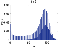
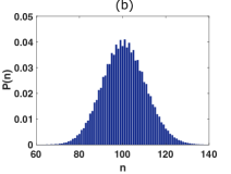
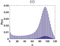
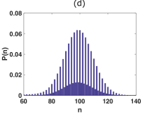
Figure 2: The effect of squeezed reservoirs on the cat-state formation as shown by the photon number distribution. Plots show the photon number probability distribution at times $\tau=0.0075$ [(a) and (c)] and the later time $\tau=0.015$ [(b) and (d)]. The parameters are $g=2.5$, $\lambda/g^{2}=100$, $N_{th}=0$ and $M=\sqrt{N_{s}\left(N_{s}+1\right)}$. Figs. (a) and (b) (top) correspond to a reservoir with no squeezing. Figs. (c) and (d) (lower) correspond to a squeezed reservoir ($N_{s}=1$, $M=\sqrt{2}$), where we see that the probability for an odd photon number is highly suppressed.

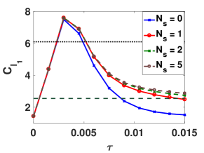
Figure 3: The time evolution of $C_{l_{1}}$ at zero temperature ($N_{th}=0$) for different squeezing strengths. Parameters are $g=2.5$, $\lambda/g^{2}=100$, $\chi=0$, and $M=\sqrt{N_{s}\left(N_{s}+1\right)}$. The upper dashed horizontal line gives the value for a pure cat state eq. (7), and the lower horizontal line gives the value for a mixture (10).

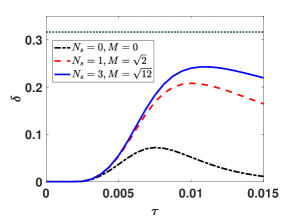
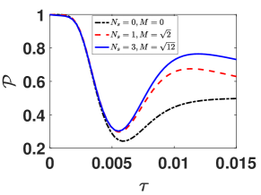
Figure 4: The effect of squeezed reservoirs on the cat-state formation as shown by negativity and purity. The plots give the Wigner negativity $\delta$ and purity $\mathcal{P}$ as a function of the dimensionless time $\tau$, for different degrees of squeezing, at zero temperature $N_{th}=0$. $N_{s}$ is the mean photon number of the squeezed state and $M=\sqrt{N_{s}\left(N_{s}+1\right)}$ determines the strength of squeezing. Parameters are $g=2.5$ and $\lambda/g^{2}=100$. The upper dashed horizontal line in the top figure gives the negativity value for a pure cat state eq. (7). The mixture (10) has zero negativity.

According to Kennedy and Walls (Kennedy and Walls, 1988), the single photon loss can be totally suppressed if the condition $\text{ln}N_{s}\gg 2\tau_{int}$ is satisfied, where $\tau_{int}$ is the dimensionless time of interest before measuring the state of the system. We note that this is only true for the zero temperature case. In practice, the energy required to achieve the amount of squeezing does not scale favorably with the number, $N_{s}$. For instance, from Eq. (4), we see that the $p$-quadrature is squeezed and a squeezing of $82.84\%$ is needed for $N_{s}=1$ while a squeezing of $89.90\%$ is needed for $N_{s}=2$. Hence, the amount of squeezing shown in Figure 1 is $N_{s}=1$ corresponding to $\Delta^{2}P=0.17\Delta^{2}P_{\text{vac}}$, where $\Delta^{2}P_{\text{vac}}=1$ is the variance of the $p$-quadrature for a vacuum state.

The photon number distribution provides a clear perspective on why the interference fringes have higher visibility for a squeezed input. By comparing the photon number distribution at $\tau=0.0075$ and $0.0150$ with squeezing in Fig. 2(b, d) and without squeezing in Fig. 2(a, c), we see that the probability for an odd number is suppressed in the presence of a squeezed reservoir. In other words, the system retains a high probability to be in an even cat-state for a longer time, as compared to the case without the squeezed reservoir. The photon number distribution results suggest that the effect of the squeezing is to maintain the purity of the state for longer times. We quantify this by evaluating the quantum coherence, negativity and purity, in Figures 3 and 4. The quantum coherence and Wigner negativity signatures are improved with the increase of squeezing in the reservoir.

The results for purity as in Eq. (19) are plotted in Fig. 4. Larger squeezing in the input reservoir leads to higher purity, at a given time. We note the dip in the purity during the time evolution before increasing again. This is also observed in the case where the initial and final states are pure states, implying that the state during evolution is not generally a pure one (Hach III and Gerry, 1994). Eventually, for long times, the purity approaches $50\%$, as the cat state becomes a nearly equal mixture of two coherent states.

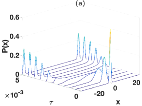
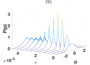
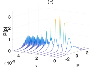
Figure 5: Formation of a large cat state in a DPO at zero temperature with the aid of squeezing. The time evolution of the $x$ and $p$-quadratures without a squeezed reservoir are shown in Plots (a) and (b). The time evolution with a squeezed reservoir $N_{s}=2$, $M_{s}=\sqrt{6}$ is shown (c). The plot for the $x$-quadrature is indistinguishable from plot (a), with no squeezing. The parameters are $g=2$ and $\lambda/g^{2}=400$ which corresponds to a coherent amplitude of $\alpha_{0}=20$.

IV.2 Large cat amplitudes

The results presented so far suggest that a fragile mesoscopic/macroscopic quantum state could well be preserved under the influence of a squeezed reservoir. In the following, we consider a large cat-like state with an amplitude $|\alpha_{0}|=20$, which corresponds to a photon number of $400$, and investigate its quantum features. Again, we take the vacuum state as an initial state. The results for the time evolution of the $p$-quadrature probability distributions for a large amplitude $\alpha_{0}=20$, for zero temperature and $\chi=0$, are shown in Fig. 5. We compare the results without squeezing and with significant squeezing $(N=2,\,M=\sqrt{6},$ $\Delta^{2}p=0.1\Delta^{2}p_{\text{vac}}$). In accordance with the earlier results for a smaller coherent amplitude in Fig. 1, we see an enhancement of the interference fringes in the $p$-quadrature probability distribution when the reservoir is squeezed. Different to the case of no squeezing, the interference fringes persist to the end of our simulation at dimensionless time $\tau=0.0050$.

V cat-states for microwave fields with squeezed-state reservoirs

We now include the thermal contribution and compare cases with and without a squeezed reservoir. While thermal noise at room temperature for optical fields is negligible, the effect of such noise is significant if present. This helps us to understand the results for the microwave regime, where thermal noise will be significant at room temperature. For concreteness, we calculate the mean thermal photon number at room temperature for the signal mode using the experimental parameters of Leghtas et al. (Leghtas et al., 2015). The signal mode frequency is taken to be half the pump mode frequency, which is $\omega_{s}=2\pi\times 4.01\text{GHz}$. The mean thermal number is then given by the expression $N_{th}=1/\left[\text{exp}\left(\hbar\omega_{s}/kT\right)-1\right]\approx 1522$. At cryogenic temperatures of $T\sim 100mK$, $N_{th}$ is of course much lower, and therefore values of $N_{th}=.05-1$ are more typical of these experiments, but thermal effects can still be very significant.

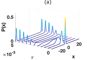
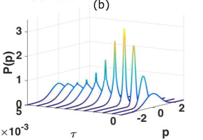
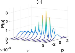
Figure 6: Effect of thermal noise. The time evolution the $x$-quadrature without squeezing ($N_{s}=M=0$) is given by the top graph (a), and is unchanged for squeezing given by $N_{s}=2$, $M=\sqrt{6}$. The middle graph (b) shows the $p$-quadrature without squeezing, and the lower graph (c) shows the $p$-quadrature with squeezing $N_{s}=2$, $M=\sqrt{6}$. Here $N_{th}=0.5$. The parameters are as for Figure 5.

In the Appendix, we summarize results based on the solutions of Kennedy and Walls (Kennedy and Walls, 1988), analyzing the decoherence of a system initially in a cat state, which is then coupled to a thermal squeezed reservoir. We consider both types of thermal squeezing. Without squeezing, thermal noise increases the decoherence rate, and the decoherence rate increases with the size $\alpha$ of the cat state. With squeezing, the decoherence is slowed. However, for a reservoir in a thermalized squeezed state, one cannot overcome the decoherence for finite $N_{th}$ by simply increasing the amount of squeezing. A different result is obtained for the squeezed thermal input, where enhanced squeezing will eventually reduce the decoherence. This is expected, since in the latter, the thermal noise is from the preparation of the squeezed state, and does not arise from the immediate environment of the cavity.

V.1 Thermal effects on cat-states

First, we examine the case of a thermalized squeezed reservoir, which models a system where the environment is at finite temperature as the cat states evolve, but assuming the squeezed input is generated at zero temperature. Results for the quadrature probability distributions and the photon number probability distributions are shown in Figures 6 and 7 respectively. Even for $N_{th}\sim 0.5-1$, thermal noise has a dramatic effect in enhancing the ratio of odd to even photon numbers, thus reducing the purity. In the presence of thermal noise, the squeezing parameters that allow significant improvement of the fringe visibility at zero temperature are no longer sufficient to suppress the loss of quantum coherence. The plots in Figure 8 indicate that the effect of thermal noise is not overcome by simply introducing a large amount of squeezing, as consistent with the results given in the Appendix. More optimistic results would be expected for the squeezed thermal input.

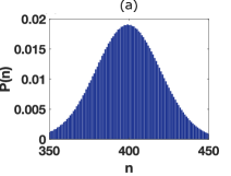
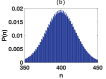
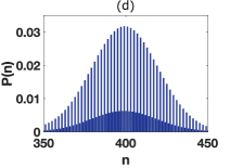
Figure 7: Effect of thermal noise. The photon number probability distribution at $\tau=0.0050$ for the case (a) without squeezing ($N=2,\,M=0$) and (b) with squeezing ($N_{s}=2,\,M=\sqrt{6}$), at a finite temperature, $N_{th}=0.5$. The non-Poissonian character is significantly reduced compared to the case with zero temperature $N_{th}=0$, plotted directly below, for the same squeezing parameters $N_{s}=0$ (c) and $N_{s}=2,$$M=\sqrt{6}$ (d).

Figure 8: The time evolution of $C_{l_{1}}$ at a finite temperature corresponding to $N_{th}=1$, for different squeezing strengths. Parameters are $g=2.5$, $\lambda/g^{2}=100$, $\chi=5$, and $M=\sqrt{N_{s}\left(N_{s}+1\right)}$, as in Fig. 11. The upper dashed horizontal line gives the value for a pure cat state eq. (7), and the lower horizontal line gives the value for a mixture (10).

V.2 Effects of Kerr nonlinearities

Next, we extend the study to a superconducting circuit experiment where Kerr nonlinearity, represented by $\bar{\chi}$ in equation (1), is present. Typically, thermal noise is not negligible. As shown in previous work, (Sun et al., 2019a, b; Teh et al., 2020), the Kerr nonlinearity rotates the steady state about the origin in phase space. We will see that thermal noise induces decoherence and shortens the cat-state lifetime.

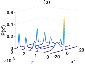
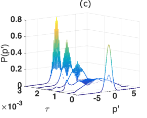
Figure 9: Formation of cat states using squeezed reservoirs for the microwave system. The $x^{\prime}$-quadrature probability distribution and $p^{\prime}$-quadrature probability distribution are plotted as a function of dimensionless time $\tau$, assuming zero temperature $N_{th}=0$ and with Kerr nonlinearity $\chi=5$. The parameters are $g=2.5$, $\lambda/g^{2}=100$. The amount of squeezing is determined by $M=\sqrt{N_{s}\left(N_{s}+1\right)}$. Plot (b) is for $N_{s}=0$ (no squeezing). Plot (c) is for $N_{s}=2$, $M=\sqrt{6}$ (squeezing is present). The $x^{\prime}$-quadrature graphs (a) are indistinguishable for each case.

In the presence of Kerr nonlinearity, the steady state of the system in the limit of zero signal damping and for an initial vacuum state corresponds to a cat state with complex amplitude $\alpha_{0}=\pm\sqrt{\lambda/\left(g^{2}+i\chi^{\prime}\right)}$ (Sun et al., 2019b). The interference fringes in this case are observed along the $P_{\theta}$ quadrature, where $\theta$ is the phase angle of the complex number $\alpha_{0}=|\alpha_{0}|\text{e}^{i\theta}$. It is therefore desirable to have the reservoir in a squeezed state along the direction of the $P_{\theta}$ quadrature. This can be achieved by choosing $M=|M|\text{e}^{2i\theta}$, as can be seen in Eq. (4), with $|M|=\sqrt{N_{s}\left(N_{s}+1\right)}$ giving the optimal squeezing strength.

To study the effect of the squeezed reservoir, we first consider the zero temperature case. In Fig. 9, we observe two Gaussian peaks along the direction of the $x^{\prime}$-quadrature, indicating the formation of two coherent amplitudes with opposite phases. As previously mentioned, the quantum nature of the state is inferred from the $p^{\prime}$-quadrature probability distribution. Fig. 9 shows interference fringes. The visibility of these fringes is higher with squeezing $N_{s}=2$. This is confirmed by the time evolution of the Wigner negativity as presented in Fig. 10. We see that the Wigner negativity is larger for $N_{s}=2$ as compared to $N_{s}=0$, after the two peaks have formed along the $x^{\prime}$-quadrature around $\tau=0.002$. The corresponding purity is also higher with squeezing.

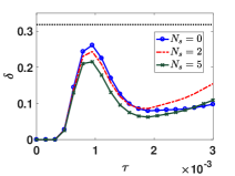
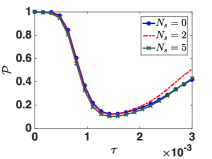
Figure 10: The time evolution of the Wigner negativity (left) and purity (right) at zero temperature ($N_{th}=0$) and for $\chi=5$, for different squeezing strengths. Here, the parameters are $g=2.5$, $\lambda/g^{2}=100$ and $M=\sqrt{N_{s}\left(N_{s}+1\right)}$. The negativity value corresponding to the pure cat state eq. (7) is $\delta=0.318$ as shown in Figure 4. The mixture (10) has zero negativity.

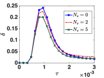
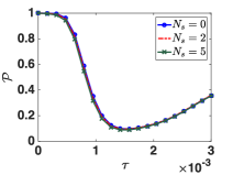
Figure 11: The time evolution of the Wigner negativity (left) and purity (right) at a finite temperature corresponding to $N_{th}=1$, for different squeezing strengths. Parameters are $g=2.5$, $\lambda/g^{2}=100$, $\chi=5$, and $M=\sqrt{N_{s}\left(N_{s}+1\right)}$.

However, the same figure shows a lower Wigner negativity and purity for a larger squeezing strength $N_{s}=5$, compared to that with $N_{s}=2$. These results can be understood by realizing that throughout the simulation, the reservoir squeezing is along the $p^{\prime}$-quadrature and anti-squeezed along the $x^{\prime}$-quadrature, while the steady-state of the system only reaches two coherent amplitudes with opposite phases along the $x^{\prime}$-quadrature after a certain time. In other words, before the system reaches the steady-state the squeezed reservoir adds noise with a non-optimal orientation . This is evident from the slightly counter-intuitive result of lower Wigner negativities for larger squeezing amplitudes, as shown in Fig. 10, before the development of the two probability distribution peaks along the $x^{\prime}$-quadrature. In the case of finite temperature, the thermal bath contributes further extra noise to the system. This is shown in Fig. 11, where the application of the squeezed state with fixed direction has little effect on the negativity.

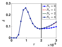
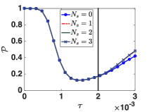
Figure 12: The time evolution of the Wigner negativity (left) and purity (right) at zero temperature, for different squeezing strengths. Here, different to Fig. 10, the squeezed reservoir only interacts with the system at the time of formation of the two distinct peaks along the $x^{\prime}$-quadrature. The vertical line at $\tau=0.002$ is the time when the squeezed state is applied.

To overcome this effect, we can take two approaches. First we allow the system to evolve without squeezing of reservoirs until near the time for the two distinct peaks in $x^{\prime}$ to form. For the parameters of Figure 10, this corresponds to $\tau\sim 0.002$. At that time, we include a squeezed reservoir, the direction of squeezing being in the $p^{\prime}$ direction. This models the insertion of a squeezed state into the input port of a single-ended cavity. The results of the simulation are shown in Fig. 12, where it is seen that the squeezing gives an increased value of the negativity after that time. The second approach is to apply a squeezed state that has a varying direction, to match at a given time the direction $p^{\prime}$ orthogonal to the rotating amplitudes $\alpha_{0}$.

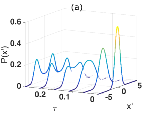
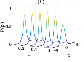
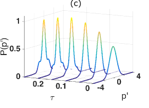
Figure 13: The $x^{\prime}$-quadrature (a) and $p^{\prime}$-quadrature [(b) and (c)] probability distributions as a function of dimensionless time $\tau$, at a finite temperature $N_{th}=0.02$. Here, the coherent amplitude is $|\alpha_{0}|=2$. The parameters are $g=1.41$ and $\chi^{\prime}=1.01$, which are taken from the experiment of Leghtas et al. (Leghtas et al., 2015). Plot (b) is without squeezing, $N_{s}=0$. Plot (c) is with squeezing $N_{s}=0.5$. The $x^{\prime}$-quadrature probability distributions with and without squeezing are indistinguishable.

V.3 Squeezing effects with typical experimental parameters

Next, we look at the effects of a squeezed reservoir using experimental parameters for the superconducting circuit experiment of Leghtas et al. (Leghtas et al., 2015). Here we evaluate $g=1.41$ and $\chi^{\prime}=1.01$, giving an estimated $\chi=\chi^{\prime}/g^{2}=0.5$ and $|\alpha_{0}|=2$. The mean thermal photon number is very low, at $N_{th}\leq 0.05\ll 1$, which is set here at $N_{th}=0.02$. We present the $x^{\prime}$-quadrature probability distributions in Fig. 13 and observe that the two peaks along $x^{\prime}$ do not become that well separated. The simulation introduces the squeezed reservoir after $\tau=0.1$, when the two peaks are starting to develop.

The effect of adding a squeezed reservoir, which was not present in the original experiment, can be observed in Fig. 13 where we show the time evolution of the $p^{\prime}$-quadrature probability distribution. Without the squeezed reservoir, the $p^{\prime}$-quadrature probability distribution is Gaussian-like throughout the simulation. The probability distribution with squeezing displays some features of interference fringes, suggesting a quantum state with larger non-classicality in the presence of the squeezed reservoir. This is confirmed in Fig. 14 where we compare the Wigner negativity and purity for the case without and with squeezing. With squeezing, the Wigner negativity has a larger value. Similarly, there is an increase in the purity of the quantum state.

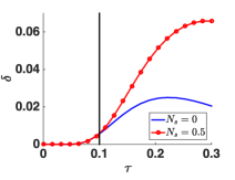
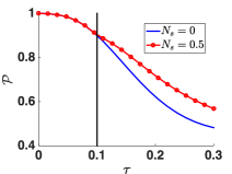
Figure 14: The time evolution of (left) the Wigner negativity and (right) purity. The parameters are identical to those given in Figs. 13.

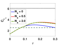
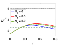
Figure 15: The time evolution of quantum coherence $C_{l_{1}}$ for the evolution of a cat-like state using parameters similar to the experiment of Ref (Leghtas et al., 2015). For each plot we show results with squeezing (upper red solid line) and without squeezing (lower blue solid line). The results for parameters similar to the experiment ($g=1.41$, $N_{th}=0.02$, $\chi^{\prime}=1.01$) are shown in the figure on the right. Parameters for the left figure are $g=1.41$, $N_{th}=0$, $\chi^{\prime}=0$, and are given for comparison. In both figures, $|\alpha_{0}|=2$ and $M=\sqrt{N_{s}\left(N_{s}+1\right)}$ when $N_{s}\neq 0$. The upper horizontal dashed line gives the $C_{l_{1}}$ value of the corresponding cat state. The lower dashed horizontal line gives the $C_{l_{1}}$ value for mixture of coherent states with amplitude $|\alpha_{0}|=2$.

To probe the properties of the cat-like state that might be generated in a potential experiment, we next calculate the quantum coherence $C_{l_{1}}(\rho)$ for the transient cat-like states versus time. For the purpose of comparison, Figure (8) gives the values of $C_{l_{1}}(\rho)$ for the pure cat state and for the mixture $\rho_{mix}$ of the two coherent states. As explained in Section III, the quantum coherence for the mixture arises from the quantum coherence of the coherent states $|\pm\alpha\rangle$ involved in the mixture, whereas the quantum coherence for the cat state contains the extra contribution due to the state being a macroscopic superposition. Figure 15 gives the $C_{l_{1}}(\rho)$ for the parameters of the Leghtas et al experiment. Here, the quantum coherence is at 50% the value for an ideal cat state, significantly above that of the mixture, and it can be seen that the squeezing enhances the lifetime for a higher quantum coherence. When squeezing is present, the $C_{l_{1}}$ values are higher, implying a higher degree of quantum coherence. However, consistent with the observation that the threshold features for the cat state cannot be significantly altered by squeezing, we note that the effect of squeezing saturates, in this case at $N_{s}\sim 0.5$. Using the experimental parameters of Leghtas et al. (Leghtas et al., 2015), where the signal mode frequency is $\omega_{s}=2\pi\times 4.01\text{GHz}$, and the expression $N_{th}=1/\left[\text{exp}\left(\hbar\omega_{s}/kT\right)-1\right]$, a mean thermal photon number $N_{th}$ of $0.02$ corresponds to a temperature $T\approx 50\text{mK}$.

VI Conclusion

In this paper, we have demonstrated the feasibility of using quantum squeezed states to enhance the macroscopic quantum coherence of dynamical cat states prepared in a cavity through a nonlinear parametric interaction. Here, we have focussed on degenerate parametric oscillation (DPO) in the limit of an adiabatically eliminated pump mode, where a two-photon dissipative mechanism dominates. The cat state, which is a superposition of two coherent states with a $\pi$ phase difference, is predicted to be created in the cavity signal mode from an initial vacuum state, in the limit where there are no losses in the cavity mode. A cat state is also predicted in the microwave regime, where extra nonlinear terms are present. The loss of photons from the cavity decoheres the cat state. Thus, whether the cat state is formed or not depends on the dynamical interplay of the quantum nonlinear effect versus the signal decoherence.

We have found that it is possible to significantly limit the effects of decoherence, by squeezing the input vacuum noise that enters the cavity port at the signal frequency. This amounts to controlling the fluctuations of the reservoir. The cat state then has a longer lifetime, which enables the formation of cat states of a higher purity for the same experimental parameters. Our result is consistent with earlier work on the decoherence of a pure cat state, and extends previous treatments of the effect of squeezing on cat states formed in the DPO system by giving a broader range of parameters and implementing different signatures, such as negativity and measures of quantum coherence.

We obtain new results for the microwave system, which is relevant to current experiments, and based on a different Hamiltonian. We find that the direction of squeezing is important. The enhancement occurs when the quantum noise of the signal cavity input is squeezed in the direction orthogonal to the axis connecting the amplitudes of the two coherent states. This rotates with the dynamics, and hence the squeezing direction needs to be controlled. Ultimately, the direction is determined by the type of nonlinearity, and whether an additional Kerr effect is present.

Thermal noise also induces a decoherence of the cat state and has a profound effect on the feasibility of creating the cat states in the dynamical system. In the microwave regime, cooling is necessary to observe the formation of cat states. We have shown how the presence of squeezing enhances the quality of the cat state that can be formed for systems at a temperature corresponding to the microwave experiment of Leghtas et al (Leghtas et al., 2015). Our results are based on statistics modeled on a squeezed thermalized reservoir, and are consistent with earlier treatments (Kennedy and Walls, 1988; Serafini et al., 2005, 2004b), showing that while squeezing can inhibit the thermal decoherence, the thermal decoherence cannot be completely overcome by further increasing squeezing. This contrasts with the result in the absence of thermal noise. On the whole, based on analytical calculations where one analyses the decoherence of an ideal cat state coupled to a reservoir, we anticipate a more promising situation for a squeezed thermal state input. This models a squeezed state generated from a source at nonzero temperature, but requires that the cavity be kept at zero temperature over the timescales during which the cat state forms in the cavity.

Appendix

1. Statistical moments for a squeezed thermal state

A squeezed thermal state has a corresponding density operator (Fearn and Collett, 1988; Kim et al., 1989)

$$\rho_{ST} =S\rho_{T}S^{\dagger}$$

$$=\frac{1}{1+N_{th}}\sum_{n}\left(\frac{N_{th}}{1+N_{th}}\right)^{n}S|n\rangle\langle n|S^{\dagger}\,,$$

where $S(\epsilon)=\text{exp}\left[\left(\epsilon^{*}\Gamma^{2}-\epsilon\Gamma^{\dagger 2}\right)/2\right]$ is the squeezing operator, $\epsilon=re^{i\phi}$ and $N_{th}$ is the mean photon number of a thermal state. The mean photon number for the squeezed thermal state is

$$\langle\Gamma^{\dagger}\Gamma\rangle =N_{th}\cosh 2r+\sinh^{2}r\,,$$

while other statistical moments are given by

$$\langle\Gamma^{2}\rangle =-\frac{1}{2}\sinh 2re^{i\phi}\left(2N_{th}+1\right)$$

and

$$\langle\Gamma^{\dagger 2}\rangle =-\frac{1}{2}\sinh 2re^{-i\phi}\left(2N_{th}+1\right)\,.$$

Compare these equations with the statistical moments for the environment mode operators in Eq. (2), we see that, for a squeezed thermal state,

$$N =N_{th}\cosh 2r+\sinh^{2}r$$

$$M =-\frac{1}{2}\sinh 2re^{i\phi}\left(2N_{th}+1\right)$$

$$=\frac{1}{2}\left(2N_{th}+1\right)\sinh 2re^{i\left(\phi-\pi\right)}\,.$$

In particular, for $\theta=0$, the variances of $X$ and $P$ quadratures as defined in Eq. (3) have the expressions:

$$\Delta^{2}X =\left(N_{th}\cosh 2r+\sinh^{2}r+\frac{1}{2}\right)$$

$$+\frac{1}{2}\sinh 2r\left(2N_{th}+1\right)\cos\left(\phi-\pi\right)$$

$$\Delta^{2}P =\left(N_{th}\cosh 2r+\sinh^{2}r+\frac{1}{2}\right)$$

$$-\frac{1}{2}\sinh 2r\left(2N_{th}+1\right)\cos\left(\phi-\pi\right)\,.$$ (20)

In order to get a squeezing in the $P$ quadrature, we set $\phi=\pi$ ($M$ is real with amplitude $\left(N_{th}+1/2\right)\sinh 2r$) and Eq. (20) is then

$$\Delta^{2}X =\left(N_{th}+\frac{1}{2}\right)e^{2r}$$

$$\Delta^{2}P =\left(N_{th}+\frac{1}{2}\right)e^{-2r}\,.$$ (21)

We note that the thermal contribution is squeezed (anti-squeezed) by the factor of $e^{-2r}$ ($e^{2r}$). This means that such thermal squeezing (if in the direction so as to squeeze fluctuations in $P$) would give significant enhancement of the observed macroscopic quantum coherence. We do not give explicit calculation of such enhancement in this paper, but the calculations could be done in principle by substituting for $N$ and $M$.

2. Statistical moments for a thermalized squeezed state

Fearn and Collett (Fearn and Collett, 1988) defined a thermalized squeezed state with a density operator in the coherent basis (Glauber-P representation) as follows:

$$\rho_{TS} =\frac{1}{\pi N_{th}}\intop d^{2}\beta\,\text{exp}\left(-\frac{\left|\beta\right|^{2}}{N_{th}}\right)|\beta,\epsilon\rangle\langle\beta,\epsilon|\,,$$

where $|\beta,\epsilon\rangle=D(\beta)S(\epsilon)|0\rangle=S(\epsilon)D(\gamma)|0\rangle$ is a displaced squeezed state, $D(\beta)$ is the displacement operator, $S(\epsilon)$ is the squeezing operator as defined in the previous section and $\gamma=\beta\cosh r+\beta^{*}e^{i\phi}\sinh r$.

The mean photon number for the thermalized squeezed state is

$$\langle\Gamma^{\dagger}\Gamma\rangle =\sinh^{2}r+N_{th}$$

and the statistical moments $\langle\Gamma^{2}\rangle$ and $\langle\Gamma^{\dagger 2}\rangle$ are

$$\langle\Gamma^{2}\rangle =\frac{1}{2}\sinh 2re^{i\left(\phi-\pi\right)}$$

$$\langle\Gamma^{\dagger 2}\rangle =\frac{1}{2}\sinh 2re^{-i\left(\phi-\pi\right)}\,.$$

Comparing these equations with the statistical moments for the environment mode operators in Eq. (2), we see that, for a thermalized squeezed state

$$N =N_{th}+\sinh^{2}r$$

$$M =\frac{1}{2}\sinh 2re^{i\left(\phi-\pi\right)}\,.$$ (22)

For $\theta=0$ and $\phi=\pi$, the variances of $X$ and $P$ quadratures as defined in Eq. (3) have the expressions:

$$\Delta^{2}X =2N_{th}+e^{2r}$$

$$\Delta^{2}P =2N_{th}+e^{-2r}\,.$$ (23)

As opposed to the squeezed thermal state, the thermal number $N_{th}$ in Eq. (23) is not affected by the squeezing operation, implying that the squeezing is weaker for a thermalized squeezed state with the same squeezing strength $r$ as in the squeezed thermal state.

3. Effect of thermal noise on decoherence of a system prepared initially in a cat state

Kennedy and Walls (Kennedy and Walls, 1988) investigated the effect of squeezing on the probability distribution interference fringes visibility. They considered an initial cat state with a density operator $\rho(0)=\mathcal{N}\left(e^{-i\pi/4}|\alpha\rangle+e^{i\pi/4}|-\alpha\rangle\right)\left(e^{i\pi/4}\langle\alpha|+e^{-i\pi/4}\langle-\alpha|\right)$. The term in the probability distribution for $x_{\theta}$ that contributes to the interference fringes is found to be proportional to $\left|\langle\alpha|-\alpha\rangle\right|^{\eta}$:

$$\langle x_{\theta}|\rho(t)|x_{\theta}\rangle \propto\left|\langle\alpha|-\alpha\rangle\right|^{\eta}$$

$$=\exp\left(-2|\alpha|^{\eta}\right)\,$$ (24)

where

$$\eta =1-\frac{e^{-2\gamma t}}{\left\{1+2\left[N+|M|\cos\left(2\theta+\Phi\right)\right]\left(1-e^{-2\gamma t}\right)\right\}}\,,$$

$\theta$ determines the phase quadrature $x_{\theta}$, and $\Phi$ is the phase of the complex parameter $M$, as previously defined. Here, $N=N_{th}+N_{s}$. For the cat state considered, it is optimal to choose $\cos\left(2\theta+\phi\right)=-1$.

Figure 16: The term that contributes to the interference pattern $\eta$ as a function of $\gamma t$. $\eta=0$ demonstrates full visibility of the interference fringes. The visibility is zero when $\eta=1$. This figure corresponds to a system with zero temperature. Squeezing increases with $r$, the squeeze parameter.

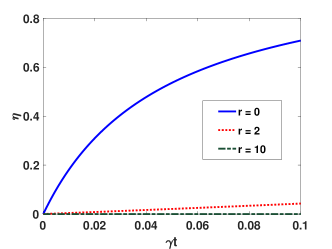
Figure 17: Here, $\eta=0$ demonstrates full visibility of interference fringes. The visibility is zero when $\eta=1$. This figure corresponds to a squeezed thermal state at a finite temperature with $N_{th}=5$.

Figure 18: Here, $\eta=0$ demonstrates full visibility of interference fringes. The visibility is zero when $\eta=1$. This figure corresponds to a thermalized squeezed state at a finite temperature with $N_{th}=5$.

We now summarize the results for the two types of thermal states considered above. We examine results for the type of squeezing that comes from a DPO, denoting the squeezing parameter by $r$, and where $M=\sqrt{N_{s}\left(N_{s}+1\right)}$. For a thermalized squeezed bath, $N=N_{th}+\sinh^{2}r=N_{th}+N_{s}$, $r$ is the squeezing strength and $\left|M\right|=\frac{1}{2}\sinh 2r$ as calculated in the above. For a squeezed thermal bath, $N=N_{th}\cosh 2r+\sinh^{2}r$ and $\left|M\right|=\frac{1}{2}\left(2N_{th}+1\right)\sinh 2r$. Figure 16 shows the decoherence where there is damping but no thermal noise, so that $N_{th}=0$. In this limit, the decoherence can be totally suppressed for longer times for sufficiently strong squeezing, where $N_{s}\rightarrow\infty$.

The results for a squeezed thermal state are given in Figure 18. Here, we see on comparing (21) with (23) that the effect on the squeezing variances is such that the effect of the thermal noise term $N_{th}$ for the squeezed thermal state is itself reduced by increasing squeezing parameter. This arises because the technique of preparation is to reduce, or squeeze, the thermal noise at the squeezing source. From the figure, we see that with a sufficient amount of squeezing it is possible to completely suppress the decoherence due to thermal noise for this type of squeezed thermal input.

Looking at the thermalized squeezed state, we find for finite $N_{th}$ and infinite squeezing

$$\eta \rightarrow 1-\frac{e^{-2\gamma t}}{\left\{1+2N_{th}\left(1-e^{-2\gamma t}\right)\right\}}$$ (25)

For long times, $\eta\rightarrow 1-\frac{e^{-2\gamma t}}{\left\{1+2N_{th}\right\}}$. This shows that thermal noise (where $N_{th}$ is fixed) remains significant in increasing decoherence. For short times, we obtain a linear response of $\eta$ with $\gamma t$, $\eta\sim 4N_{th}\gamma t$. These features are observed in Figure 17. Consistent with results reported by Serafini et al (Serafini et al., 2004b, 2005, a), we also note that increasing squeezing does not always lead to a decrease of decoherence over a certain time.

References

- Schrödinger (1935) E. Schrödinger, Naturwissenschaften 23, 823 (1935).
- Brune et al. (1996) M. Brune, E. Hagley, J. Dreyer, X. Maître, A. Maali, C. Wunderlich, J. M. Raimond, and S. Haroche, Physical Review Letters 77, 4887 (1996).
- Monroe et al. (1996) C. Monroe, D. M. Meekhof, B. E. King, and D. J. Wineland, Science 272, 1131 (1996).
- Friedman et al. (2000) J. R. Friedman, V. Patel, W. Chen, S. K. Tolpygo, and J. E. Lukens, Nature 406, 43 (2000).
- Ourjoumtsev et al. (2007) A. Ourjoumtsev, H. Jeong, R. Tualle-Brouri, and P. Grangier, Nature 448, 784 EP (2007).
- Palacios-Laloy et al. (2010) A. Palacios-Laloy, F. Mallet, F. Nguyen, P. Bertet, D. Vion, D. Esteve, and A. N. Korotkov, Nature Physics 6, 442 EP (2010).
- Vlastakis et al. (2013) B. Vlastakis, G. Kirchmair, Z. Leghtas, S. E. Nigg, L. Frunzio, S. M. Girvin, M. Mirrahimi, M. H. Devoret, and R. J. Schoelkopf, Science 342, 607 (2013).
- Wang et al. (2016) C. Wang, Y. Y. Gao, P. Reinhold, R. W. Heeres, N. Ofek, K. Chou, C. Axline, M. Reagor, J. Blumoff, K. M. Sliwa, L. Frunzio, S. M. Girvin, L. Jiang, M. Mirrahimi, M. H. Devoret, and R. J. Schoelkopf, Science 352, 1087 (2016).
- Yurke and Stoler (1986) B. Yurke and D. Stoler, Physical Review Letters 57, 13 (1986).
- Knee et al. (2016) G. C. Knee, K. Kakuyanagi, M.-C. Yeh, Y. Matsuzaki, H. Toida, H. Yamaguchi, S. Saito, A. J. Leggett, and W. J. Munro, Nature Communications 7, 1 (2016).
- Leggett and Garg (1985) A. J. Leggett and A. Garg, Physical Review Letters 54, 857 (1985).
- Marshall et al. (2003) W. Marshall, C. Simon, R. Penrose, and D. Bouwmeester, Physical Review Letters 91, 130401 (2003).
- Vanner et al. (2011) M. R. Vanner, I. Pikovski, G. D. Cole, M. Kim, Č. Brukner, K. Hammerer, G. J. Milburn, and M. Aspelmeyer, Proceedings of the National Academy of Sciences 108, 16182 (2011).
- Vanner (2011) M. R. Vanner, Physical Review X 1, 021011 (2011).
- Asadian et al. (2014) A. Asadian, C. Brukner, and P. Rabl, Physical Review Letters 112, 190402 (2014).
- Teh et al. (2018) R. Y. Teh, S. Kiesewetter, P. D. Drummond, and M. D. Reid, Physical Review A 98, 063814 (2018).
- Budroni et al. (2015) C. Budroni, G. Vitagliano, G. Colangelo, R. J. Sewell, O. Gühne, G. Tóth, and M. W. Mitchell, Physical Review Letters 115, 200403 (2015).
- Opanchuk et al. (2016) B. Opanchuk, L. Rosales-Zárate, R. Y. Teh, and M. D. Reid, Physical Review A 94, 062125 (2016).
- Rosales-Zárate et al. (2018) L. Rosales-Zárate, B. Opanchuk, Q. Y. He, and M. D. Reid, Physical Review A 97, 042114 (2018).
- Thenabadu and Reid (2019) M. Thenabadu and M. D. Reid, Physical Review A 99, 032125 (2019).
- Bassi et al. (2013) A. Bassi, K. Lochan, S. Satin, T. P. Singh, and H. Ulbricht, Rev. Mod. Phys. 85, 471 (2013).
- Caldeira and Leggett (1985) A. O. Caldeira and A. J. Leggett, Physical Review A 31, 1059 (1985).
- Walls and Milburn (1985) D. F. Walls and G. J. Milburn, Physical Review A 31, 2403 (1985).
- Leghtas et al. (2013) Z. Leghtas, G. Kirchmair, B. Vlastakis, M. H. Devoret, R. J. Schoelkopf, and M. Mirrahimi, Physical Review A 87, 042315 (2013).
- Leghtas et al. (2015) Z. Leghtas, S. Touzard, I. M. Pop, A. Kou, B. Vlastakis, A. Petrenko, K. M. Sliwa, A. Narla, S. Shankar, M. J. Hatridge, M. Reagor, L. Frunzio, R. J. Schoelkopf, M. Mirrahimi, and M. H. Devoret, Science 347, 853 (2015).
- Mirrahimi et al. (2014) M. Mirrahimi, Z. Leghtas, V. V. Albert, S. Touzard, R. J. Schoelkopf, L. Jiang, and M. H. Devoret, New Journal of Physics 16, 045014 (2014).
- Wolinsky and Carmichael (1988) M. Wolinsky and H. J. Carmichael, Physical Review Letters 60, 1836 (1988).
- Reid and Yurke (1992) M. D. Reid and B. Yurke, Physical Review A 46, 4131 (1992).
- Hach III and Gerry (1994) E. E. Hach III and C. C. Gerry, Physical Review A 49, 490 (1994).
- Gilles et al. (1994) L. Gilles, B. M. Garraway, and P. L. Knight, Physical Review A 49, 2785 (1994).
- Carmichael and Wolinsky (1986) H. J. Carmichael and M. Wolinsky, in Quantum Optics IV, edited by J. D. Harvey and D. F. Walls (Springer Berlin Heidelberg, Berlin, Heidelberg, 1986) pp. 208–220.
- Kennedy and Walls (1988) T. A. B. Kennedy and D. F. Walls, Physical Review A 37, 152 (1988).
- Haroche (2003) S. Haroche, Philosophical Transactions of the Royal Society of London. Series A: Mathematical, Physical and Engineering Sciences 361, 1339 (2003).
- El-Orany et al. (2003) F. A. El-Orany, J. Peřina, V. Peřinová, and M. S. Abdalla, The European Physical Journal D-Atomic, Molecular, Optical and Plasma Physics 22, 141 (2003).
- Serafini et al. (2004a) A. Serafini, S. De Siena, and F. Illuminati, Modern Physics Letters B 18, 687 (2004a).
- Serafini et al. (2004b) A. Serafini, S. De Siena, F. Illuminati, and M. G. A. Paris, Journal of Optics B: Quantum and Semiclassical Optics 6, S591 (2004b).
- Serafini et al. (2005) A. Serafini, M. G. A. Paris, F. Illuminati, and S. De Siena, Journal of Optics B: Quantum and Semiclassical Optics 7, R19 (2005).
- Paavola et al. (2011) J. Paavola, M. J. Hall, M. G. Paris, and S. Maniscalco, Physical Review A 84, 012121 (2011).
- Rosales-Zárate et al. (2015) L. Rosales-Zárate, R. Y. Teh, S. Kiesewetter, A. Brolis, K. Ng, and M. D. Reid, JOSA B 32, A82 (2015).
- Tan et al. (2014) Q.-S. Tan, J.-Q. Liao, X. Wang, and F. Nori, Physical Review A 89, 053822 (2014).
- Bennett and Bowen (2018) J. S. Bennett and W. P. Bowen, New Journal of Physics 20, 113016 (2018).
- Xiong et al. (2019) B. Xiong, X. Li, S.-L. Chao, Z. Yang, W.-Z. Zhang, and L. Zhou, Optics Express 27, 13547 (2019).
- Yuen (1976) H. P. Yuen, Physical Review A 13, 2226 (1976).
- Caves (1981) C. M. Caves, Physical Review D 23, 1693 (1981).
- Milburn and Walls (1981) G. Milburn and D. Walls, Optics Communications 39, 401 (1981).
- Yurke (1984) B. Yurke, Physical Review A 29, 408 (1984).
- Yurke and Denker (1984) B. Yurke and J. S. Denker, Physical Review A 29, 1419 (1984).
- Collett and Gardiner (1984) M. J. Collett and C. W. Gardiner, Physical Review A 30, 1386 (1984).
- Reid and Walls (1984) M. D. Reid and D. F. Walls, Optics Communications 50, 406 (1984).
- Reid et al. (1985) M. D. Reid, D. F. Walls, and B. J. Dalton, Physical Review Letters 55, 1288 (1985).
- Fabre et al. (1990) C. Fabre, E. Giacobino, A. Heidmann, L. Lugiato, S. Reynaud, M. Vadacchino, and W. Kaige, Quantum Optics: Journal of the European Optical Society Part B 2, 159 (1990).
- Movshovich et al. (1990) R. Movshovich, B. Yurke, P. G. Kaminsky, A. D. Smith, A. H. Silver, R. W. Simon, and M. V. Schneider, Physical Review Letters 65, 1419 (1990).
- Purdy et al. (2013) T. P. Purdy, P.-L. Yu, R. W. Peterson, N. S. Kampel, and C. A. Regal, Physical Review X 3, 031012 (2013).
- Wollman et al. (2015) E. E. Wollman, C. U. Lei, A. J. Weinstein, J. Suh, A. Kronwald, F. Marquardt, A. A. Clerk, and K. C. Schwab, Science 349, 952 (2015).
- Castellanos-Beltran et al. (2008a) M. A. Castellanos-Beltran, K. D. Irwin, G. C. Hilton, L. R. Vale, and K. W. Lehnert, Nature Physics 4, 929 (2008a).
- Slusher et al. (1985) R. E. Slusher, L. W. Hollberg, B. Yurke, J. C. Mertz, and J. F. Valley, Physical Review Letters 55, 2409 (1985).
- Heidmann et al. (1987) A. Heidmann, R. J. Horowicz, S. Reynaud, E. Giacobino, C. Fabre, and G. Camy, Physical Review Letters 59, 2555 (1987).
- Vahlbruch et al. (2008) H. Vahlbruch, M. Mehmet, S. Chelkowski, B. Hage, A. Franzen, N. Lastzka, S. Goßler, K. Danzmann, and R. Schnabel, Physical Review Letters 100, 033602 (2008).
- Mehmet et al. (2011a) M. Mehmet, S. Ast, T. Eberle, S. Steinlechner, H. Vahlbruch, and R. Schnabel, Opt. Express 19, 25763 (2011a).
- Mehmet et al. (2011b) M. Mehmet, S. Ast, T. Eberle, S. Steinlechner, H. Vahlbruch, and R. Schnabel, Optics Express 19, 25763 (2011b).
- Vahlbruch et al. (2016) H. Vahlbruch, M. Mehmet, K. Danzmann, and R. Schnabel, Physical Review Letters 117, 110801 (2016).
- Taylor et al. (2013) M. A. Taylor, J. Janousek, V. Daria, J. Knittel, B. Hage, H.-A. Bachor, and W. P. Bowen, Nature Photonics 7, 229 (2013).
- Toscano et al. (2006) F. Toscano, D. A. R. Dalvit, L. Davidovich, and W. H. Zurek, Physical Review A 73, 023803 (2006).
- Tombesi and Mecozzi (1987) P. Tombesi and A. Mecozzi, J. Opt. Soc. Am. B 4, 1700 (1987).
- Lane et al. (1988) A. S. Lane, M. D. Reid, and D. F. Walls, Physical Review Letters 60, 1940 (1988).
- Gardiner (1986) C. W. Gardiner, Physical Review Letters 56, 1917 (1986).
- Tombesi and Vitali (1994) P. Tombesi and D. Vitali, Physical Review A 50, 4253 (1994).
- Braunstein and Kimble (1998) S. L. Braunstein and H. J. Kimble, Physical Review Letters 80, 869 (1998).
- Mecozzi and Tombesi (1987) A. Mecozzi and P. Tombesi, Physical Review Letters 58, 1055 (1987).
- Munro and Reid (1995) W. J. Munro and M. D. Reid, Physical Review A 52, 2388 (1995).
- Wang et al. (2013) Z. Wang, A. Marandi, K. Wen, R. L. Byer, and Y. Yamamoto, Physical Review A 88, 063853 (2013).
- Marandi et al. (2014) A. Marandi, Z. Wang, K. Takata, R. L. Byer, and Y. Yamamoto, Nature Photonics 8, 937 (2014).
- Shoji et al. (2017) T. Shoji, K. Aihara, and Y. Yamamoto, Physical Review A 96, 053833 (2017).
- Yamamura et al. (2017) A. Yamamura, K. Aihara, and Y. Yamamoto, Physical Review A 96, 053834 (2017).
- McMahon et al. (2016) P. L. McMahon, A. Marandi, Y. Haribara, R. Hamerly, C. Langrock, S. Tamate, T. Inagaki, H. Takesue, S. Utsunomiya, K. Aihara, R. L. Byer, M. M. Fejer, H. Mabuchi, and Y. Yamamoto, Science 354, 614 (2016).
- Inagaki et al. (2016) T. Inagaki, Y. Haribara, K. Igarashi, T. Sonobe, S. Tamate, T. Honjo, A. Marandi, P. L. McMahon, T. Umeki, K. Enbutsu, O. Tadanaga, H. Takenouchi, K. Aihara, K.-i. Kawarabayashi, K. Inoue, S. Utsunomiya, and H. Takesue, Science 354, 603 (2016).
- Nigg et al. (2012) S. E. Nigg, H. Paik, B. Vlastakis, G. Kirchmair, S. Shankar, L. Frunzio, M. H. Devoret, R. J. Schoelkopf, and S. M. Girvin, Physical Review Letters 108, 240502 (2012).
- Goto et al. (2019) H. Goto, Z. Lin, T. Yamamoto, and Y. Nakamura, Physical Review A 99, 023838 (2019).
- Pfaff et al. (2017) W. Pfaff, C. J. Axline, L. D. Burkhart, U. Vool, P. Reinhold, L. Frunzio, L. Jiang, M. H. Devoret, and R. J. Schoelkopf, Nature Physics 13, 882 (2017).
- Goto (2016a) H. Goto, Scientific Reports 6, 21686 (2016a).
- Goto (2016b) H. Goto, Physical Review A 93, 050301 (2016b).
- Puri et al. (2017) S. Puri, C. K. Andersen, A. L. Grimsmo, and A. Blais, Nature Communications 8, 15785 (2017).
- Luo et al. (2020) L. Luo, H. Liu, N. Huang, and Z. Wang, Optics Express 28, 1914 (2020).
- Maruo et al. (2016) D. Maruo, S. Utsunomiya, and Y. Yamamoto, Physica Scripta 91, 083010 (2016).
- Drummond et al. (1981) P. Drummond, K. McNeil, and D. Walls, Optica Acta: International Journal of Optics 28, 211 (1981).
- Krippner et al. (1994) L. Krippner, W. J. Munro, and M. D. Reid, Physical Review A 50, 4330 (1994).
- Sun et al. (2019a) F.-X. Sun, Q. He, Q. Gong, R. Y. Teh, M. D. Reid, and P. D. Drummond, New Journal of Physics 21, 093035 (2019a).
- Sun et al. (2019b) F.-X. Sun, Q. He, Q. Gong, R. Y. Teh, M. D. Reid, and P. D. Drummond, Physical Review A 100, 033827 (2019b).
- Teh et al. (2020) R. Y. Teh, F.-X. Sun, R. E. S. Polkinghorne, Q. Y. He, Q. Gong, P. D. Drummond, and M. D. Reid, Physical Review A 101, 043807 (2020).
- Fearn and Collett (1988) H. Fearn and M. Collett, Journal of Modern Optics 35, 553 (1988).
- Kim et al. (1989) M. S. Kim, F. A. M. de Oliveira, and P. L. Knight, Physical Review A 40, 2494 (1989).
- Gilchrist et al. (1999) A. Gilchrist, P. Deuar, and M. D. Reid, Physical Review A 60, 4259 (1999).
- Fröwis et al. (2018) F. Fröwis, P. Sekatski, W. Dür, N. Gisin, and N. Sangouard, Rev. Mod. Phys. 90, 025004 (2018).
- Kenfack and Zyczkowski (2004) A. Kenfack and K. Zyczkowski, Journal of Optics B: Quantum and Semiclassical Optics 6, 396 (2004).
- Baumgratz et al. (2014) T. Baumgratz, M. Cramer, and M. B. Plenio, Physical Review Letters 113, 140401 (2014).
- Kryuchkyan and Kheruntsyan (1996) G. Kryuchkyan and K. Kheruntsyan, Optics Communications 127, 230 (1996).
- Gardiner and Collett (1985) C. W. Gardiner and M. J. Collett, Physical Review A 31, 3761 (1985).
- Castellanos-Beltran et al. (2008b) M. A. Castellanos-Beltran, K. D. Irwin, G. C. Hilton, L. R. Vale, and K. W. Lehnert, Nature Physics 4, 929 (2008b).
- Ockeloen-Korppi et al. (2017) C. F. Ockeloen-Korppi, E. Damskägg, J.-M. Pirkkalainen, T. T. Heikkilä, F. Massel, and M. A. Sillanpää, Physical Review Letters 118, 103601 (2017).
- Gardiner and Zoller (2004) C. Gardiner and P. Zoller, Quantum Noise: A Handbook of Markovian and Non-Markovian Quantum Stochastic Methods with Applications to Quantum Optics, Springer Series in Synergetics (Springer, 2004).
- Kinsler and Drummond (1991) P. Kinsler and P. D. Drummond, Physical Review A 43, 6194 (1991).
- Terhal and Horodecki (2000) B. M. Terhal and P. Horodecki, Physical Review A 61, 040301(R) (2000).
- Brennen (2003) G. K. Brennen, Quantum Info. Comput. 3, 619 (2003).
- Cavalcanti and Reid (2006) E. G. Cavalcanti and M. D. Reid, Physical Review Letters 97, 170405 (2006).
- Cavalcanti and Reid (2008) E. G. Cavalcanti and M. D. Reid, Physical Review A 77, 062108 (2008).
- Fröwis and Dür (2012) F. Fröwis and W. Dür, New Journal of Physics 14, 093039 (2012).
- Sekatski et al. (2014) P. Sekatski, N. Sangouard, and N. Gisin, Physical Review A 89, 012116 (2014).
- Fröwis et al. (2016) F. Fröwis, P. Sekatski, and W. Dür, Physical Review Letters 116, 090801 (2016).
- Yadin and Vedral (2016) B. Yadin and V. Vedral, Physical Review A 93, 022122 (2016).
- Reid (2019) M. D. Reid, Physical Review A 100, 052118 (2019).
- Cahill and Glauber (1969) K. E. Cahill and R. J. Glauber, Physical Review 177, 1882 (1969).
- Pathak and Banerji (2014) A. Pathak and J. Banerji, Physics Letters A 378, 117 (2014).
- Bell (1964) J. S. Bell, Physics Physique Fizika 1, 195 (1964).