Collective radiation from distant emitters

Abstract

Waveguides allow for direct coupling of emitters separated by large distances, offering a path to connect remote quantum systems. However, when facing the distances needed for practical applications, retardation effects due to the finite speed of light are often overlooked. Previous works studied the non-Markovian dynamics of emitters with retardation, but the properties of the radiated field remain mostly unexplored. By considering a toy model of two distant two-level atoms coupled through a waveguide, we observe that the spectrum of the radiated field exhibits non-Markovian features such as linewidth broadening beyond standard superradiance, or narrow Fano resonance-like peaks. We also show that the dipole-dipole interaction decays exponentially with distance as a result of retardation, with the range determined by the atomic linewidth. We discuss a proof-of-concept implementation of our results in a superconducting circuit platform.

I Introduction

The interference between coherent radiation processes in an ensemble of atoms leads to collective effects, as first illustrated by Dicke super- and subradiance Dicke ; Haroche . Collective effects are responsible for a variety of phenomena, relevant in fundamental and applied physics. They can enhance atom-light coupling strengths Dovzhenko18 ; Todorov10 ; Zhang16 ; Flick18 , which finds applications in quantum information processing Hammerer10 ; Lukin01 ; Saffman10 ; Nielsen10 , or can be used to selectively decouple a system from its environment DFS1 ; DFS2 , improving the storage and transfer of quantum information Facchinetti16 ; Asenjo17 ; Needham19 . Moreover, collective dipole-dipole interactions, which are responsible for energy exchange between the emitters, can lead to modifications of chemical reactions Galego16 ; Hertzog19 , Förster energy transfer Poddubny15 ; Zhong17 ; GomezCastano19 , and vacuum-induced energy shifts Rohlsberger10 ; Wen19 and forces Sinha18 ; Fuchs18 .

Atom-atom interaction strength decreases as the fields propagate away Guerin17 , thus collective effects were historically explored in systems with atoms confined to small volumes compared to the radiated wavelengths Skribanowitz ; Gross76 ; Pavolini85 ; Devoe96 . However, fields propagating in only one-dimension remove such a constraint, allowing for, in principle, infinite-range interactions Solano2017 ; PabloReview ; PabloThesis ; Ebongue17 ; Kato19 . Such one-dimensional systems are therefore an ideal testbed for quantum information applications Schoelkopf08 ; AGT15 ; Ruostekoski16 ; Shahmoon ; AGT17 ; Ge18 . These studies typically employ the Markov approximation BPbook . However, when considering collective phenomena over long distances, interference effects are modified as a result of retardation Milonni74 ; superduper1 ; Milonni76 ; Berman20 , exhibiting non-Markovian dynamics Breuer16 ; deVega17 . Retardation-induced non-Markovianity leads to a variety of phenomena in cavity and half-cavity systems, with dynamics ranging from Rabi oscillations to long-lived non-exponential decay and revivals Giessen96 ; Dorner02 ; Tufarelli13 ; Tufarelli14 ; Carmele13 ; Cook87 ; Guimond16 . In collective atom-field interactions, retardation can lead to instantaneous spontaneous emission rates exceeding those of Dicke superradiance superduper1 ; Dinc19 ; Dinc18 , can result in formation of highly delocalized polaritonic modes, referred to as bound states in the continuum (BIC) superduper1 ; Hsu16 ; Fong17 ; Calajo19 ; Facchi19 ; Facchi16 ; Guo19 ; Dinc18 ; SPIE , and find applications in generating entanglement between distant emitters Zheng13 ; Pichler16 .

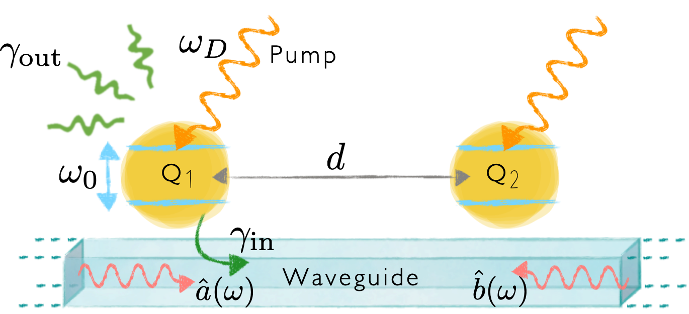
(a)

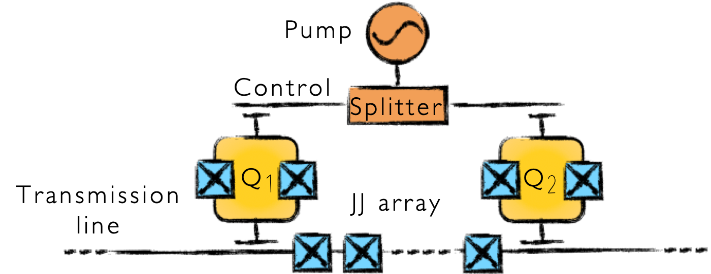
(b)

Figure 1: (a) Schematic representation of two emitters coupled to a one-dimensional waveguide, the qubits have a tunable resonance frequency of $\omega_{0}$ and are separated by a distance $d$ along the waveguide. Each qubit radiates into the waveguide with a rate $\gamma_{\mathrm{in}}$, and the dissipation rate outside the waveguide modes is $\gamma_{\mathrm{out}}$, with a total emission rate $\gamma\equiv\gamma_{\mathrm{in}}+\gamma_{\mathrm{out}}$. The qubits are pumped by an external driving field simultaneously. (b) Circuit QED implementation of the toy model with two transmon qubits Q1 and Q2 coupled to each other via a Josephson junction array, that is connected to transmission lines on each side Koch ; Yong19 ; Masluk12 . A split pump field drives the two qubits simultaneously via the control line. Further details of the setup are described in Section V and the parameter values pertaining to the model are summarized in Table 1, which we use throughout the paper to obtain results under realistic conditions. We assume the pump to be weak and symmetrically coupled to the two qubits with a Rabi frequency $\Omega$.

In a recent work superduper1 , the authors considered a simple model of two emitters coupled to a one-dimensional waveguide which captures the essential features of collective interactions under retardation. There, the focus was set on the spontaneous emission dynamics of certain emitter states, whereas the properties of the radiated field remained mostly unexplored. In this work, we extend the previous analyses of such a system in several ways: i) considering general initial states and atomic separations; ii) we show that the effective dipole-dipole interaction in the retarded regime decays exponentially with atomic separation; iii) we study the spectrum of the radiated field and unravel the features appearing due to non-Markovian effects; iv) Finally, we study the weakly driven situation to address the preparation of entangled states, considering an implementation of the model in circuit QED platforms, suggesting direct evidences of retarded collective effects that can be experimentally observed.

The paper is organized as follows. In Section II, we describe the model for the system in consideration as shown in Fig. 1(a). In Section III we study the undriven dynamics of the system in the single-excitation subspace. We analyse the response of the system under a weak external drive in Section IV, and present a possible superconducting circuit implementation of the model in Section V as depicted in Fig. 1(b). We summarize our results and outlook of this work in Section VI.

II Model

Let us consider a system of two distant two-level atoms coupled to a one-dimensional waveguide, as shown in Fig. 1 (a). One can understand why retardation renders such a system non-Markovian from a simple comparison of time scales. Considering the subsytems Q1 and Q2 to comprise the system system of interest and the EM field as the bath, the individual relaxation rate of each subsystem into the bath is $\gamma$, with a characteristic relaxation time scale $\tau_{\text{R}}\sim\gamma^{-1}$. The bath mediates the interactions between subsystems at a finite speed $v$, allowing us to define a time scale for bath correlations $\tau_{\text{B}}\sim d/v$. Once the system relaxation rate becomes comparable to the bath correlation time scale, or $\tau_{\text{R}}/\tau_{\text{B}}\sim\gamma d/v\equiv\eta\sim 1$, the Markov approximation is no longer valid BPbook . The parameter $\eta$ captures at least three different sources of non-Markovianity in the context of atom-light interactions Breuer16 ; deVega17 : (1) in the strong coupling regime as $\gamma$ increases Carlos13 ; Daniele19 , (2) for small propagation velocities Walther09 ; Mogilevtsev15 (such as close to a band gap or edge Thanopulos19 ; Vats98 ; John97 ; AGT2017PRA ; AGT2017PRL ; Krimer14 ), and (3) for large separations $d$, where the interaction between susbsystems is delayed superduper1 ; Whalen17 ; Grimsmo15 ; Tufarelli14 ; Guimond16 ; Dinc18 ; Dinc19 ; SPIE ; Carmele20 . Here we explore the system in a regime where the interatomic separation is such that $\eta\sim 1$, resulting in retardation-induced non-Markovian dynamics.

The Hamiltonian for a system of two atoms coupled to a waveguide and driven by an external pump field, as depicted in Fig. 1 (a) is $H=H_{\text{A}}+H_{\text{F}}+H_{\text{AF}}+H_{\text{AD}}$, where $H_{\text{A}}=\sum_{m=1,2}\hbar\omega_{0}\hat{\sigma}_{m}^{+}\hat{\sigma}_{m}^{-}$ is the Hamiltonian of the atoms, with $\hat{\sigma}_{m}^{\dagger}$ and $\hat{\sigma}_{m}$ as the raising and lowering operators for the $m^{\mathrm{th}}$ atom.

$$H_{\text{F}}=\int_{0}^{\infty}\mathrm{d}\omega\,\hbar\omega\left[\hat{a}^{\dagger}\left(\omega\right)\hat{a}\left(\omega\right)+\hat{b}^{\dagger}\left(\omega\right)\hat{b}\left(\omega\right)\right]$$ (1)

corresponds to the Hamiltonian for the guided modes of the electromagnetic field, with $\hat{a}\left(\omega\right)$ and $\hat{b}\left(\omega\right)$ referring to the right and left propagating modes. $H_{\text{AF}}$ and $H_{\text{AD}}$ describe the interaction of the atoms with the guided field and an external driving field, respectively.

Considering the interaction picture with respect to the free Hamiltonians $H_{0}=H_{\text{A}}+H_{\text{F}}$, the interaction Hamiltonians $\tilde{H}_{\text{AF}}\equiv e^{-iH_{0}t/\hbar}H_{\text{AF}}e^{iH_{0}t/\hbar}$ and $\tilde{H}_{\text{AD}}\equiv e^{-iH_{0}t/\hbar}H_{\text{AD}}e^{iH_{0}t/\hbar}$ can be written as follows.

$$\tilde{H}_{\text{AF}} =\sum_{m=1,2}\int_{0}^{\infty}\mathrm{d}\omega\,\hbar g\left(\omega\right)\left[\hat{\sigma}_{m}^{\dagger}\left\{\hat{a}\left(\omega\right)e^{ikx_{m}}+\hat{b}\left(\omega\right)e^{-ikx_{m}}\right\}e^{-i\left(\omega-\omega_{0}\right)t}+H.C.\right]$$ (2)

represents the interaction of the atoms with the waveguide modes within the electric-dipole and rotating wave approximations, wherein $g\left(\omega\right)$ corresponds to the coupling coefficient between the atoms and the field, and $x_{m}$ is the position of the $m^{\mathrm{th}}$ atom PierreBook .

$$\tilde{H}_{\text{AD}}= \hbar\Omega\sum_{m=1,2}\left[\hat{\sigma}_{m}^{\dagger}e^{-i\left(\omega_{\text{D}}-\omega_{0}\right)t}+\hat{\sigma}_{m}e^{i\left(\omega_{D}-\omega_{0}\right)t}\right]$$ (3)

is the semi-classical interaction of the emitters with a drive, where $\Omega$ is the Rabi frequency and $\omega_{\text{D}}$ is the drive frequency. One can use the driven Hamiltonian to prepare a particular collective atomic state. We explore this by first solving the problem without the drive for a single excitation subspace in Section III and use the solution to perturbatively calculate the weakly driven dynamics in Section IV Dorner02 .

III Dynamics without drive

Let us consider the system to be in the single-excitation subspace, where the dynamics is in the linear regime Calajo16 . The initial state contains one atomic excitation

$$\left|\Psi_{0}\right\rangle\equiv\left(\cos\theta\left|eg\right\rangle+\sin\theta e^{i\phi_{s}}\left|ge\right\rangle\right)\otimes\left|\left\{0\right\}\right\rangle,$$ (4)

with the waveguide field in the vacuum state $\left|\left\{0\right\}\right\rangle$. In the absence of a drive, the total Hamiltonian conserves the number of excitations such that we can use a Wigner-Weisskopf like ansatz to write the state of the atom+field system at a time $t$ as

$$\left|\Psi(t)\right\rangle= \left[\sum_{m=1,2}c_{m}(t)\hat{\sigma}_{m}^{+}+\int_{0}^{\infty}\mathrm{d}\omega\,\left\{c_{a}(\omega,t)\hat{a}^{\dagger}\left(\omega\right)(t)\right.\right.$$

$$\left.\left.+c_{b}(\omega,t)\hat{b}^{\dagger}\left(\omega\right)(t)\right\}\right]\left|gg\right\rangle\otimes\left|\left\{0\right\}\right\rangle,$$ (5)

where the coefficients $c_{m}(t)$ refer to the excitation amplitude for the $m^{\mathrm{th}}$ emitter and $c_{a(b)}(\omega,t)$ are the excitation amplitudes for the right (left)-propagating mode of the waveguide at frequency $\omega$.

The coupled equations of motion due to the atom-field interaction Hamiltonian $\tilde{H}_{\text{AF}}$ (Eq. (2)) are

$$\dot{c}_{a}\left(\omega,t\right)= -i\sum_{m=1,2}c_{m}\left(t\right)g\left(\omega\right)e^{-i\omega x_{m}/v}e^{i\left(\omega-\omega_{0}\right)t}$$ (6)

$$\dot{c}_{b}\left(\omega,t\right)= -i\sum_{m=1,2}c_{m}\left(t\right)g\left(\omega\right)e^{i\omega x_{m}/v}e^{i\left(\omega-\omega_{0}\right)t}$$ (7)

$$\dot{c}_{m}\left(t\right)= -i\int_{0}^{\infty}\mathrm{d}\omega\,g\left(\omega\right)e^{-i\left(\omega-\omega_{0}\right)t}$$

$$\left[c_{a}\left(\omega,t\right)e^{i\omega x_{m}/v}+c_{b}\left(\omega,t\right)e^{-i\omega x_{m}/v}\right].$$ (8)

Formally integrating (6) and (7), and substituting in (III) gives the equations of motion for the excitation amplitudes of the two atoms:

$$\dot{c}_{1}\left(t\right)= -\frac{\gamma}{2}\left[c_{1}\left(t\right)+\beta c_{2}\left(t-d/v\right)\Theta\left(t-d/v\right)e^{i\phi_{p}}\right],$$ (9)

$$\dot{c}_{2}\left(t\right)= -\frac{\gamma}{2}\left[c_{2}\left(t\right)+\beta c_{1}\left(t-d/v\right)\Theta\left(t-d/v\right)e^{i\phi_{p}}\right],$$ (10)

where we have defined $\phi_{p}\equiv d\omega_{0}/v$ as the phase accumulated by the field through its propagation between atoms. Assuming a sufficiently slowly varying density of modes around the atomic resonance, we define the emission into the waveguide as $\gamma_{\mathrm{in}}\equiv 4\pi\left|g\left(\omega_{0}\right)\right|^{2}$. $\gamma=\gamma_{\mathrm{in}}+\gamma_{\mathrm{out}}$ is the total spontaneous emission rate of the atom, which includes the radiation outside of the waveguide, which we add phenomenologically. The waveguide coupling efficiency $\beta=\gamma_{\mathrm{in}}/\gamma$ corresponds to the ratio of radiation emitted into the guided modes compared to the total emission. We neglect the effects of field propagation losses, a reasonable approximation for a waveguide based on a JJ array Masluk12 .

III.1 Atomic dynamics

The solutions of the system of coupled delay differential equations given by Eq. (9) and Eq. (10) have the form:

$$c_{1}\left(t\right)= K_{+}c_{+}\left(t\right)+K_{-}c_{-}\left(t\right),\text{ and}$$ (11)

$$c_{2}\left(t\right)= K_{+}c_{+}\left(t\right)-K_{-}c_{-}\left(t\right),$$ (12)

where $K_{\pm}\equiv\left\langle\Psi_{\pm}|\Psi_{0}\right\rangle=\left(\cos\theta\pm e^{i\phi_{s}}\sin\theta\right)/\sqrt{2}$ is the probability amplitude for the system being initially in the symmetric or anti-symmetric atomic states $\left|\Psi_{\pm}\right\rangle\equiv\frac{1}{\sqrt{2}}\left(\left|eg\right\rangle\pm\left|ge\right\rangle\right)\otimes\left|\left\{0\right\}\right\rangle$, and the functions $c_{\pm}\left(t\right)$ are the solutions to the delay differential equation

$$\frac{{d}c_{\pm}(t)}{{d}t}=-\frac{\gamma}{2}\left[c_{\pm}(t)\pm\beta e^{i\phi_{p}}c_{\pm}\left(t-\eta/\gamma\right)\Theta\left(t-\eta/\gamma\right)\right].$$ (13)

The effect of retardation enters in the second term on the right hand side and is characterized via two parameters, the delay time $\eta/\gamma$ $(=d/v)$ and the waveguide coupling efficiency times propagation phase factor $\beta e^{i\phi_{p}}$. The symmetry of the initial state combined with the phase accumulated by the field through propagation determine the overall phase difference of the interference. For example, the initial (anti-)symmetric state $\left|\Psi_{+}\right\rangle(\left|\Psi_{-}\right\rangle)$ with propagation phase $\phi_{p}=2p\pi~{}(\phi_{p}=(2p+1)\pi)$ is superradiant, while $\left|\Psi_{-}\right\rangle(\left|\Psi_{+}\right\rangle)$ with a propagation phase $\phi_{p}=2p\pi~{}(\phi_{p}=(2p+1)\pi)$ is subradiant (where $p\in\mathbb{Z}$).

III.1.1 Solution in terms of Lambert-$W$ functions

Equation (13) can be solved in terms of Lambert-$W$ functions as superduper1 ; Asl03

$$c_{\pm}(t)=\frac{1}{\sqrt{2}}\sum_{n=-\infty}^{\infty}\alpha_{n}^{(\pm)}e^{-\gamma_{n}^{(\pm)}t/2}$$ (14)

with

$$\gamma_{n}^{(\pm)} ={\gamma}\left[1-\frac{W_{n}\left(\mp\frac{\eta}{2}e^{\eta/2}\beta e^{i\phi_{p}}\right)}{\eta/2}\right]$$ (15)

$$\alpha_{n}^{(\pm)} =\left[1+W_{n}\left(\mp\frac{\eta}{2}e^{\eta/2}\beta e^{i\phi_{p}}\right)\right]^{-1},$$ (16)

where $W_{n}(x)$ is the $n^{\mathrm{th}}$ branch of the Lambert $W$-function, that often occurs in solutions to delayed-feedback problems Corless96 . The coefficients $\alpha_{n}^{\left(\pm\right)}$ and $\gamma_{n}^{(\pm)}$ are generally complex valued.

We notice that the largest contribution to the sum comes from the terms $n=\left\{-1,0,1\right\}$, capturing the qualitative dynamics of the system (see supplemental material in superduper1 , for example). Particularly, for the symmetric state, $\gamma_{0}^{(+)}$ is real valued for $\eta<\eta_{c}$, where $\eta_{c}\equiv 2W_{0}(\frac{1}{\beta e})$ is defined as a critical distance between the emitters below which there are no oscillations in the atomic dynamics superduper1 . Nonetheless, higher order terms are necessary to guarantee the convergence to the correct solution. These terms $(n\neq 0)$ also contribute to the effective spontaneous emission rate, which has been previously calculated only from the $n=0$ term superduper1 ; Dinc19 ; Zheng13 , an issue that requires careful treatment (see Apeendix B for more details).

III.1.2 Solution in terms of wavepacket multiple reflections

We can write an alternative solution to the dynamics as follows Milonni74

$$c_{\pm}\left(t\right)=\frac{1}{\sqrt{2}}\sum_{n=0}^{\infty} \left[\frac{\left(\mp\beta e^{i\phi_{p}}\right)^{n}}{n!}\left(\frac{\gamma t-n\eta}{2}\right)^{n}\right.$$

$$\left.e^{-\left(\gamma t-n\eta\right)/2}\Theta\left(t-\frac{n\eta}{\gamma}\right)\right].$$ (17)

The above expansion can be understood in terms of a cascade of processes as the field emitted by each of the atoms propagates back and forth between them at signaling times of $t=nd/v$. The field then coherently adds to the existing amplitudes, offering the intuition that the decay dynamics arises from the multiple partial reflections of a field wavepacket bouncing between the atoms.

Although the two solutions in Eq. (14) and Eq. (III.1.2) appear different, they are equivalent, providing complementary insights in the dynamics of systems with self-consistent time-delayed feedback superduper1 .

III.1.3 Effective decay rates in presence of retardation

From the full solution of the dynamics for the two atoms, we can define an effective instantaneous atomic decay rate for the $m^{\mathrm{th}}$ atom as

$$\gamma^{\mathrm{eff}}_{m}\equiv-2\mathrm{Re}\left[\frac{1}{c_{m}(t)}\frac{{d}c_{m}(t)}{{d}t}\right].$$ (18)

Substituting Eq. (11) and Eq. (13) in Eq. (18), we find that

$$\gamma_{1,2}^{\mathrm{eff}}\left(t\right)=\gamma\left(1+\mathrm{Re}\left[\beta e^{i\phi_{p}}\frac{c_{2,1}\left(t-\eta/\gamma\right)}{c_{1,2}(t)}\right]\right),$$ (19)

The first term corresponds to the individual atomic decay rate, while the second term corresponds to the modification due to a second atom with a delayed interaction, such that its amplitude is evaluated at a retarded time $t\rightarrow t-\eta/\gamma$, corresponding to the delay time between the two atoms. This illustrates that collective spontaneous emission can be understood as a mutually stimulated emission of two dipoles Cray82 .

Let us consider the atoms to be initially in a symmetric or anti-symmetric state, with an amplitude $c_{\pm}\left(t\right)$ corresponding to the states $\left|\Psi_{\pm}\right\rangle$ ($K_{+}=0$ or $K_{-}$=0 respectively). After the field emitted by one atom reaches the other, namely $d/v<t<2d/v$, the excitation amplitudes for the symmetric and anti-symmetric states can be written from Eq. (11) and Eq. (III.1.2) as

$$c_{\pm}\left(t\right)=\frac{1}{\sqrt{2}}\left[e^{-\gamma t/2}\mp\beta e^{i\phi_{p}}\left(\frac{\gamma t-\eta}{2}\right)e^{-\left(\gamma t-\eta\right)/2}\right],$$ (20)

The corresponding instantaneous rate of spontaneous emission for $t\rightarrow\frac{d}{v}^{+}$ is

$$\lim_{t\rightarrow\frac{d}{v}^{+}}\gamma^{\mathrm{eff}}_{\pm}=\gamma\left(1\pm\beta\cos\phi_{p}e^{\eta/2}\right).$$ (21)

Further assuming that $\beta\cos\phi_{p}=1$, we note that the instantaneous emission rate for a pair of initially symmetric dipoles $\gamma_{+}^{\mathrm{eff}}$ can exceed $2\gamma$, a feature referred to as superduperradiance superduper1 . We also observe from Eq. (21) that $\gamma_{-}^{\mathrm{eff}}$ could be negative, illustrating that an initially asymmetric state can exhibit recoherence, exciting the atoms after they have decayed .

III.1.4 Energy shifts from retarded dipole-dipole interaction

The energy shift due to the retarded resonant dipole-dipole interaction can be defined as Milonni15

$$\Delta^{\mathrm{eff}}_{m}(t)\equiv-2\mathrm{Im}{\left[c^{\ast}_{\mathrm{m}}(t)\frac{{d}c_{\mathrm{m}}(t)}{{d}t}\right]}.$$ (22)

For a general initial state the shift at any time $t$ is given as,

$$\Delta_{1,2}^{\mathrm{eff}}\left(t\right)=\gamma\beta\mathrm{Im}\left[e^{i\phi_{p}}c_{1,2}^{\ast}\left(t\right)c_{2,1}\left(t-\eta/\gamma\right)\right].$$ (23)

Considering the two atoms to be initially in a symmetric or anti-symmetric state, the instantaneous shift at ${\frac{d}{v}}<t<{\frac{2d}{v}}$ can be found from substituting Eq. (20) in Eq. (22) as

$$\lim_{t\rightarrow{\frac{d}{v}}^{+}}\Delta_{\pm}^{\mathrm{eff}}(t)=\pm\frac{\gamma}{2}e^{-\eta/2}\beta\sin\phi_{p}.$$ (24)

Comparing the above with the effective instantaneous emission rate $\gamma^{\mathrm{eff}}_{\pm}$ in Eq. (21) we note that the two are related to each other as the real and imaginary part of a common response function PeterQOBook .

We further remark that for small distances the dipole-dipole interaction is oscillatory $(\sim\sin\phi_{p})$ Milonni15 , as predicted by a Markov approximation. Upon including retardation, the dipole-dipole interaction decays exponentially with distance, with the coherence length of the spontaneously emitted photon $(\sim v/\gamma)$ determining the characteristic length scale. This suggests that dipole-dipole interactions in one-dimension cannot be truly infinite-ranged Solano2017 because of retardation, setting another limit to the range of collective emitter interactions in one-dimensional systems beyond the ones discussed in Ref. SanchezBurillo20 .

III.2 Field dynamics and spectrum

Having written the atomic dynamics, we now consider the dynamics of the electromagnetic field modes and the spectrum of the field, which is defined as the probability of finding a photon of frequency $\omega$ in the waveguide modes at any given time. We substitute the solution for atomic dynamics in Eq. (11) into the equations of motion for the field in Eq. (6) and Eq. (7) to obtain the field excitation amplitude as follows

$$c_{a}\left(\omega,t\right)=-i\sqrt{\frac{\beta\gamma}{\pi}} \left[K_{+}\cos\left(\frac{kd}{2}\right)F_{+}(\omega,t)\right.$$

$$\left.-iK_{-}\sin\left(\frac{kd}{2}\right)F_{-}(\omega,t)\right]$$ (25)

$$c_{b}\left(\omega,t\right)=-i\sqrt{\frac{\beta\gamma}{\pi}} \left[K_{+}\cos\left(\frac{kd}{2}\right)F_{+}(\omega,t)\right.$$

$$\left.+iK_{-}\sin\left(\frac{kd}{2}\right)F_{-}(\omega,t)\right]$$ (26)

where we have defined

$$F_{\pm}\left(\omega,t\right)= \int_{0}^{t}\mathrm{d}\tau\,c_{\pm}\left(\tau\right)e^{i\left(\omega-\omega_{0}\right)\tau}.$$ (27)

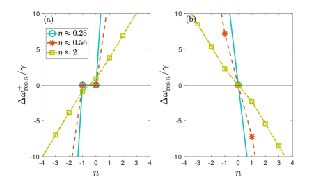
Figure 2: Shift in the resonant frequency $\Delta\omega^{\pm}_{\mathrm{res},n}$ corresponding to the different branches of the $W$-function for the initial (a) symmetric and (b) anti-symmetric states. The prominent contributions to the total spectrum are due to $n=\left\{-1,0\right\}$ for the symmetric case, and $n=\left\{-1,0,1\right\}$ for the antisymmetric case superduper1 . It can be seen from (a) that for small enough atomic separations $(\eta<\eta_{c})$ there is no shift to the prominent resonance peaks $(\Delta\omega^{+}_{\mathrm{res},n}\approx 0)$ corresponding to $n=\left\{-1,0\right\}$. The $\eta$ values are chosen such that $\phi_{p}=\eta\omega_{0}/\gamma=2p\pi$.

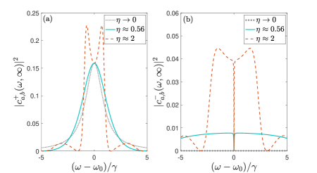
(a)

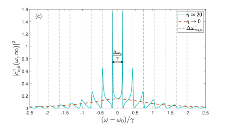
(b)

Figure 3: Steady state excitation probability of waveguide modes as a function of frequency for different interatomic separations for initial (a) symmetric and (b) antisymmetric states. It can be deduced numerically from (a) that the FWHM of the late-time spectrum for $\eta\approx 0.56$ is $\Delta_{\mathrm{FWHM}}\approx 2.57$ which exceeds that for the case of coincident emitters $\eta=0$ ($\Delta_{\mathrm{FWHM}}\approx 1.97$, which in the limit of perfect coupling to the waveguide with $\beta\rightarrow 1$ approaches $\Delta_{\mathrm{FWHM}}\rightarrow 2$), this is a signature for retardation-induced modification to collective atomic decay. For $\eta>\eta_{c}$, there are multiple peaks in the late time spectrum for the initial symmetric state. (c) Late time spectrum for $\eta\approx 20$ for an initial symmetric state is depicted as the solid blue curve. The self phase modulation dynamics in the atomic cavity leads to Fano resonance-like spectrum. The spacing between each resonant peak is roughly given as $\Delta\omega_{c}/\gamma\approx 0.286$ from Eq. (31). The dashed vertical lines represent the resonance frequency peaks $\Delta\omega_{\mathrm{res},n}^{+}$ given in Eq. (29). The width of the central resonant peak is given by Eq. (30) as $\gamma_{\mathrm{res},0}^{+}\approx 0.0083\gamma$. The red dashed curve corresponds to the superradiant spectrum for two coincident emitters $(\eta\rightarrow 0)$. The $\eta$ values are chosen such that $\phi_{p}=\eta\omega_{0}/\gamma=2p\pi$.

In the late time limit, $t\rightarrow\infty$, we obtain

$$F^{\infty}_{\pm}(\omega)=\frac{i}{\sqrt{2}}\sum_{n\in\mathbb{Z}}\frac{\alpha_{n}^{(\pm)}}{\left[\left(\omega-\omega_{0}\right)-\Delta\omega_{\mathrm{res},n}^{\pm}\right]+i\gamma_{\mathrm{res},n}^{\pm}/2},$$ (28)

which illustrates that there are multiple resonant peaks in the outgoing field spectrum at frequencies $\left(\omega_{0}+\Delta\omega_{\mathrm{res},n}^{\pm}\right)$ with a corresponding width $\gamma_{\mathrm{res},n}^{\pm}$. The resonance frequency shifts $\Delta\omega_{\mathrm{res},n}^{\pm}$ and widths $\gamma_{\mathrm{res},n}$ are given by

$$\Delta\omega_{\mathrm{res},n}^{\pm} =-\frac{\gamma}{\eta}\mathrm{Im}\left[W_{n}\left(\mp\beta e^{i\phi_{p}}\frac{\eta}{2}e^{\eta/2}\right)\right]$$ (29)

$$\gamma_{\mathrm{res},n}^{\pm} =\gamma\left[1-\frac{2}{\eta}\mathrm{Re}\left[W_{n}\left(\mp\beta e^{i\phi_{p}}\frac{\eta}{2}e^{\eta/2}\right)\right]\right].$$ (30)

Note that the steady state field spectrum is the Fourier transform of the transient atomic dynamics, thus the lineshifts and linewidths obtained above are in agreement with Eq. (14). Fig. 2 shows the resonance frequencies for different $n$ values. We note from Fig. 2 (a) that for small enough atomic separations $\eta<\eta_{c}$, there is no shift in the resonance peaks for the symmetric spectrum for $n=0,-1$, the dominant orders.

Figure 3 shows the spectrum of field radiated outside the system. For a value of $\eta<\eta_{c}$, the spectrum has a single maximum. This can be understood from the fact that for small enough atomic separation the late time spectrum has only one resonance at $\omega\approx\omega_{0}$ as seen in Fig. 3 (a). In this limit the two atoms behave as a single entity. For distances $\eta>\eta_{c}$, we see that there are two prominent peaks corresponding to $\Delta\omega_{\mathrm{res,n}}^{+}$ with $n=-1,0$. This corresponds to the limit where the two atoms make an effective cavity and interact with the field oscillating within. In the case of a symmetric atomic state (see Fig. 3 (a)), the spectral width of the spectrum as defined via its full width at half-maximum (FWHM) increases as a signature of the enhancement of the spontaneous emission beyond Dicke superradiance.

In the case of an anti-symmetric atomic state (see Fig. 3 (b)), the spectrum is ideally zero, since a perfect subradiant states does not radiate light for $\eta=0$. However, for $\eta>0$, a broad spectrum appears from the field that leaks out of the system before the atoms interact with each other, suddenly turning it off once the atoms “see” each other and destructively interfere. This turn-off process contributes with a broad range of frequency components. In the case of anti-symmetric emitters, there is always a narrow dip at $\omega=\omega_{0}$. This is because the resonant radiation into the waveguide is mostly trapped in the region between the emitters, but over time it can be scattered out into external modes. The dip in the center is therefore determined by the waveguide coupling efficiency $\beta$.

In the long cavity limit, meaning $\eta>1$, the field wavepacket radiated by the atoms is reflected multiple times within the effective cavity formed by the atoms. The resulting output field is a train of pulses separated by a time $d/v$. In the frequency domain this results in multiple resonance peaks as seen in Fig. 3(c). Each resonant peak corresponds to a Lorentzian in Eq. (28), that are all phase coherent with each other. The asymmetry of each peak arises from a Fano-like interference between the atomic resonance and the resonances of the cavity made by the atoms Fano .

For the case of a symmetric initial state, the separation between the central resonant peak is given by

$$\Delta\omega_{c}=\frac{2\gamma}{\eta}\mathrm{Im}\left[W_{0}\left(-\beta\frac{\eta}{2}e^{\eta/2}\right)\right].$$ (31)

As the two atoms are separated infinitely further apart, $\lim_{\eta\rightarrow\infty}\mathrm{Im}\left[W_{0}\left(-\beta\frac{\eta}{2}e^{\eta/2}\right)\right]=\pi$. Thus the spacing between different teeth asymptotically approaches ${\Delta\omega_{c}}/\left(2\pi\right)\rightarrow v/d$. This is twice the free spectral range of a Fabry-Perot cavity of length $d$, with ${\Delta\omega_{\mathrm{FSR}}}/\left(2\pi\right)=v/(2d)$ PierreBook . This can be understood from the fact that while for a cavity the field leaks out after every round trip time $(2d/v)$, in the two atom system, the field leaks out of the atomic “cavity” after every half-round trip $d/v$. The correspondence to a cavity only applies as an asymptotic behaviour when the atoms are placed far apart, but in a general scenario the free spectral range in Eq. (31) is determined by the delayed feedback effects between the two atoms.

The late time spectrum can be alternatively written in a more physically intuitive form by substituting the series solution for the atomic dynamics given in Eq. (III.1.2) into Eq. (27) as (see Appendix A for proof)

$$F_{\pm}^{\infty}(\omega)=\frac{i}{\sqrt{2}}\frac{1}{\left[\left(\omega-\omega_{0}\right)\mp\frac{\gamma\beta}{2}\sin\left(\frac{\omega\eta}{\gamma}\right)\right]+i\frac{\gamma}{2}\left[1\pm\beta\cos\left(\frac{\omega\eta}{\gamma}\right)\right]}.$$ (32)

In the limit of coincident atoms, $\eta\rightarrow 0$, $F_{\pm}^{\infty}\left(\omega\right)\sim\frac{1}{\left(\omega-\omega_{0}\right)+i\frac{\gamma}{2}\left(1\pm\beta\right)}$, we recover a Lorentzian spectrum for the field PierreBook . This gives us the expected Dicke super- and sub-radiant emission profiles for $\beta\rightarrow 1$ with a spectrum peak at $\omega=\omega_{0}$ and linewidths $\gamma^{\pm}=2\gamma,0$. Deviations from the Lorentzian profile are yet another signature that the dynamics is non-Markovian due to the retardation effects. It can be seen that the usual Lorentzian spectrum of the atoms in the Markovian limit is modified by a frequency dependent phase modulation factor $\sim\frac{\gamma\beta}{2}e^{i\phi_{p}}$ $(\phi_{p}=\omega\eta/\gamma)$, the real part of which $\left(\frac{\gamma\beta}{2}\cos\left(\omega\eta/\gamma\right)\right)$ contributes to the linewidth modification and the imaginary part $\left(\frac{\gamma\beta}{2}\sin\left(\omega\eta/\gamma\right)\right)$ to the resonant lineshift. This can be understood as coming from the propagation phase $\phi_{p}$ for the field modes as they traverse the interatomic distance and interfere with their time-delayed amplitudes. One can also derive the resonant peaks $\left(\omega_{0}+\Delta\omega^{\pm}_{\mathrm{res},n}\right)$ and corresponding linewidths $\gamma^{\pm}_{\mathrm{res},n}$ (as in Eq. (29) and Eq. (30)) from Eq. (32) as shown in Appendix B. The above spectrum is also similar to that emitted from a single excited atom placed in front of a mirror in a retarded regime Dorner02 . The two problems correspond to each other via image theory.

IV Driven dynamics

We now add a weak drive to the atomic system as given by the interaction Hamiltonian $\tilde{H}_{\text{AD}}$ in Eq. (3) to address the collective state preparation. Notice that the drive Hamiltonian does not conserve the total number of excitations in the atom+field system. Since solving the equations of motion for multiple excitations in the presence of non-Markovian feedback is analytically hard, we solve the driven dynamics perturbatively within the linear regime Dorner02 , assuming that the Rabi frequency is sufficiently small $(\Omega\lesssim\gamma)$.

Let us assume that the atoms are initially in the ground state and the field in the waveguide is in vacuum, as

$$\left|\Psi_{0}\right\rangle\equiv\left|gg\right\rangle\otimes\left|\left\{0\right\}\right\rangle.$$ (33)

Considering that the interaction with the drive is switched on at $t=0$ we can write the amplitudes of excitation for the symmetric and anti-symmetric states $\left|\Psi_{\pm}\right\rangle$ as $c_{\pm}^{D}\left(t\right)$ at a time $t$ from first order perturbation theory, obtaining

$$c_{\pm}^{D}\left(t\right) =-\frac{i}{\hbar}\int_{0}^{t}\mathrm{d}\tau\left\langle\Psi_{\pm}\right|e^{i\tilde{H}_{\text{AF}}\tau/\hbar}\tilde{H}_{\text{AD}}e^{-i\tilde{H}_{\text{AF}}\tau/\hbar}\left|\Psi_{0}\right\rangle$$

$$=-i\sqrt{2}\Omega\int_{0}^{t}\mathrm{d}\tau\,e^{i\left(\omega_{0}-\omega_{D}\right)\tau}\left\langle\Psi_{\pm}\right|e^{i\tilde{H}_{\text{AF}}\tau/\hbar}\left|\Psi_{+}\right\rangle.$$ (34)

This implies that the drive perturbatively excites the atoms into a single excitation symmetric state $\left|\Psi_{+}\right\rangle$ by the virtue of a weak symmetric coupling (see Eq. (3)), which then evolves in the linear regime via the atom-field interaction Hamiltonian $\tilde{H}_{\text{AF}}$. We note however that while the atomic state is symmetric, for a propagation phase $\phi_{p}=(2p+1)\pi$, the two atoms behave subradiantly ChangNJP ; Mirhosseini19 . In the presence of retardation effects such subradiant states can evolve into highly delocalized entangled states such as the BIC states superduper1 ; SPIE ; Calajo19 .

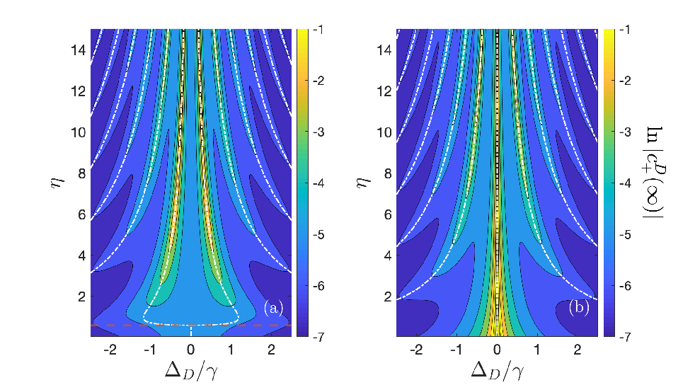
Figure 4: Late time excitation probability for the symmetric state as a function of the drive detuning and atomic separation. The $\eta$ values are chosen such that for (a) $\phi_{p}=\eta\omega_{0}/\gamma=2p\pi$, which corresponds to the superradiant state and (b) $\phi_{p}=\eta\omega_{0}/\gamma=(2p+1)\pi$ corresponding to the subradiant state. The steady state atomic excitation probability as a function of the drive detuning has multiple peaks at $\omega_{D}=\omega_{0}-\Delta\omega_{\mathrm{res},n}^{+}$ as determined by Eq. (29), as depicted by the dashed-dotted white curves. As the atomic separation increases the number of peaks increases similar to the Fano resonance-like structure of the late time spectrum in Fig. 3 (c). The red dashed line in (a) represnts the critical distance $\eta=\eta_{c}$ after which there is a bifurcation of the central peak. It can be seen that in a subradiant configuration Rabi frequency for the weak driving field is $\Omega=0.1\gamma$.

The steady state excitation amplitude for the symmetric state can be thus obtained from Eq.(34)

$$c_{+}^{D}\left(t\rightarrow\infty\right)=\Omega\sum_{n}\,\frac{{\alpha_{n}^{(+)}}^{\ast}}{(\omega_{D}-\omega_{0}+\Delta\omega^{+}_{\mathrm{res},n})+i\gamma^{+}_{\mathrm{res},n}},$$ (35)

where $\Delta\omega_{\mathrm{res},n}^{+}$ and $\gamma_{\mathrm{res},n}^{+}$ are as defined in Eq. (29) and Eq. (30) respectively. Thus we note that there are multiple peaks in the steady state atomic amplitude for a drive frequency such that $\omega_{D}=\omega_{0}-\Delta\omega_{\mathrm{res},n}^{+}$, with a corresponding width of $\gamma_{\mathrm{res},n}^{+}$. Similar to Eq. (32), this can be alternatively written as

$$c_{+}^{D}\left(t\rightarrow\infty\right)$$

$$=\frac{\Omega}{\left[\Delta_{D}+\beta\frac{\gamma}{2}\sin\left(\frac{\omega_{D}\eta}{\gamma}\right)\right]+i\frac{\gamma}{2}\left[1+\beta\cos\left(\frac{\omega_{D}\eta}{\gamma}\right)\right]},$$ (36)

where $\Delta_{D}=\omega_{0}-\omega_{D}$ is the drive detuning. In the limit of the two emitters being coincident, we find that the excitation amplitude $c_{+}^{D}\left(t\rightarrow\infty\right)\rightarrow\frac{\Omega}{\Delta_{D}+i\frac{\gamma}{2}\left(1+\beta\right)}$ is described by the familiar Lorentzian profile as a function of the detuning $\Delta_{D}$ with a width $\gamma\left(1+\beta\right)/2$ PierreBook .

Figure  4 shows the symmetric state excitation probability in the late time limit as a function of the drive detuning and atomic separation, for the specific propagation phases of $\phi_{p}=2p\pi,(2p+1)\pi$ which correspond to a superradiant and a subradiant pair of emitters respectively. We observe multiple peaks in the excitation probability corresponding to drive frequencies $\omega_{D}=\omega_{0}-\Delta\omega_{\mathrm{res},n}^{+}$ as determined by Eq. (35).

This scheme can be used to prepare two distant atoms in an entangled state, depending upon the drive detuning and the atomic separation. We remark however that these results are limited by the applicability of perturbation theory and require the drive strength to be sufficiently weak. The dynamics of the scattered field is discussed in Appendix D. While for weak driving one only sees the elastic scattering process, in the general case of a strong drive, this would correspond to the resonance fluorescence spectrum of two emitters with retarded interaction Lenz93 .

V Superconducting circuit implementation

The model and results described here can be implemented in a circuit QED (cQED) setup. Specifically, we consider a setup with two transmon qubits with resonance frequency $\omega_{0}\approx 5$ GHz coupled to a Josephson junction (JJ) array as shown in Fig. 1(b). We further assume that the two qubits are driven simultaneously by an external pump that couples symmetrically to both. We describe the details of the JJ array in Appendix C, and summarize the parameters value in Table 1. For such values, as detailed in Appendix C, a distance of $d\approx 1.6$ cm between the qubits corresponds to an $\eta\approx 1$, where the system would exhibit significant retardation effects. These parameters are within the fabrication capabilities of ongoing experiments Leger19 ; Kuzmin19 .

Collective effects in cQED have been already observed in a system of two artificial atoms coupled to a microwave cavity vanloo13 ; Mlynek14 , and recent implementations have extended their study to multi-qubit systems Mirhosseini19 ; Wang20 . Moreover, waveguides made of JJ arrays with low dissipation losses can significantly decrease the field velocity Masluk12 ; Kuzmin19 . It is within the reach of current experiments to put both elements together and demonstrate collective atom-field dynamics with retardation effects.

Qubit resonance frequency $\omega_{0}/(2\pi)$	5 GHz
Decay rate $\gamma/(2\pi)$	10 MHz
Waveguide coupling efficiency $\beta$	0.95
Phase velocity $v/c$	1/300

Table 1: Parameter values for a superconducting circuit implementation of the model as depicted in Fig. 1 (b). We use this parameters throughout the paper to present our results under realistic conditions.

VI Summary and Discussion

To summarize, we study a system of two driven distant emitters coupled to a one-dimensional waveguide considering retardation effects. We analytically solve the dynamics of the system for a general initial atomic state in the single-excitation subspace. We illustrate the collective atomic decay as mutually-induced stimulated emission process (see Eq. (21)). We also show that dipole-dipole interactions decay exponentially as a function of the interatomic distance, with a characteristic length scale determined by the linewidth of the field (see Eq. (24)). We find that the spectrum of the radiated field can exhibit a linewidth broadening beyond that of standard Dicke superradiance (Fig. 3(a)). Additionally, if the atoms are widely separated, the spectrum of the field exhibits Fano resonance-like peaks, shown in Fig. 3(b). We finally consider a weak drive in the system, to prepare entangled atomic steady states, and determine the parameters of the drive that allow the preparation of a particular collective state. We further illustrate that one can realize the model in a cQED implementation, with parameter values within reach of the state-of-the-art setups.

As an outlook, this work represents a step forward towards the study of strongly driven dynamics in the retarded regime. While we have explored the dynamics in a single-excitation regime, its extension to multiple excitations in the system, can exhibit non-linear and distinctly quantum features. As an example of such regime, one can consider the modifications to the resonance fluorescence spectrum of two atoms due to retardation Lenz93 . Given the present analysis of two emitters coupled to a waveguide, the study of multiple emitters seems a natural extension, as recently explored in Ref. Dinc19 by studying the atomic dynamics. It would be interesting to explore the linewidth and coherence properties of the narrow frequency peaks in the radiation spectrum in the many-atom scenario Khan18 . Additionally, circuit QED setups with tunable qubit frequencies and engineerable JJ arrays allow for implementing a determined spectral density of modes that can help with efficient steady state entanglement generation between the qubits Hartmann08 ; Zueco12 .

VII Acknowledgement

We are specially grateful to Pierre Meystre for inspiring discussions throughout the course of the work. We also thank Peter W. Milonni, Luis A. Orozco, Elizabeth A. Goldschmidt, Hakan E. Türeci, and Saeed A. Khan for insightful comments and thoughtful reading of the manuscript. K.S acknowledges helpful discussions with Ahreum Lee, Hyok Sang Han, Fredrik K. Fatemi and S. L. Rolston. A. G.-T. acknowledges support from the Spanish project PGC2018-094792-B-100 (MCIU/AEI/FEDER, EU) and from the CSIC Research Platform on Quantum Technologies PTI-001. Y.L. acknowledges the Knut, Alice Wallenberg Foundation, and the Swedish Research Council for financial support. P.S. was supported by CONICYT-PAI grants 77190033. K.S. acknowledges support from the US Department of Energy, Office of Basic Energy Sciences, Division of Materials Sciences and Engineering, under Award No. DE-SC0016011.

Appendix A Late time field dynamics

Substituting the series solution for the atomic dynamics Eq. (III.1.2) in Eq. (27)

$$F_{\pm}\left(t\rightarrow\infty\right)= \lim_{t\rightarrow\infty}\frac{1}{\sqrt{2}}\int_{0}^{t}\mathrm{d}\tau e^{i\left(\omega-\omega_{0}\right)\tau}\sum_{n=0}^{\infty}\frac{\left(\mp\beta e^{i\phi_{p}}\right)^{n}}{n!}\left(\frac{\gamma\tau-n\eta}{2}\right)^{n}e^{-\left(\gamma\tau-n\eta\right)/2}\Theta\left(\gamma\tau-n\eta\right).$$ (37)

Let us define $\tilde{\tau}\equiv\frac{\gamma\tau-n\eta}{2}$, to rewrite the above as

$$F_{\pm}\left(t\rightarrow\infty\right)=\frac{1}{\sqrt{2}}\sum_{n=0}^{\infty}\frac{\left(\mp\beta e^{i\phi_{p}}\right)^{n}}{n!}\left(\frac{2}{\gamma}e^{i\left(\omega-\omega_{0}\right)n\eta/\gamma}\right)\left[\int_{0}^{\infty}\mathrm{d}\tilde{\tau}\tilde{\tau}^{n}e^{-\tilde{\tau}}\Theta\left(\tilde{\tau}\right)e^{2i\left(\omega-\omega_{0}\right)\tilde{\tau}/\gamma}\right].$$ (38)

Now using the Laplace transform identity $\int_{0}^{\infty}\mathrm{d}xe^{-sx}x^{n}e^{-\alpha x}\Theta\left(x\right)=\frac{n!}{(s+\alpha)^{n+1}},$ we can simplify the integral in the square bracket above to obtain

$$F_{\pm}\left(t\rightarrow\infty\right)=$$

$$\frac{1}{\sqrt{2}\left[\frac{\gamma}{2}-i\left(\omega-\omega_{0}\right)\right]}\sum_{n=0}^{\infty}\left[\mp\frac{\beta e^{i{\omega\eta/\gamma}}}{\left\{1-2i\left(\omega-\omega_{0}\right)/\gamma\right\}}\right]^{n}$$ (39)

which yields Eq. (32) using the identity $\sum_{n=0}^{\infty}x^{n}=\frac{1}{1-x}$, for $\left|x\right|<1$, which is ensured from the coupling efficiency $\beta$ being less than 1.

Appendix B Resonant peaks in late time spectrum

Let us consider the characteristic equation for resonant peaks from the denominator in Eq. (32)

$$\bar{\omega}^{\pm}-\omega_{0}+i\frac{\gamma}{2}\pm i\frac{\gamma\beta}{2}e^{i\bar{\omega}\eta/\gamma}=0.$$ (40)

Defining $\tilde{\omega}^{\pm}=\left(\bar{\omega}^{\pm}-\omega_{0}+i\frac{\gamma}{2}\right)$,

$$\tilde{\omega}^{\pm}\pm i\frac{\gamma\beta}{2}e^{i\eta/\gamma\left[\tilde{\omega}+\omega_{0}-i\gamma/2\right]}=0$$ (41)

$$\implies \left(-i\frac{\tilde{\omega}\eta}{\gamma}\right)e^{-i\tilde{\omega}\eta/\gamma}=\mp\beta e^{i\phi_{p}}\frac{\eta}{2}e^{\eta/2}$$ (42)

$$\implies -i\frac{\tilde{\omega}_{n}\eta}{\gamma}=W_{n}\left(\mp\beta e^{i\phi_{p}}\frac{\eta}{2}e^{\eta/2}\right),$$ (43)

where we have used the definition of the Lambert-$W$ function that $W(x)=f^{-1}(x)$, with $f(x)=xe^{x}$. This yields the complex eigenvalue of the characteristic equation as

$$\bar{\omega}_{n}^{\pm}= \omega_{0}-i\frac{\gamma}{2}+i\frac{\gamma}{\eta}W_{n}\left(\mp\beta e^{i\phi_{p}}\frac{\eta}{2}e^{\eta/2}\right)$$ (44)

$$= \omega_{0}-i\frac{\gamma_{n}^{(\pm)}}{2},$$ (45)

where we have used Eq. (15). The real and imaginary part of the above yields the resonant peak frequencies $\omega_{0}+\Delta\omega_{\mathrm{res},n}^{\pm}$ and the corresponding linewidths $\gamma_{\mathrm{res},n}^{\pm}$ of the late time spectrum as in Eq. (29) and (30).

We further remark that Eq. (40) is the characteristic equation used in solving the atomic dynamics in Refs. Dinc19 ; Zheng13 , though in these works only the zeroth eigenvalue is considered. This gives an effective decay rate that corresponds to only $\gamma^{\pm}_{\mathrm{res},n=0}$. However the full solution to the dynamics includes other eigenvalues as well, and yields an effective decay rate that differs from superduper1 ; Dinc19 ; Zheng13 .

Appendix C Josephson junction array as waveguide

We consider two transmon qubits with a resonance frequency $\omega_{0}$ coupled to a JJ array made of $N\approx 2000$ identical JJs in series, as shown in Fig. 1 (b). The schematic for a JJ array is depicted in Fig. 5. Assuming that the JJs are linear such that each JJ can be treated as an LC oscillator, one can derive the dispersion relation for such a waveguide, following the approach in Masluk12 such that

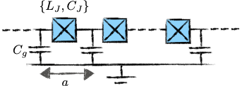
Figure 5: Schematic representation of a JJ array circuit. Each JJ, represented in blue is considered to be a linear $LC$-oscillator with an inductance $L_{J}\approx 1$ nH and capacitance $C_{J}\approx 1$ fF, and is connected to the ground with a capacitance $C_{g}\approx 100$ fF. Each unit cell is of length $a\approx 10$ $\mu$m.

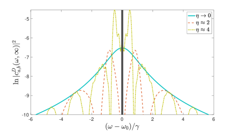
Figure 6: Scattering spectrum from a pair of driven emitters at different separations. The propagation phase is assumed to be $\phi_{p}=2p\pi$. The solid line at $\omega=\omega_{0}$ denotes that the resonant frequency is being filtered.

$$\omega(k)=\frac{1}{\sqrt{L_{J}C_{J}}}\sqrt{\frac{1-\cos\left(ka\right)}{\frac{C_{g}}{2C_{J}}+\left(1-\cos\left(ka\right)\right)}},$$ (46)

where $ka=n\pi/N$. With the chosen parameter values for $L_{J}$, $C_{J}$ and $C_{g}$ as indicated in Fig. 5, the phase velocity of the field around $\omega_{0}\approx 5$ GHz is $v=\omega/k\approx 1\times 10^{6}$ m/s.

Appendix D Driven field spectrum with retardation

The driven symmetric state amplitude can be obtained from Eq. (34) as

$$c_{+}^{D}\left(t\right)= -\Omega\sum_{n\in\mathbb{Z}}{\alpha_{n}^{(+)}}^{\ast}\frac{e^{\left[i\Delta_{D}-{\gamma_{n}^{(+)}}^{\ast}/2\right]t}-1}{\Delta_{D}+i{\gamma_{n}^{(+)}}^{\ast}/2},$$ (47)

where $\Delta_{D}\equiv\omega_{0}-\omega_{D}$ is the detuning of the laser with respect to the atomic resonance. We note that the above expression for the atomic excitation amplitude is similar to that for the field amplitude in Eq. (27) with $\omega\rightarrow\omega_{D}$, and thus exhibits the similar features as those in Section III.2.

We consider the dynamics of the waveguide modes as sourced by the two atoms. The excitation amplitudes of the field modes are obtained by substituting Eq. (47) in Eq. (6) and Eq. (7), and subsequently integrating those to yield

$$c_{a,b}^{D}\left(\omega,t\right)= -\Omega\sqrt{\frac{\beta\gamma}{\pi}}\cos\left(\frac{kd}{2}\right)\sum_{n}\frac{{\alpha_{n}^{(+)}}^{\ast}}{i\Delta_{D}-{\gamma_{n}^{(+)}}^{\ast}/2}$$

$$\left[\frac{e^{\left\{i\left(\omega-\omega_{D}\right)-{\gamma_{n}^{(+)}}^{\ast}/2\right\}t}-1}{i\left(\omega-\omega_{D}\right)-{\gamma_{n}^{(+)}}^{\ast}/2}-\frac{e^{{i\left(\omega-\omega_{0}\right)}t}-1}{i\left(\omega-\omega_{0}\right)}\right]$$ (48)

The first term in the above expression is due to the field emitted from symmetric state transient dynamics, while the second term corresponds to the field emitted in the steady state. Given the weak driving assumption, this corresponds to only the elastic scattering process in the resonance fluorescence spectrum Lenz93 .

We consider the two terms in the above separately in the steady state. It can be shown that in the late time limit, the second term corresponds to an infinitely sharp resonant peak, as $\lim_{t\rightarrow\infty}\frac{e^{i\left(\omega-\omega_{0}\right)t}-1}{\omega-\omega_{0}}\sim\delta\left(\omega-\omega_{0}\right)$. Assuming that the resonant peak can be filtered, the first term in the steady state limit becomes

$$c_{a,b}^{D}\left(\omega,t\right) =-\Omega\sqrt{\frac{\beta\gamma}{\pi}}\cos\left(\frac{kd}{2}\right)$$

$$\sum_{n}\left[\frac{1}{\Delta_{D}+i{\gamma_{n}^{(+)}}^{\ast}/2}\right]\frac{{\alpha_{n}^{(+)}}^{\ast}}{{\left(\omega-\omega_{D}\right)+i{\gamma_{n}^{(+)}}^{\ast}/2}}.$$ (49)

Thus we note from the above that the scattered field has resonant peaks at $\omega=\omega_{D}+\Delta\omega_{\mathrm{res},n}^{+}$, with corresponding widths $\gamma_{\mathrm{res},n}^{+}$. The scattered field spectrum is plotted in Fig. 6. The multiple peaks for a pair of distant emitters are a signature of retardation effects.

References

- (1) R. H. Dicke, Coherence in Spontaneous Radiation Processes, Phys. Rev. 93, 99 (1954).
- (2) M. Gross, and S. Haroche, Superradiance: An essay on the theory of collective spontaneous emission, Phys. Rep. 93, 301 (1982).
- (3) D. S. Dovzhenko, S. V. Ryabchuk, Yu. P. Rakovich, and I. R. Nabiev, Light-matter interaction in the strong coupling regime: configurations, conditions, and applications, Nanoscale, 10, 3589 (2018).
- (4) Y. Todorov, A. M. Andrews, R. Colombelli, S. De Liberato, C. Ciuti, P. Klang, G. Strasser, and C. Sirtori, Ultrastrong Light-Matter Coupling Regime with Polariton Dots, Phys. Rev. Lett. 105, 196402 (2010).
- (5) Q. Zhang, M. Lou, X. Li, J. L. Reno, W. Pan, J. D. Watson, M. J. Manfra, and J. Kono, Collective non-perturbative coupling of 2D electrons with high-quality-factor terahertz cavity photons, Nature Phys. 12, 1005 (2016).
- (6) J. Flick, N. Rivera, and P. Narang, Strong light-matter coupling in quantum chemistry and quantum photonics, Nanophotonics, 7, 1479, (2018).
- (7) K. Hammerer, A. S. Sørensen, and E. S. Polzik, Quantum interface between light and atomic ensembles, Rev. Mod. Phys. 82, 1041 (2010).
- (8) M. D. Lukin, M. Fleischhauer, R. Cote, L. M. Duan, D. Jaksch, J. I. Cirac, and P. Zoller, Dipole Blockade and Quantum Information Processing in Mesoscopic Atomic Ensembles, Phys. Rev. Lett. 87, 037901 (2001).
- (9) M. Saffman, T. G. Walker, and K. Mølmer, Quantum information with Rydberg atoms, Rev. Mod. Phys. 82, 2313 (2010).
- (10) A. E. B. Nielsen and K. Mølmer, Deterministic multimode photonic device for quantum-information processing, Phys. Rev. A 81, 043822 (2010).
- (11) P. Zanardi and M. Rasetti, Noiseless Quantum Codes, Phys. Rev. Lett. 79, 3306 (1997).
- (12) D. A. Lidar, and K. B. Whaley, Decoherence-Free Subspaces and Subsystems, Springer Lect. Notes Phys. 622, 83 (2003).
- (13) G. Facchinetti, S. D. Jenkins, and J. Ruostekoski, Storing Light with Subradiant Correlations in Arrays of Atoms, Phys. Rev. Lett. 117, 243601 (2016).
- (14) A. Asenjo-Garcia, M. Moreno-Cardoner, A. Albrecht, H. J. Kimble, D. E. Chang, Exponential improvement in photon storage fidelities using subradiance and "selective radiance" in atomic arrays, Phys. Rev. X 7, 031024 (2017).
- (15) J. A Needham, I. Lesanovsky, and B. Olmos, Subradiance-protected excitation transport, New J. Phys. 21, 073061 (2019).
- (16) J. Galego, F. Garcia-Vidal, and J. Feist, Suppressing photochemical reactions with quantized light fields, Nat. Commun. 7, 13841 (2016).
- (17) M. Hertzog, M. Wang, J. Mony, and K. Börjesson, Strong light-matter interactions: a new direction within chemistry, Chem. Soc. Rev., 48, 937 (2019).
- (18) A. N. Poddubny, Collective Förster energy transfer modified by a planar metallic mirror, Phys. Rev. B 92, 155418 (2015).
- (19) X. Zhong, T. Chervy, L. Zhang, A. Thomas, J. George, C. Genet, J. A. Hutchison, and T. W. Ebbesen, Energy Transfer between Spatially Separated Entangled Molecules, Angew. Chem. Int. Ed. 56, 9034 (2017).
- (20) M. Gómez-Castaño, A. Redondo-Cubero, L. Buisson, J. L. Pau, A. Mihi, S. Ravaine, R. A. L. Vallée, A. Nitzan, M. Sukharev, Energy Transfer and Interference by Collective Electromagnetic Coupling, Nano Lett. 19, 5790 (2019).
- (21) R. Röhlsberger, K. Schlage1, B. Sahoo, S. Couet, and R. Rüffer, Collective Lamb Shift in Single-Photon Superradiance, Science, 328, 1248 (2010).
- (22) P. Y. Wen, K.-T. Lin, A. F. Kockum, B. Suri, H. Ian, J. C. Chen, S. Y. Mao, C. C. Chiu, P. Delsing, F. Nori, G.-D. Lin, and I.-C. Hoi, Large Collective Lamb Shift of Two Distant Superconducting Artificial Atoms, Phys. Rev. Lett. 123, 233602 (2019).
- (23) K. Sinha, B. P. Venkatesh, and P. Meystre, Collective Effects in Casimir-Polder Forces, Phys. Rev. Lett. 121, 183605 (2018).
- (24) S. Fuchs, and S. Y. Buhmann, Purcell-Dicke enhancement of the Casimir-Polder potential, Eur. Phys. Lett. 124, 34003 (2018).
- (25) W. Guerin, M. T. Rouabah, and R. Kaiser, Light interacting with atomic ensembles: collective, cooperative and mesoscopic effects, J. Mod. Opt. 64, 895 (2017).
- (26) N. Skribanowitz, I. P. Herman, J. C. MacGillivray, and M. S. Feld, Observation of Dicke Superradiance in Optically Pumped HF Gas, Phys. Rev. Lett. 30, 309 (1973).
- (27) M. Gross, C. Fabre, P. Pillet, S. Haroche, Observation of Near-Infrared Dicke Superradiance on Cascading Transitions in Atomic Sodium, Phys. Rev. Lett. 36, 1035 (1976).
- (28) D. Pavolini, A. Crubellier, P. Pillet, L. Cabaret, and S. Liberman, Experimental Evidence for Subradiance, Phys. Rev. Lett. 54, 1917 (1985).
- (29) R. G. DeVoe and R. G. Brewer, Observation of Superradiant and Subradiant Spontaneous Emission of Two Trapped Ions, Phys. Rev. Lett. 76, 2049 (1996).
- (30) P. Solano, P. Barberis-Blostein, F. K. Fatemi, L. A. Orozco, S. L. Rolston, Super-radiance reveals infinite-range dipole interactions through a nanofiber, Nat. Commun. 8, 1857 (2017).
- (31) P. Solano, J. A. Grover, J. E. Hoffman, S. Ravets, F. K. Fatemi, L. A. Orozco, S. L. Rolston, Optical Nanofibers: A New Platform for Quantum Optics, Adv. At. Mol. Opt. Phys. 66, 439 (2017).
- (32) P. Solano, Quantum Optics in Optical Nanofibers, Doctoral Thesis (2017).
- (33) C. A. Ebongue, D. Holzmann, S. Ostermann, and H. Ritsch, Generating a stationary infinite range tractor force via a multimode optical fibre, J. Opt. 19, 065401 (2017).
- (34) S. Kato, N. Német, K. Senga, S. Mizukami, X. Huang, S. Parkins, and T. Aoki, Observation of dressed states of distant atoms with delocalized photons in coupled-cavities quantum electrodynamics, Nat. Commum. 10, 1160 (2019).
- (35) R. J. Schoelkopf and S. M. Girvin, Wiring up quantum systems, Nature 451, 664 (2008).
- (36) A. González-Tudela, V. Paulisch, D. E. Chang, H. J. Kimble, and J. I. Cirac, Deterministic Generation of Arbitrary Photonic States Assisted by Dissipation, Phys. Rev. Lett. 115, 163603 (2015).
- (37) J. Ruostekoski, and J. Javanainen, Emergence of correlated optics in one-dimensional waveguides for classical and quantum atomic gases, Phys. Rev. Lett. 117, 143602 (2016).
- (38) E. Shahmoon, and G. Kurizki, Nonradiative interaction and entanglement between distant atoms, Phys. Rev. A 87, 033831 (2013).
- (39) A. González-Tudela, V. Paulisch, H. J. Kimble, and J. I. Cirac, Efficient Multiphoton Generation in Waveguide Quantum Electrodynamics, Phys. Rev. Lett. 118, 213601 (2017).
- (40) W. Ge, K. Jacobs, Z. Eldredge, A. V. Gorshkov, and M. Foss-Feig, Distributed Quantum Metrology with Linear Networks and Separable Inputs Phys. Rev. Lett. 121, 043604 (2018).
- (41) H.-P. Breuer, and F. Petruccione, Theory of open quantum systems (Oxford University Press, New York, 2002).
- (42) K. Sinha, P. Meystre, E. Goldschmidt, F. K. Fatemi, S. L. Rolson, P. Solano, Non-Markovian collective emission from macroscopically separated emitters, Phys. Rev. Lett. 124, 043603 (2020).
- (43) P. W. Milonni and P. L. Knight, Retardation in the resonant interaction of two identical atoms, Phys. Rev. A 10, 1096 (1974).
- (44) P. W. Milonni, and P. L. Knight, Retardation in coupled dipole-oscillator systems, Am. J. Phys. 44, 741 (1976).
- (45) P. R. Berman, Theory of two atoms in a chiral waveguide, Phys. Rev. A 101, 013830 (2020).
- (46) H. P. Breuer, E. M. Laine, J. Piilo, and B. Vacchini, Colloquium: Non-Markovian dynamics in open quantum systems, Rev. Mod. Phys. 88, 021002 (2016).
- (47) I. de Vega, and D. Alonso, Dynamics of non-Markovian open quantum systems, Rev. Mod. Phys. 89, 015001 (2017).
- (48) H. Gießen, J. D. Berger, G. Mohs, P. Meystre, and S. F. Yelin, Cavity-modified spontaneous emission: From Rabi oscillations to exponential decay, Phys. Rev. A 53, 2816 (1996).
- (49) U. Dorner and P. Zoller, Laser-driven atoms in half-cavities, Phys. Rev. A 66, 023816 (2002).
- (50) T. Tufarelli, F. Ciccarello, and M. S. Kim, Dynamics of spontaneous emission in a single-end photonic waveguide, Phys. Rev. A 87, 013820 (2013).
- (51) T. Tufarelli, M. S. Kim, and F. Ciccarello, Non-Markovianity of a quantum emitter in front of a mirror, Phys. Rev. A 90, 012113 (2014).
- (52) A. Carmele, J. Kabuss, F. Schulze, S. Reitzenstein, and A. Knorr, Single Photon Delayed Feedback: A Way to Stabilize Intrinsic Quantum Cavity Electrodynamics, Phys. Rev. Lett. 110, 013601 (2013).
- (53) R. J. Cook and P. W. Milonni, Quantum theory of an atom near partially reflecting walls, Phys. Rev. A 35, 5081 (1987).
- (54) P.-O. Guimond, A. Roulet, H. N. Le, and V. Scarani, Rabi oscillation in a quantum cavity: Markovian and non-Markovian dynamics, Phys. Rev. A 93, 023808 (2016).
- (55) F. Dinç, A. M. Brańczyk, I. Ercan, Real-space time dynamics in waveguide QED: bound states and single-photon-pulse scattering, Quantum 3, 213 (2019).
- (56) F. Dinc and A. M. Braǹczyk, Non-Markovian super-superradiance in a linear chain of up to 100 qubits, Phys. Rev. Research 1, 032042(R) (2019).
- (57) K. Sinha, P. Meystre, P. Solano, Non-Markovian dynamics of collective atomic states coupled to a waveguide, Quantum Nanophotonic Materials, Devices, and Systems 11091 (2019).
- (58) C. W. Hsu, B. Zhen, A. D. Stone, J. D. Joannopoulos, and M. Soljačić, Bound states in the continuum, Nat. Rev. Mat. 1, 16048 (2016).
- (59) P. T. Fong and C. K. Law, Bound state in the continuum by spatially separated ensembles of atoms in a coupled-cavity array, Phys. Rev. A 96, 023842 (2017).
- (60) G. Calajó, Y.-L. L. Fang, H. U. Baranger, and F. Ciccarello, Exciting a Bound State in the Continuum through Multiphoton Scattering Plus Delayed Quantum Feedback, Phys. Rev. Lett. 122, 073601 (2019).
- (61) P. Facchi, D. Lonigro, S. Pascazio, F. V. Pepe, D. Pomarico, Bound states in the continuum for an array of quantum emitters, Phys. Rev. A 100, 023834 (2019).
- (62) P. Facchi, M. S. Kim, S. Pascazio, F. V. Pepe, D. Pomarico, and T. Tufarelli,Bound states and entanglement generation in waveguide quantum electrodynamics, Phys. Rev. A 94, 043839 (2016).
- (63) L. Guo, A. F. Kockum, F. Marquardt, and G. Johansson, Oscillating bound states for a giant atom, arXiv:1911.13028 (2019).
- (64) H. Zheng and H. U. Baranger, Persistent Quantum Beats and Long-Distance Entanglement from Waveguide-Mediated Interactions, Phys. Rev. Lett. 110, 113601 (2013).
- (65) H. Pichler and P. Zoller, Photonic Circuits with Time Delays and Quantum Feedback, Phys. Rev. Lett. 116, 093601 (2016).
- (66) J. Koch, T. M. Yu, J. Gambetta, A. A. Houck, D. I. Schuster, J. Majer, Alexandre Blais, M. H. Devoret, S. M. Girvin, and R. J. Schoelkopf, Charge-insensitive qubit design derived from the Cooper pair box, Phys. Rev. A 76, 042319 (2007).
- (67) Y. Lu, A. Bengtsson, J. J. Burnett, E. Wiegand, B. Suri, P. Krantz, A. F. Roudsari, A. F. Kockum, S. Gasparinetti, G. Johansson, P. Delsing , Characterizing decoherence rates of a superconducting qubit by direct microwave scattering, arXiv:1912.02124 (2019).
- (68) N. A. Masluk, I. M. Pop, A. Kamal, Z. K. Minev, and M. H. Devoret, Microwave Characterization of Josephson Junction Arrays: Implementing a Low Loss Superinductance, Phys. Rev. Lett. 109, 137002 (2012).
- (69) S. Longhi, Opt. Lett. 45, 3297 (2020).
- (70) C. Gonzalez-Ballestero, F. J. García-Vidal, and E. Moreno, Non-Markovian effects in waveguide-mediated entanglement, New J. Phys. 15, 073015 (2013).
- (71) D. De Bernardis, T. Jaako, and P. Rabl, Cavity quantum electrodynamics in the nonperturbative regime, Phys. Rev. A 97, 043820 (2018).
- (72) D. Mogilevtsev, E. Reyes-Gómez, S. B. Cavalcanti, and L. E. Oliveira, Slow light in semiconductor quantum dots: Effects of non-Markovianity and correlation of dephasing reservoirs, Phys. Rev. B 92, 235446 (2015).
- (73) A. Walther, A. Amari, S. Kröll, and A. Kalachev, Experimental superradiance and slow-light effects for quantum memories, Phys. Rev. A 80, 012317 (2009).
- (74) I. Thanopulos, V. Karanikolas, N. Iliopoulos, E. Paspalakis, Non-Markovian spontaneous emission dynamics of a quantum emitter near a MoS2 nanodisk, arXiv:1904.09264 (2019).
- (75) N. Vats and S. John, Non-Markovian quantum fluctuations and superradiance near a photonic band edge, Phys. Rev. A 58, 4168 (1998).
- (76) S. John and T. Quang, Collective Switching and Inversion without Fluctuation of Two-Level Atoms in Confined Photonic Systems, Phys. Rev. Lett. 78, 1888 (1997).
- (77) A. González-Tudela and J. I. Cirac, Markovian and non-Markovian dynamics of quantum emitters coupled to two-dimensional structured reservoirs, Phys. Rev. A 96, 043811 (2017).
- (78) A. González-Tudela and J. I. Cirac, Quantum Emitters in Two-Dimensional Structured Reservoirs in the Nonperturbative Regime, Phys. Rev. Lett. 119, 143602 (2017).
- (79) D. O. Krimer, M. Liertzer, S. Rotter, and H. E. Türeci, Route from spontaneous decay to complex multimode dynamics in cavity QED, Phys. Rev. A 89, 033820 (2014).
- (80) S. J. Whalen, A. L. Grimsmo, and H. J. Carmichael, Open quantum systems with delayed coherent feedback, Quantum Sci. Technol. 2, 044008 (2017).
- (81) A. L. Grimsmo, Time-Delayed Quantum Feedback Control, Phys. Rev. Lett. 115, 060402 (2015).
- (82) A. Carmele, N. Nemet, V. Canela, and S. Parkins, Pronounced non-Markovian features in multiply excited, multiple emitter waveguide QED: Retardation-induced anomalous population trapping, Phys. Rev. Research 2, 013238 (2020).
- (83) R. Kuzmin, N. Mehta, N. Grabon, R. Mencia, and V. E. Manucharyan, Superstrong coupling in circuit quantum electrodynamic, npj Quantum Inf. 5, 20 (2019).
- (84) P. Meystre and M. Sargent, Elements of Quantum Optics (Springer-Verlag, Berlin, 2007).
- (85) G. Calajo, F. Ciccarello, D. E. Chang, and P. Rabl, Atom-field dressed states in slow-light waveguide QED, Phys. Rev. A 93, 033833 (2016).
- (86) F. M. Asl, and A. G. Ulsoy, Analysis of a System of Linear Delay Differential Equations, J. Dyn. Sys., Meas., Control 125, 215 (2003).
- (87) R. M. Corless, G. H. Gonnet, D. E. G. Hare, D. J. Jeffrey, D. E. Knuth, On the Lambert- function, Adv. Comput. Math. 5, 329 (1996).
- (88) M. Cray, M.-L. Shih, and P. W. Milonni, Stimulated emission, absorption, and interference, Am. J. Phys. 50, 1016 (1982).
- (89) P. W. Milonni, S. M. H. Rafsanjani, Distance dependence of two-atom dipole interactions with one atom in an excited state, Phys. Rev. A 92, 062711 (2015).
- (90) P. W. Milonni, An introduction to quantum optics and quantum fluctuations, Oxford University Press, 2019.
- (91) E. Sánchez-Burillo, D. Porras, A. González-Tudela, On the limits of photon-mediated interactions in one-dimensional photonic baths, arXiv:2003.07854 (2020).
- (92) U. Fano, Effects of Configuration Interaction on Intensities and Phase Shifts, Phys. Rev. 124, 1866 (1961).
- (93) D. E. Chang, L. Jiang, A. V. Gorshkov, and H. J. Kimble, Cavity QED with atomic mirrors, New J. Phys. 14 063003, (2012).
- (94) G. Lenz and P. Meystre, Resonance fluorescence from two identical atoms in a standing-wave field, Phys. Rev. A 48, 3365 (1993).
- (95) S. Léger, J. Puertas-Martínez, K. Bharadwaj, R. Dassonneville, J. Delaforce, F. Foroughi, V. Milchakov, L. Planat, O. Buisson, C. Naud, W. Hasch-Guichard, S. Florens, I. Snyman, and N. Roch, Observation of quantum many-body effects due to zero point fluctuations in superconducting circuits, Nat. Commun. 10, 5259 (2019).
- (96) S. Khan, and H. E. Türeci, Frequency Combs in a Lumped-Element Josephson-Junction Circuit, Phys. Rev. Lett. 120, 153601 (2018).
- (97) A. F. van Loo, A. Fedorov, K. Lalumiére, B. C. Sanders, A. Blais, and A. Wallraff, Photon-Mediated Interactions Between Distant Artificial Atoms, Science 342, 1494 (2013).
- (98) J. A. Mlynek, A. A. Abdumalikov, C. Eichler, and A. Wallraff, Observation of Dicke superradiance for two artificial atoms in a cavity with high decay rate, Nat. Commun. 5, 5186 (2014).
- (99) M. Mirhosseini, E. Kim, X. Zhang, A. Sipahigil, P. B. Dieterle, A. J. Keller, A. Asenjo-Garcia, D. E. Chang, and O. Painter, Cavity quantum electrodynamics with atom-like mirrors, Nature 569, 692 (2019).
- (100) Z. Wang, H. Li, W. Feng, X. Song, C. Song, W. Liu, Q. Guo, X. Zhang, H. Dong, D. Zheng, H. Wang, and D.-W. Wang, Controllable Switching between Superradiant and Subradiant States in a 10-qubit Superconducting Circuit, Phys. Rev. Lett. 124, 013601 (2020).
- (101) M. Hartmann, F. G. S. L. Brandão, and M. Plenio, Quantum many-body phenomena in coupled cavity arrays, Laser Photonics Rev. 2, 527 (2008).
- (102) D. Zueco, J. J. Mazo, E. Solano, and J. J. García-Ripoll, Microwave photonics with Josephson junction arrays: Negative refraction index and entanglement through disorder, Phys. Rev. B 86, (2012).