CO emission in distant galaxies on and above the main sequence

We present the detection of multiple carbon monoxide CO line transitions with ALMA in a few tens of infrared-selected galaxies on and above the main sequence at $z=1.1-1.7$. We reliably detected the emission of CO $(5-4)$, CO $(2-1)$, and CO $(7-6)$+[C I]$(^{3}P_{2}\,-\,^{3}P_{1})$ in 50, 33, and 13 galaxies, respectively, and we complemented this information with available CO $(4-3)$ and [C I]$(^{3}P_{1}\,-\,^{3}P_{0})$ fluxes for part of the sample, and modeling of the optical-to-mm spectral energy distribution. We retrieve a quasi-linear relation between $L_{\rm IR}$ and CO $(5-4)$ or CO $(7-6)$ for main-sequence galaxies and starbursts, corroborating the hypothesis that these transitions can be used as star formation rate (SFR) tracers. We find the CO excitation to steadily increase as a function of the star formation efficiency (SFE), the mean intensity of the radiation field warming the dust ($\langle U\rangle$), the surface density of SFR ($\Sigma_{\rm SFR}$), and, less distinctly, with the distance from the main sequence ($\Delta\mathrm{MS}$). This adds to the tentative evidence for higher excitation of the CO+[C I] spectral line energy distribution (SLED) of starburst galaxies relative to that for main-sequence objects, where the dust opacities play a minor role in shaping the high-$J$ CO transitions in our sample. However, the distinction between the average SLED of upper main-sequence and starburst galaxies is blurred, driven by a wide variety of intrinsic shapes. Large velocity gradient radiative transfer modeling demonstrates the existence of a highly excited component that elevates the CO SLED of high-redshift main-sequence and starbursting galaxies above the typical values observed in the disk of the Milky Way. This excited component is dense and it encloses $\sim 50$% of the total molecular gas mass in main-sequence objects. We interpret the observed trends involving the CO excitation as mainly driven by a combination of large SFRs and compact sizes, as large $\Sigma_{\rm SFR}$ are naturally connected with enhanced dense molecular gas fractions and higher dust and gas temperatures, due to increasing UV radiation fields, cosmic ray rates, and dust/gas coupling. We release the full data compilation and the ancillary information to the community.

1 Introduction

Since its first detection in external galaxies a few decades ago, the prominent role of the molecular gas in determining the evolution of galaxies has been established by constantly growing evidence, and interpreted by progressively more sophisticated theoretical arguments (e.g., Young & Scoville, 1991; Solomon & Vanden Bout, 2005; Carilli & Walter, 2013; Hodge & da Cunha, 2020, for reviews).

On the one hand, the detection of tens of different molecular transitions in local molecular clouds and resolved nearby galaxies, spanning a wide range of properties, allowed for a detailed description of the processes regulating the physics of the interstellar medium (ISM). On the other hand, the observation of a handful of species and lines in unresolved galaxies at various redshifts has been instrumental to identify the main transformations that galaxy populations undergo with time. In particular, it is now clear that the majority of galaxies follows a series of scaling relations connecting their star formation rates (SFRs), the available molecular and atomic gas reservoirs ($M_{\rm gas}$, $M_{\rm HI}$) and their densities and temperatures, the stellar and dust masses ($M_{\star}$, $M_{\rm dust}$), metallicities ($Z$), sizes, and several other properties derived from the combination of these parameters. Two relations received special attention in the past decade: the so-called “main sequence” (MS) of star-forming galaxies, a quasi-linear and relatively tight ($\sigma\sim 0.3$ dex) correlation between $M_{\star}$ and SFR (Brinchmann et al., 2004; Noeske et al., 2007; Daddi et al., 2007; Elbaz et al., 2007; Rodighiero et al., 2011; Whitaker et al., 2012; Speagle et al., 2014; Sargent et al., 2014; Schreiber et al., 2015); and the Schmidt-Kennicutt (SK) relation between the surface densities of SFR and gas mass ($\Sigma_{\rm SFR}-\Sigma_{\rm gas}$, Schmidt, 1959; Kennicutt, 1998). Only a minor fraction of massive star-forming galaxies, dubbed “starbursts” (SBs), deviate from the MS, displaying exceptional SFRs for their $M_{\star}$ (Rodighiero et al., 2011), and potentially larger $\Sigma_{\rm SFR}$ at fixed $\Sigma_{\rm gas}$ (Daddi et al., 2010a; Sargent et al., 2014; Casey et al., 2014). These objects are generally related to recent merger events, at least in the local Universe, and they can be easily spotted as bright beacons in the far-infrared and (sub)millimeter regimes, owing to their strong dust emission exceeding $L_{\rm IR}>10^{11-12}$ $L_{\odot}$ ((Ultra)-Luminous InfraRed Galaxies, (U)LIRGs, Sanders & Mirabel, 1996).

It has also become evident that the normalization of the MS rapidly increases with redshift: distant galaxies form stars at higher paces than in the local Universe, at fixed stellar mass (e.g., Daddi et al., 2007; Elbaz et al., 2007; Whitaker et al., 2012; Speagle et al., 2014; Schreiber et al., 2015). This trend could be explained by the availability of copious molecular gas at high redshift (Daddi et al., 2010a; Tacconi et al., 2010; Scoville et al., 2017a; Tacconi et al., 2018; Riechers et al., 2019; Decarli et al., 2019; Liu et al., 2019b), ultimately regulated by the larger accretion rates from the cosmic web (Kereš et al., 2005; Dekel et al., 2009a). Moreover, higher SFRs could be induced by an increased efficiency of star formation due to the enhanced fragmentation in gas-rich, turbulent, and gravitationally unstable high-redshift disks (Bournaud et al., 2007; Dekel et al., 2009b; Bournaud et al., 2010; Ceverino et al., 2010; Dekel & Burkert, 2014), reflected on their clumpy morphologies (Elmegreen et al., 2007; Förster Schreiber et al., 2011; Genzel et al., 2011; Guo et al., 2012, 2015; Zanella et al., 2019). IR-bright galaxies with prodigious SFRs well above the level of the MS are observed also in the distant Universe, but their main physical driver is a matter of debate. While a star formation efficiency ($\mathrm{SFE}=\mathrm{SFR}/M_{\rm gas}$) monotonically increasing with the distance from the main sequence ($\Delta\mathrm{MS}=\mathrm{SFR/SFR_{MS}}$, Genzel et al. 2010; Magdis et al. 2012; Genzel et al. 2015; Tacconi et al. 2018, 2020) could naturally explain the existence of these outliers, recent works suggest the concomitant increase of gas masses as the main driver of the starbursting events (Scoville et al., 2016; Elbaz et al., 2018). In addition, if many bright starbursting (sub)millimeter galaxies (SMGs, Smail et al., 1997) are indeed merging systems as in the local Universe (Gómez-Guijarro et al., 2018, and references therein), there are several well documented cases of SMGs hosting orderly rotating disks at high redshift (e.g., Hodge et al., 2016, 2019; Drew et al., 2020), disputing the pure merger scenario. The same definition of “starbursts” as galaxies deviating from the main sequence has been recently questioned with the advent of high spatial resolution measurements of their dust and gas emission. Compact galaxies with short depletion timescales typical of SBs are now routinely found on the MS, being possibly on their way to leave the sequence (Barro et al., 2017a; Popping et al., 2017; Elbaz et al., 2018; Gómez-Guijarro et al., 2019; Puglisi et al., 2019; Jiménez-Andrade et al., 2019); or galaxies moving within the MS scatter, due to mergers unable to efficiently boost the star formation (Fensch et al., 2017) or owing to gravitational instabilities and gas radial redistribution (Tacchella et al., 2016).

In this framework, a primary source of confusion stems from the relatively limited amount of information available for sizable samples of high-redshift galaxies, homogeneously selected on and above the main sequence. While a fine sampling of the far-IR spectral energy distribution (SED) has now become more accessible and a fundamental source to derive properties as the dust mass, temperature, and luminosity (e.g., Simpson et al., 2014; Scoville et al., 2016; Dunlop et al., 2017; Brisbin et al., 2017; Strandet et al., 2017; Franco et al., 2018; Zavala et al., 2018; Liu et al., 2019a; Dudzevičiūtė et al., 2019; Simpson et al., 2020; Hodge & da Cunha, 2020, to mention a few recent high-resolution surveys in the (sub)mm), direct spectroscopic measurements of the cold gas in distant galaxies remain remarkably time consuming. As a result, systematic investigations of the gas properties focused on either one line transition in large samples of galaxies (e.g., Le Fèvre et al., 2019; Freundlich et al., 2019; Tacconi et al., 2018, 2020), or several lines in sparser samples, often biased towards the brightest objects as (lensed) SMGs or quasars (e.g., Carilli & Walter, 2013; Bothwell et al., 2013; Spilker et al., 2014; Yang et al., 2017; Cañameras et al., 2018; Dannerbauer et al., 2019). Moreover, the spectroscopic study of normal MS galaxies at high redshift has been primarily devoted to the determination of the total molecular gas masses and fractions via the follow-up of low-$J$ carbon monoxide transitions (CO $(1-0)$ to CO $(3-2)$, Dannerbauer et al. 2009; Daddi et al. 2010a; Tacconi et al. 2010; Freundlich et al. 2019; Tacconi et al. 2020), with a few exceptions ([C I], Valentino et al. 2018, 2020; Bourne et al. 2019; Brisbin et al. 2019; [C II], Capak et al. 2015; Zanella et al. 2018; Le Fèvre et al. 2019). Little is known about the denser and warmer phases in distant normal disks, but these components might hold the key to reach a deeper understanding of the galaxy growth, being naturally associated with the star-forming gas.

A few pilot studies specifically targeting mid-$J$ CO transitions in MS galaxies suggest the existence of significant pockets of such dense/warm molecular gas up to $z\sim 3$ (Daddi et al., 2015; Brisbin et al., 2019; Cassata et al., 2020), along with more routinely detected large cold reservoirs traced by low-$J$ lines (Dannerbauer et al., 2009; Aravena et al., 2010, 2014). The observed CO line luminosities of moderately excited transitions as CO $(5-4)$ further correlate almost linearly with the total IR luminosity $L_{\rm IR}$ (Daddi et al., 2015), similarly to what is observed for local IR bright objects and distant SMGs (Greve et al., 2014; Liu et al., 2015a; Lu et al., 2015, 2017; Kamenetzky et al., 2016), suggesting their potential use as SFR tracers. Moreover, these studies show evidence of CO spectral line energy distributions (SLEDs) significantly more excited in MS galaxies than what observed in the Milky Way, but less than local (U)LIRGs and high-redshift SMGs (Dannerbauer et al., 2009; Daddi et al., 2015; Cassata et al., 2020). While not necessarily good proxies of the mode of star formation (secular vs bursty) per se, (CO) SLEDs are relevant if they can constrain the fraction of dense molecular gas (Daddi et al., 2015), and they remain a precious source of information on the processes heating and exciting the ISM. This has been extensively proven by detailed studies of local galaxies, including spirals, ongoing mergers, starbursts, and active nuclear regions (Panuzzo et al., 2010; Papadopoulos et al., 2010b, a; Rangwala et al., 2011; Papadopoulos et al., 2012; Kamenetzky et al., 2012; Schirm et al., 2014; Lu et al., 2014; Wu et al., 2015; Mashian et al., 2015; Rosenberg et al., 2015; Kamenetzky et al., 2016, 2017; Lu et al., 2017; Lee et al., 2019, among the others). However, the study of warm and dense molecular gas in distant MS galaxies remains limited to a handful of objects to date.

Here we present the first results of a new multi-cycle campaign with the Atacama Large Millimeter Array (ALMA), whose impressive capabilities allowed for the survey of several species in the span of a few minutes of on-source integration. We targeted multiple CO (CO $(2-1)$, CO $(4-3)$, CO $(5-4)$, CO $(7-6)$) and neutral atomic carbon ([C I]$(^{3}P_{1}\,-\,^{3}P_{0})$, [C I]$(^{3}P_{2}\,-\,^{3}P_{1})$) line emissions in a sample of a few tens of main-sequence and starburst galaxies at $z\sim 1.3$. Our main goal is to explore the excitation conditions of the molecular gas in normal disks and bursty objects and to relate it with their star formation modes, in the attempt to cast new light on the formation scenarios mentioned above. In particular, we aim to explore that portion of the parameter space spanned by mid-/high-$J$ CO transitions in distant normal main-sequence galaxies currently lacking a systematic coverage. While admittedly not comparable with the wealth of information available for local objects and on sub-galactic scales, the combination of new ALMA data and archival work is a first step towards the multi-line and large statistical studies necessary to fully unveil the origin of the trends for the normal MS systems discussed above.

Part of the data has been already used in previous works. In particular, Puglisi et al. (2019) focused on the far-IR sizes of our sample and anticipated the blurred difference between upper MS and SB galaxies mentioned above, revealing a significant population of post-starburst galaxies on the main sequence. A more articulated analysis of the role of compactness on galaxy evolution is in preparation (A. Puglisi et al. in prep.). We have also discussed the neutral carbon emission in two articles (Valentino et al., 2018, 2020, V18 and V20 in the rest of this work). Here we present the details of the observational campaign, the target selection, the data reduction and analysis, and we release all the measurements to the community. The present release supersedes the previous ones and should be taken as reference. We then explore and interpret the basic correlations among several observables and the properties that they are connected with. We further investigate the excitation conditions of MS and SB galaxies by presenting the observed high/low-$J$ CO line ratios as a function of the fundamental properties of the sample; by attempting a simple modeling of the CO SLEDs; and by comparing the latter with state-of-the-art simulations and analytical predictions.

In the main body of the manuscript we present the primary scientific results and we provide the essential technical elements. We refer the reader interested in finer details to the appendices. Unless stated otherwise, we assume a $\Lambda$CDM cosmology with $\Omega_{\rm m}=0.3$, $\Omega_{\rm\Lambda}=0.7$, and $H_{0}=70$ km s^-1 Mpc^-1 and a Chabrier initial mass function (IMF, Chabrier, 2003). All magnitudes are expressed in the AB system. All the literature data have been homogenized with our conventions.

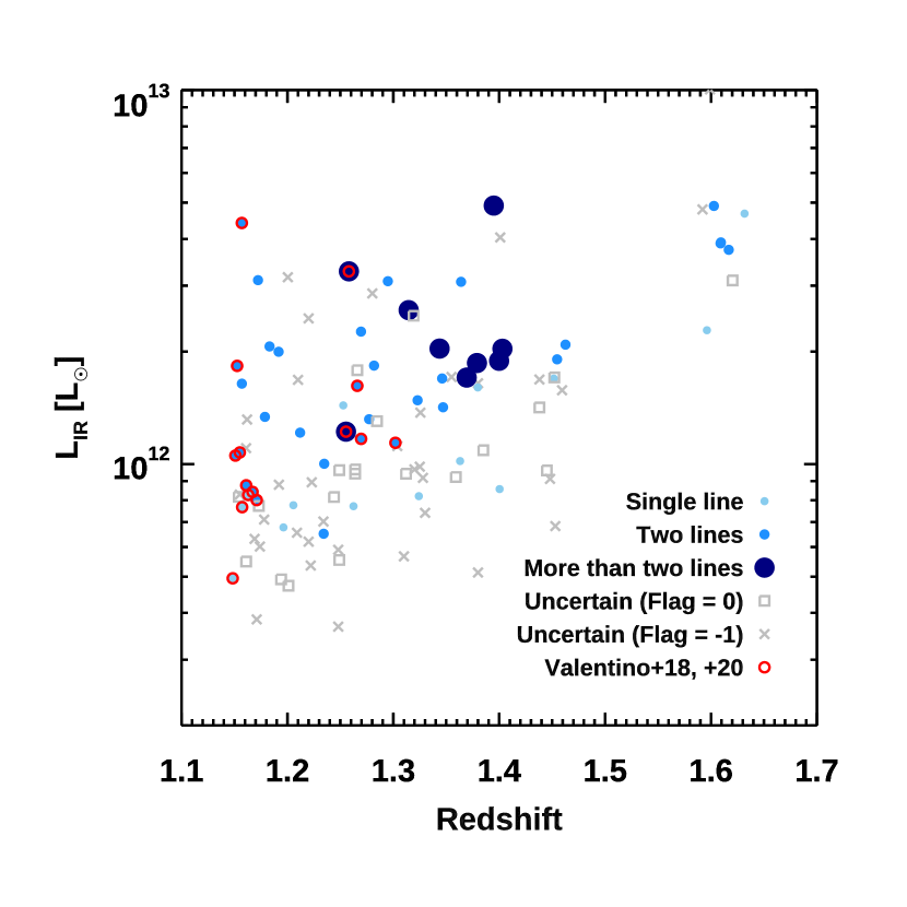
Figure 1: Survey design: the redshifts and total IR luminosities distributions of the primary CO $(5-4)$ sample of our campaign. Gray crosses mark uncertain sources due to poor optical redshifts ($Flag=-1$). Gray open squares indicate uncertain upper limits on every covered line with trustable $z_{\rm spec,opt}$ ($Flag=0$). Light blue, blue, and navy blue filled circles indicate reliable sources with usable information about one, two, or more than two transitions from this work ($Flag\geq 0.5$). Red open circles mark the objects already presented in V18 and V20. Galaxies without an updated far-IR modeling based on the photometry in Jin et al. (2018) are not shown. The flagging classification and the definition of reliable and uncertain data are described in Section 3.2.2.

2 Survey description

Table 1: Summary of the multi-cycle ALMA campaign presented in this work.

Epoch	Band	Transitions	Sample	$\langle t_{\rm int}\rangle$	Beam size	$\langle\mathrm{rms}\rangle$
				[min]		[mJy]
Cycle 3	Band 6	CO $(5-4)$	$123$	$1.6$	$0.8\arcsec$	0.5
Cycle 4	Band 3	CO $(2-1)$	$75$	$4$	$1.4\arcsec$	0.375
Cycle 7	Band 7	CO $(7-6)$, [C I]$(^{3}P_{2}\,-\,^{3}P_{1})$	$15$	$24$	$1.0\arcsec$	$0.25$

2.1 The primary CO $(5-4)$ sample

The survey was originally designed to observe CO $(5-4)$ in a statistical sample of field IR-bright galaxies, distributed on and above the main sequence at $z\simeq 1.1-1.7$ in the COSMOS area (Scoville et al., 2007). The program was prepared for ALMA Cycle 3. The targets had available stellar mass estimates (Muzzin et al., 2013; Laigle et al., 2016), a spectroscopic confirmation from near-IR and optical observations from the COSMOS master catalog (M. Salvato et al. in prep.), and a Herschel/PACS $100$ $\mu$m and/or 160 $\mu$m $3\sigma$ detection in the PEP catalog (Lutz et al., 2011). Initially we considered 178 objects with a predicted CO $(5-4)$ line flux of $I_{54}>1$ Jy km s^-1 over 400 km s^-1, based on the IR luminosity and the $L_{\rm IR}$-$L^{\prime}_{\rm CO(5-4)}$ relation from (Daddi et al., 2015, D15 hereafter). This constant flux cut corresponds to $L_{\rm IR}\gtrsim 10^{12}$ $L_{\odot}$ in the redshift interval under consideration. We then grouped these objects in frequency ranges within ALMA Band 6, allowing for potential individual detections in less than two minutes of on-source integration, while minimizing the overheads. The final spectral sampling includes $123$ primary targets homogeneously spread over the $z$-$L_{\rm IR}$ space (Figure 1), with mean and median stellar masses of $M_{\star}=10^{10.7}\,M_{\odot}$ and a 0.4 dex dispersion. We will refer to these galaxies as the “primary sample” of our survey. Since a new “super-deblended” IR catalog for the COSMOS field became available (Jin et al., 2018), a posteriori we remodeled the SED of each object and updated the initial estimates of $L_{\rm IR}$ (Section 3.3). Twelve targets from the PEP catalog do not have a deblended counterpart in Jin et al. (2018), and, thus, do not have an updated estimate of $L_{\rm IR}$. Moreover, two objects significantly detected in the IR do not have a certain optical counterpart and, thus, a stellar mass estimate. Excluding these sources, based on the new modeling 78 targets lie on the main sequence as parameterized by Sargent et al. (2014) and 31 are classified as starbursts ($\geq 3.5\times$ above the main sequence). The threshold for the definition of starburst is arbitrary and set in order to be consistent with V18 and V20. Five objects have a dominant dusty torus component in the IR SED (see Section 3.3). The final distribution of the targets in the $z$-$L_{\rm IR}$ space with the updated IR modeling is shown in Figure 1. We note that the initial requirement of a PACS detection steered the sample towards upper main-sequence objects and warm dust temperatures $T_{\rm dust}\gtrsim 30$ K.

2.2 The CO $(2-1)$ and CO $(7-6)$ follow-up

The follow-up of the CO $(2-1)$ transition during ALMA Cycle 4 was focused on a subsample of 75/123 objects above a constant line flux threshold of $I_{21}\geq 0.75$ Jy km s^-1. We gathered the potential targets in blocks of frequency settings to contain the overheads, shrinking the initial pool of galaxies with CO $(5-4)$ coverage. Similar considerations apply for the most recent ALMA program in Cycle 7, targeting [C I]$(^{3}P_{2}\,-\,^{3}P_{1})$+CO $(7-6)$ in 15 galaxies with potential simultaneous visibility of [C I]$(^{3}P_{1}\,-\,^{3}P_{0})$. In this case, we sacrificed the flux completeness down to a constant threshold to obtain the largest number of multi-line measurements, adjusting the detection limit of every block of observations to the dimmest source in each pool.

Finally, $15/123$ galaxies have at least a detection of [C I]$(^{3}P_{1}\,-\,^{3}P_{0})$, CO $(4-3)$, [C I]$(^{3}P_{2}\,-\,^{3}P_{1})$, and CO $(7-6)$ from V18 and V20. In the latter, we operated the target selection following a similar strategy as the one outlined here, namely by imposing comparable $L_{\rm IR}$ and redshift cuts. Figure 1 shows the combined information on every targeted line available for the overall sample studied here. We will return to the details of the detection rate below.

3 Data and analysis

3.1 ALMA Observations

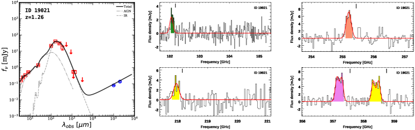
Figure 2: An example of ALMA spectra and far-IR spectral energy distribution. Left: Red open squares and arrows indicate detections and $3\sigma$ upper limits on the IR photometry that we modeled. Blue open circles indicate radio measurements, which we did not include in the fitting. The gray dashed and dotted-dashed lines mark the best-fit Draine & Li (2007) and Mullaney et al. (2011) templates for the star-forming and AGN components, respectively. A stellar template was included when modeling the IRAC bands, but we do not show it to avoid confusion. The black solid line indicates the sum of all the templates. Right: ALMA spectra with detected CO $(2-1)$ (green), CO $(5-4)$ (orange), CO $(7-6)$ (purple), and [C I] (yellow) transitions (CO $(4-3)$ is not available for this source). The solid red line indicates the best-fit Gaussian model. The black tick shows the expected line position based on the optical redshift $z_{\rm spec,opt}$. The full compilation of SEDs and spectra from which we extracted reliable line measurements (Section 3.2.2) is available in the online version of this article.

The primary sample of 123 targets described in Section 2 was observed in Band 6 during ALMA Cycle 3 (#2015.1.00260.S, PI: E. Daddi). The goal of a flux density rms of 0.5 mJy, necessary to detect a line flux of $I_{54}>1$ Jy km s^-1 over $400$ km s^-1at $>5\sigma$, was reached in $\lesssim 1.7$ minutes of integration on source per target (Table 1). The whole program was completed, delivering cubes for all targets with an average beam size of $\sim 0.8\arcsec$. The subsample of 75/123 sources for the CO $(2-1)$ follow-up was observed in Band 3 during ALMA Cycle 4 (#2016.1.00171.S, PI: E. Daddi). With an average on-source integration of $\sim 4$ minutes, the observations matched the requested rms of $0.375$ mJy, allowing us to detect $I_{21}>0.75$ Jy km s^-1 over $400$ km s^-1at $>5\sigma$, in principle. Again, the full program was observed and delivered, providing cubes with an average beam size of $\sim 1.4\arcsec$. Finally, 15/123 galaxies were observed in Band 7 to detect [C I]$(^{3}P_{2}\,-\,^{3}P_{1})$+CO $(7-6)$ during Cycle 7 (#2019.1.01702.S, PI: F. Valentino), reaching a flux density rms of $0.190-0.315$ mJy. We underline that the idea behind this program was to maximize the number of sub-mm line detections per source, rather than reaching a constant flux depth for the whole sample. Thus, the limiting rms of every block of observations was adapted to the faintest object in each group. The final average beam size is $\sim 1.0\arcsec$.

As mentioned in Section 2, 15/123 galaxies in the primary sample have one or multiple detections of the neutral atomic carbon [C I] transitions, CO $(4-3)$, and CO $(7-6)$, as a result of an independent campaign carried out during ALMA Cycle 4 and 6 (#2016.1.01040.S and #2018.1.00635.S, PI: F. Valentino). The delivered Band 6 data have an average beam size of $2.0\times 1\arcsec.7$, reaching a flux threshold of $\sim 0.15$ Jy km s^-1per beam for a line width of $400$ km s^-1(V18). The follow-up in Band 7 reached and $\mathrm{rms}$ of $0.064-0.58$ mJy, and the resulting cubes have an average beam size of $\sim 0.9\arcsec$. We refer the reader to V18 and V20 for more details.

3.2 Data reduction and spectral extraction

We reduced the data following the iterative procedure described in D15 (see also V18, V20, Coogan et al. 2018; Puglisi et al. 2019; Jin et al. 2019 for reference). We calibrated the cubes using the standard pipeline with CASA (McMullin et al., 2007) and analyzed them with customized scripts within GILDAS (Guilloteau & Lucas, 2000). For each source, we combined all the available ALMA observations in the uv space allowing for an arbitrary renormalization of the signal for all tracers. We then modeled each source as circular Gaussian in the uv plane to extract the spectrum, allowing the source position, size, and total flux per channel to vary. Finally, the spectrum was obtained from the fitted total fluxes per channel. This method has no obvious bias against fitting in the image plane (Coogan et al., 2018), but it has more flexibility in fitting parameters. We iteratively looked for spatially extended signal from the $S/N$-weighted combination of all the available tracers, resorting to a point source extraction whenever this search was not successful (D15). In the former case, we could safely measure the size of the emitting source and recover the total flux. When using a point source extraction, we derived upper limits on the sizes and estimated the flux losses as detailed in Appendix A. Finally, we estimated the probability of each galaxy to be unresolved ($P_{\rm unres}$) by comparing the $\chi^{2}$ of the best-fit circular Gaussian and the point source extraction (Puglisi et al., 2019). Using a combination of low- and high-$J$ CO transitions, [C I] lines, and continuum emission, the sizes should be considered as representative of the extension of the molecular gas and cold dust in our galaxies. However, we note that the size is primarily driven by CO $(5-4)$ and its underlying dust continuum emission (see Figure 1 of Puglisi et al., 2019).

3.2.1 Line and continuum flux measurements

We blindly scanned the extracted spectra looking for potential line emission. We did so by looking for the maximum $S/N$ computed over progressively larger frequency windows centered on each channel. The line flux is then the weighted average flux density within the frequency interval maximizing the $S/N$, times the velocity range covered by the channels within the window, and minus the continuum emission. To estimate the latter, we considered a $S/N$-weighted average of line-free channels over the full spectral width ($\sim 7.5$ GHz), assuming an intrinsic power-law shape ($\propto\nu^{3.7}$). The redshift is determined from the weighted mean of the frequencies covered by the candidate line.

To confirm the line emission and avoid noise artifacts, we ran extensive simulations and computed the probability for each candidate line to be spurious ($P_{\rm line}$) following the approach in Jin et al. (2019). The calculation provides the chance that a candidate line with a known $S/N$, frequency, and velocity width appears in the spectrum owing to noise fluctuations, taking into account the full velocity range covered by the observations, the frequency sampling, and assuming a fixed range of acceptable line FWHM. As a further check, two members of our team visually inspected all the available spectra independently.

Once the redshift was determined, we finally remeasured the flux of each line over a fixed velocity width, normally set by CO $(5-4)$ because of its brightness and the widespread availability, being the primary target of our survey. Note that we rounded the velocity width to the closest integer number of channels allowed by the frequency resolution of each spectrum. The adoption of identical apertures for the spectral extractions and constant velocity ranges for the measurements allowed us to derive consistent line ratios and depict meaningful CO SLEDs. We also note that the redshifts and the velocity widths of the detected lines are fully consistent, when they were left free to vary.

For sources without a significant flux detection, we estimated an upper limit around the expected line position. Whenever an alternative ALMA line measurement was available, we adopted $z_{\rm spec,submm}$ and the known velocity width to set a $3\sigma$ limit of $I_{\rm line}>3\times\mathrm{rms_{ch}}\sqrt{dv\Delta v}$, where $\mathrm{rms_{ch}}$ is the average noise per channel over the line velocity width $\Delta v$, and $dv$ is the velocity bin size. Such limits are reliable and useful, given the exact knowledge of the redshift from the sub-mm. When only a $z_{\rm spec,opt}$ was available, we scanned the frequency around the expected location of the line, but eventually measured only upper limits adopting an arbitrary $\Delta v=400$ km s^-1 to be consistent with V18 and V20. Finally, we checked our blind flux measurements against a Gaussian parameterization of the line emission, resulting in a $\sim 10$% flux difference due to the different velocity widths, and fully consistent redshift estimates, similarly to previous works (Coogan et al., 2018, V18). We accounted for this factor by increasing the line fluxes from the spectral scanning by $10$%. We note that a blind scanning is less prone to spurious detections and it provides more reliable estimates, whenever previous detailed knowledge of a source is absent. Therefore, we adopted the fluxes estimated by scanning the spectra as our final measurements.
As an example, we show the spectra of a source with multiple line detections in Figure 2, along with its IR SED. The whole compilation of spectra from which we extracted reliable measurements is available in the online version of this article.

3.2.2 Quality flags and detection rate

We finally classified the spectra and the $z_{\rm spec}$ determination for each line by visual inspection and comparison with the optical/near-IR determination.

• Flag${}_{\rm line}=1$: Secure line measurement due to low probability of being a false positive ($P_{\rm spurious}<0.01$) and/or presence of alternative lines confirming the $z_{\rm spec,submm}$, consistently with the optical/near-IR determination $z_{\rm spec,opt}$.

• Flag${}_{\rm line}=0.5$: Secure upper limit on the line flux, given the presence of alternative sub-mm lines confirming $z_{\rm spec,submm}$.

• Flag${}_{\rm line}=0$: Upper limit on the line flux, assuming a velocity width of $\Delta v=400$ km s^-1centered at the expected frequency based on high-quality $z_{\rm spec,opt}$.

• Flag${}_{\rm line}=-1$: Undetected line and uncertain upper limit due to a poor quality $z_{\rm spec,opt}$.

• Flag${}_{\rm line}=-99$: Line not observed (no data).

We consider “reliable” the flux measurements or upper limits for lines with Flag${}_{\rm line}\geq 0.5$, and “uncertain” when Flag${}_{\rm line}\leq 0$. Adopting this scheme, we recovered 56/123 ($\sim 46$%) sources with “reliable” CO $(5-4)$ flux estimates for the primary sample, and 41/75 ($\sim 55$%) for CO $(2-1)$. As foreseeable for targeted observations, we achieved higher detection rates for CO $(7-6)$ and [C I]$(^{3}P_{2}\,-\,^{3}P_{1})$ (13/15 detections, $\sim 87$%). Considering only sources with previous knowledge of $z_{\rm spec,submm}$ rather than $z_{\rm spec,opt}$, the detection rate jumps to 100%.

In Appendix B we revisit a posteriori the selection of the targets for the CO $(2-1)$ follow-up. This allows us to identify the factors setting the detection rate: the quality of $z_{\rm spec,opt}$, lower $L_{\rm IR}$ than initially estimated, and intrinsically faint lines in bright objects, in order of importance. Here we remark that the imposition of minimum $I_{\mathrm{21}}$ and $I_{\mathrm{54}}$ flux thresholds formally biases their ratio. To account for this selection effect, when deriving average CO SLEDs later on, we will limit the calculation to objects that would have entered the sample of potential CO $(2-1)$ targets according to the revised IR modeling.

3.2.3 Spectroscopic redshift offset: sub-mm vs optical/near-IR

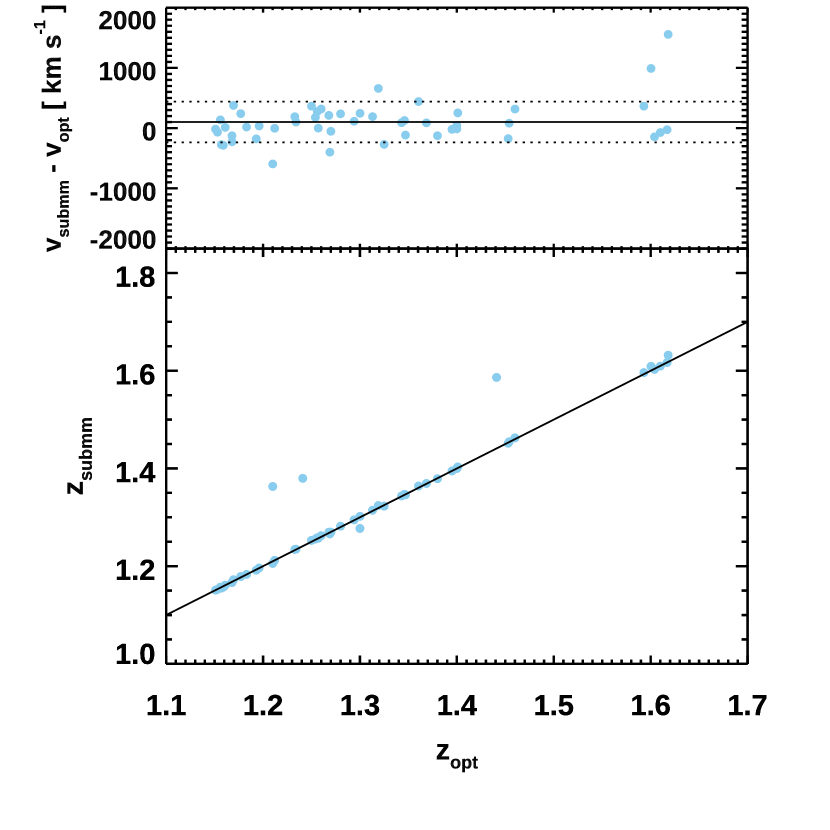
Figure 3: Spectroscopic redshift offset between submillimetric and optical/near-IR observations. Bottom: The blue filled circles indicate the new $z_{\rm spec,submm}$ determinations for trustable emission lines detected by ALMA against the optical/near-IR $z_{\rm spec,opt}$ from the COSMOS master compilation (M. Salvato et al. in prep.). The solid black line mark the locus of $z_{\rm spec,submm}$=$z_{\rm spec,opt}$. Top: $v_{\rm submm}-v_{\rm opt}$ difference as a function of $z_{\rm spec,opt}$, excluding three catastrophic strong outliers and an ascertained misidentification. The solid and dotted lines mark the mean and the $1\sigma$ dispersion of the sample.

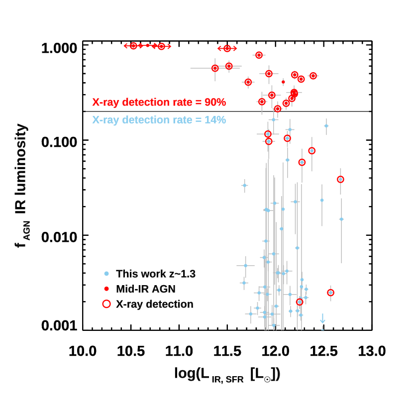
Figure 4: AGN contamination. Fraction of the AGN contribution to the total IR luminosity ($f_{\rm AGN}=L_{\rm IR,AGN}/L_{\rm IR}$) as a function of the IR luminosity from the star-forming component of the SED fitting ($L_{\rm IR,SFR}$). The blue points show the objects with a line emission or an upper limit ($Flag\geq 0$) and a good model of the SED. Red solid circles indicate mid-IR selected AGN. Red empty circles indicate Chandra 2-10 keV detections with $L_{2-10\rm keV}>10^{42}$ erg s^-1. Horizontal red arrows indicate sources with unreliable estimates of $L_{\rm IR,SFR}$ due to the strong AGN contamination.

In Figure 3 we show the comparison between the spectroscopic redshifts for the reliable ALMA sources and their original $z_{\rm spec,opt}$ estimate from the master compilation of the COSMOS field (M. Salvato et al. in prep.). Excluding four sources with ascertained significant deviations ($z_{\rm spec,submm}-z_{\rm spec,opt}>0.05$), the ALMA and the optical/near-IR redshift estimates are in good agreement with mean and median $\left(z_{\rm spec,submm}-z_{\rm spec,opt}\right)<0.001$ and a normalized median absolute deviation (Hoaglin et al., 1983) of $\left|z_{\rm spec,submm}-z_{\rm spec,opt}\right|/(1+z_{\rm spec,submm})=0.001$. The redshift difference corresponds to a mean velocity offset of $\langle\Delta v\mathrm{(submm-opt)}\rangle=101\pm 46$ km s^-1with a dispersion of $338$ km s^-1, as measured over 54 objects. The outliers have either dubious quality or no flags on $z_{\rm spec,opt}$.

3.2.4 Serendipitous detections

We serendipitously found multiple sources in the dust continuum emission maps of 12 primary targets. Four physical pairs are spectroscopically confirmed by ALMA (Puglisi et al., 2019), while the remaining 8/12 are detected in continuum emission only. Five out of 6 reliable systems in this pool are well separated and deblended in both the $K$-band and in the far-IR. We flagged the only other object possibly affected by blending (#51599) and adopted the total stellar mass and $L_{\rm IR}$ as representative of the whole system (see Puglisi et al. 2019 for a possible deblending of this source). We did not include the confirmed deblended companions any further in the analysis, in order to preserve the original selection. However, adding the only object that a posteriori meets our initial criteria would not change the main conclusions of this work.

3.3 Infrared SED modeling

We re-modeled the IR photometry of our sources from the “super-deblended” catalog of the COSMOS field (Jin et al., 2018) in order to derive key physical properties of the sample, notably the total IR luminosity $L_{\rm IR}$, the dust mass $M_{\rm dust}$, and the mean intensity of the radiation field $\langle U\rangle$. Jin et al. (2018) chose radio and UltraVISTA $K_{s}$ priors to deblend the highly confused far-IR and sub-mm images, while performing active removal of non-relevant priors via SED fitting with redshift information and Monte Carlo simulations on real maps, which reduces the degeneracies and results in well-behaved flux density uncertainties (Liu et al., 2018). The catalog includes emission recorded by Spitzer/MIPS at $24$ $\mu$m (Sanders et al., 2007), Herschel/PACS (Lutz et al., 2011) and SPIRE (Oliver et al., 2012) at $100-500$ $\mu$m, JCMT/SCUBA2 at 850 $\mu$m (Geach et al., 2017), ASTE/AzTEC at 1.1 mm (Aretxaga et al., 2011), and IRAM/MAMBO at 1.2 mm (Bertoldi et al., 2007), plus complementary information at VLA/10 cm (3 GHz, Smolčić et al., 2017) and 21 cm (1.4 GHz, Schinnerer et al., 2010). Furthermore, we added to this list the information on the dust continuum emission that we measured with ALMA in the observed $0.8-3.2$ mm range.

Our modeling follows the approach of Magdis et al. (2012) and V20. We used an expanded library of Draine & Li (2007) models and the AGN templates from Mullaney et al. (2011) to estimate the total IR luminosity $L_{\rm IR}(8-1000\,\mu\mathrm{m})$ – splitting the contribution from star-formation and dusty tori –, the dust mass $M_{\rm dust}$, and the intensity of the radiation field $\langle U\rangle$. The latter is a dimensionless quantity that can be written as $\langle U\rangle=1/125\times L_{\rm IR}/M_{\rm dust}$, the constant expressing the power absorbed per unit dust mass in a radiation field where $\langle U\rangle=1$ (Draine & Li, 2007; Magdis et al., 2012). Moreover, $\langle U\rangle$ can be directly related to a mass-weighted dust temperature ($\langle U\rangle=(T_{\rm dust,mass}/18.9\,\mathrm{K})^{6.04}$, Magdis et al. 2017). The mass-weighted $T_{\rm dust,mass}$ is $\sim 10$% lower than the light-weighted estimate (Schreiber et al., 2018).

3.3.1 AGN contamination

Each best-fit IR SED model bears a fraction of the total luminosity due to dusty tori surrounding central AGN: $f_{\rm AGN}=L_{\rm IR,AGN}/L_{\rm IR}$, with $L_{\rm IR}=L_{\rm IR,AGN}+L_{\rm IR,SFR}$. Clearly, the ability to detect the AGN emission critically depends on the coverage of the mid-IR wavelengths and the intrinsic brightness of the dust surrounding the nuclei. We, thus, consider reliably detected the contribution from an AGN when $f_{\mathrm{AGN}}+1\sigma_{f_{\mathrm{AGN}}}\geq 20$%, while galaxies with $f_{\rm AGN}\geq 80$% are flagged as AGN dominated. Estimates of $f_{\mathrm{AGN}}\lesssim 1$% simply indicate the absence of strong AGN components and they should not be taken at face value. For the sake of completeness, in Figure 4 we show their statistical uncertainty $\sigma_{f_{\mathrm{AGN}}}$ associated with the fitting procedure.

According to our scheme, we find AGN signatures in $\sim 30$% of the sample, as previously reported (Puglisi et al., 2019). A similar SED-based classification largely overlaps with Spitzer/IRAC color criteria widely used in the literature (Donley et al., 2012, V20). Figure 4 further shows how our AGN scheme overlaps with the detection rate of hard X-ray photons from Chandra (Marchesi et al., 2016; Civano et al., 2016). Ninety percent of sources with $Flag\geq 0$ and $f_{\rm AGN}+1\sigma_{f_{\mathrm{AGN}}}\geq 20$% also have $L_{\rm 2-10\,keV}\geq 10^{42}$ erg s^-1. This fraction drops to $14$% below the fixed $f_{\rm AGN}$ threshold, which might be considered as the rate of AGN contamination in our star-forming dominated sample. Here we limit the analysis to this classification and to the quantification of the AGN contribution to the total IR luminosity. We note that we will exclude the AGN-dominated galaxies from the rest of the analysis. A specific study of the effects of the AGN on the gas excitation is postponed to the future.

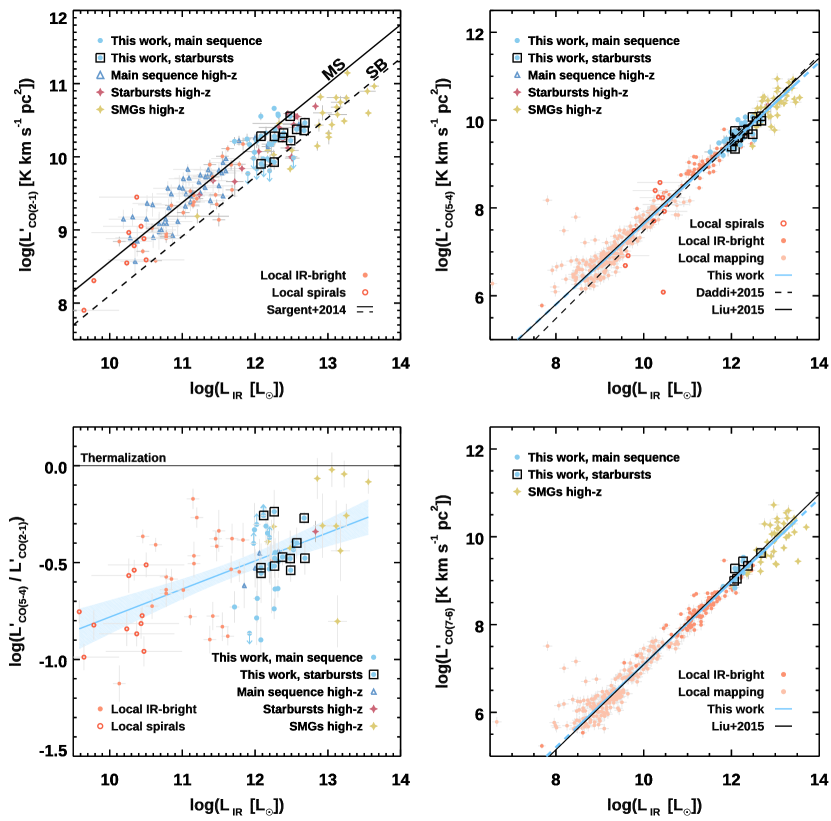
Figure 5: CO – IR luminosities relations. From the top left, clockwise: $L^{\prime}$ [K km s^-1 pc²] luminosities of CO $(2-1)$, CO $(5-4)$, CO $(7-6)$, and the CO $(5-4)$/CO $(2-1)$ ratio as a function of the IR luminosity $L_{\rm IR}$ [$L_{\odot}$]. Symbols are color-coded as labeled (see Section 3.5 for references), where our sample of main sequence and starbursts ($\Delta\mathrm{MS}\geq 3.5$) at $z\sim 1.3$ is marked by blue filled circles and open black squares, respectively. The solid and dashed black lines show the best-fit linear models from previous works (Sargent et al., 2014; Liu et al., 2015a, D15). The blue lines mark our best model, where the dashed segments indicate its extrapolation. The blue shaded area in the bottom left figure shows the 95% confidence interval, omitted in the remaining panels for clarity. The best-fit parameters and the scatter are reported in Table 5. We adopted an extended $L_{\rm IR}$ range in the right panels to show the $L^{\prime}_{\rm CO(5-4)}$ and $L^{\prime}_{\rm CO(7-6)}$ luminosities obtained from mapping nearby objects (Liu et al., 2015a), for which CO $(2-1)$ observations on the same scales are not available. Note that the axes are inverted with respect to the canonical representation of star formation laws.

3.4 Ancillary data

We took advantage of the rich ancillary data and past analysis available for the COSMOS field by compiling stellar masses (Muzzin et al., 2013; Laigle et al., 2016) and optical/near-IR spectroscopic redshifts (M. Salvato et al., in prep.). For sources with X-ray counterparts and a substantial AGN contamination, we refit the UV to near-IR photometry using the code CIGALE (Noll et al., 2009), self-consistently accounting for the presence of emission from the active nuclei across the various bands as detailed in Circosta et al. (2018). While this provided us with a more robust estimate of the stellar masses in presence of strong AGN, we did not find any significant offset between $M_{\star}$ from CIGALE and the COSMOS catalogs for the rest of the sample.

3.5 Literature data

Table 2: CO emission from literature data.

Sample	Transition	References
Herschel-FTS archive	$J=1,2$	K16
	$J=5,7$	L15a
HerCULES	$J=5$	R15, L15a
HERACLES	$J=2,5$	L08; L+in prep.
PHIBSS-2	$J=2$	F19
$BzK$ $z\sim 1.5$	$J=1$	A10; A14
	$J=2$	D10a
	$J=3,5$	Da09, D15
Starburst $z\sim 1.5$	$J=2,3$	S15, S18b;
	$J=5$	S18a
SMGs	various	L15a; V18; V20

To put in context the new ALMA data, we compiled samples from the literature (Table 4). For what concerns objects in the local Universe, we included the local IR-bright galaxies from the full Herschel-FTS archive and their ancillary observations (Liu et al., 2015a; Kamenetzky et al., 2016; Lu et al., 2017, see also V20), covering both low- and high-$J$ CO transitions. We further added the (U)LIRGs from the HerCULES survey (Rosenberg et al., 2015), and the local spirals from the HERACLES (Bigiel et al., 2008; Leroy et al., 2008, 2009) and KINGFISH surveys (Kennicutt et al., 2011; Dale et al., 2012, 2017). We note that other collections of nearby objects with coverage of low-$J$ CO emission are available (e.g., Cicone et al., 2017; Saintonge et al., 2017; Pan et al., 2018; Gao et al., 2019), but we privileged galaxies with observables and properties more directly comparable with our ALMA sample.

Table 3: Scaling relations involving the CO emission lines.

Relation$\dagger$	Slope	Intercept	Intrinsic scatter	Correlation
$x,y$	$\beta$	$\alpha$	$\sigma_{\rm int}$	$\rho$
Luminosities
$L_{\rm IR}$, $L^{\prime}_{\rm CO(5-4)}$	$0.92\pm 0.01$	$-1.55\pm 0.08$	$0.17\pm 0.01$	$0.99$
$L_{\rm IR}$, $L^{\prime}_{\rm CO(7-6)}$	$0.94\pm 0.01$	$-2.34\pm 0.09$	$0.16\pm 0.01$	$0.99$
$L_{\rm IR}$, $R_{52}$	$0.15\pm 0.02$	$-2.23\pm 0.28$	$0.17\pm 0.02$	$0.62$
Distance from the main sequence
$\Delta\mathrm{MS}$, $L^{\prime}_{\rm CO(2-1)}$/$L_{\rm IR}$‡	$-0.34\pm 0.13$	$-1.84\pm 0.08$	$0.24\pm 0.04$	$-0.50$
$\Delta\mathrm{MS}$, $L^{\prime}_{\rm CO(5-4)}$/$L_{\rm IR}$	$-0.01\pm 0.11$	$-2.51\pm 0.07$	$0.33\pm 0.03$	$-0.01$
$\Delta\mathrm{MS}$, $L^{\prime}_{\rm CO(7-6)}$/$L_{\rm IR}$‡	$0.08\pm 0.18$	$-3.02\pm 0.11$	$0.18\pm 0.06$	$0.18$
$\Delta\mathrm{MS}$, $R_{52}$‡	$0.23\pm 0.10$	$-0.64\pm 0.06$	$0.13\pm 0.03$	$0.55$
Drivers of the CO excitation
$\langle U\rangle$, $R_{52}$	$0.36\pm 0.05$	$-0.95\pm 0.07$	$0.15\pm 0.02$	$0.75$
SFE($Z=Z_{\rm FMR}$), $R_{52}$	$0.37\pm 0.05$	$-0.66\pm 0.03$	$0.11\pm 0.03$	$0.88$
SFE($Z=Z_{\odot}$), $R_{52}$	$0.31\pm 0.04$	$-0.68\pm 0.03$	$0.11\pm 0.02$	$0.89$
SFE($Z=Z_{\rm FMR}\lor Z_{\rm super}$), $R_{52}$	$0.32\pm 0.04$	$-0.69\pm 0.03$	$0.12\pm 0.02$	$0.86$
$\Sigma_{\rm SFR}$, $R_{52}$	$0.16\pm 0.02$	$-0.60\pm 0.03$	$0.14\pm 0.02$	$0.82$

At higher redshifts, we incorporated the MS and SB observations from the PHIBSS-2 survey at $z=0.5-0.8$ (Freundlich et al., 2019), the four $BzK$ galaxies in D15 (Dannerbauer et al., 2009; Daddi et al., 2010a; Aravena et al., 2010, 2014), and a pool of starbursts at $z=1.5$ (Silverman et al., 2015, 2018a, 2018b). Finally, we included samples of the high-redshift sub-mm galaxies and quasars (Walter et al., 2011; Alaghband-Zadeh et al., 2013; Aravena et al., 2016; Bothwell et al., 2017; Yang et al., 2017; Andreani et al., 2018; Cañameras et al., 2018; Liu et al., 2015a; Carilli & Walter, 2013, see V18 and V20).

For the whole compilation, we homogenized the measurements to our assumptions (stellar IMF, cosmology, far-IR modeling). Whenever publicly available, we refitted the far-IR photometry adopting the same recipes as described in Section 3.3 to avoid systematics. This is the case for the subsample of the PHIBSS-2 survey in COSMOS and the compilation described in V18 and V20. We used the total $L_{\rm IR}$ reported in Whitaker et al. (2014) for the remaining fields covered by PHIBSS-2. Since a similar approach to ours has been used to model the SED of $BzK$s and SBs at $z\sim 1.5$, we adopted the best-fit values reported in the original papers. As detailed in V20, for the local sample of IR-bright galaxies we converted the IRAS-based $40-400$ $\mu$m far-IR luminosities (Sanders et al., 2003) to total estimates integrated between $8-1000$ $\mu$m as $L_{IR}=1.2\times L_{\rm FIR,\,40-400\,\mu m}$. We calibrated this factor on a subsample of galaxies from the Great Observatories All-Sky LIRGs Survey (GOALS, Armus et al., 2009). Finally, whenever necessary, we increased by a factor of $1.5\times$ the total $L_{\rm IR}$ from the modified black body modeling to match the values from Draine & Li (2007) templates (Magdis et al., 2012).

4 Results

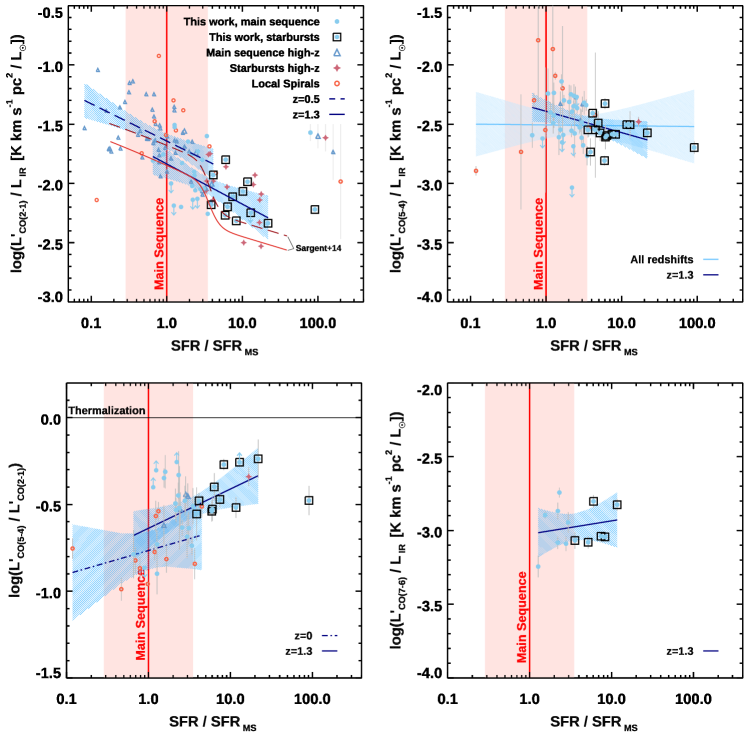
Figure 6: CO emission on and above the main sequence. $L^{\prime}$ [K km s^-1 pc²] / $L_{\rm IR}$ [$L_{\odot}$] for CO $(2-1)$ (top left), CO $(5-4)$ (top right), CO $(7-6)$ (bottom right), and the $L^{\prime}_{\rm CO(5-4)}$/$L^{\prime}_{\rm CO(2-1)}$ ratio (bottom left) as a function of the distance from the main sequence. In every panel, the sample of main sequence galaxies and starbursts at $z\sim 1.3$ presented here is marked by blue filled circles and open black squares. Open blue triangles and purple stars indicate other distant MS galaxies and SBs (at $z=0.5-0.8$ from the PHIBSS-2 survey of CO $(2-1)$, Freundlich et al. 2019; at $z\sim 1.5$ from D15, Silverman et al. 2018a, b). Open red circles signpost local spirals (Leroy et al., 2008; Kennicutt et al., 2011; Dale et al., 2012, 2017, D. Liu et al. in prep.). The red solid line and the shaded area indicate the main sequence within $\|\Delta\mathrm{MS}\|<3.5$ as parameterized by Sargent et al. (2014). The tracks and the shaded areas mark the best-fit models from the linear regression analysis and their 95% confidence interval when modeling the following samples: solid dark blue line: our galaxies at $z\sim 1.3$, excluding the strongest outlier above the main sequence; dashed dark blue line: PHIBSS-2 galaxies at $z=0.5-0.8$; dotted-dashed dark blue line: local spirals; solid light blue line: all samples available (see Table 5 for the parameters). The dashed and solid red lines in the top left panel show the tracks for the two-mode star formation model by Sargent et al. (2014) at $z=0.5$ and $1.5$ and for $M_{\star}=10^{10.7}\,M_{\odot}$, the median mass of both the PHIBSS-2 and our sample. The median error bars for each sample are displayed in the panel.

4.1 How does the CO emission correlate with the infrared luminosity?

In Figure 5 we show how low-, mid-, and high-$J$ CO $L^{\prime}$ luminosities compare with the infrared luminosities $L_{\rm IR}$, including both our new ALMA data on distant main-sequence and starburst galaxies and the literature sample. Note that we inverted the axes with respect to the canonical representation of the star formation laws in order to facilitate the comparison between the various tracers and across different figures. Here we adopted the $L_{\rm IR}$ corrected for the contribution of the dusty tori surrounding the AGN, excluding those sources dominated by such contribution ($f_{\rm AGN}\geq 0.8$, Section 3.3.1) or well-known QSOs at high redshift. These objects tend to increase the scatter of the relation, being overluminous in the mid-IR portion of their SED.

The $L^{\prime}$ luminosity of each CO transition strongly correlates with $L_{\rm IR}$. The upper left panel of Figure 5 shows that the CO $(2-1)$ emission in our main-sequence and starburst galaxies is consistent with the two-mode star formation model described in Sargent et al. (2014), where both samples follow a sub-linear relation with different normalizations ($\mathrm{log}(L^{\prime}_{\mathrm{CO(1-0)}})=0.81\times\mathrm{log}(L_{\rm IR})$, corresponding to a super-linear slope of $1.23$ in the canonical SK plane). Here we applied to the model tracks a $L^{\prime}_{\mathrm{CO(1-0)}}/L^{\prime}_{\mathrm{CO(2-1)}}=1.2$ excitation correction for $BzK$-selected galaxies (Daddi et al., 2010a, D15), but similar considerations hold for the populations of starbursting objects and SMGs.

On the other hand, applying a Bayesian regression analysis (Linmix _err.pro, Kelly 2007):

$$\mathrm{log}\left(\frac{L^{\prime}_{\mathrm{CO,}\,J}}{\mathrm{K\,km\,s^{-1}\,pc^{2}}}\right)=\alpha+\beta\times\mathrm{log}\left(\frac{L_{\rm IR}}{L_{\odot}}\right)$$ (1)

returns $\beta\sim 1$ for both $J=5,7$ (Table 5). Similarly to what is known for local IR-bright and high-redshift SMGs (Greve et al., 2014; Liu et al., 2015a; Lu et al., 2015; Kamenetzky et al., 2016, D15), this proves that mid-/high-$J$ CO luminosities of distant main-sequence and starburst galaxies follow the same tight linear correlation with the total $L_{\rm IR}$, suggesting that these transitions might be used as SFR – rather than molecular $M_{\rm gas}$– tracers. This also suggests caution when deriving the total molecular $M_{\rm gas}$ from high-$J$ CO transitions without prior knowledge of the excitation conditions.

The modeling includes our and literature sources with $L_{\rm IR}\geq 10^{8.5}$ $L_{\odot}$, reliable upper limits on the line luminosities ($Flag=0.5$), uncertainties on both variables, and it excludes AGN-dominated galaxies or QSOs. However, given the large dynamical range spanned by the observations and the small sample of bright QSOs and upper limits, the best-fit models are largely unaffected by their inclusion. The observed points are similarly scattered around the best fit relations for CO $(5-4)$ and CO $(7-6)$, with an intrinsic scatter of $0.16$ dex. We note that excluding the SMGs from the fitting reduces the scatter of the $L_{\rm IR}$-$L^{\prime}_{\rm CO(7-6)}$ relation to $0.14$ dex, but not of the $L_{\rm IR}$-$L^{\prime}_{\rm CO(5-4)}$ correlation, leaving unaltered their slopes. This is consistent with previous determinations of the scatter of the $L^{\prime}_{\rm CO,J}-L_{\rm IR}$ relations based on local IR-bright objects only, which found the $J=7$ luminosity to form the tightest relation with $L_{\rm IR}$ (e.g., Liu et al., 2015a). On the other hand, fitting only the high-redshift samples changes the slopes of the two relations by $<15$% at $<3\sigma$ significance. We note that the inclusion of the low-redshift samples drives the difference between our regression analysis of $L_{\rm IR}$-$L^{\prime}_{\rm CO(5-4)}$ and that of D15.

4.2 CO emission and excitation on and above the main sequence

The homogeneous IR-selection of galaxies presented above allows us to explore the CO emission and the excitation properties over a wide range of distances from the main sequence ($\Delta\mathrm{MS}=\mathrm{SFR/SFR_{\rm MS}}$). This is what is shown in Figure 6, where we report the trend of $L^{\prime}/L_{\rm IR}$ ratios and a proxy for the CO excitation ($R_{52}=$$L^{\prime}_{\rm CO(5-4)}$/$L^{\prime}_{\rm CO(2-1)}$) as a function of the position with respect to the main sequence, parameterized as in Sargent et al. (2014). Here we consider only the dust-obscured SFR traced by $L_{\rm IR}$, without including the contribution from UV emission. The latter becomes of lesser importance in massive SFGs and at increasing redshifts, as for the samples explored here, but this simplification does not apply to local and low $M_{\star}$ objects. We, thus, use galaxy samples with well determined $L_{\rm IR}$ for our comparison.

4.2.1 The low-$J$ transition

The $L^{\prime}_{\rm CO(2-1)}$/$L_{\rm IR}$ ratio constantly declines for increasing $\Delta\mathrm{MS}$, a well-known tendency generally ascribable to the shorter depletion timescales and higher SFEs of starburst galaxies than main-sequence objects (e.g., Daddi et al., 2010b; Tacconi et al., 2010; Genzel et al., 2015; Saintonge et al., 2017; Tacconi et al., 2018; Freundlich et al., 2019; Liu et al., 2019b; Tacconi et al., 2020). A linear regression analysis confirms the existence of a meaningful anticorrelation between $\Delta\mathrm{MS}$ and $L^{\prime}_{\rm CO(2-1)}$/$L_{\rm IR}$ (Figure 6). However, we note that the sub-linear $L_{\rm IR}$-$L^{\prime}_{\rm CO(2-1)}$ relation (Figure 5), coupled with the higher $L_{\rm IR}$ at fixed $M_{\star}$ for distant main-sequence galaxies, introduces a redshift dependence in the $\Delta\mathrm{MS}$-$L^{\prime}_{\rm CO(2-1)}$/$L_{\rm IR}$ relation, which reflects the increasing SFE with redshift (Magdis et al., 2012). The magnitude of this effect in the range $z=0.5-1.5$ covered by the PHIBSS-2 and our sample can be gauged by the shift of the tracks from the two-mode star formation model by Sargent et al. (2014), based on the relations shown in Figure 5. The tracks are calculated for $M_{\star}=10^{10.7}\,M_{\odot}$, the median stellar mass of both samples, and were calibrated against the data available at that time, which did not include a significant population of starbursts. When fitting separately our $z\sim 1.3$ and the PHIBSS-2 samples at $z=0.5-0.8$, we retrieve a similar displacement. The slopes are similar and consistent with the shallow increase of the SFE along the main sequence reported by Sargent et al. (2014), but we do not detect any abrupt change when entering the starburst regime.

4.2.2 The mid-/high-$J$ CO transitions

On the other hand, both the $L^{\prime}_{\rm CO(5-4)}$/$L_{\rm IR}$ and $L^{\prime}_{\rm CO(7-6)}$/$L_{\rm IR}$ ratios are constant as a function of $\Delta\mathrm{MS}$ (Table 5), following the linear $L_{\rm IR}$$-L^{\prime}_{J=5,7}$ correlation shown in Figure 5. This strengthens the idea that mid- and high-$J$ transitions do trace the SFR, rather than the total molecular $M_{\rm gas}$ in galaxies, and they do so independently of their stellar mass and redshift, within the parameter space of massive and metal-rich objects spanned by the observations presented here. Then, the $R_{52}$ ratio naturally rises as the distance from the main sequence increases: the CO emission in starburst galaxies appears more excited than in main-sequence objects at similar stellar masses and redshifts (Table 5). As for $L^{\prime}_{\rm CO(2-1)}$/$L_{\rm IR}$, this relation is expected to evolve with redshift, mimicking the decrease of SFE over cosmic time. A separate fit for the local and the $z\sim 1.3$ galaxies seems to suggest this evolution, even if the small statistics of objects with both CO $(2-1)$ and CO $(5-4)$ lines available, especially on the lower main sequence, makes the $\Delta\mathrm{MS}-R_{52}$ trend more uncertain. The correlations are robust against the exclusion of the strongest outliers (Figure 6). We note that the presence of sources on the MS with large ratios blurs the difference with SBs (see also Puglisi et al., 2019). A diversity of gas excitations conditions even among MS galaxies is evident.

4.3 Main physical drivers of the CO excitation

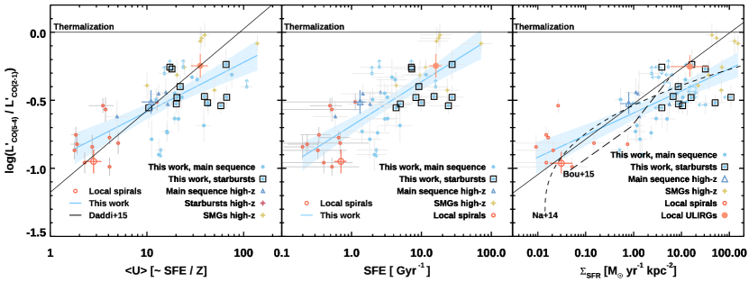
Figure 7: Physical drivers of the CO excitation. $L^{\prime}$ [K km s^-1 pc²] luminosity ratio between CO $(5-4)$ and CO $(2-1)$ as a function of $\langle U\rangle$ from SED modeling (left), SFE (center), and $\Sigma_{\rm SFR}$ (right). Symbols are color-coded as labeled (see Section 3.5 for references), where our sample of main sequence and starbursts at $z\sim 1.3$ is marked by blue filled circles and open black squares, respectively. The solid blue line and the shaded area mark the best-fit model from the linear regression analysis and its 95% confidence interval (see Table 5 for the parameters). The solid black line shows the best-fit model from D15, based on the average values for local spirals, ULIRGs, and $BzK$s at $z=1.5$ (large open red circle, filled red circle, and open blue triangle, respectively). The short- and long-dashed black lines in the right panel indicate the predicted trends from the simulations by Narayanan & Krumholz (2014) and Bournaud et al. (2015), respectively.

We now explore the relation between a proxy of the CO excitation conditions – the $R_{52}$ ratio – and a few physical quantities potentially steering the molecule’s excitation: the star formation efficiency ($\mathrm{SFE=SFR}/M_{\rm gas}$), its combination with the metallicity as probed by the mean interstellar radiation field intensity heating the dust ($\langle U\rangle\propto\mathrm{SFE}/Z$), and the star formation surface density ($\Sigma_{\rm SFR}$, Figure 7). Since we cannot spatially resolve the CO emission in our targets over many beams, this comparison applies to global galaxy scales. By complementing our measurements with the existing literature, we can span a wide interval of redshifts, masses, SFRs, and ISM conditions. The addition of a few tens of main-sequence and starburst galaxies further allows us to derive the average trends among different quantities and to explore their scatter.

4.3.1 The star formation efficiency and the mean interstellar radiation field intensity

By homogeneously modeling the far-IR SEDs of our sample and objects from the literature (Section 3.3), we retrieve sub-linear correlations between $\langle U\rangle$ or SFE and $L^{\prime}_{\rm CO(5-4)}$/$L^{\prime}_{\rm CO(2-1)}$, as previously reported by D15. For our own sample of ALMA detections and reliable upper limits, we calculated SFE by converting the $M_{\rm dust}$ from the SED fitting with Draine & Li (2007) models into $M_{\rm gas}$ applying a metallicity dependent gas-to-dust ratio $\mathrm{log}(\delta_{\rm GDR}(Z))=10.54-0.99\times(12+\mathrm{log(O/H)})$ (Magdis et al., 2012), assuming that galaxies on the main sequence follow a fundamental mass-metallicity relation (FMR, Mannucci et al., 2010). To be consistent with our previous work, we then assumed that starburst galaxies have supersolar metallicities ($\delta_{\rm GDR}\sim 30$, while for reference $\delta_{\rm GDR}\sim 85$ for $Z=Z_{\odot}$, Magdis et al. 2012, see also Puglisi et al. 2017). We factored the 0.2 dex dispersion of the assumed mass-metallicity relation into the uncertainty of SFE. As a consistency check, we also modeled the SFE assuming a $\delta_{\rm GDR}(Z)$ with $Z=Z_{\rm FMR}(M_{\star},\mathrm{SFR})$ and $Z=Z_{\odot}$ for every galaxy in our sample, on and above the main sequence, retrieving consistent results within the uncertainties. We applied the same prescriptions to the literature data, considering SMGs as starbursting galaxies. This exacerbates the differences among observables (or, at least, parameters closer to measurements) when comparing starbursts and main-sequence galaxies. We warn the reader that these are well documented uncertainties on the use of dust as a molecular gas tracer (Magdis et al., 2012; Groves et al., 2015; Scoville et al., 2016), but similar considerations apply to CO and its $\alpha_{\rm CO}$ conversion factor (Bolatto et al., 2013). The choice of using dust instead of CO $(2-1)$ to derive $M_{\rm gas}$ was dictated by the attempt to reduce the correlation with the quantity under scrutiny, $R_{52}$.

The degeneracy on SFE driven by the $\delta_{\rm GDR}$ is partially alleviated when using $\langle U\rangle$ (Figure 7). $\langle U\rangle$ carries similar information to SFE, mapped through an assumption on the metallicity ($\langle U\rangle\propto\mathrm{SFE}/Z$). However, it does not imply an unknown conversion, since $\langle U\rangle\sim L_{\rm IR}/M_{\rm dust}$, while still prone to assumptions as the optical depth of the dust emission (see Section 4.4.5). As clear from Figure 7, starbursts and SMGs tend to display larger $\langle U\rangle$ and CO line ratios than main-sequence galaxies and local spirals, but the distinction in $\langle U\rangle$ is more blurred than in SFE. For reference, we also show the mean location of local spirals, ULIRGs, and $BzK$s at $z\sim 1.5$ from D15. The linear regression analysis in the logarithmic space (Table 5) returns sub-linear trends as in D15, but pointing towards a $1.7\times$ smaller slope and with a larger intrinsic scatter ($0.11-0.15$ dex, Table 5).

4.3.2 The SFR surface density

The right panel of Figure 7 shows the relation between $\Sigma_{\rm SFR}$ and $R_{52}$. For each object, we computed $\Sigma_{\rm SFR}=\mathrm{SFR}/(2\pi R^{2})$, where $R$ is a representative value of the galaxy radius. The latter is rather arbitrary and it depends on the chosen tracer, the depth, resolution, and wavelength of the observations. Here we adopted the ALMA sizes from circular Gaussian fitting for our sample, assuming $R=\mathrm{FWHM}/2$. As mentioned in Section 3.2, this estimate combines all the available lines and continuum measurements, resulting in a size representative of the dust and gas content of each galaxy (Puglisi et al., 2019). We further recomputed the $\Sigma_{\rm SFR}$ for the $BzK$ galaxies in D15, using the Gaussian best-fit results of the rest-frame UV observations to be consistent with our estimates. For the SPT-SMGs, we used the sizes of Spilker et al. (2016), while we employed the 1.4 GHz radio measurements in Liu et al. (2015b) for the local spirals. For reference, we also show the mean values for the $BzK$ galaxies, the local spirals, and ULIRGs as in D15. The best-fit model to the observed points returns a $60$% flatter slope than in D15 (Table 5), but the trends are qualitatively similar. We restate that the choice of the tracer, the resolution, and depth of the observations play a major role in setting the exact values of the slope and intercept in our simple linear model, which should be thus taken with a grain of salt. This is particularly true for spatially resolved local objects, where we attempted to replicate the global, galaxy-scale measurements that can be obtained for distant objects. The observed data points in Figure 7 qualitatively agree with the simulations by Narayanan & Krumholz (2014) and Bournaud et al. (2015), and they support the validity of $\Sigma_{\rm SFR}$ as a good proxy for the gas conditions in galaxies. The total SFR is a worse predictor of the gas excitation conditions (Lu et al., 2014; Kamenetzky et al., 2016), since it does not correlate with the density and temperature probability distribution functions in clouds (Narayanan & Krumholz, 2014). Interestingly, this seems to be partially confirmed by the linear regression analysis we applied here (Table 5): when modeling $R_{52}$ as a function of $L_{\rm IR}$ ($\propto\mathrm{SFR}$, Figure 5) and $\Sigma_{\rm SFR}$, we do find similar slopes, but a larger linear coefficient $\rho$ for $\Sigma_{\rm SFR}$ than for $L_{\rm IR}$. However, $L_{\rm IR}$ alone does correlate with the CO line luminosity ratio.

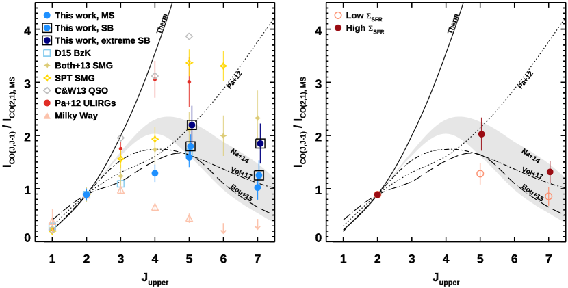
Figure 8: CO excitation ladder. Left: Average CO SLEDs of our samples compared with results from the literature. Each SLED is normalized to the mean CO $(2-1)$ flux of main-sequence galaxies at $z\sim 1.3$. Blue filled circles and open black squares indicate the mean SLEDs of galaxies on the main sequence, starbursts ($\Delta\mathrm{MS}\geq 3.5$), and extreme starbursts ($\Delta\mathrm{MS}\geq 7$), as labeled. The literature samples include the $BzK$ galaxies from D15 (open light blue squares); the average SMGs from Bothwell et al. (2013) (filled green stars) and the SPT-selected ones from Spilker et al. (2014) (open golden stars); high-redshift QSOs from Carilli & Walter (2013) (open gray diamonds); local ULIRGs from Papadopoulos et al. (2012) (red filled circles); the Milky Way from Fixsen et al. (1999) (open pink triangles). The upper limits are at $3\sigma$ significance. The solid line shows the line ratios for a fully thermalized case. The gray shaded area marks the model by Narayanan & Krumholz (2014) for unresolved observations within $\Sigma_{\rm SFR}=1-10\,M_{\odot}\,\mathrm{yr^{-1}\,kpc^{2}}$. The long dashed line indicates the simulations from Bournaud et al. (2015). The dotted line tracks the empirical model by Papadopoulos et al. (2012). The dashed-dotted line points at the analytical model by Vollmer et al. (2017). Right: Mean CO SLEDs for a subsample of objects with detections of CO $(2-1)$, CO $(5-4)$, and estimates of $L_{\rm IR}$ and FIR sizes, split at the median value of $\Sigma_{\rm SFR}$. Light empty and dark filled red circles indicate the low and high $\Sigma_{\rm SFR}$ subsamples. Both SLEDs are normalized to the CO $(2-1)$ flux of the main-sequence sample as in the left panel.

4.4 The CO spectral line energy distribution of distant main-sequence galaxies

Given the large number of galaxies with available and reliable information on CO $(2-1)$ and CO $(5-4)$, in the previous sections we used the ratio of these two lines as a proxy for the CO excitation. However, information of CO $(4-3)$ and CO $(7-6)$ is now available for a subsample of distant main-sequence galaxies, which can be used to constrain their full CO SLED. In Figure 8 we show the average SLEDs for main-sequence and starbursting sources, and we compare them with a selection from the literature, representative of several different galaxy populations. The latter range from the Milky Way (Fixsen et al., 1999) and local ULIRGs (Papadopoulos et al. 2012; see also Lu et al. 2014 and Kamenetzky et al. 2016 for extended libraries of local IR-bright objects), to $BzK$-selected star-forming objects (D15), variously selected high-redshift SMGs (Bothwell et al., 2013; Spilker et al., 2014), and QSOs (Carilli & Walter, 2013). The mean and median $L^{\prime}$ luminosities for our new SLEDs of main-sequence and starburst galaxies, along with their uncertainties, are reported in Table 6. We computed these values for the objects meeting the requirements for a potential CO $(2-1)$ follow-up, based on the updated IR photometry. These galaxies largely overlap with the sample that was effectively observed and reliably characterized (Appendix B) and restraining the analysis to the latter does not affect the results of the following sections, while extending the calculation to all the galaxies with CO $(5-4)$ would artificially decrease the observed ratios. The imposed condition further implies similar $L_{\rm IR}$ for the galaxies entering the analysis. We note that the median $L_{\rm IR}$ for the main-sequence objects with CO $(4-3)$ and [C I]$(^{3}P_{1}\,-\,^{3}P_{0})$ coverage is 0.2 dex smaller than the median value of the galaxies that we consider for the remaining transitions. This might imply an underestimate of the $L^{\prime}_{\rm CO(4-3)}$ and $L^{\prime}_{\mathrm{[C\,\scriptscriptstyle{I}\scriptstyle{]}}^{3}P_{1}\,-\,^{3}P_{0}}$ luminosities by the same factor, for constant $L^{\prime}$/$L_{\rm IR}$ ratios. However, this difference is well within the observed range of ratios (V20) and it does not affect the essence of the results presented in the coming sections.

As in the previous sections, we did not include AGN-dominated objects ($f_{\rm AGN}\geq 80$% of the total $L_{\rm IR}$, Section 3.3.1) in the analysis. A study of their SLEDs and the contribution of X-ray dominated regions (XDR) is postponed to future work. Nevertheless, we remark that the distribution of $f_{\rm AGN}$ is consistent between the samples of main-sequence and the starburst objects analyzed in this Section. For reference and completeness, we show the SLEDs for the subsample with detected CO $(2-1)$ and CO $(5-4)$ in Figure 11 in Appendix C. We show the SLEDs in terms of fluxes to facilitate the comparison with D15, where we normalized all the curves to the mean CO $(2-1)$ line flux of our main-sequence sample. The fluxes are computed at the median redshift of our sample ($z=1.25$), after averaging the luminosities to remove the distance effect.

Table 4: Average emission line luminosities for galaxies at $z\sim 1.25$.

Main-sequence
Transition	$N_{\rm det},N_{\rm up}$	Mean	Median
$L^{\prime}_{\rm CO(2-1)}$	$18,4$	$1.83\pm 0.23$	$1.62^{+0.30}_{-0.70}$
$L^{\prime}_{\rm CO(4-3)}$	$4,0$	$0.66\pm 0.08$	$0.71^{+0.16}_{-0.12}$
$L^{\prime}_{\rm CO(5-4)}$	$20,2$	$0.52\pm 0.06$	$0.44^{+0.26}_{-0.11}$
$L^{\prime}_{\rm CO(7-6)}$	$6,0$	$0.17\pm 0.04$	$0.17^{+0.01}_{-0.06}$
$L^{\prime}_{\mathrm{[C\,\scriptscriptstyle{I}\scriptstyle{]}}^{3}P_{1}\,-\,^{3}P_{0}}$	$7,1$	$0.37\pm 0.05$	$0.31^{+0.09}_{-0.07}$
$L^{\prime}_{\mathrm{[C\,\scriptscriptstyle{I}\scriptstyle{]}}^{3}P_{2}\,-\,^{3}P_{1}}$	$6,0$	$0.17\pm 0.03$	$0.19^{+0.04}_{-0.11}$
Starbursts
Transition	$N_{\rm det},N_{\rm up}$	Mean	Median
$L^{\prime}_{\rm CO(2-1)}$	$11,1$	$1.91\pm 0.24$	$1.90^{+0.38}_{-1.06}$
$L^{\prime}_{\rm CO(4-3)}$	$-$	$-$	$-$
$L^{\prime}_{\rm CO(5-4)}$	$15,0$	$0.62\pm 0.08$	$0.50^{+0.20}_{-0.10}$
$L^{\prime}_{\rm CO(7-6)}$	$6,0$	$0.22\pm 0.05$	$0.22^{+0.06}_{-0.10}$
$L^{\prime}_{\mathrm{[C\,\scriptscriptstyle{I}\scriptstyle{]}}^{3}P_{1}\,-\,^{3}P_{0}}$	$-$	$-$	$-$
$L^{\prime}_{\mathrm{[C\,\scriptscriptstyle{I}\scriptstyle{]}}^{3}P_{2}\,-\,^{3}P_{1}}$	$6,0$	$0.20\pm 0.04$	$0.19^{+0.05}_{-0.08}$
Extreme starbursts
Transition	$N_{\rm det},N_{\rm up}$	Mean	Median
$L^{\prime}_{\rm CO(2-1)}$	$6,1$	$1.80\pm 0.27$	$1.87^{+0.28}_{-1.05}$
$L^{\prime}_{\rm CO(4-3)}$	$-$	$-$	$-$
$L^{\prime}_{\rm CO(5-4)}$	$6,0$	$0.72\pm 0.12$	$0.58^{+0.22}_{-0.13}$
$L^{\prime}_{\rm CO(7-6)}$	$3,0$	$0.31\pm 0.06$	$-$
$L^{\prime}_{\mathrm{[C\,\scriptscriptstyle{I}\scriptstyle{]}}^{3}P_{1}\,-\,^{3}P_{0}}$	$-$	$-$	$-$
$L^{\prime}_{\mathrm{[C\,\scriptscriptstyle{I}\scriptstyle{]}}^{3}P_{2}\,-\,^{3}P_{1}}$	$3,0$	$0.27\pm 0.06$	$-$

4.4.1 CO SLEDs across different galaxy populations

The average SLED for main-sequence galaxies at $z\sim 1.25$ appears significantly more excited than the disk of the Milky Way, but not as excited as local ULIRGs, or high-redshift SMGs and QSOs. Predictably, it is also substantially sub-thermally excited already at mid-$J$ transitions (Dannerbauer et al., 2009). On average, the $R_{52}=L^{\prime}_{\rm CO(5-4)}/L^{\prime}_{\rm CO(2-1)}=I_{\rm CO(5-4)}/I_{\rm CO(2-1)}/(J=5/J=2)^{2}$ ratio for galaxies on the main sequence (Table 7) is $1.8\times$ smaller than ULIRGs (Papadopoulos et al., 2012), $1.3\times$ and $2.1\times$ than SMGs from Bothwell et al. (2013) and Spilker et al. (2014), and $2.4\times$ than distant QSOs (Carilli & Walter, 2013). However, the $R_{52}$ ratio is $3.6\times$ higher than the observed values in the disk of the Milky Way (Fixsen et al., 1999). Similar considerations apply for CO $(7-6)$.

4.4.2 CO SLEDs on and above the main sequence

Table 5: Average line luminosities ratios for galaxies at $z\sim 1.25$.

Transition	Main sequence	Starbursts	Extreme starbursts
$R_{42}$	$0.36\pm 0.06$	$-$	$-$
$R_{52}$	$0.28\pm 0.05$	$0.32\pm 0.06$	$0.40\pm 0.09$
$R_{72}$	$0.09\pm 0.02$	$0.12\pm 0.03$	$0.17\pm 0.04$
$R_{\rm[CI]}$	$0.46\pm 0.10$	$-$	$-$

The excitation of the average SLEDs only tentatively increases with the distance from the main sequence. At mid/high-$J$ transitions, the $L^{\prime}_{J}/L^{\prime}_{\rm CO(2-1)}$ ratios are $1.1\times$ and $1.2\times$ higher for starbursts than main-sequence galaxies for $J=5$ and $7$, respectively (Table 7). This difference and its low significance depend on the threshold for the definition of starbursts, currently set at $\Delta\mathrm{MS}\geq 3.5$; the averaging of all galaxies in only two bins of $\Delta\mathrm{MS}$, further softening the trend shown in Figure 6; and an intrinsic diversity of shapes of CO SLEDs even within a sample of homogeneously selected galaxies (Figure 11). We note that the latter strongly affects any estimate of the molecular gas mass from excited CO transitions.

A more extreme threshold for the starburst regime results in an increase of the deviation between the two samples and of its significance. The difference in $L^{\prime}_{J}/L^{\prime}_{\rm CO(2-1)}$ ratios rises to $1.4\times,1.8\times$ at $J=5,7$ for $\Delta\mathrm{MS}\geq 7$, substantially increasing the CO fluxes for the starbursts and bringing them closer to the typical values of SMGs (Figure 8). The shape also looks flatter, similarly to local IR-bright galaxies (Mashian et al., 2015; Kamenetzky et al., 2016). However, this happens at the expense of the number statistics, which are too sparse for a definitive conclusion about such an extreme definition of starbursts.

The average $R_{52}$ ratio for the IR-selected main-sequence objects is similar to the previous estimate for the four $BzK$-selected galaxies from D15. We note that the addition of the $J=7$ transition constrains the peak of the main-sequence SLED to lower $J$, showing a significant departure from other more extreme populations of galaxies. However, the overall shape of the SLED is flatter than the rapid decrease observed in the disk of the Milky Way, suggesting the existence of a secondary warm component and excluding a steady increase at every $J$ observed so far.

4.4.3 Modeling of the CO SLEDs

The observed SLEDs allow for an assessment of the physically motivated predictions from models and simulations. To simplify the comparison with previous work, in Figure 8 we show the same tracks reported in D15: the empirical model from Papadopoulos et al. (2012) and the hydrodynamical simulations from Narayanan & Krumholz (2014) and Bournaud et al. (2015). Papadopoulos et al. (2012) assumes a hypothetical gas-rich disk with a 10% of the molecular gas in a star-forming phase with Orion A/B-like excitation, along with a quiescent component with an excitation as in the Milky Way. Narayanan & Krumholz (2014) applied a radiative transfer code to simulated discs and mergers to calculate CO SLEDs as a function of $\Sigma_{\rm SFR}$. We adopted their prescription for unresolved observations for galaxies with $\Sigma_{\rm SFR}=1-10\,M_{\odot}\,\mathrm{yr^{-1}\,kpc^{2}}$, which are typical for our main-sequence and starburst galaxies (Figure 7). Bournaud et al. (2015) applied a large velocity gradient model to high-resolution simulations and compute a synthetic CO emission. In particular, they distinguish the high excitation of dense clumpy medium with the less extreme conditions of the diffuse gas. Here we add the analytical model for high-redshift star-forming galaxies by Vollmer et al. (2017). The simulations and the analytical model qualitatively reproduce the rise of the CO SLED of main-sequence objects until mid-$J$ transitions and the following smooth decrease, while the constant rising predicted by Papadopoulos et al. (2012) does not appear to be followed by the average observations. The model by Vollmer et al. (2017) appears to best catch the flat shape at high-$J$, while the simulations from Bournaud et al. (2015) describe well the location of the peak for our samples. The full treatment of the gas physics in simulations and the analytical model seems to capture the main features of the SLEDs of our sample, even if the exact shape and the flux normalizations are partially inconsistent with the observations. However, we warn the reader that the shape of average observed SLEDs is influenced by a mix of galaxies covering a range of excitation conditions, while the modeled profiles are typical of each individual object (at least for the simulations of Bournaud et al. 2015). For a definitive assessment of the various models, it will be critical to extend the coverage to higher-$J$ emission, where their predictions are mostly diverging (see Kamenetzky et al. 2016 and Vollmer et al. 2017 for a discussion about the performances for ULIRGs and SMGs at $J>6$).

4.4.4 Large velocity gradient modeling

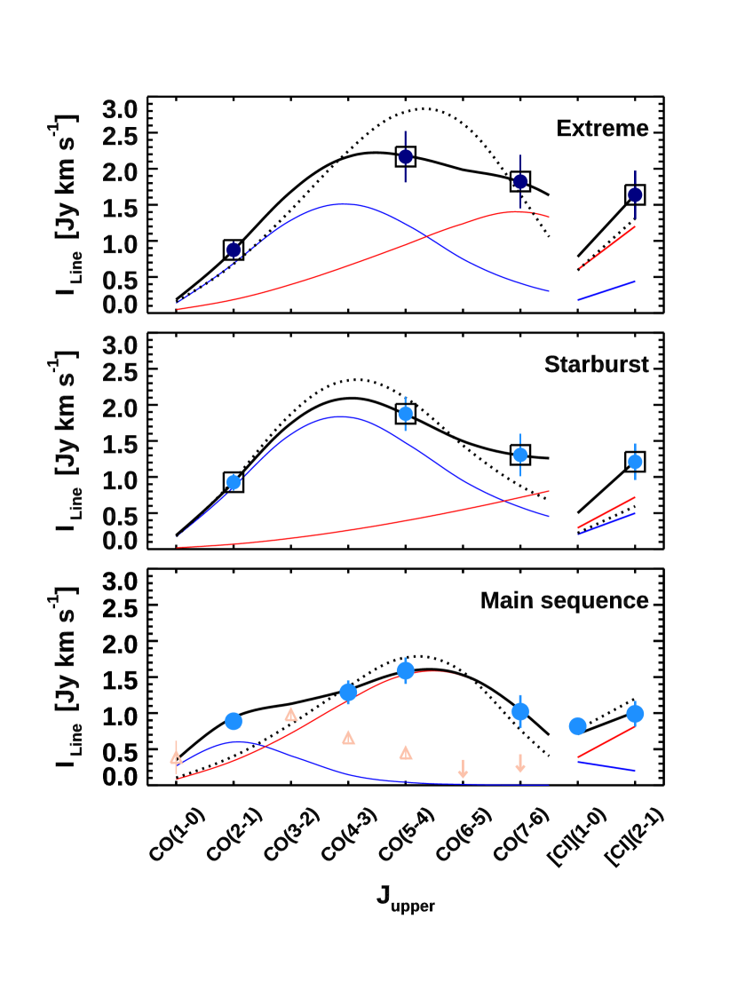
Figure 9: LVG modeling. Large velocity gradient modeling of the observed CO+[C I] SLEDs for main-sequence (bottom panel), starburst ($\Delta\mathrm{MS}\geq 3.5$, central panel), and extreme starburst galaxies ($\Delta\mathrm{MS}\geq 7$, top panel) from our ALMA survey. The filled symbols show the mean fluxes. The blue and red lines show the low- and high-excitation components of the modeling, with the black solid line indicating their sum. The dotted black line shows the best-fit model with a single component. For reference, we show the CO data for the inner disk of the Milky Way (Fixsen et al., 1999) normalized to the CO $(2-1)$ emission of the average main-sequence galaxies as in Figure 8 (pink open triangles). The upper limits are at $3\sigma$ significance.

Large Velocity Gradient (LVG) modeling is a classical approach to gain insight into the properties of the molecular gas in galaxies (Goldreich & Kwan, 1974; Scoville & Solomon, 1974; Young & Scoville, 1991; Papadopoulos & Seaquist, 1998). Here we followed the approach used in D15 (D. Liu et al. in prep.). First, we used the RADEX tool (van der Tak et al., 2007) to create a grid of LVG models. We adopted the collisional rates from Flower (2001) with an ortho-to-para ratio of 3, and a CO abundance to velocity gradient ratio of $[\mathrm{CO/H_{2}}]/(dv/dr)=10^{-5}\,\mathrm{km\,s^{-1}pc^{-1}}$ valid for solar metallicities (Weiß et al., 2005, 2007). We computed a model grid for the median redshift of the sample ($z=1.25$), covering density and temperature intervals of $n(\mathrm{H}_{2})=10^{2}-10^{6}\,\mathrm{cm}^{-3}$ and $T_{\rm kin}=5-300$ K, including the appropriate value of the temperature of the cosmic microwave background. We fixed the line width to $50$ km s^-1 or, equivalently, the cloud scale height to 10 pc, values typical of giant molecular clouds (GMCs). Given the limited amount of information, leaving these parameters or $dv/dr$ free to vary would result in overfitting. Considering that a galaxy contains many of these LVG clouds, the beam filling factor is simply their number. We caution the reader that due to the high degeneracy among the LVG parameters, even with a handful of CO lines one could not obtain results simultaneously constraining $n_{\rm H_{2}}$, $T_{\rm kin}$, and $N(\mathrm{H_{2}})$. Nevertheless, we verified that our estimates of $N(\mathrm{H_{2}})$ and the line optical depths are within the reasonable physical ranges for GMCs (Glover et al., 2015; Tress et al., 2020). All things considered, the best-fit $n_{\rm H_{2}}$ and $T_{\rm kin}$ in this work mostly reflect the relative trends between the different subsamples of main-sequence and starburst galaxies.

We determined the best-fit model via a customized $\chi^{2}$ minimization algorithm, optimized for the exploration of highly multi-dimensional spaces (MICHI2, Liu 2020). In particular, we iteratively sampled the $\chi^{2}$ distribution $15,000$ times, randomizing the parameters within normal distributions centered on the lowest $\chi^{2}$ derived at the previous iteration, but artificially inflating their width. The output consists in best-fit (i.e., $\mathrm{min}(\,\chi^{2})$) parameters and their $\sigma$ uncertainties, plus median and $68\%$ interpercentile values for an arbitrarily large number of components. To better constrain the fit, we further included the [C I] transitions under the assumption that the neutral atomic carbon is co-spatial with CO. We generated the models with RADEX assuming a fixed abundance of $\mathrm{[CI]/H_{2}}=3\times 10^{-5}$ (Weiß et al., 2003; Papadopoulos et al., 2004, but see V18 on the reliability of this assumption). We independently fitted the line fluxes for the average main-sequence and starburst samples (Table 6).

It is evident from Figure 9 that single components do not provide a good representation to the observed CO SLEDs of both populations. This is was already suggested for $BzK$ galaxies (D15, see also Brisbin et al. 2019), and it is a well known fact for local IR-bright galaxies (Papadopoulos et al., 2010b, 2012; Lu et al., 2014; Rosenberg et al., 2015; Kamenetzky et al., 2016) and high-redshift SMGs and QSOs (e.g., Weiß et al., 2007; Aravena et al., 2008; Ivison et al., 2011; Bothwell et al., 2013; Carilli & Walter, 2013; Greve et al., 2014; Spilker et al., 2014; Yang et al., 2017; Cañameras et al., 2018). This result still holds when modeling only the CO emission, excluding the [C I] transitions.

The addition of a second component outperforms the previous attempt. We assumed the existence of a dense and a diffuse phase by imposing that $n_{\rm H_{2},\,low}<n_{\rm H_{2},\,high}$. This results in better constrained densities, but not $T_{\rm kin}$ (Table 9). This is particularly evident for the starbursts, likely due to the lack of mid-$J$ coverage. For both main sequence and starburst galaxies we retrieve the existence of similar low- ($n_{\rm H_{2},\,low}\sim 10^{2}-10^{3}\,\mathrm{cm}^{-3}$) and high-density components ($n_{\rm H_{2},\,high}\sim 10^{4}-10^{6}\,\mathrm{cm}^{-3}$). Furthermore, we retrieve a substantial amount of gas in the dense phase. The latter encloses $\sim 50$% of the total molecular gas mass for main-sequence galaxies. The fraction of denser gas in starbursts is hardly constrained at this stage, possibly due to the absence of lines at $J>7$, where a substantial emission from the excited component might be expected, as shown in local ULIRGs (e.g., Mashian et al., 2015; Kamenetzky et al., 2016) and distant SMGs (e.g., Yang et al., 2017; Cañameras et al., 2018). This is suggested by the flatter shape of the SLEDs for the more extreme starburst with $\Delta\mathrm{MS}\geq 7$. We note that the absolute values of the gas mass from this modeling depend on the adopted CO abundance, constant for both main sequence and starburst galaxies. Therefore, they are subject to the uncertainties already described in Section 4.3.1. Relative comparisons between the two phases for each population still hold, under the assumption that dense and diffuse gas reservoirs share the same metallicity.

Table 6: Best-fit parameters of a double-component LVG modeling of the observed CO+[C I] SLEDs of galaxies at $z\sim 1.25$.

Main-sequence
	Low	High
$\mathrm{log}\left(n_{\rm H_{2}}/[\mathrm{cm^{-3}}]\right)$	$2.2\pm 0.3$	$3.9\pm 0.1$
$T_{\rm kin}/[\mathrm{K}]$	$45\pm 113$	$45\pm 5$
Starburst
	Low	High
$\mathrm{log}\left(n_{\rm H_{2}}/[\mathrm{cm^{-3}}]\right)$	$2.9\pm 0.8$	$6.1\pm 1.4$
$T_{\rm kin}/[\mathrm{K}]$	$300\pm 138$	$75\pm 138$
Extreme starburst
	Low	High
$\mathrm{log}\left(n_{\rm H_{2}}/[\mathrm{cm^{-3}}]\right)$	$3.0\pm 0.8$	$4.5\pm 1.3$
$T_{\rm kin}/[\mathrm{K}]$	$215\pm 138$	$35\pm 138$

4.4.5 The effect of dust opacity on the high-$J$ CO emission

Large dust optical depths even at (sub-)mm wavelengths are responsible for the apparent depressed high-$J$ CO emission in extreme objects as Arp 220 (Greve et al., 2009; Papadopoulos et al., 2010a; Rangwala et al., 2011; Scoville et al., 2017b). This is due to the fact that for $\tau_{\rm dust}\gg 1$, the line emissions are largely erased by the quasi-black body dust continuum (Papadopoulos et al., 2010a). A modeling of the dust continuum emission leaving the optical depth free to vary can provide meaningful results only when the SED is well sampled from mid-IR to mm wavelengths, and it might still return degenerate solutions with the temperature $T_{\rm dust}$, in absence of independent ways to distinguish them (Cortzen et al., 2020). Indeed, our SED modeling is based on the assumption that the dust emission is optically thin above $100\,\mu\mathrm{m}$.

Here we tested our assumption by computing the dust optical depth at the CO $(5-4)$ and CO $(7-6)$ wavelengths as $\tau_{\rm dust}=\kappa(\nu)\,\Sigma_{d}=\kappa_{\rm 850\,\mu m}\,(\nu/\nu_{\rm 850\,\mu m})^{\,\beta}\,M_{\rm dust}/(2\pi R^{2})$, where $\kappa$ is the frequency-dependent dust opacity, and $\Sigma_{d}$ the dust mass surface density (e.g., Casey et al., 2014). We adopted $\kappa_{\rm 850\,\mu m}=0.43\,\mathrm{cm^{-2}g^{-1}}$ and $\beta=2$ (Li & Draine, 2001), the $M_{\rm dust}$ from the SED modeling (Section 3.3), and the sizes from the ALMA measurements. We note that, while using one of the outputs of the SED fitting, this sanity check is not tautological, given the introduction of the size in the calculation. For sources with a significant CO $(5-4)$ line detection, a determination of $M_{\rm dust}$ and of the size from ALMA, we retrieve $\langle\tau_{\rm dust}\,(520\mu\mathrm{m})_{\rm CO(5-4)}\rangle=0.012\pm 0.003$, including the lower limits on $\tau_{\rm dust}$ due to the upper limits on the sizes. For the dust continuum emission under CO $(7-6)$, we find $\langle\tau_{\rm dust}\,(371\mu\mathrm{m})_{\rm CO(7-6)}\rangle=0.020\pm 0.007$, with a maximum of $0.08$, where all the CO $(7-6)$ detections have a safe determination of their size. We note that the same calculation with $M_{\rm dust}$ derived from an ideal SED modeling with the opacity as a free parameter would be lower, further decreasing the value of $\tau_{\rm dust}$.

The largest opacities are associated with strongly starbursting galaxies and/or AGN contamination, but their observed high-$J$/low-$J$ CO ratios do not appear systematically depressed compared to the rest of the sample. However, they do have $\tau_{\rm dust}=1$ for rest-frame $\lambda\sim 100-140$ $\mu$m, similar to several high-redshift SMGs and indicating that their $M_{\rm dust}$ are likely overestimated and $T_{\rm dust}$ cooler than what they really are (Jin et al., 2019; Cortzen et al., 2020). These cases represent $<5$% of the sample for which we could carry out the test on the opacity, and they do not influence the final results. Therefore, it appears that the dust opacity does not have a significant impact on the emission of mid- and high-$J$ CO lines on galaxy scales in our sample, and this is due to the less extreme $\Sigma_{\rm dust}$ compared to, e.g., the one of Arp 220. However, we notice that this is a point to be reassessed with higher spatial resolution measurements, which might well reveal compact pockets of gas within our targets more affected by the dust absorption.

5 Discussion

In the previous sections, we showed that, on global scales, the CO line emission and excitation of main sequence and starburst galaxies broadly correlate with a variety of properties. The high-$J$ CO line luminosities ($J=5,7$) are quasi-linearly related to the star formation rate, suggesting a physical connection with the gas pockets where new stars are formed. The low-$J$ CO line emission is associated with less dense molecular gas, tracing the bulk of its mass in galaxies. Interestingly, the $L^{\prime}_{\rm CO(5-4)}$/$L^{\prime}_{\rm CO(2-1)}$ ratio and overall CO SLED increase as a function of the total infrared luminosity $L_{\rm IR}$ ($\propto\mathrm{SFR}$), the mean intensity of the radiation field heating up the dust $\langle U\rangle$ ($\propto T_{\rm dust}$), the star formation efficiency $\mathrm{SFE}=\mathrm{SFR}/M_{\star}$, the density of the SFR ($\Sigma_{\rm SFR}$), and, less distinctly, with the distance from the main sequence $\Delta\mathrm{MS}$. A comparison of the strength of the observed correlations and their intrinsic scatter (Table 5) offers further insight into this network of properties.

5.1 The spatial distribution of SFR as the driver of the properties of star-forming galaxies

The main physical driver of the CO excitation seems to be a combination of the amount of star formation occurring in the galaxy and its spatial distribution. While a SFR-$R_{52}$ correlation does exist, its strength increases by using $\Sigma_{\rm SFR}$, instead. This naturally follows the fact that dense gas concentrations ignite more compact star-forming regions, producing large UV radiation fields and cosmic ray rates, and warming up the dust (Narayanan & Krumholz, 2014). This is reflected on the similarly strong and tight $\langle U\rangle$-$R_{52}$ relation, and on the enhancement of the excitation as a function of the SFE, boosted in more compact gas configurations (Papadopoulos et al., 2012). Note that the correlation between the CO excitation and $\langle U\rangle$ does not necessarily imply that the interstellar radiation field is responsible for the excitation of the mid-/high-$J$ transitions. If multi-component PDRs have been shown to be sufficient to describe the CO SLED of local spirals (Rigopoulou et al., 2013), this is not the case for starbursts where mechanical heating induced by SF-related (supernovae) or unrelated (mergers, AGN outflows, radio-jets) shocks are invoked to explain the observations (Rangwala et al. 2011; Kamenetzky et al. 2012; Lu et al. 2014; Kamenetzky et al. 2016; see Brisbin et al. 2019 for the case of a distant main-sequence galaxy). The correlation with $\langle U\rangle$ would then be indirect: it is the stellar feedback from the intense star formation to drive it (Wu et al., 2015). This might well be the case for the most extreme starbursts, for which PDRs cannot reproduce the observed flat CO SLEDs (Kamenetzky et al., 2016). We note that the models in Figure 8 specifically contemplating a recipe for the mechanical heating from SNae better reproduce the flat shapes of the CO SLEDs and the location of their peaks (Bournaud et al. 2015; Vollmer et al. 2017, and see the discussion in Papadopoulos et al. 2012).

The global rise of $R_{52}$ with the distance from the main sequence can be interpreted considering that $\Sigma_{\rm SFR}$ overall increases with $\Delta\mathrm{MS}$ (Elbaz et al., 2011). Moreover, the high gas fractions inducing clumping in turbulent high-redshift massive disks further enhance this effect (Bournaud et al., 2015), increasing the level of CO excitation of distant main-sequence galaxies with respect to local Milky Way-like objects. In other words, the same mechanisms that we consider here as acting on global galaxy scales might well be in action in sub-galactic massive clumps, effectively mimicking starburst environments (Zanella et al., 2015, 2019). This is also consistent with the results from LVG modeling, where the density of the collisionally excited gas is the term driving the high-$J$ emission, given the fast de-excitation rates. Finally, taken to its extreme consequences, the formation of hundreds or even thousands of stars per kpc² and the ensuing massive layers of dust surrounding them (e.g., Arp 220, Barcos-Muñoz et al., 2015; Scoville et al., 2017b) affects the emerging CO spectrum of a galaxy, inducing the uttermost opacities at long wavelengths (e.g., Blain et al., 2003; Greve et al., 2009; Riechers et al., 2013; Huang et al., 2014; Lutz et al., 2016; Hodge et al., 2016; Spilker et al., 2016; Simpson et al., 2017), reducing the apparent CO excitation at high-$J$ (Papadopoulos et al., 2010a; Rangwala et al., 2011) and the dust temperature, affecting the dust mass estimates if not properly taken into account (Jin et al., 2019; Cortzen et al., 2020).

5.2 What is a starburst?

The scenario presented above has been formulated in various flavors to individually explain several of the properties reported here. The main addition of this work, namely the excitation of CO in distant main-sequence and starburst galaxies, fits in the general picture that we sketched. The ensemble of properties and correlations we reported here can also be used to revisit the definition of what a “starburst” is. A standard operational classification is based on the distance from the observed empirical $M_{\star}$-SFR correlation, the main sequence. This proved to be a useful distinction and an excellent predictor of several trends (e.g., Sargent et al., 2014), but recent results, including our present and previous analysis (Puglisi et al., 2019), show that the demarcation between starburst and main sequence galaxies is more blurred that we previously considered. We do find “starburst-like” behaviors on the main sequence (Elbaz et al., 2018), likely linked to the existence of transitional objects (Popping et al., 2017; Barro et al., 2017b; Gómez-Guijarro et al., 2019; Puglisi et al., 2019, A. Puglisi et al. in prep., to limit the references to recent works based on sub-mm observations). Such transition might well imply an imminent increase of the SFR, driving the object in the realm of starbursts (e.g., Barro et al., 2017b), or its cessation, bringing the system back onto or even below the main sequence (Gómez-Guijarro et al., 2019; Puglisi et al., 2019), with the CO properties potentially able to distinguish between these two scenarios. Regardless of these transitional objects, a definition of starburst based on $\Sigma_{\rm SFR}$, rather than $\Delta\mathrm{MS}$, would naturally better account for the observed molecular gas excitation properties, dust temperatures and opacities, or SFE (see also Elbaz et al., 2011; Rujopakarn et al., 2011; Jiménez-Andrade et al., 2018; Tacconi et al., 2020). As an example, in Figure 8 we show the mean SLED of the subsample of galaxies with both CO $(2-1)$ and CO $(5-4)$ coverage, split at its median $\Sigma_{\rm SFR}$. While only tentative at this stage, this suggests a trend of increasing CO excitation with $\Sigma_{\rm SFR}$, consistently with Figure 7 and what mentioned above.

In more physical terms, the new definition would trace the observed correlations back to a common origin: the accumulation of gas and formation of stars in compact configurations, following global or local dynamical changes in the galaxy structure. The latter might be due to major mergers, known to be primary drivers of starbursts activity in the local Universe (Sanders & Mirabel, 1996), or in presence of higher gas fractions, to minor mergers (Bustamante et al., 2018; Gómez-Guijarro et al., 2018) or violent disk instabilities induced by a sudden alteration of the gravitational equilibrium, particularly effective at high redshift (e.g., Bournaud et al., 2007; Ceverino et al., 2010; Dekel & Burkert, 2014). Such gas concentrations would further increase the AGN activity (Elbaz et al., 2018), spread also in our sample. Moreover, a definition based on $\Sigma_{\rm SFR}$ would allow for the classification of SMGs, normally hard to achieve because of the lack of $M_{\star}$ determinations, potentially sorting extended massive disks (Hodge et al., 2016, 2019), and bona fide ongoing gas-rich mergers (see Casey et al., 2014, for a review of current models for the formation of dusty star-forming galaxies). We will explore the detailed properties of our sample as a function of size and compactness in a dedicated work (A. Puglisi et al. in prep.).

6 Conclusions

We presented the outcome of a multi-cycle ALMA survey of the CO emission in IR-selected galaxies on and above the main sequence at $z\sim 1.3$. We obtained new observations of low- to high-$J$ lines that we complemented with existing samples of local and distant star-forming galaxies. In detail:

1. We report new detections of CO $(5-4)$, CO $(2-1)$, and CO $(7-6)$(+[C I]$(^{3}P_{2}\,-\,^{3}P_{1})$) for 50, 33, and 13 galaxies, respectively, corresponding to detection rates of $\sim 50-80$%.

2. We found that the CO $(5-4)$ and CO $(7-6)$ luminosities of both main-sequence and starburst galaxies follow an almost linear and tight ($\sigma_{\rm int}=0.16$ dex) correlation with the total $L_{\rm IR}$, as previously established for local IR-bright galaxies, spirals, and distant SMGs. On the other hand, the CO $(2-1)$ emission of main sequence and starburst is consistent with the integrated SK law. This suggests that the CO $(5-4)$ and CO $(7-6)$ emission is associated with the reservoirs of actively star-forming gas in galaxies, while CO $(2-1)$ traces the total mass of cold and less dense molecular medium. This also suggests caution when deriving the total molecular $M_{\rm gas}$ from high-$J$ CO transitions.

3. Moreover, we found the CO $(2-1)$/$L_{\rm IR}$ ratio to steadily decrease as a function of the distance from the main sequence $\Delta\mathrm{MS}$, while CO $(5-4)$/$L_{\rm IR}$ and CO $(7-6)$/$L_{\rm IR}$ remain constant. This further supports the idea that mid- and high-$J$ transitions trace the SFR, independently of their stellar mass and redshift, within the parameter space spanned by our observations.

4. We derived monotonically increasing CO $(5-4)$/CO $(2-1)$ luminosity ratios – a proxy for the CO excitation – as a function of increasing star formation efficiency, mean intensity radiation field $\langle U\rangle$, SFR surface density $\Sigma_{\rm SFR}$, and, less distinctly, $\Delta\mathrm{MS}$.

5. We found the overall CO SLED of distant main-sequence galaxies up to CO $(7-6)$ to be more excited than the disk of the Milky Way, but less than local ULIRGs or high-redshift SMGs and QSOs. An intrinsic variety of shapes is present, as shown by the dispersion of the observed CO luminosity ratios, blurring the distinction between the SLEDs of starbursts and upper main-sequence objects. The dust opacity does not appear to significantly suppress the high-$J$ CO emission even for the most extreme objects in our sample, due to relatively low dust mass surface densities compared to, e.g., Arp 220, the prototypical case for this matter. However, this has to be further tested with observations at higher spatial resolution.

6. We modeled the observed CO(+[C I]) SLEDs adopting the LVG method. The addition of high-$J$ CO and [C I] lines indicates the existence of a second highly excited component both for starbursts and main-sequence galaxies, similarly to what invoked to explain the SLEDs of local ULIRGs and SMGs. Imposing the existence of a dense and a diffuse component, we retrieve substantial amount of gas in the former phase ($n_{\rm H_{2},\,high}\sim 10^{4}-10^{5}$ cm^-3), contributing to $\sim 50$% of the total molecular gas mass for main-sequence galaxies.

7. We interpret the CO excitation conditions as driven by the combination of large SFRs over compact regions. Such large $\Sigma_{\rm SFR}$ values naturally explain the large gas densities and high temperatures due to increased UV radiation fields, cosmic ray heating, and dust and gas coupling. Larger densities also naturally induce enhanced SFEs, as canonically advocated for starbursts. An operational definition based on $\Sigma_{\rm SFR}$ rather than on the offset from the main sequence might better separate truly starbursting galaxies from secularly evolving disks.

8. Idealized simulations, analytical, and semi-empirical models qualitatively account for the increase of the CO excitation in distant main-sequence and starburst galaxies peaking around $J\sim 4-5$, but starting from different premises and resulting in shapes and normalizations partially inconsistent with the average observed trends. The addition of transitions at $J>7$ will be the key for a definitive assessments of several models.

Appendix A Total recovered fluxes

The total flux of a source can be robustly recovered if its size is securely estimated. However, our iterative extraction could drive to flux losses when we estimate only an upper limit on the size, and such value is comparable with the beam size. We estimated these losses as detailed in Appendix B of V20, namely by injecting artificial bright galaxies with circular Gaussian profiles and a FWHM fixed to the $1\sigma$ upper limit on the size in the uv plane, and then re-extracting their fluxes with the fiducial point source profile. We then corrected the extracted fluxes to ($I_{\rm Gauss}/I_{\rm Point}+1)/2$ and added in quadrature the absolute error on such correction ($\sigma_{\rm corr}=(I_{\rm Gauss}-I_{\rm Point})/2$) to the statistical uncertainty. The correction does not depend on the brightness of the injected mock source, provided that it is significantly detected ($\mathrm{SN}\geq 10$), nor on its position in the map. The sizes and the flux corrections are reported in the data release.

Appendix B Revisiting the target selection a posteriori

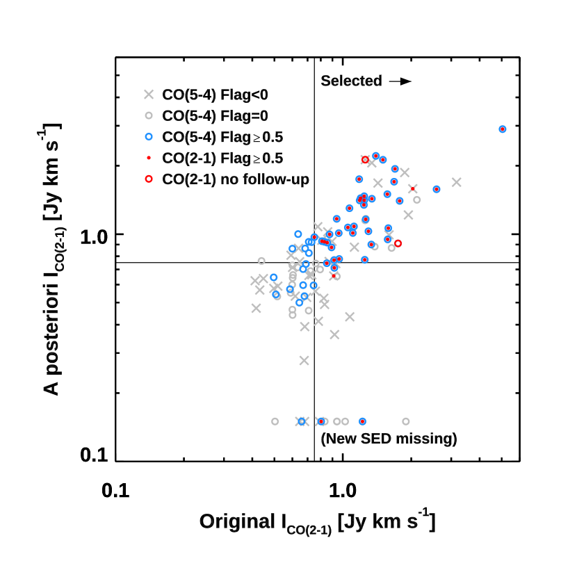
Figure 10: Revisiting the selection and the impact on the detection rate. Predicted $I_{\mathrm{21}}$ fluxes with the original $L_{\rm IR}$ based on PACS detections and on the new IR photometry from Jin et al. (2018). The symbols mark the whole parent sample of 123 galaxies with ALMA Band 6 observations targeting CO $(5-4)$. Gray crosses, gray open circles, and blue open circles indicate sources with uncertain and reliable information on CO $(5-4)$ ($Flag<0,\,0,\,\geq 0.5$, respectively, Section 3.2.2). Red filled circles show galaxies with reliable information on CO $(2-1)$ ($Flag\geq 0.5$). Open red circles mark objects with predicted fluxes bright enough to be observed according to both the initial and the revised SED modeling, but that did not enter the final selection due to the frequency grouping. The black solid lines indicate the depth of the ALMA Band 3 observations: objects on the right side of the vertical line were selected for the follow-up (excluding the red open circles); object above the horizontal line could have been selected, if the updated photometry were available when preparing the observations. Objects with missing photometry in Jin et al. (2018) are artificially set to $I_{\rm CO(2-1)}=0.15$ Jy km s^-1 and labeled accordingly.

Reconstructing a posteriori the target selection for the CO $(2-1)$ follow-up observations, with the improved constraints on the IR photometry that became available in the meantime, allows us to get a handle on the factors determining the detection rates described in Section 3.2.2. In Figure 10, we show the original prediction of the $I_{\rm CO(2-1)}^{\rm pred}$ fluxes computed from previous $L_{\rm IR}$ estimates from the PEP survey (Section 2), against an updated version based on the far-IR modeling of the deblended photometry from Jin et al. (2018). Excluding 12 sources from the PEP survey without a counterpart in the deblended catalog, the flux predictions scatter around the one-to-one relation. Galaxies in the bottom right quadrant of Figure 10 were bright enough to be selected for the follow-up observations, but they would have missed the cut based on the updated $L_{\rm IR}$. The negligible fraction of CO $(2-1)$ detections among these objects supports the hypothesis that they are indeed too faint to be detected at the current depth. On the other hand, for the sources in the top right quadrant of Figure 10, the new photometric modeling supports the initial selection. In fact, this is where virtually all CO $(2-1)$ detections are located. Undetected objects primarily lack reliable information of CO $(5-4)$ and have low quality flags on the optical/near-IR spectroscopic redshifts $z_{\rm spec,opt}$. Only a minor fraction of IR-bright sources do have secure $z_{\rm spec,opt}$, but remained undetected in CO $(5-4)$ and CO $(2-1)$, likely due to bona fide dimmer line fluxes than predicted. Galaxies in the remaining left quadrants were not selected for the CO $(2-1)$ follow-up and their CO $(5-4)$ detection rate is set by a combination of bad $z_{\rm spec,opt}$, lower $L_{\rm IR}$ than previously estimated, and intrinsically faint lines in bright objects, in order of importance. The latter are physically interesting, but we cannot currently put any constraints on their properties, in absence of a secure $z_{\rm spec,submm}$.

Appendix C The diversity of the CO SLEDs of galaxies on and above the main sequence

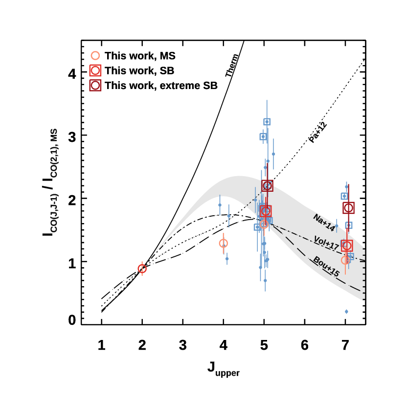
Figure 11: Diversity of CO SLEDs for main-sequence and starburst galaxies. Blue filled circles and open squares indicate the main-sequence and starburst galaxies with detected CO $(5-4)$ and CO $(2-1)$ lines from our ALMA follow-up, normalized to the mean CO $(2-1)$ flux for the main-sequence sample. The open red circles and squares indicate the mean fluxes for main-sequence, starburst ($\Delta\mathrm{MS}\geq 3.5$), and extreme starburst ($\Delta\mathrm{MS}\geq 7$) objects. The solid line shows the line ratios for a fully thermalized case. The gray shaded area marks the model by Narayanan & Krumholz (2014) for unresolved observations within $\Sigma_{\rm SFR}=1-10\,M_{\odot}\,\mathrm{yr^{-1}\,kpc^{2}}$. The long dashed line indicates the simulations from Bournaud et al. (2015). The dotted line tracks the empirical model by Papadopoulos et al. (2012). The dashed-dotted line points at the analytical model by Vollmer et al. (2017).

In Figure 11 we show the CO SLEDs for the subsample of main-sequence and starburst galaxies with CO $(2-1)$ and CO $(5-4)$ detections from our ALMA observations, normalized to the mean CO $(2-1)$ flux for the main-sequence sample (Section 4.4). This figure highlights the variety of shapes displayed even by a homogeneously selected sample of normal and extreme galaxies at high redshift.

Appendix D Data tables, galaxy spectra and spectral energy distribution

Figure 2 shows an example of the ALMA spectra and the IR SED for our sample of reliable sources used in the analysis ($Flag\geq 0.5$). The whole compilation of spectra from which we extracted reliable information is available in the online version of the article. Similarly, the full data table is made public in .fits format. The description of the columns is listed in Table 10.

Table 7: Column description for the data release.

Name	Units	Description
ID	…	Identifier
R.A.	hh:mm:ss	Right ascension
Dec	dd:mm:ss	Declination
zspec_opticalnir	…	Optical/near-IR spectroscopic redshift (M. Salvato et al., in prep.)
(d)zspec_submm	…	ALMA sub-mm spectroscopic redshift
Log_StellarMass	$M_{\odot}$	Logarithm of the stellar mass (Chabrier 2003 IMF)
(d)Total_LIR	$L_{\odot}$	Total $8-1000$ $\mu$m $L_{\rm IR}$ (Draine & Li 2007; Mullaney et al. 2011)
(d)SF_LIR	$L_{\odot}$	$L_{\rm IR,\,SFR}$ from the star-forming component ($L_{\rm IR,\,SFR}=L_{\rm IR}-L_{\rm IR,\,AGN}$)
(d)AGN_LIR	$L_{\odot}$	$L_{\rm IR,\,AGN}$ from the AGN component ($L_{\rm IR,\,AGN}=L_{\rm IR}\times f_{\rm AGN})$
(d)$f_{\rm AGN}$	…	Fraction of $L_{\rm IR}$ due to the AGN emission
(d)$M_{\rm dust}$	$M_{\odot}$	Dust mass (Draine & Li 2007)
(d)$U$	…	Mean intensity of the interstellar radiation field (Draine & Li 2007)
DistanceMS	…	Distance from the main sequence as parameterized in Sargent et al. (2014)
(d)Size	arcsec	Source angular size from ALMA
OneSigma_Size	arcsec	$1\sigma$ upper limit on the source angular size from ALMA
Probability_Unresolved		Probability of being unresolved (Puglisi et al. 2019)
Flux_Line($X$)	Jy km s-1	Velocity integrated flux of line $X$
SNR_($X$)	…	Signal to noise ratio of the flux of line $X$
OneSigma_($X$)	Jy km s-1	$1\sigma$ upper limit on the flux of line $X$
Width_($X$)	km s-1	Velocity width of line $X$
(d)ApertureCorr_($X$)	…	Aperture correction for line $X$
Prob_Line($X$)	…	Probability of spurious detection of line $X$
Flag_($X$)	…	Quality and usage flag for line $X$
FreqContinuumBand($B$)_($X$)	GHz	Frequency in Band $B$ under line $X$ for the estimate of the continuum emission
(d)ContinuumBand($B$)_($X$)	mJy	Continuum emission in Band $B$ under line $X$