The scalar sunset diagram at finite temperature
with imaginary square masses

Abstract

We evaluate the finite temperature scalar sunset diagram with imaginary square masses, that appears in the Gribov-Zwanziger approach to Yang-Mills (YM) theory beyond one-loop order. Since YM theory at finite temperature is governed by center-symmetry and the Polyakov loop, we also include the possibility of a constant temporal background gauge field in the form of color-dependent imaginary chemical potentials.

I Introduction

In recent years, much valuable progress has been made towards the understanding of non-abelian gauge theories at finite temperature using background field gauge (BFG) methods Abbott:1980hw ; Abbott:1981ke in the Landau-DeWitt gauge, in combination with several functional methods Braun:2007bx ; Braun:2009gm ; Braun:2010cy ; Fischer:2009wc ; Fischer:2009gk ; Fischer:2011mz ; Fischer:2013eca ; Fischer:2014vxa ; Reinhardt:2012qe ; Reinhardt:2013iia ; Quandt:2016ykm ; Reinhardt:2017pyr . On the one hand, BFG methods provide an efficient way to describe the confinement/deconfinement order parameter (the Polyakov loop or any of its proxies Braun:2007bx ) because the related center symmetry is explicit at the quantum level and is easily maintained in approximation schemes Herbst:2015ona ; Reinosa:2015gxn ; Reinosa_HDR . On the other hand, functional methods provide a method of choice when investigating infrared, non-perturbative properties of non-abelian theories Fu:2019hdw .

However, most functional approaches take as a starting point the usual Faddeev-Popov version of the gauge fixing which is known to be a valid description of non-abelian gauge theories at high energies but which is also expected to be modified in the infrared due to the influence of Gribov copies Gribov77 . It is then an interesting question whether a complete gauge-fixing procedure in the infrared (IR) regime could capture some genuine non-perturbative effects, beyond those that are captured by the infinite hierarchies of equations considered in functional methods. Even more, it has been suggested that a resolution of the IR gauge-fixing may open the way to a new perturbative perspective on certain aspects of the infrared dynamics of non-abelian gauge fields Tissier:2010ts ; Tissier:2011ey .

Several models have been put forward in order to implement the BFG formalism in the Landau-deWitt gauge while restricting the number of Gribov copies. In Refs. Reinosa:2014ooa ; Reinosa:2014zta ; Reinosa:2015gxn ; Reinosa:2015oua ; Maelger:2017amh , the formalism was used within the Curci Ferrari (CF) model Curci76 to compute the background potential and Polyakov loop up to two-loop order, both in pure Yang-Mills theories and in heavy-quark QCD. It was argued that this model could be part of a complete gauge-fixing in the Landau gauge, since a CF gluon mass term may arise after the Gribov copies have been accounted for via an averaging procedure Serreau:2012cg , see also Ref. Tissier:2017fqf for a related discussion in a different gauge. One salient feature of the results obtained within the CF model is that, not only various aspects of the phase structure are already accounted for at leading one-loop order, but the two-loop corrections turn out to be small and tend to improve the results, supporting the existence of a “perturbative way” lurking behind the gauge-fixing problem.

A more explicit way to account for Gribov copies is the Gribov-Zwanziger (GZ) method Zwanziger:1989mf ; Vandersickel:2012tz ; Dudal08 . At the cost of introducing some new fields, the functional integral is restricted to a region that contains less Gribov copies, the so-called Gribov region. In Ref. Canfora:2015yia , a GZ type action for the Landau-DeWitt gauge was proposed, but it was later established in Ref. Dudal:2017jfw that this model is not invariant under background gauge transformations and an alternative proposal was made where both background gauge invariance and BRST symmetry are manifest. It is however not clear how to extend this proposal at finite temperature while maintaining the background gauge invariance. Here, we will follow the framework of Ref. Kroff:2018ncl , where BRST symmetry is sacrificed (just as in the CF model) to establish a background gauge invariant GZ type model that is easy to implement at finite temperature.

In Ref. Kroff:2018ncl , the one-loop background potential and the Polyakov loop up to first order were determined within this model and in Ref. Maelger:2018vow these calculations were extended to the case of QCD with heavy quarks, leading to the the best agreement to date with the available lattice data regarding the description of the upper boundary line in the so-called Columbia plot. A natural question is whether these promising results at leading order resist the inclusion of higher order corrections, which would support similar results within the CF approach.

The present work is a modest contribution towards this goal: we address the calculation of the scalar sunset diagram and the mass derivatives thereof that appear in the two-loop background potential in the model at finite temperature. This potential puts forward new challenges because imaginary square masses appear with the introduction of the auxiliary fields needed to localize the GZ action. Indeed, the tree-level gluon propagator in the GZ model reads

$$G_{0}(Q)=\frac{Q^{2}}{Q^{4}+\gamma^{4}}={\rm Re}\,\frac{1}{Q^{2}+i\gamma^{2}}\,,$$

with $\gamma$ the Gribov parameter. Though the existence of imaginary masses in the GZ model is a well-known fact, to our knowledge there is no literature on the proper handling of imaginary masses in higher-order loop calculations at finite temperature. The full calculation of the two-loop potential in the GZ model as well as the Polyakov loop will be treated in a different work vEgmond . For related work at zero temperature, see Gracey:2005cx ; Ford:2009ar ; Gracey:2010cg .

A convenient tool to make sense of the finite temperature contributions to the potential is thermal splitting which is commonly used in calculations that involve Matsubara sums Andersen:2000zn ; Blaizot:2004bg . By decomposing sum-integrals according to the number of thermal factors, UV divergences become much easier to handle. Moreover, we can separate a vacuum piece, which will equal the zero-temperature contribution. The vacuum two-loop sunset amplitude for real masses was calculated in Caffo:1998du and the finite temperature contributions have been known for a long time Parwani:1991gq , with a recent generalization in the presence of the Polyakov loop Marko:2010cd ; Reinosa:2014zta ; Reinosa:2015gxn . Part of this work will therefore be an extension of these results to the case of imaginary square masses. We do not aim at a full generalization, however, instead limiting ourselves to the cases that appear in the two-loop calculation in the GZ model vEgmond .

This work is organized as follows. In Sec. II, we look at the scalar tadpole sum-integral as a pedagogical introduction to the techniques that will be used to deal with the sunset sum-integral. In particular, we introduce the spectral representation and give a first trivial example of thermal splitting. In Sec. III, we look at the scalar sunset sum-integral. In Sec. IV, we investigate the relevant mass derivatives of the sunset sum-integrals and their respective thermal splittings that are also needed for the evaluation of the GZ potential at two-loop order. More technical details are gathered in the Appendices.

II The scalar tadpole as a simple example

In what follows, we denote Euclidean momenta by capital letters $Q$, $K$, $L$, $\dots$ Each of these comprises a bosonic Matsubara frequency $\smash{\omega_{n}\equiv 2\pi Tn}$, with $\smash{n\in\mathds{Z}}$, and a spatial momentum ${\bf q}$ , with $\smash{q\equiv|{\bf q}|}$. Integration over Euclidean momenta is encoded in sum-integrals, which we keep denoting, however, as standard integrals for simplicity:

$$\int_{Q}f(Q)\equiv T\sum_{n\in\mathds{Z}}\int_{\bf q}f(\omega_{n};\bf{q})\,.$$ (1)

We work in dimensional regularization, meaning that the integral over spatial momenta corresponds to

$$\int_{\bf{q}}\equiv\mu^{2\epsilon}\int\frac{d^{d-1}q}{(2\pi)^{d-1}}\,,$$ (2)

with $\smash{d=4-2\epsilon}$.

In the context of Yang-Mills theory at finite temperature, it is crucial to take into account the order parameter for the confinement/deconfinement transition also known as the Polyakov loop $\ell$, or, equivalently, the corresponding constant, temporal and diagonal gluonic background $\bar{A}_{0}$ such that $\ell\propto{\rm tr}\exp\{ig\beta\bar{A}_{0}\}$, with $\smash{\beta\equiv 1/T}$ the inverse temperature. In this situation, the Matsubara frequencies are shifted by a color-dependent imaginary chemical potential, $\smash{\omega_{n}\to\omega_{n}^{\kappa}\equiv\omega_{n}+\hat{r}^{j}\kappa^{j}}$, where the $\hat{r}^{j}$ denote the components of $\bar{A}_{0}$ along the diagonal part $\{t^{j}\}$ of the $su(N)$ algebra, $\smash{\bar{A}_{0}=\hat{r}^{j}t^{j}}$, while the $\kappa^{j}$ denote the weights of the adjoint representation, that arise as one diagonalizes the adjoint action of all the $t^{j}$: $[t^{j},t^{\kappa}]=\kappa^{j}t^{\kappa}$. For the present paper, we do not need to know more about the precise way the Polyakov loop appears in explicit calculations. In what follows, we denote by $\smash{Q_{\kappa}=(\omega_{n}^{\kappa};{\bf q})}$ the shifted Euclidean momentum and we also introduce the notation $\hat{r}\cdot\kappa\equiv\hat{r}^{j}\kappa^{j}$.

In this first section, as a pedagogical example, we treat the scalar tadpole sum-integral

$$J^{\kappa}_{\alpha}\equiv\int_{Q}G_{\alpha}(Q_{\kappa})\,,$$ (3)

with

$$G_{\alpha}(Q_{\kappa})\equiv\frac{1}{Q_{\kappa}^{2}+\alpha}\,,$$ (4)

assuming that the square mass $\alpha$ is purely imaginary. The procedure that follows might seem unnecessarily complicated for the evaluation of such a simple sum-integral. However, it introduces the basic ingredients that make the corresponding evaluation of the scalar sunset sum-integral in the next section much simpler.

II.1 Spectral representation

The first step is to evaluate the Matsubara sum in Eq. (3). To this purpose, we decompose the propagator as

$$G_{\alpha}(Q_{\kappa})=\frac{1}{2\varepsilon_{q,\alpha}}\left[\frac{1}{\varepsilon_{q,\alpha}-i\omega_{n}^{\kappa}}-\frac{1}{-\varepsilon_{q,\alpha}-i\omega_{n}^{\kappa}}\right],$$ (5)

with $\smash{\varepsilon_{q,\alpha}\equiv\sqrt{q^{2}+\alpha}}$. It proves useful to rewrite the previous identity in the form of a “spectral representation”

$$G_{\alpha}(Q_{\kappa})\equiv\tilde{G}_{\alpha}(i\omega_{n}^{\kappa};{\bf q})=\int_{q_{0}}\frac{\rho_{\alpha}(q_{0};{\bf q})}{q_{0}-i\omega_{n}^{\kappa}}\,,$$ (6)

where $\smash{\int_{q_{0}}\equiv\int dq_{0}/(2\pi)}$ and

$$\rho_{\alpha}(q_{0};{\bf q})\equiv\frac{2\pi}{2\varepsilon_{q,\alpha}}\,\Big{[}\delta\!\left(q_{0}-\varepsilon_{q,\alpha}\right)-\delta\!\left(q_{0}+\varepsilon_{q,\alpha}\right)\Big{]}\equiv 2\pi\,{\rm sign}(q_{0})\delta\!\left(q^{2}_{0}-\varepsilon_{q,\alpha}^{2}\right).$$ (7)

We mention that, in the presence of imaginary square masses, the notations $\int_{q_{0}}$ and $\delta\!\left(q_{0}\mp\varepsilon_{q,\alpha}\right)$ are understood as mere bookkeeping devices allowing to select the two complex energies $\pm\varepsilon_{q,\alpha}$. Similarly, ${\rm sign}(q_{0})$ selects the corresponding sign in front of $\pm\varepsilon_{q,\alpha}$, and should therefore be understood as the sign of the real part of $q_{0}$.

Using the spectral representation (6) in Eq. (3), we find

$$J^{\kappa}_{\alpha} = \int_{q_{0};{\bf q}}\rho_{\alpha}(q_{0};{\bf q})\,{\cal T}^{\kappa}(q_{0})\,,$$ (8)

with

$${\cal T}^{\kappa}(q_{0}) \equiv T\sum_{n\in\mathds{Z}}\frac{1}{q_{0}-i\omega_{n}^{\kappa}}\,,$$ (9)

a simple Matsubara sum. We stress that, even though $q_{0}$ takes complex values, it does not interfere with the Matsubara frequencies because its real part never vanishes. Using standard techniques for the evaluation of Matsubara sums, we then arrive at

$${\cal T}^{\kappa}(q_{0})=n_{q_{0}-i\hat{r}\cdot\kappa}\,,$$ (10)

with $n_{x}\equiv 1/(e^{x/T}-1)$ the Bose-Einstein distribution function.

II.2 Thermal splitting

One problem with the expression above is that it involves thermal factors with energies whose real parts can be as negative as possible. In particular, this does not facilitate the extraction of UV divergences. To remedy this situation, we write

$$n_{q_{0}-i\hat{r}\cdot\kappa} = -\theta(-q_{0})+{\rm sign}(q_{0})n_{|q_{0}|-i\,{\rm sign}(q_{0})\hat{r}\cdot\kappa}\,,$$ (11)

where ${\rm sign}(q_{0})$ is to be understood as the sign of the real part of $q_{0}$, see above, $\theta(q_{0})$ is equal to $1$ if the real part of $q_{0}$ is positive and zero otherwise, and $|q_{0}|=q_{0}\,{\rm sign}(q_{0})$. Plugging Eq. (11) into Eq. (10) and then back into Eq. (8), we arrive at the “thermal splitting” of the tadpole sum-integral: $J_{\alpha}^{\kappa}=J_{\alpha}(0n)+J_{\alpha}^{\kappa}(1n)$. Here, $J_{\alpha}(0n)$ denotes the pure vacuum contribution (no thermal factor), depending neither on the temperature nor on the background, while

$$J_{\alpha}^{\kappa}(1n)=\int_{q_{0};{\bf q}}\sigma_{\alpha}^{\kappa}(q_{0};{\bf q})\,,$$ (12)

where $\sigma_{\alpha}^{\kappa}(q_{0};{\bf q})\equiv\rho_{\alpha}(q_{0};{\bf q})\,{\rm sign}(q_{0})\,n_{|q_{0}|-i\,{\rm sign}(q_{0})\hat{r}\cdot\kappa}$.

In the contribution with one thermal factor, one can perform the frequency integral. Moreover, because this contribution is UV finite, one can take the limit $d\to 4$ and evaluate the angular integral analytically. One obtains

$$J_{\alpha}^{\kappa}(1n)=\sum_{\sigma_{\alpha}}\int_{{\bf q}}\frac{n_{\varepsilon_{q,\alpha}-i\sigma_{\alpha}\hat{r}\cdot\kappa}}{2\varepsilon_{q,\alpha}}=\frac{1}{2\pi^{2}}\sum_{\sigma_{\alpha}}\int_{0}^{\infty}dq\,q^{2}\frac{n_{\varepsilon_{q,\alpha}-i\sigma_{\alpha}\hat{r}\cdot\kappa}}{2\varepsilon_{q,\alpha}}\,,$$ (13)

where $\sigma_{\alpha}\in\{-1,+1\}$. On the other hand, the vacuum contribution is conveniently computed by rewriting it as a standard $d$-dimensional Euclidean integral

$$J_{\alpha}(0n)=\int_{Q}^{T=0}G_{\alpha}(Q)\,.$$ (14)

Seen as a function of a complex $\alpha$, this integral is analytic, with a branch cut for $\alpha\in\rm Re^{-}$. Therefore, its value for $\alpha$ imaginary can be obtained by analytic continuation of the known expression for $\alpha\in\rm Re^{+}$. We simply find

$$J_{\alpha}(0n)=-\frac{\alpha}{16\pi^{2}}\left[\frac{1}{\epsilon}+\ln\frac{\bar{\mu}^{2}}{\alpha}+1+{\cal O}(\epsilon)\right],$$ (15)

where $\bar{\mu}^{2}\equiv 4\pi\mu^{2}e^{-\gamma}$ and $\gamma$ is the Euler-constant.

III Thermal splitting of the scalar sunset

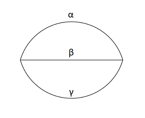
Figure 1: The two-loop sunrise graph for imaginary square masses $\alpha,\beta,\gamma$. The momenta and color charges are conserved at the vertices.

Using similar techniques, we now would like to evaluate the ($0$-leg) sunset sum-integral

$$S^{\kappa\lambda\tau}_{\alpha\beta\gamma}\equiv\int_{Q,K}G_{\alpha}(Q_{\kappa})G_{\beta}(K_{\lambda})G_{\gamma}(L_{\tau})\,,$$ (16)

where momentum and color conservation imply respectively $Q+K+L=0$ and $\kappa+\lambda+\tau=0$, see Fig. 1. We consider the case where the square masses $\alpha$, $\beta$ and $\gamma$ are purely imaginary. In fact, we restrict to those cases that are relevant for the GZ framework, where the square masses are either $0$ or $\pm im^{2}$. More precisely, it can be shown that the relevant scalar sunset sum-integrals that appear in the GZ framework are $S_{\alpha\alpha\alpha}^{\kappa\lambda\tau}$, $S_{\alpha\alpha(-\alpha)}^{\kappa\lambda\tau}$, $S_{\alpha 00}^{\kappa\lambda\tau}$, with $\smash{\alpha=\pm im^{2}}$, together of course with the corresponding permutations of masses vEgmond .

Using the spectral representation (6) in Eq. (16), we find

$$S^{\kappa\lambda\tau}_{\alpha\beta\gamma} = \int_{q_{0};{\bf q}}\rho_{\alpha}(q_{0};{\bf q})\int_{k_{0};{\bf k}}\rho_{\beta}(k_{0};{\bf k})\int_{l_{0}}\rho_{\gamma}(l_{0};{\bf l})\,{\cal S}^{\kappa\lambda\tau}(q_{0},k_{0},l_{0})\,,$$ (17)

with

$${\cal S}^{\kappa\lambda\tau}(q_{0},k_{0},l_{0}) \equiv T^{2}\sum_{n,m}\frac{1}{(q_{0}-i\omega_{n}^{\kappa})(k_{0}-i\omega_{m}^{\lambda})(l_{0}+i\omega_{m}^{\lambda}+i\omega_{n}^{\kappa})}\,,$$ (18)

a double Matsubara sum. Standard techniques for the evaluation of Matsubara sums together with color conservation $\kappa+\lambda+\tau=0$, lead then to

$${\cal S}^{\kappa\lambda\tau}(q_{0},k_{0},l_{0}) = \frac{(n_{k_{0}-i\hat{r}\cdot\lambda}-n_{l_{0}+i\hat{r}\cdot\tau})(n_{q_{0}-i\hat{r}\cdot\kappa}-n_{-l_{0}-k_{0}-i\hat{r}\cdot\kappa})}{l_{0}+k_{0}+q_{0}}$$ (19)

$$= \frac{n_{k_{0}-i\hat{r}\cdot\lambda}n_{l_{0}-i\hat{r}\cdot\tau}+(-n_{-q_{0}+i\hat{r}\cdot\kappa})n_{k_{0}-i\hat{r}\cdot\lambda}+(-n_{-q_{0}+i\hat{r}\cdot\kappa})(-n_{-l_{0}+i\hat{r}\cdot\tau})}{l_{0}+k_{0}+q_{0}}\,,$$

where, in going from the first to the second line, we have used the well known identity $n_{x}n_{y}=(1+n_{x}+n_{y})n_{x+y}$. Finally, by making use of Eq. (11), we arrive at the thermal splitting of the scalar sunset sum-integral: $S_{\alpha\beta\gamma}^{\kappa\lambda\tau}=S_{\alpha\beta\gamma}(0n)+S_{\alpha\beta\gamma}^{\kappa\lambda\tau}(1n)+S_{\alpha\beta\gamma}^{\kappa\lambda\tau}(2n)$. As in the previous example, $S_{\alpha\beta\gamma}(0n)$ denotes the pure vacuum contribution (no thermal factor), depending neither on the temperature nor on the background, while

$$S_{\alpha\beta\gamma}^{\kappa\lambda\tau}(1n)=\sum_{{\rm cyclic}}\int_{q_{0};{\bf q}}\!\!\sigma_{\alpha}^{\kappa}(q_{0};{\bf q})\,\int_{k_{0};{\bf k}}\rho_{\beta}(k_{0};{\bf k})\int_{l_{0}}\rho_{\gamma}(l_{0};{\bf l})\,\frac{\theta(l_{0})-\theta(-k_{0})}{l_{0}+k_{0}+q_{0}}\,,$$ (20)

and

$$S_{\alpha\beta\gamma}^{\kappa\lambda\tau}(2n)=\sum_{{\rm cyclic}}\int_{q_{0};{\bf q}}\sigma_{\alpha}^{\kappa}(q_{0};{\bf q})\int_{k_{0};{\bf k}}\sigma_{\beta}^{\lambda}(k_{0};{\bf k})\int_{l_{0}}\rho_{\gamma}(l_{0};{\bf l})\,\frac{1}{l_{0}+k_{0}+q_{0}}\,,$$ (21)

where $\sum_{{\rm cyclic}}$ stands for the cyclic permutations of the pairs $(\alpha,\kappa)$, $(\beta,\lambda)$ and $(\gamma,\tau)$ and $\sigma_{\alpha}^{\kappa}(q_{0};{\bf q})$ was defined in the previous section.

We note that the thermal splitting considered here assumes that the denominator $l_{0}+k_{0}+q_{0}$ never vanishes. We show in Appendix A that this is indeed so in those cases that are relevant for the GZ framework. More generic cases may require a regularization of the denominator but we shall not consider them here.

III.1 Contribution with two thermal factors

The contribution with two thermal factors is easily handled. We can first perform the $l_{0}$ integral by using the spectral representation (6) backwards. This leads to

$$S_{\alpha\beta\gamma}^{\kappa\lambda\tau}(2n)=\sum_{{\rm cyclic}}\int_{q_{0};{\bf q}}\sigma_{\alpha}^{\kappa}(q_{0};{\bf q})\int_{k_{0};{\bf k}}\sigma_{\beta}^{\lambda}(k_{0};{\bf k})\,\tilde{G}_{\gamma}(k_{0}+q_{0};{\bf l})\,,$$ (22)

where $\tilde{G}(z_{0};{\bf z})$ is defined in Eq. (6) and obeys $\tilde{G}(-z_{0};{\bf z})=\tilde{G}(z_{0};{\bf z})$. Next, we perform the $q_{0}$ and $k_{0}$ integrals and obtain

$$S_{\alpha\beta\gamma}^{\kappa\lambda\tau}(2n)=\sum_{{\rm cyclic}}\sum_{\sigma_{\alpha},\sigma_{\beta}}\int_{{\bf q}}\frac{n_{\varepsilon_{q,\alpha}-i\sigma_{\alpha}\hat{r}\cdot\kappa}}{2\varepsilon_{q,\alpha}}\int_{{\bf k}}\frac{n_{\varepsilon_{k,\beta}-i\sigma_{\beta}\hat{r}\cdot\lambda}}{2\varepsilon_{k,\beta}}\,\tilde{G}_{\gamma}(\sigma_{\alpha}\varepsilon_{q,\alpha}+\sigma_{\beta}\varepsilon_{k,\beta};{\bf l})\,,$$ (23)

where $\sigma_{\alpha}$, $\sigma_{\beta}$ and $\sigma_{\gamma}$ take values in $\{-1,+1\}$. Finally, because this contribution is UV finite, we can set $d=4$ and perform the angular integrals. We find eventually

$$S_{\alpha\beta\gamma}^{\kappa\lambda\tau}(2n)=\frac{1}{64\pi^{4}}\sum_{{\rm cyclic}}\sum_{\sigma_{\alpha},\sigma_{\beta}}\int_{0}^{\infty}dq\,q\frac{n_{\varepsilon_{q,\alpha}-i\sigma_{\alpha}\hat{r}\cdot\kappa}}{\varepsilon_{q,\alpha}}\int_{0}^{\infty}dk\,k\frac{n_{\varepsilon_{k,\beta}-i\sigma_{\beta}\hat{r}\cdot\lambda}}{\varepsilon_{k,\beta}}\ln\big{(}\alpha\beta;\gamma\big{)}\,,$$ (24)

with

$$(\alpha\beta;\gamma\big{)}\equiv\frac{-(\sigma_{\alpha}\varepsilon_{q,\alpha}+\sigma_{\beta}\varepsilon_{k,\beta})^{2}+\varepsilon_{q+k,\gamma}^{2}}{-(\sigma_{\alpha}\varepsilon_{q,\alpha}+\sigma_{\beta}\varepsilon_{k,\beta})^{2}+\varepsilon_{q-k,\gamma}^{2}}=\frac{\gamma-\alpha-\beta-2\sigma_{\alpha}\sigma_{\beta}\varepsilon_{q,\alpha}\varepsilon_{k,\beta}+2qk}{\gamma-\alpha-\beta-2\sigma_{\alpha}\sigma_{\beta}\varepsilon_{q,\alpha}\varepsilon_{k,\beta}-2qk}\,.$$ (25)

III.2 Contribution with one thermal factor

Integration over the frequencies leads this time to

$$S_{\alpha\beta\gamma}^{\kappa\lambda\tau}(1n)=\sum_{{\rm cyclic}}\sum_{\sigma_{\alpha}}\int_{\bf q}\frac{n_{\varepsilon_{q,\alpha}-i\sigma_{\alpha}\hat{r}\cdot\kappa}}{2\varepsilon_{q,\alpha}}\,\tilde{I}_{\beta\gamma}(\varepsilon_{q,\alpha};{\bf q})\,,$$ (26)

with

$$\tilde{I}_{\beta\gamma}(\varepsilon_{q,\alpha};{\bf q}) = \int_{{\bf k}}\left[\frac{1}{2\varepsilon_{l,\gamma}}\tilde{G}_{\beta}(\sigma_{\alpha}\varepsilon_{q,\alpha}+\varepsilon_{l,\gamma},{\bf k})+\frac{1}{2\varepsilon_{k,\beta}}\tilde{G}_{\beta}(\sigma_{\alpha}\varepsilon_{q,\alpha}-\varepsilon_{k,\beta},{\bf l})\right]$$ (27)

$$= \int_{{\bf k}}\frac{1}{4\varepsilon_{k,\beta}\varepsilon_{l,\gamma}}\left[\frac{1}{\varepsilon_{k,\beta}+\varepsilon_{l,\gamma}+\sigma_{\alpha}\varepsilon_{q,\alpha}}+\frac{1}{\varepsilon_{k,\beta}+\varepsilon_{l,\gamma}-\sigma_{\alpha}\varepsilon_{q,\alpha}}\right]$$

$$= \int_{{\bf k}}\frac{1}{2\varepsilon_{k,\beta}\varepsilon_{l,\gamma}}\frac{\varepsilon_{k,\beta}+\varepsilon_{l,\gamma}}{(\varepsilon_{k,\beta}+\varepsilon_{l,\gamma})^{2}-\varepsilon_{q,\alpha}^{2}}\,,$$

where we note that the dependence on $\sigma_{\alpha}$ has dropped in the last line, which explains a posteriori why we did not include it in our notation for $\tilde{I}_{\beta\gamma}(\varepsilon_{q,\alpha};{\bf q})$. We show in Appendix B that this quantity does not depend on ${\bf q}$ either. It follows that $S_{\alpha\beta\gamma}^{\kappa\lambda\tau}(1n)=\sum_{{\rm cyclic}}J_{\alpha}^{\kappa}(1n)I^{\alpha}_{\beta\gamma}(0n)$, with

$$I_{\beta\gamma}^{\alpha}(0n)\equiv\lim_{q\to 0}\tilde{I}_{\beta\gamma}(\varepsilon_{q,\alpha};{\bf q})=\int_{{\bf k}}\frac{1}{2\varepsilon_{k,\beta}\varepsilon_{k,\gamma}}\frac{\varepsilon_{k,\beta}+\varepsilon_{k,\gamma}}{(\varepsilon_{k,\beta}+\varepsilon_{k,\gamma})^{2}-\alpha}\,.$$ (28)

The case $I_{\beta\gamma}^{0}(0n)$ can be evaluated immediately as

$$I^{0}_{\beta\gamma}(0n) = \int_{k}\frac{1}{2\varepsilon_{k,\beta}\varepsilon_{k,\gamma}}\frac{1}{\varepsilon_{k,\beta}+\varepsilon_{k,\gamma}}$$ (29)

$$= \int_{k}\frac{1}{2\varepsilon_{k,\beta}\varepsilon_{k,\gamma}}\frac{\varepsilon_{k,\beta}-\varepsilon_{k,\gamma}}{\beta-\gamma}=-\frac{J_{\beta}(0n)-J_{\gamma}(0n)}{\beta-\gamma}\,.$$

As for the general case $I_{\beta\gamma}^{\alpha}(0n)$, we show in Appendix B that it can be obtained from the analytic continuation of the vacuum Euclidean integral

$$I_{\beta\gamma}(0n)(Q^{2}\geq 0)\equiv\int_{K}^{T=0}G_{\beta}(K)G_{\gamma}(L)\,.$$ (30)

We find

$$I_{\beta\gamma}^{\alpha}(0n)=\frac{1}{16\pi^{2}}\left\{\frac{1}{\epsilon}-\ln\frac{\bar{\mu}^{2}}{\alpha}+2\right.$$

$$\hskip 91.04872pt+\,\frac{R(\alpha^{-},\beta,\gamma)-\alpha-\beta+\gamma}{2\alpha}\ln\frac{R(\alpha^{-},\beta,\gamma)-\alpha-\beta+\gamma}{2\bar{\mu}^{2}}$$

$$\hskip 91.04872pt-\,\frac{R(\alpha^{-},\beta,\gamma)+\alpha-\beta+\gamma}{2\alpha}\ln\frac{R(\alpha^{-},\beta,\gamma)+\alpha-\beta+\gamma}{2\bar{\mu}^{2}}$$

$$\hskip 91.04872pt-\,\frac{R(\alpha^{-},\beta,\gamma)+\alpha+\beta-\gamma}{2\alpha}\ln\frac{R(\alpha^{-},\beta,\gamma)+\alpha+\beta-\gamma}{2\bar{\mu}^{2}}$$

$$\hskip 91.04872pt\left.+\,\frac{R(\alpha^{-},\beta,\gamma)-\alpha+\beta-\gamma}{2\alpha}\ln\frac{R(\alpha^{-},\beta,\gamma)-\alpha+\beta-\gamma}{2\bar{\mu}^{2}}\right\}\!,$$ (31)

with $\alpha^{-}\equiv\alpha-0^{+}$ and

$$R^{2}(\alpha,\beta,\gamma)\equiv\alpha^{2}+\beta^{2}+\gamma^{2}-2\alpha\beta-2\beta\gamma-2\gamma\alpha\,.$$ (32)

More details on the continuation are given in Appendix B.

III.3 Vacuum contribution (no thermal factor)

The vacuum contribution can be written as a standard $d$-dimensional Euclidean integral

$$S_{\alpha\beta\gamma}(0n)\equiv\int_{Q,K}^{T=0}G_{\alpha}(Q)G_{\beta}(K)G_{\gamma}(L)\,.$$ (33)

This integral is known analytically for positive square masses $\alpha$, $\beta$ and $\gamma$ Caffo:1998du . One strategy to obtain the corresponding integral for imaginary square masses is to perform an analytic continuation of the result of Caffo:1998du with respect to the masses. This is an efficient strategy in the case where the non-vanishing masses are all equal.

Let us take for instance $S_{\alpha 00}(0n)$. Seen as function of a complex $\alpha$, it is analytic with a branch cut for $\alpha\in\rm Re^{-}$. Because the expression for $\alpha\in\rm Re^{+}$,

$$S_{\alpha 00}(0n) = (4\pi\mu^{2})^{2\epsilon}\Gamma\left(1+\epsilon\right)^{2}\left(-\frac{\alpha}{128\pi^{4}}\right)\Bigg{[}\frac{1}{4\epsilon^{2}}-\frac{1}{2\epsilon}\left(\ln\alpha-\frac{3}{2}\right)$$ (34)

$$\hskip 142.26378pt+\,\frac{1}{2}\Bigg{(}\!\ln^{2}(\alpha)-3\ln(\alpha)+\frac{\pi^{2}}{6}+\frac{7}{2}\Bigg{)}\Bigg{]},$$

has branch cuts only for $\alpha\in\rm Re^{-}$, it can be immediately used to represent $S_{\alpha 00}(0n)$ in the case where $\alpha$ is purely imaginary. Using a similar argument, we obtain

$$S_{\alpha\alpha\alpha}(0n) = (4\pi\mu^{2})^{2\epsilon}\Gamma\left(1+\epsilon\right)^{2}\left(-\frac{\alpha}{128\pi^{4}}\right)\Bigg{[}\frac{3}{4\epsilon^{2}}-\frac{1}{2\epsilon}\left(3\ln\alpha-\frac{9}{2}\right)$$ (35)

$$+ \left(\frac{3}{2}\ln^{2}\left(\alpha\right)-\frac{9}{2}\ln\left(\alpha\right)-i\sqrt{3}\text{Li}_{2}\left(\frac{1}{2}-\frac{i\sqrt{3}}{2}\right)+\frac{i\pi^{2}}{12\sqrt{3}}+\frac{21}{4}\right)\Bigg{]}.$$

The evaluation of $S_{\alpha\alpha(-\alpha)}(0n)$ is trickier because it involves the analytic continuation of a function of two complex variables. Although this can be done in principle, we here chose a more direct evaluation by adapting the technique in Ref. Caffo:1998du to the case of imaginary square masses. This technique is based on the derivation of a differential equation satisfied by $S_{\alpha\beta\gamma}(0n)$. Although the derivation of the differential equation is not affected by the presence of imaginary square masses, we reproduce it here for completeness and because we shall use it for other purposes later.

Let us write the scalar sunset vacuum integral symbolically as

$$\left\{G_{\alpha}G_{\beta}G_{\gamma}\right\}\equiv\int_{Q,K}^{T=0}G_{\alpha}(Q)G_{\beta}(K)G_{\gamma}(L)\,,$$ (36)

with $L=-Q-K$. Expanding the identities

$$0=\left\{-\frac{\partial}{\partial Q_{\mu}}\Big{(}K_{\mu}\,G_{\alpha}G_{\beta}G_{\gamma}\Big{)}\right\}=\left\{-\frac{\partial}{\partial Q_{\mu}}\Big{(}Q_{\mu}\,G_{\alpha}G_{\beta}G_{\gamma}\Big{)}\right\}\!,$$ (37)

we find

$$0 = \left\{2Q\cdot K\,G^{2}_{\alpha}G_{\beta}G_{\gamma}\right\}-\left\{2L\cdot K\,G_{\alpha}G_{\beta}G^{2}_{\gamma}\right\},$$ (38)

$$0 = -d\left\{G_{\alpha}G_{\beta}G_{\gamma}\right\}+\left\{2Q^{2}\,G^{2}_{\alpha}G_{\beta}G_{\gamma}\right\}-\left\{2Q\cdot L\,G_{\alpha}G_{\beta}G^{2}_{\gamma}\right\}.$$ (39)

Then, writing $Q^{2}=Q^{2}+\alpha-\alpha$, as well as

$$2Q\cdot K = L^{2}+\gamma-Q^{2}-\alpha-K^{2}-\beta+(\alpha+\beta-\gamma)\,,$$ (40)

$$2L\cdot K = Q^{2}+\alpha-K^{2}-\beta-L^{2}-\gamma+(\beta+\gamma-\alpha)\,,$$ (41)

$$2Q\cdot L = K^{2}+\beta-L^{2}-\gamma-Q^{2}-\alpha+(\gamma+\alpha-\beta)\,,$$ (42)

we arrive at

$$0 = \left\{G^{2}_{\alpha}G_{\beta}\right\}-\left\{G^{2}_{\alpha}G_{\gamma}\right\}+(\alpha+\beta-\gamma)\left\{G^{2}_{\alpha}G_{\beta}G_{\gamma}\right\}$$ (43)

$$- \left\{G_{\beta}G^{2}_{\gamma}\right\}+\left\{G_{\alpha}G^{2}_{\gamma}\right\}-(\beta+\gamma-\alpha)\left\{G_{\alpha}G_{\beta}G^{2}_{\gamma}\right\},$$

$$0 = (3-d)\left\{G_{\alpha}G_{\beta}G_{\gamma}\right\}-2\alpha\left\{G^{2}_{\alpha}G_{\beta}G_{\gamma}\right\}$$ (44)

$$- \left\{G_{\alpha}G^{2}_{\gamma}\right\}+\left\{G_{\beta}G^{2}_{\gamma}\right\}-(\gamma+\alpha-\beta)\left\{G_{\alpha}G_{\beta}G^{2}_{\gamma}\right\}.$$

Using the first relation in order to replace $\{G^{2}_{\alpha}G_{\beta}G_{\gamma}\}$ in the second, we find

$$0 = (3-d)(\alpha+\beta-\gamma)\left\{G_{\alpha}G_{\beta}G_{\gamma}\right\}+R^{2}(\alpha,\beta,\gamma)\left\{G_{\alpha}G_{\beta}G^{2}_{\gamma}\right\}$$ (45)

$$+ (\alpha-\beta+\gamma)(\left\{G_{\alpha}G^{2}_{\gamma}\right\}-\left\{G_{\beta}G^{2}_{\gamma}\right\})+2\alpha(\left\{G^{2}_{\alpha}G_{\beta}\right\}-\left\{G^{2}_{\alpha}G_{\gamma}\right\})\,.$$

Finally, using that $\{G_{\alpha}^{2}G_{\beta}\}=\{G_{\alpha}^{2}\}\{G_{\beta}\}$, this rewrites

$$R^{2}(\alpha,\beta,\gamma)S_{\alpha\beta\gamma^{2}}(0n) \,=\, (d-3)(\alpha+\beta-\gamma)S_{\alpha\beta\gamma}(0n)+(d-2)J_{\alpha}(0n)J_{\beta}(0n)$$ (46)

$$- (\alpha-\beta-\gamma)J_{\alpha}(0n)J_{\gamma^{2}}(0n)-(\beta-\alpha-\gamma)J_{\beta}(0n)J_{\gamma^{2}}(0n)\,,$$

where we have introduced the notations $J_{\alpha^{2}}(0n)\equiv\{G_{\alpha}^{2}\}$ and $S_{\alpha\beta\gamma^{2}}(0n)\equiv\left\{G_{\alpha}G_{\beta}G_{\gamma^{2}}\right\}$. In the case where $\gamma\neq 0$, we can use

$$J_{\gamma^{2}}(0n) = -\frac{\partial}{\partial\gamma}J_{\gamma}(0n)=(1-d/2)\frac{J_{\gamma}(0n)}{\gamma}\,,$$ (47)

$$S_{\alpha\beta\gamma^{2}}(0n) = -\frac{\partial}{\partial\gamma}S_{\alpha\beta\gamma}(0n)\,,$$ (48)

to arrive at the differential equation

$$R^{2}(\alpha,\beta,\gamma)\frac{\partial}{\partial\gamma}S_{\alpha\beta\gamma}(0n) \,=\, (3-d)(\alpha+\beta-\gamma)S_{\alpha\beta\gamma}(0n)+(2-d)J_{\alpha}(0n)J_{\beta}(0n)$$

$$+ (2-d)\left[\frac{\alpha-\beta-\gamma}{2\gamma}J_{\alpha}(0n)J_{\gamma}(0n)+\frac{\beta-\alpha-\gamma}{2\gamma}J_{\beta}(0n)J_{\gamma}(0n)\right]\!.$$

In Appendix C, we use this equation to obtain $S_{\alpha\alpha\gamma}(0n)$ in some appropriate range of values for $\gamma$. We follow the approach of Ref. Caffo:1998du by carefully adapting it to the case of imaginary square masses. We find in particular

$$S_{\alpha\alpha(-\alpha)}(0n)$$

$$\hskip 14.22636pt=\,(4\pi\mu^{2})^{2\epsilon}\Gamma\left(1+\epsilon\right)^{2}\left(-\frac{\alpha}{128\pi^{4}}\right)\Bigg{[}\frac{1}{4\epsilon^{2}}+\frac{1}{2\epsilon}\left(\frac{3}{2}-2\ln\alpha+\ln(-\alpha)\right)$$

$$\hskip 71.13188pt+\,\frac{\sqrt{5}}{2}\left(\frac{\pi^{2}}{5}-i\pi\ln\frac{3-\sqrt{5}}{2}\right)$$

$$\hskip 71.13188pt+\,\frac{7}{4}-3\ln\alpha+\frac{3}{2}\ln(-\alpha)-\frac{1}{2}\ln\alpha\ln(-\alpha)+\frac{5}{4}\ln^{2}\alpha-\frac{1}{4}\ln^{2}(-\alpha)\Bigg{]}.$$ (50)

We mention that the vacuum integrals $S_{+++}(0n)$, $S_{+00}(0n)$ and $S_{++-}(0n)$ have also been used in Gracey:2005cx ; Gracey:2010cg but the individual results are not quoted, only their final combination in the vacuum GZ horizon condition at two-loop order. For similar integrals involving both real and imaginary square masses, see Ford:2009ar .

III.4 Summary

In summary, the scalar sunset sum-integral can be split as

$$S_{\alpha\beta\gamma}^{\kappa\lambda\tau} = S_{\alpha\beta\gamma}(0n)+S_{\alpha\beta\gamma}^{\kappa\lambda\tau}(1n)+S_{\alpha\beta\gamma}^{\kappa\lambda\tau}(2n)\,,$$ (51)

with $S_{\alpha\beta\gamma}(0n)$ given in Eqs. (34), (35) or (50) depending on the considered case, while $S_{\alpha\beta\gamma}^{\kappa\lambda\tau}(1n)$ reads

$$S_{\alpha\beta\gamma}^{\kappa\lambda\tau}(1n)=J_{\alpha}^{\kappa}(1n)I^{\alpha}_{\beta\gamma}(0n)+J_{\beta}^{\lambda}(1n)I^{\beta}_{\gamma\alpha}(0n)+J_{\gamma}^{\tau}(1n)I^{\gamma}_{\alpha\beta}(0n)\,,$$ (52)

with $I_{\beta\gamma}^{\alpha}(0n)$ given in Eq. (III.2), and $S_{\alpha\beta\gamma}^{\kappa\lambda\tau}(2n)$ is given in Eq. (24).

IV Mass derivatives

The various sunset diagrams that appear in the GZ framework lead also to mass derivatives of the scalar sunset, in the limit where the corresponding mass is taken to zero. In fact, what appear are the limits vEgmond

$$\Delta S^{\kappa\lambda\tau}_{0^{2}\beta\gamma} \equiv \lim_{\alpha\to 0}\left[S^{\kappa\lambda\tau}_{\alpha^{2}\beta\gamma}+J_{\alpha^{2}}^{\kappa}\frac{J_{\beta}^{\lambda}-J_{\gamma}^{\tau}}{\beta-\gamma}\right]\!,$$ (53)

$$\Delta S^{\kappa\lambda\tau}_{0^{2}0^{2}\gamma} \equiv \lim_{\alpha\to 0}\lim_{\beta\to 0}\left[S^{\kappa\lambda\tau}_{\alpha^{2}\beta^{2}\gamma}-\frac{J_{\alpha^{2}}^{\kappa}J_{\beta^{2}}^{\lambda}}{\gamma}-\frac{J_{\gamma}^{\tau}-J_{0}^{\kappa}}{\gamma^{2}}J_{\beta^{2}}^{\lambda}-\frac{J_{\gamma}^{\tau}-J_{0}^{\lambda}}{\gamma^{2}}J_{\alpha^{2}}^{\kappa}\right]\!,$$ (54)

where, as already introduced above, the squaring of the mass indices corresponds to the doubling of the associated propagators, or more generally to taking minus the derivative with respect to the associated square mass. The relevant cases for the GZ framework are $\Delta S^{\kappa\lambda\tau}_{0^{2}\gamma(-\gamma)}$, $\Delta S^{\kappa\lambda\tau}_{0^{2}0\gamma}$, $\Delta S^{\kappa\lambda\tau}_{0^{2}0^{2}\gamma}$, with $\smash{\gamma=\pm im^{2}}$, together with the corresponding permutations of the masses vEgmond . We also mention that $\Delta S_{0^{2},\alpha\beta}$ is nothing but the function $\bar{T}$ defined in Martin:2003qz , for zero external momentum but generalized to the case of finite temperature.

It is easily seen that, even though $S^{\kappa\lambda\tau}_{\alpha^{2}\beta\gamma}$, $S^{\kappa\lambda\tau}_{\alpha^{2}\beta^{2}\gamma}$, $J_{\alpha^{2}}^{\kappa}$ and $J_{\beta^{2}}^{\lambda}$ are singular in the limits $\alpha\to 0$ or $\beta\to 0$, the combinations of sum-integrals in Eqs. (53) and (54) admit regular limits. To verify this, let us first note that the potential singularities originate either from the vacuum pieces which do not depend on the color weights ($\kappa$, $\lambda$, $\tau$), or from the thermal pieces in the case where the weights are equal to zero. Therefore, one can safely ignore the weights in order to check the regularity of the above limits. For instance, in the limit $\alpha\to 0$, the sum-integral $S_{\alpha^{2}\beta\gamma}$ is dominated by the $Q\to 0$ region and behaves consequently as

$$S_{\alpha^{2}\beta\gamma}\sim\int_{Q}\frac{1}{(Q^{2}+\alpha)^{2}}\times\int_{K}\frac{1}{(K^{2}+\beta)(K^{2}+\gamma)}=-J_{\alpha^{2}}\frac{J_{\beta}-J_{\gamma}}{\beta-\gamma}\,.$$ (55)

The divergent behavior in the RHS is precisely what is subtracted in Eq. (53) to ensure that the limit is regular. To understand the singular structure of $S_{\alpha^{2}\beta^{2}\gamma}$, we first write it identically as

$$S_{\alpha^{2}\beta^{2}\gamma} = \frac{1}{\gamma}\int_{Q,K}\frac{1}{(Q^{2}+\alpha)^{2}}\frac{1}{(K^{2}+\beta)^{2}}$$ (56)

$$- \frac{1}{\gamma}\int_{Q,K}\frac{1}{(Q^{2}+\alpha)^{2}}\frac{1}{(K^{2}+\beta)^{2}}\frac{K^{2}+Q^{2}+2K\cdot Q}{(K+Q)^{2}+\gamma}\,.$$

The term with $K\cdot Q$ in the second line leads to regular contributions in the limit $\alpha\to 0$ and $\beta\to 0$, while the term with $K^{2}$ (resp. $Q^{2}$) leads to singular contributions as $\alpha\to 0$ (resp. $\beta\to 0$), controlled by the $Q\to 0$ (resp. $K\to 0$) region of the integral. We find

$$S_{\alpha^{2}\beta^{2}\gamma} = \frac{1}{\gamma}\int_{Q}\frac{1}{(Q^{2}+\alpha)^{2}}\int_{K}\frac{1}{(K^{2}+\beta)^{2}}$$ (57)

$$- \frac{1}{\gamma}\int_{Q}\frac{1}{(Q^{2}+\alpha)^{2}}\int_{K}\frac{1}{K^{2}(K^{2}+\gamma)}$$

$$- \frac{1}{\gamma}\int_{Q}\frac{1}{Q^{2}(Q^{2}+\alpha)}\int_{K}\frac{1}{(K^{2}+\beta)^{2}}+{\rm regular}$$

$$= \frac{J_{\alpha^{2}}J_{\beta^{2}}}{\gamma}+\frac{J_{\gamma}-J_{0}}{\gamma^{2}}J_{\alpha^{2}}+\frac{J_{\gamma}-J_{0}}{\gamma^{2}}J_{\beta^{2}}+{\rm regular}\,.$$

These are precisely the terms that are subtracted in Eq. (54) to obtain a regular limit.

The regular limits $\Delta S^{\kappa\lambda\tau}_{0^{2}\beta\gamma}$ and $\Delta S^{\kappa\lambda\tau}_{0^{2}0^{2}\gamma}$ admit thermal splittings that one derives from the corresponding splitting (51) of the scalar sunset, and which we now discuss.

IV.1 Thermal splitting

From Eqs. (51) and (53), we find the thermal splitting

$$\Delta S^{\kappa\lambda\tau}_{0^{2}\beta\gamma}=\Delta S_{0^{2}\beta\gamma}(0n)+\Delta S^{\kappa\lambda\tau}_{0^{2}\beta\gamma}(1n)+\Delta S^{\kappa\lambda\tau}_{0^{2}\beta\gamma}(2n)\,,$$ (58)

with

$$\Delta S_{0^{2}\beta\gamma}(0n) \!=\! \lim_{\alpha\to 0}\!\left[S_{\alpha^{2}\beta\gamma}(0n)\!+\!J_{\alpha^{2}}(0n)\frac{J_{\beta}(0n)-J_{\gamma}(0n)}{\beta-\gamma}\right]\!,$$ (59)

$$\Delta S^{\kappa\lambda\tau}_{0^{2}\beta\gamma}(1n) \!=\! \lim_{\alpha\to 0}\!\left[S^{\kappa\lambda\tau}_{\alpha^{2}\beta\gamma}(1n)\!+\!J_{\alpha^{2}}(0n)\frac{J_{\beta}^{\lambda}(1n)-J_{\gamma}^{\tau}(1n)}{\beta-\gamma}\!+\!J_{\alpha^{2}}^{\kappa}(1n)\frac{J_{\beta}(0n)-J_{\gamma}(0n)}{\beta-\gamma}\right]\!,$$ (60)

$$\Delta S^{\kappa\lambda\tau}_{0^{2}\beta\gamma}(2n) \!=\! \lim_{\alpha\to 0}\!\left[S^{\kappa\lambda\tau}_{\alpha^{2}\beta\gamma}(2n)\!+\!J_{\alpha^{2}}^{\kappa}(1n)\frac{J_{\beta}^{\lambda}(1n)-J_{\gamma}^{\tau}(1n)}{\beta-\gamma}\right]\!.$$ (61)

Similarly, from Eqs. (51) and (54), we find the thermal splitting

$$\Delta S^{\kappa\lambda\tau}_{0^{2}0^{2}\gamma}=\Delta S_{0^{2}0^{2}\gamma}(0n)+\Delta S^{\kappa\lambda\tau}_{0^{2}0^{2}\gamma}(1n)+\Delta S^{\kappa\lambda\tau}_{0^{2}0^{2}\gamma}(2n)\,,$$ (62)

with

$$\Delta S_{0^{2}0^{2}\gamma}(0n) \!=\! \lim_{\alpha\to 0}\lim_{\beta\to 0}\left[S_{\alpha^{2}\beta^{2}\gamma}(0n)-\frac{J_{\alpha^{2}}(0n)J_{\beta^{2}}(0n)}{\gamma}-\frac{J_{\alpha^{2}}(0n)+J_{\beta^{2}}(0n)}{\gamma^{2}}J_{\gamma}(0n)\right]\!,$$ (63)

$$\Delta S^{\kappa\lambda\tau}_{0^{2}0^{2}\gamma}(1n) \!=\! \lim_{\alpha\to 0}\lim_{\beta\to 0}\left[S^{\kappa\lambda\tau}_{\alpha^{2}\beta^{2}\gamma}(1n)-\frac{J_{\alpha^{2}}(0n)J_{\beta^{2}}^{\lambda}(1n)}{\gamma}-\frac{J_{\alpha^{2}}^{\kappa}(1n)J_{\beta^{2}}(0n)}{\gamma}\right.$$ (64)

$$\hskip 102.43008pt-\,\frac{J_{\gamma}(0n)}{\gamma^{2}}J_{\beta^{2}}^{\lambda}(1n)-\frac{J_{\gamma}^{\tau}(1n)-J_{0}^{\kappa}(1n)}{\gamma^{2}}J_{\beta^{2}}(0n)$$

$$\hskip 102.43008pt\left.-\,\frac{J_{\gamma}(0n)}{\gamma^{2}}J_{\alpha^{2}}^{\kappa}(1n)-\frac{J_{\gamma}^{\tau}(1n)-J_{0}^{\lambda}(1n)}{\gamma^{2}}J_{\alpha^{2}}(0n)\right]\!,$$

$$\Delta S^{\kappa\lambda\tau}_{0^{2}0^{2}\gamma}(2n) \!=\! \lim_{\alpha\to 0}\lim_{\beta\to 0}\left[S^{\kappa\lambda\tau}_{\alpha^{2}\beta^{2}\gamma}(2n)-\frac{J_{\alpha^{2}}^{\kappa}(1n)J_{\beta^{2}}^{\lambda}(1n)}{\gamma}\right.$$ (65)

$$\hskip 48.36958pt\left.-\,\frac{J_{\gamma}^{\tau}(1n)-J_{0}^{\kappa}(1n)}{\gamma^{2}}J_{\beta^{2}}^{\lambda}(1n)-\frac{J_{\gamma}^{\tau}(1n)-J_{0}^{\lambda}(1n)}{\gamma^{2}}J_{\alpha^{2}}^{\kappa}(1n)\right]\!,$$

where we have used that $\smash{J_{0}(0n)=0}$. In what follows, we shall also make extensive use of the property $\smash{J_{0^{2}}(0n)=0}$, valid in dimensional regularization . This property might be more difficult to grasp than the previous one because $J_{\alpha^{2}}(0n)$ diverges in the limit $\smash{\alpha\to 0}$. However this just means that the function $J_{\alpha^{2}}(0n)$, although defined for $\smash{\alpha=0}$, is not continuous at $\smash{\alpha=0}$. Then, we shall always make sure that when the property $\smash{J_{0^{2}}(0n)=0}$ is used, it corresponds to $J_{\alpha^{2}}(0n)$ being evaluated for $\smash{\alpha=0}$ and not to a limit being taken. We mention finally that the results to be presented below can be obtained without ever using $\smash{J_{0^{2}}(0n)=0}$ although the calculations are lengthier.

IV.2 Vacuum contributions (no thermal factor)

$\Delta S_{0^{2}\beta\gamma}(0n)$: The vacuum contribution $\Delta S_{0^{2}\beta\gamma}(0n)$ is in fact nothing but $S_{0^{2}\beta\gamma}(0n)$. Indeed, even though both $S_{\alpha^{2}\beta\gamma}(0n)$ and $J_{\alpha^{2}}(0n)$ are singular in the limit $\smash{\alpha\to 0}$, their particular combination in Eq. (59) is regular. Moreover since $S_{0^{2}\beta\gamma}(0n)$ and $J_{0^{2}}(0n)$ are well defined in dimensional regularization, the limit $\smash{\gamma\to 0}$ is then equivalent to the direct evaluation at $\smash{\gamma=0}$, and we find $\smash{\Delta S_{0^{2}\beta\gamma}(0n)=S_{0^{2}\beta\gamma}(0n)}$ owing to the fact that $\smash{J_{0^{2}}(0n)=0}$. Now, since Eq. (46) is valid for $\smash{\gamma=0}$, and using once more the property $\smash{J_{0^{2}}(0n)=0}$, we arrive at

$$S_{0^{2}\beta\gamma}(0n)=(d-3)\frac{\beta+\gamma}{(\beta-\gamma)^{2}}S_{0\beta\gamma}(0n)+(d-2)\frac{J_{\beta}(0n)J_{\gamma}(0n)}{(\beta-\gamma)^{2}}\,,$$ (66)

which expresses $\Delta S_{\alpha\beta 0^{2}}(0n)$ in terms of already determined functions. We notice that, in the case of $\Delta S_{0^{2}\gamma(-\gamma)}$, the term proportional to $S_{0\gamma(-\gamma)}(0n)$ vanishes and therefore we do not need to consider this vacuum sunset integral.

$\Delta S_{0^{2}0^{2}\gamma}(0n)$: We can proceed similarly for $\Delta S_{0^{2}0^{2}\gamma}(0n)$. First, from the same argument as above, we find $\smash{\Delta S_{0^{2}0^{2}\gamma}(0n)=S_{0^{2}0^{2}\gamma}(0n)}$. The difference with the above is that we do not have an equation fixing directly $S_{0^{2}0^{2}\gamma}(0n)$. Acting on Eq. (66) with $-\partial/\partial\beta$, we obtain an equation for $S_{0^{2}\beta^{2}\gamma}(0n)$ with $\smash{\beta\neq 0}$, but $S_{0^{2}0^{2}\gamma}(0n)$ is not the limit of $S_{0^{2}\beta^{2}\gamma}(0n)$. The way out is to subtract from $S_{0^{2}\beta^{2}\gamma}$ its $\smash{\beta\to 0}$ divergent part, in such a way that

$$S_{0^{2}0^{2}\gamma}(0n)=\lim_{\beta\to 0}\left[S_{0^{2}\beta^{2}\gamma}(0n)-\frac{J_{\beta^{2}}(0n)J_{\gamma}(0n)}{\gamma^{2}}\right],$$ (67)

owing again to $\smash{J_{0^{2}}(0n)=0}$. We find

$$S_{0^{2}\beta^{2}\gamma}(0n)-\frac{J_{\beta^{2}}(0n)J_{\gamma}(0n)}{\gamma^{2}}$$

$$\hskip 14.22636pt=\,(d-3)\frac{\beta+3\gamma}{(\beta-\gamma)^{3}}S_{0\beta\gamma}(0n)+(d-3)\frac{\beta+\gamma}{(\beta-\gamma)^{2}}\left[S_{0\beta^{2}\gamma}(0n)+\frac{J_{\beta^{2}}(0n)J_{\gamma}(0n)}{\gamma}\right]$$

$$\hskip 14.22636pt+\,2(d-2)\frac{J_{\beta}(0n)J_{\gamma}(0n)}{(\beta-\gamma)^{3}}+\left[\frac{d-2}{(\beta-\gamma)^{2}}-\frac{1}{\gamma^{2}}-\frac{d-3}{(\beta-\gamma)^{2}}\frac{\beta+\gamma}{\gamma}\right]J_{\beta^{2}}(0n)J_{\gamma}(0n)\,.$$ (68)

The dangerous contributions proportional to $J_{\beta^{2}}(0n)$ in the RHS cancel in the limit $\smash{\beta\to 0}$ and we find eventually

$$S_{0^{2}0^{2}\gamma}(0n) = -3(d-3)\frac{S_{00\gamma}(0n)}{\gamma^{2}}+(d-3)\frac{S_{00^{2}\gamma}(0n)}{\gamma}\,,$$ (69)

$$= (d-3)(d-6)\frac{S_{00\gamma}(0n)}{\gamma^{2}}\,,$$

where we have once more made use of Eq. (66). We have cross-checked this last result using a direct evaluation of $S_{0^{2}0^{2}\gamma}(0n)$ using standard techniques.

IV.3 Contributions with one thermal factor

$\Delta S^{\kappa\lambda\tau}_{0^{2}\beta\gamma}(1n)$: The contribution with one thermal factor to $\Delta S^{\kappa\lambda\tau}_{0^{2}\beta\gamma}$ can be rewritten as

$$\Delta S^{\kappa\lambda\tau}_{0^{2}\beta\gamma}(1n) \!=\! \lim_{\alpha\to 0}\Bigg{[}J_{\alpha^{2}}^{\kappa}(1n)I^{\alpha}_{\beta\gamma}(0n)+J_{\alpha}^{\kappa}(1n)I^{\alpha^{2}}_{\beta\gamma}(0n)+J_{\beta}^{\lambda}(1n)I^{\beta}_{\alpha^{2}\gamma}(0n)+J_{\gamma}^{\tau}(1n)I^{\gamma}_{\alpha^{2}\beta}(0n)$$ (70)

$$\hskip 22.76228pt+\,J_{\alpha^{2}}(0n)\frac{J_{\beta}^{\lambda}(1n)-J_{\gamma}^{\tau}(1n)}{\beta-\gamma}+J_{\alpha^{2}}^{\kappa}(1n)\frac{J_{\beta}(0n)-J_{\gamma}(0n)}{\beta-\gamma}\Bigg{]}$$

$$\!=\! \lim_{\alpha\to 0}\Bigg{[}J_{\alpha^{2}}^{\kappa}(1n)\left(I^{\alpha}_{\beta\gamma}(0n)+\frac{J_{\beta}(0n)-J_{\gamma}(0n)}{\beta-\gamma}\right)+J_{\alpha}^{\kappa}(1n)I^{\alpha^{2}}_{\beta\gamma}(0n)$$

$$\hskip 22.76228pt+\,J_{\beta}^{\lambda}(1n)\left(I^{\beta}_{\alpha^{2}\gamma}(0n)+\frac{J_{\alpha^{2}}(0n)}{\beta-\gamma}\right)\!+\!J_{\gamma}^{\tau}(1n)\left(I^{\gamma}_{\alpha^{2}\beta}(0n)+\frac{J_{\alpha^{2}}(0n)}{\gamma-\beta}\right)\Bigg{]}.$$

Owing to Eq. (29), it seems that the contribution in the first round bracket can be neglected in the limit $\smash{\alpha\to 0}$. This turns out to be true, although one needs to pay a little bit of attention, since, at finite temperature and in the case where $\smash{\kappa=0}$, $J_{\alpha^{2}}^{\kappa}(1n)$ diverges in the same limit. Fortunately, the divergence goes as $\alpha^{-1/2}$, which is not enough to compensate the vanishing of the round bracket $\sim\alpha$. We find eventually that

$$\Delta S^{\kappa\lambda\tau}_{0^{2}\beta\gamma}(1n)=J_{0}^{\kappa}(1n)\Delta I^{0^{2}}_{\beta\gamma}(0n)+J_{\beta}^{\lambda}(1n)\Delta I^{\beta}_{0^{2}\gamma}(0n)+J_{\gamma}^{\tau}(1n)\Delta I^{\gamma}_{0^{2}\beta}(0n)\,,$$ (71)

with

$$\Delta I^{0^{2}}_{\beta\gamma}(0n) \equiv I^{0^{2}}_{\beta\gamma}(0n)\,,$$ (72)

$$\Delta I^{\beta}_{0^{2}\gamma}(0n) \equiv \lim_{\alpha\to 0}\left[I^{\beta}_{\alpha^{2}\gamma}(0n)+\frac{J_{\alpha^{2}}(0n)}{\beta-\gamma}\right]=I^{\beta}_{0^{2}\gamma}(0n)\,,$$ (73)

where the contribution within brackets is regular in the limit $\smash{\alpha\to 0}$ and we have used $\smash{J_{0^{2}}(0n)=0}$ in the last step.

The first quantity can be computed using similar tricks as for $I_{\beta\gamma}^{0}(0n)$ in the previous section, namely

$$\Delta I^{0^{2}}_{\beta\gamma}(0n) = -\int_{k}\frac{1}{2\varepsilon_{k,\beta}\varepsilon_{k,\gamma}}\frac{1}{(\varepsilon_{k,\beta}+\varepsilon_{k,\gamma})^{3}}=-\int_{k}\frac{1}{2\varepsilon_{k,\beta}\varepsilon_{k,\gamma}}\frac{(\varepsilon_{k,\beta}-\varepsilon_{k,\gamma})^{3}}{(\beta-\gamma)^{3}}$$ (74)

$$= -\int_{k}\frac{(\varepsilon^{2}_{k,\beta}+3\varepsilon^{2}_{k,\gamma})/\varepsilon_{k,\gamma}-(\varepsilon^{2}_{k,\gamma}+3\varepsilon^{2}_{k,\beta})/\varepsilon_{k,\beta}}{2(\beta-\gamma)^{3}}$$

$$= \frac{1}{(\gamma-\beta)^{3}}\left[\left(\beta+\frac{4-d}{d}\gamma\right)J_{\gamma}(0n)-\left(\gamma+\frac{4-d}{d}\beta\right)J_{\beta}(0n)\right],$$

where we have used that

$$\int_{k}\frac{k^{2}}{2\varepsilon_{k,\beta}}=\int_{K}^{T=0}\frac{k^{2}}{K^{2}+\beta}=-\frac{d-1}{d}\beta J_{\beta}(0n)\,,$$ (75)

together with $\int_{K}^{T=0}1=0$ in dimensional regularization.

As for $\Delta I^{\beta}_{0^{2}\gamma}(0n)$, we can proceed in many different ways, either by acting with $-\partial/\partial\alpha$ on the previously determined expression for $I_{\alpha\gamma}^{\beta}(0n)$, followed by the $\alpha\to 0$ limit after appropriate subtraction of the $\smash{\alpha\to 0}$ singular part, or by computing the appropriate subtracted Euclidean integral

$$\Delta I_{0^{2}\gamma}(0n)(K^{2})\equiv\lim_{\alpha\to 0}\left[I_{\alpha^{2}\gamma}(K^{2})-\frac{J_{\alpha^{2}}(0n)}{K^{2}+\gamma}\right]=I_{0^{2}\gamma}(K^{2})\,,$$ (76)

and analytically continuing it from $K^{2}>0$ to $K^{2}=-\beta$ imaginary. Here we proceed with this second strategy but instead of continuing the explicit expression of the integral, we continue the corresponding differential equation, with the advantage that $\Delta I^{\beta}_{0^{2}\gamma}(0n)$ will be expressed in terms of already computed quantities.

To derive the differential equation, we basically consider the same equations as in Eqs. (37) but with the propagator $G_{\beta}(K)$ and the integral $\int_{K}^{T=0}$ missing. It is easily seen that one can follow the steps below Eqs. (37) by removing the factors $G_{\beta}(K)$ (those terms that did not have such a factor need to be discarded) and to replace the explicit occurrences of $\beta$ by $-K^{2}$. It follows that

$$R^{2}(\gamma,-K^{2},\alpha)I_{\alpha^{2}\gamma}(0n)(K^{2}) = (d-3)(\gamma-K^{2}-\alpha)I_{\alpha\gamma}(0n)(K^{2})$$ (77)

$$+ (d-2)J_{\gamma}(0n)+(K^{2}+\alpha+\gamma)J_{\alpha^{2}}(0n)\,.$$

This identity is valid for $\smash{\alpha=0}$, in which case, we obtain

$$I_{0^{2}\gamma}(0n)(K^{2})=\frac{(d-3)(\gamma-K^{2})I_{0\gamma}(0n)(K^{2})+(d-2)J_{\gamma}(0n)}{(K^{2}+\gamma)^{2}}\,.$$ (78)

After continuation, we find eventually

$$I^{\beta}_{0^{2}\gamma}(0n)=\frac{(d-3)(\beta+\gamma)I^{\beta}_{0\gamma}(0n)+(d-2)J_{\gamma}(0n)}{(\beta-\gamma)^{2}}\,.$$ (79)

$\Delta S^{\kappa\lambda\tau}_{0^{2}0^{2}\gamma}(1n)$: Similarly, the contribution with one thermal factor to $\Delta S^{\kappa\lambda\tau}_{0^{2}0^{2}\gamma}$ can be rewritten as

$$\Delta S^{\kappa\lambda\tau}_{0^{2}0^{2}\gamma}(1n) = \lim_{\alpha\to 0}\lim_{\beta\to 0}\Bigg{[}J_{\alpha^{2}}^{\kappa}(1n)\left(I^{\alpha}_{\beta^{2}\gamma}(0n)-\frac{J_{\beta^{2}}(0n)}{\gamma}-\frac{J_{\gamma}(0n)}{\gamma^{2}}\right)$$ (80)

$$\hskip 45.52458pt+\,J_{\beta^{2}}^{\lambda}(1n))\left(I^{\beta}_{\alpha^{2}\gamma}(0n)-\frac{J_{\alpha^{2}}(0n)}{\gamma}-\frac{J_{\gamma}(0n)}{\gamma^{2}}\right)$$

$$\hskip 45.52458pt+\,J_{\alpha}^{\kappa}(1n)\left(I^{\alpha^{2}}_{\beta^{2}\gamma}(0n)+\frac{J_{\beta^{2}}(0n)}{\gamma^{2}}\right)$$

$$\hskip 45.52458pt+\,J_{\beta}^{\lambda}(1n)\left(I^{\beta^{2}}_{\alpha^{2}\gamma}(0n)+\frac{J_{\alpha^{2}}(0n)}{\gamma^{2}}\right)$$

$$\hskip 45.52458pt+\,J_{\gamma}^{\tau}(1n)\left(I^{\gamma}_{\alpha^{2}\beta^{2}}(0n)-\frac{J_{\alpha^{2}}(0n)}{\gamma^{2}}-\frac{J_{\beta^{2}}(0n)}{\gamma^{2}}\right)\Bigg{]}.$$

Using Eq. (29), this rewrites

$$\Delta S^{\kappa\lambda\tau}_{0^{2}0^{2}\gamma}(1n)=\big{(}J_{0}^{\kappa}(1n)+J_{0}^{\lambda}(1n)\big{)}\Delta I^{0^{2}}_{0^{2}\gamma}(0n)+J_{\gamma}^{\tau}(1n)\Delta I^{\gamma}_{0^{2}0^{2}}(0n)\,,$$ (81)

with

$$\Delta I^{0^{2}}_{0^{2}\gamma}(0n) \equiv \lim_{\alpha\to 0}\lim_{\beta\to 0}\Bigg{[}I^{\alpha^{2}}_{\beta^{2}\gamma}(0n)+\frac{J_{\beta^{2}}(0n)}{\gamma^{2}}\Bigg{]}=I^{0^{2}}_{0^{2}\gamma}(0n),$$ (82)

$$\Delta I^{\gamma}_{0^{2}0^{2}}(0n) \equiv \lim_{\alpha\to 0}\lim_{\beta\to 0}\Bigg{[}I^{\gamma}_{\alpha^{2}\beta^{2}}(0n)-\frac{J_{\alpha^{2}}(0n)}{\gamma^{2}}-\frac{J_{\beta^{2}}(0n)}{\gamma^{2}}\Bigg{]}=I^{\gamma}_{0^{2}0^{2}}(0n).$$ (83)

We note that

$$I^{0^{2}}_{0^{2}\gamma}(0n) = \lim_{\beta\to 0}\Bigg{[}I^{0^{2}}_{\beta^{2}\gamma}(0n)+\frac{J_{\beta^{2}}(0n)}{\gamma^{2}}\Bigg{]},$$ (84)

$$I^{\gamma}_{0^{2}0^{2}}(0n) = \lim_{\beta\to 0}\Bigg{[}I^{\gamma}_{0^{2}\beta^{2}}(0n)-\frac{J_{\beta^{2}}(0n)}{\gamma^{2}}\Bigg{]}.$$ (85)

Using Eqs. (74) and (79) and after subtracting the $\smash{\beta\to 0}$ and $\smash{\gamma\to 0}$ singular parts, according to Eqs. (84) and (85) respectively, we find eventually

$$I_{0^{2}\gamma}^{0^{2}}(0n) = \frac{d-6}{d/2}\frac{J_{\gamma}(0n)}{\gamma^{3}}\,,$$ (86)

$$I^{\beta}_{0^{2}0^{2}}(0n) = (d-3)(d-6)\frac{I^{\beta}_{00}(0n)}{\beta^{2}}\,.$$ (87)

IV.4 Contributions with two thermal factors

$\Delta S^{\kappa\lambda\tau}_{0^{2}\beta\gamma}(2n)$: The contribution with two thermal factors to $\Delta S^{\kappa\lambda\tau}_{0^{2}\beta\gamma}$ can be rewritten as

$$\Delta S_{0^{2}\beta\gamma}^{\kappa\lambda\tau}(2n) = -\frac{1}{64\pi^{4}}\lim_{\alpha\to 0}\Bigg{\{}$$ (88)

$$+\,\sum_{\sigma_{\alpha},\sigma_{\beta}}\int_{0}^{\infty}dq\,q\,\frac{d}{d\alpha}\left(\frac{n_{\varepsilon_{q,\alpha}-i\sigma_{\alpha}\hat{r}\cdot\kappa}}{\varepsilon_{\alpha,q}}\right)\int_{0}^{\infty}dk\,k\,\frac{n_{\varepsilon_{k,\beta}-i\sigma_{\beta}\hat{r}\cdot\lambda}}{\varepsilon_{\beta,k}}\left[\ln\big{(}\alpha\beta;\gamma\big{)}+\frac{4qk}{\beta-\gamma}\right]$$

$$+\,\sum_{\sigma_{\alpha},\sigma_{\gamma}}\int_{0}^{\infty}dq\,q\,\frac{d}{d\alpha}\left(\frac{n_{\varepsilon_{q,\alpha}-i\sigma_{\alpha}\hat{r}\cdot\kappa}}{\varepsilon_{\alpha,q}}\right)\int_{0}^{\infty}dk\,k\,\frac{n_{\varepsilon_{k,\gamma}-i\sigma_{\gamma}\hat{r}\cdot\tau}}{\varepsilon_{\gamma,k}}\left[\ln\big{(}\alpha\gamma;\beta\big{)}+\frac{4qk}{\gamma-\beta}\right]$$

$$+\,\sum_{\sigma_{\alpha},\sigma_{\beta}}\int_{0}^{\infty}dq\,q\,\frac{n_{\varepsilon_{q,\alpha}-i\sigma_{\alpha}\hat{r}\cdot\kappa}}{\varepsilon_{\alpha,q}}\int_{0}^{\infty}dk\,k\,\frac{n_{\varepsilon_{k,\beta}-i\sigma_{\beta}\hat{r}\cdot\lambda}}{\varepsilon_{\beta,k}}\,\frac{d}{d\alpha}\ln\big{(}\alpha\beta;\gamma\big{)}$$

$$+\,\sum_{\sigma_{\alpha},\sigma_{\gamma}}\int_{0}^{\infty}dq\,q\,\frac{n_{\varepsilon_{q,\alpha}-i\sigma_{\alpha}\hat{r}\cdot\kappa}}{\varepsilon_{\alpha,q}}\int_{0}^{\infty}dk\,k\,\frac{n_{\varepsilon_{k,\gamma}-i\sigma_{\gamma}\hat{r}\cdot\tau}}{\varepsilon_{\gamma,k}}\,\frac{d}{d\alpha}\ln\big{(}\alpha\gamma;\beta\big{)}$$

$$+\,\sum_{\sigma_{\beta},\sigma_{\gamma}}\int_{0}^{\infty}dq\,q\,\frac{n_{\varepsilon_{q,\beta}-i\sigma_{\beta}\hat{r}\cdot\lambda}}{\varepsilon_{\beta,q}}\int_{0}^{\infty}dk\,k\,\frac{n_{\varepsilon_{k,\gamma}-i\sigma_{\gamma}\hat{r}\cdot\tau}}{\varepsilon_{\gamma,k}}\,\frac{d}{d\alpha}\ln\big{(}\beta\gamma;\alpha\big{)}\Bigg{\}}.$$

The terms with the $\alpha$-derivative acting on the thermal factor can be treated using an integration by parts after noticing that $df(\varepsilon_{q,\alpha})/d\alpha=df(\varepsilon_{q,\alpha})/dq^{2}=(df(\varepsilon_{q,\alpha})/dq)/(2q)$. The boundary term vanishes both for $q\to\infty$ (due to the thermal factor). The boundary at $q=0$ contributes

$$\frac{1}{128\pi^{4}}\lim_{\alpha\to 0}\Bigg{\{}\sum_{\sigma_{\alpha},\sigma_{\beta}}\frac{n_{\varepsilon_{q,\alpha}-i\sigma_{\alpha}\hat{r}\cdot\kappa}}{\varepsilon_{\alpha,q}}\int_{0}^{\infty}dk\,k\,\frac{n_{\varepsilon_{k,\beta}-i\sigma_{\beta}\hat{r}\cdot\lambda}}{\varepsilon_{\beta,k}}\lim_{q\to 0}\left[\ln\big{(}\alpha\beta;\gamma\big{)}+\frac{4qk}{\beta-\gamma}\right]$$

$$+\,\sum_{\sigma_{\alpha},\sigma_{\gamma}}\frac{n_{\varepsilon_{q,\alpha}-i\sigma_{\alpha}\hat{r}\cdot\kappa}}{\varepsilon_{\alpha,q}}\int_{0}^{\infty}dk\,k\,\frac{n_{\varepsilon_{k,\gamma}-i\sigma_{\gamma}\hat{r}\cdot\tau}}{\varepsilon_{\gamma,k}}\lim_{q\to 0}\left[\ln\big{(}\alpha\gamma;\beta\big{)}+\frac{4qk}{\gamma-\beta}\right]\Bigg{\}}=0\,.$$ (89)

(note that $\alpha\to 0$ is taken only after the limit $q\to 0$). We obtain

$$\Delta S_{0^{2}\beta\gamma}^{\kappa\lambda\tau}(2n) = \frac{1}{64\pi^{4}}\lim_{\alpha\to 0}\Bigg{\{}$$ (90)

$$+\,\frac{1}{2}\sum_{\sigma_{\alpha},\sigma_{\beta}}\int_{0}^{\infty}dq\,\frac{n_{\varepsilon_{q,\alpha}-i\sigma_{\alpha}\hat{r}\cdot\kappa}}{\varepsilon_{\alpha,q}}\int_{0}^{\infty}dk\,k\,\frac{n_{\varepsilon_{k,\beta}-i\sigma_{\beta}\hat{r}\cdot\lambda}}{\varepsilon_{\beta,k}}\,\left[\frac{\partial}{\partial q}\ln\big{(}\alpha\beta;\gamma\big{)}+\frac{4k}{\beta-\gamma}\right]$$

$$+\,\frac{1}{2}\sum_{\sigma_{\alpha},\sigma_{\gamma}}\int_{0}^{\infty}dq\,\frac{n_{\varepsilon_{q,\alpha}-i\sigma_{\alpha}\hat{r}\cdot\kappa}}{\varepsilon_{\alpha,q}}\int_{0}^{\infty}dk\,k\,\frac{n_{\varepsilon_{k,\gamma}-i\sigma_{\gamma}\hat{r}\cdot\tau}}{\varepsilon_{\gamma,k}}\,\left[\frac{\partial}{\partial q}\ln\big{(}\alpha\gamma;\beta\big{)}+\frac{4k}{\gamma-\beta}\right]$$

$$-\,\sum_{\sigma_{\beta},\sigma_{\gamma}}\int_{0}^{\infty}dq\,q\,\frac{n_{\varepsilon_{q,\beta}-i\sigma_{\beta}\hat{r}\cdot\lambda}}{\varepsilon_{\beta,q}}\int_{0}^{\infty}dk\,k\,\frac{n_{\varepsilon_{k,\gamma}-i\sigma_{\gamma}\hat{r}\cdot\tau}}{\varepsilon_{\gamma,k}}\,\frac{d}{d\alpha}\ln\big{(}\beta\gamma;\alpha\big{)}\Bigg{\}},$$

where $\partial/\partial q$ denotes the partial derivative at $\varepsilon_{q,\alpha}$ fixed. Using

$$\frac{\partial}{\partial q}\ln\big{(}\alpha\beta;\gamma\big{)} = \frac{2(k+q)}{\gamma-\alpha-\beta-2\sigma_{\alpha}\sigma_{\beta}\varepsilon_{q,\alpha}\varepsilon_{k,\beta}+2qk}$$ (91)

$$+\,\frac{2(k-q)}{\gamma-\alpha-\beta-2\sigma_{\alpha}\sigma_{\beta}\varepsilon_{q,\alpha}\varepsilon_{k,\beta}-2qk}$$

$$= 4k\frac{\gamma-\alpha-\beta-2\sigma_{\alpha}\sigma_{\beta}\varepsilon_{q,\alpha}\varepsilon_{k,\beta}-2q^{2}}{(\gamma-\alpha-\beta-2\sigma_{\alpha}\sigma_{\beta}\varepsilon_{q,\alpha}\varepsilon_{k,\beta})^{2}-4q^{2}k^{2}}\,,$$

as well as

$$\frac{d}{d\alpha}\ln\big{(}\beta\gamma;\alpha\big{)} = \frac{1}{\alpha-\beta-\gamma-2\sigma_{\beta}\sigma_{\gamma}\varepsilon_{q,\beta}\varepsilon_{k,\gamma}+2qk}$$ (92)

$$-\,\frac{1}{\alpha-\beta-\gamma-2\sigma_{\beta}\sigma_{\gamma}\varepsilon_{q,\beta}\varepsilon_{k,\gamma}-2qk}$$

$$= \frac{-4qk}{(\alpha-\beta-\gamma-2\sigma_{\beta}\sigma_{\gamma}\varepsilon_{q,\beta}\varepsilon_{k,\gamma})^{2}-4q^{2}k^{2}}\,,$$

we find eventually

$$\Delta S_{0^{2}\beta\gamma}^{\kappa\lambda\tau}(2n) = \frac{1}{16\pi^{4}}\sum_{\sigma_{\alpha},\sigma_{\beta}}\int_{0}^{\infty}dq\,n_{q-i\sigma_{\alpha}\hat{r}\cdot\kappa}\int_{0}^{\infty}dk\,k^{2}\,\frac{n_{\varepsilon_{k,\beta}-i\sigma_{\beta}\hat{r}\cdot\lambda}}{\varepsilon_{\beta,k}}$$ (93)

$$\hskip 56.9055pt\times\,\frac{\sigma_{\alpha}\sigma_{\beta}\varepsilon_{k,\beta}+q\frac{\beta+\gamma}{\beta-\gamma}}{(\beta-\gamma)^{2}+4q^{2}\beta+4\sigma_{\alpha}\sigma_{\beta}(\beta-\gamma)q\varepsilon_{k,\beta}}$$

$$+ \frac{1}{16\pi^{4}}\sum_{\sigma_{\alpha},\sigma_{\gamma}}\int_{0}^{\infty}dq\,n_{q-i\sigma_{\alpha}\hat{r}\cdot\kappa}\int_{0}^{\infty}dk\,k^{2}\,\frac{n_{\varepsilon_{k,\gamma}-i\sigma_{\gamma}\hat{r}\cdot\tau}}{\varepsilon_{\gamma,k}}$$

$$\hskip 56.9055pt\times\,\frac{\sigma_{\alpha}\sigma_{\gamma}\varepsilon_{k,\gamma}+q\frac{\gamma+\beta}{\gamma-\beta}}{(\gamma-\beta)^{2}+4q^{2}\gamma+4\sigma_{\alpha}\sigma_{\gamma}(\gamma-\beta)q\varepsilon_{k,\gamma}}$$

$$+ \frac{1}{16\pi^{4}}\sum_{\sigma_{\beta},\sigma_{\gamma}}\int_{0}^{\infty}dq\,q^{2}\int_{0}^{\infty}dk\,k^{2}\,\frac{n_{\varepsilon_{q,\beta}-i\sigma_{\beta}\hat{r}\cdot\lambda}n_{\varepsilon_{k,\gamma}-i\sigma_{\gamma}\hat{r}\cdot\tau}}{\varepsilon_{\beta,q}\varepsilon_{\gamma,k}}$$

$$\hskip 28.45274pt\times\,\frac{1}{(\beta+\gamma)^{2}+4(\beta\gamma+q^{2}\gamma+k^{2}\beta)+4\sigma_{\beta}\sigma_{\gamma}(\beta+\gamma)\gamma\varepsilon_{q,\beta}\varepsilon_{k,\gamma}}\,.$$

Note that the first two integrals remain safe when $\kappa=0$ provided we first sum over $\sigma_{\alpha}$.

$\Delta S^{\kappa\lambda\tau}_{0^{2}0^{2}\gamma}(2n)$: Similarly, the contribution with two thermal factors to $\Delta S^{\kappa\lambda\tau}_{0^{2}0^{2}\gamma}$ reads

$$\Delta S_{0^{2}0^{2}\gamma}^{\kappa\lambda\tau}(2n) = \frac{1}{64\pi^{4}}\lim_{\alpha\to 0}\lim_{\beta\to 0}\Bigg{\{}$$ (94)

$$+\,\sum_{\sigma_{\alpha},\sigma_{\beta}}\int_{0}^{\infty}dq\,q\,\frac{d}{d\alpha}\left(\frac{n_{\varepsilon_{q,\alpha}-i\sigma_{\alpha}\hat{r}\cdot\kappa}}{\varepsilon_{\alpha,q}}\right)\int_{0}^{\infty}dk\,k\,\frac{d}{d\beta}\left(\frac{n_{\varepsilon_{k,\beta}-i\sigma_{\beta}\hat{r}\cdot\lambda}}{\varepsilon_{\beta,k}}\right)\left[\ln\big{(}\alpha\beta;\gamma\big{)}-\frac{4qk}{\gamma}\right]$$

$$+\,\sum_{\sigma_{\alpha},\sigma_{\beta}}\int_{0}^{\infty}dq\,q\,\frac{d}{d\alpha}\left(\frac{n_{\varepsilon_{q,\alpha}-i\sigma_{\alpha}\hat{r}\cdot\kappa}}{\varepsilon_{\alpha,q}}\right)\int_{0}^{\infty}dk\,k\,\frac{n_{\varepsilon_{k,\beta}-i\sigma_{\beta}\hat{r}\cdot\lambda}}{\varepsilon_{\beta,k}}\left[\frac{d}{d\beta}\ln\big{(}\alpha\beta;\gamma\big{)}-\frac{4qk}{\gamma^{2}}\right]$$

$$+\,\sum_{\sigma_{\alpha},\sigma_{\beta}}\int_{0}^{\infty}dq\,q\,\frac{n_{\varepsilon_{q,\alpha}-i\sigma_{\alpha}\hat{r}\cdot\kappa}}{\varepsilon_{\alpha,q}}\int_{0}^{\infty}dk\,k\,\frac{d}{d\beta}\left(\frac{n_{\varepsilon_{k,\beta}-i\sigma_{\beta}\hat{r}\cdot\lambda}}{\varepsilon_{\beta,k}}\right)\left[\frac{d}{d\alpha}\ln\big{(}\alpha\beta;\gamma\big{)}-\frac{4qk}{\gamma^{2}}\right]$$

$$+\,\sum_{\sigma_{\alpha},\sigma_{\gamma}}\int_{0}^{\infty}dq\,q\,\frac{d}{d\alpha}\left(\frac{n_{\varepsilon_{q,\alpha}-i\sigma_{\alpha}\hat{r}\cdot\kappa}}{\varepsilon_{\alpha,q}}\right)\int_{0}^{\infty}dk\,k\,\frac{n_{\varepsilon_{k,\gamma}-i\sigma_{\gamma}\hat{r}\cdot\tau}}{\varepsilon_{\gamma,k}}\left[\frac{d}{d\beta}\ln\big{(}\alpha\gamma;\beta\big{)}+\frac{4qk}{\gamma^{2}}\right]$$

$$+\,\sum_{\sigma_{\beta},\sigma_{\gamma}}\int_{0}^{\infty}dq\,q\,\frac{n_{\varepsilon_{q,\gamma}-i\sigma_{\gamma}\hat{r}\cdot\tau}}{\varepsilon_{\gamma,q}}\int_{0}^{\infty}dk\,k\,\frac{d}{d\beta}\left(\frac{n_{\varepsilon_{k,\beta}-i\sigma_{\beta}\hat{r}\cdot\lambda}}{\varepsilon_{\beta,k}}\right)\left[\frac{d}{d\alpha}\ln\big{(}\gamma\beta;\alpha\big{)}+\frac{4qk}{\gamma^{2}}\right]$$

$$+\,\sum_{\sigma_{\alpha},\sigma_{\beta}}\int_{0}^{\infty}dq\,q\,\frac{n_{\varepsilon_{q,\alpha}-i\sigma_{\alpha}\hat{r}\cdot\kappa}}{\varepsilon_{\alpha,q}}\int_{0}^{\infty}dk\,k\,\frac{n_{\varepsilon_{k,\beta}-i\sigma_{\beta}\hat{r}\cdot\lambda}}{\varepsilon_{\beta,k}}\,\frac{d^{2}}{d\alpha d\beta}\ln\big{(}\alpha\beta;\gamma\big{)}$$

$$+\,\sum_{\sigma_{\alpha},\sigma_{\gamma}}\int_{0}^{\infty}dq\,q\,\frac{n_{\varepsilon_{q,\alpha}-i\sigma_{\alpha}\hat{r}\cdot\kappa}}{\varepsilon_{\alpha,q}}\int_{0}^{\infty}dk\,k\,\frac{n_{\varepsilon_{k,\gamma}-i\sigma_{\gamma}\hat{r}\cdot\tau}}{\varepsilon_{\gamma,k}}\,\frac{d^{2}}{d\alpha d\beta}\ln\big{(}\alpha\gamma;\beta\big{)}$$

$$+\,\sum_{\sigma_{\beta},\sigma_{\gamma}}\int_{0}^{\infty}dq\,q\,\frac{n_{\varepsilon_{q,\gamma}-i\sigma_{\gamma}\hat{r}\cdot\tau}}{\varepsilon_{\gamma,q}}\int_{0}^{\infty}dk\,k\,\frac{n_{\varepsilon_{k,\beta}-i\sigma_{\beta}\hat{r}\cdot\lambda}}{\varepsilon_{\beta,k}}\,\frac{d^{2}}{d\alpha d\beta}\ln\big{(}\gamma\beta;\alpha\big{)}\Bigg{\}}.$$

Using integration by parts, we find

$$\Delta S_{0^{2}0^{2}\gamma}^{\kappa\lambda\tau}(2n) = \frac{1}{64\pi^{4}}\lim_{\alpha\to 0}\lim_{\beta\to 0}\Bigg{\{}$$ (95)

$$+\,\sum_{\sigma_{\alpha},\sigma_{\beta}}\int_{0}^{\infty}dq\,q\,\frac{d}{d\alpha}\left(\frac{n_{\varepsilon_{q,\alpha}-i\sigma_{\alpha}\hat{r}\cdot\kappa}}{\varepsilon_{\alpha,q}}\right)\int_{0}^{\infty}dk\,k\,\frac{n_{\varepsilon_{k,\beta}-i\sigma_{\beta}\hat{r}\cdot\lambda}}{\varepsilon_{\beta,k}}$$

$$\hskip 85.35826pt\times\,\left[\left(\frac{d}{d\beta}-\frac{1}{2}\frac{d}{dk^{2}}\right)\ln\big{(}\alpha\beta;\gamma\big{)}-\frac{4qk}{\gamma^{2}}+\frac{q}{k\gamma}\right]$$

$$+\,\sum_{\sigma_{\alpha},\sigma_{\beta}}\int_{0}^{\infty}dq\,q\,\frac{n_{\varepsilon_{q,\alpha}-i\sigma_{\alpha}\hat{r}\cdot\kappa}}{\varepsilon_{\alpha,q}}\int_{0}^{\infty}dk\,k\,\frac{d}{d\beta}\left(\frac{n_{\varepsilon_{k,\beta}-i\sigma_{\beta}\hat{r}\cdot\lambda}}{\varepsilon_{\beta,k}}\right)$$

$$\hskip 85.35826pt\times\left[\left(\frac{d}{d\alpha}-\frac{1}{2}\frac{d}{dq^{2}}\right)\ln\big{(}\alpha\beta;\gamma\big{)}-\frac{4qk}{\gamma^{2}}+\frac{k}{q\gamma}\right]$$

$$+\,\sum_{\sigma_{\alpha},\sigma_{\gamma}}\int_{0}^{\infty}dq\,q\,\frac{d}{d\alpha}\left(\frac{n_{\varepsilon_{q,\alpha}-i\sigma_{\alpha}\hat{r}\cdot\kappa}}{\varepsilon_{\alpha,q}}\right)\int_{0}^{\infty}dk\,k\,\frac{n_{\varepsilon_{k,\gamma}-i\sigma_{\gamma}\hat{r}\cdot\tau}}{\varepsilon_{\gamma,k}}\left[\frac{d}{d\beta}\ln\big{(}\alpha\gamma;\beta\big{)}+\frac{4qk}{\gamma^{2}}\right]$$

$$+\,\sum_{\sigma_{\beta},\sigma_{\gamma}}\int_{0}^{\infty}dq\,q\,\frac{n_{\varepsilon_{q,\gamma}-i\sigma_{\gamma}\hat{r}\cdot\tau}}{\varepsilon_{\gamma,q}}\int_{0}^{\infty}dk\,k\,\frac{d}{d\beta}\left(\frac{n_{\varepsilon_{k,\beta}-i\sigma_{\beta}\hat{r}\cdot\lambda}}{\varepsilon_{\beta,k}}\right)\left[\frac{d}{d\alpha}\ln\big{(}\gamma\beta;\alpha\big{)}+\frac{4qk}{\gamma^{2}}\right]$$

$$+\,\sum_{\sigma_{\alpha},\sigma_{\beta}}\int_{0}^{\infty}dq\,q\,\frac{n_{\varepsilon_{q,\alpha}-i\sigma_{\alpha}\hat{r}\cdot\kappa}}{\varepsilon_{\alpha,q}}\int_{0}^{\infty}dk\,k\,\frac{n_{\varepsilon_{k,\beta}-i\sigma_{\beta}\hat{r}\cdot\lambda}}{\varepsilon_{\beta,k}}\,\frac{d^{2}}{d\alpha d\beta}\ln\big{(}\alpha\beta;\gamma\big{)}$$

$$+\,\sum_{\sigma_{\alpha},\sigma_{\gamma}}\int_{0}^{\infty}dq\,q\,\frac{n_{\varepsilon_{q,\alpha}-i\sigma_{\alpha}\hat{r}\cdot\kappa}}{\varepsilon_{\alpha,q}}\int_{0}^{\infty}dk\,k\,\frac{n_{\varepsilon_{k,\gamma}-i\sigma_{\gamma}\hat{r}\cdot\tau}}{\varepsilon_{\gamma,k}}\,\frac{d^{2}}{d\alpha d\beta}\ln\big{(}\alpha\gamma;\beta\big{)}$$

$$+\,\sum_{\sigma_{\beta},\sigma_{\gamma}}\int_{0}^{\infty}dq\,q\,\frac{n_{\varepsilon_{q,\gamma}-i\sigma_{\gamma}\hat{r}\cdot\tau}}{\varepsilon_{\gamma,q}}\int_{0}^{\infty}dk\,k\,\frac{n_{\varepsilon_{k,\beta}-i\sigma_{\beta}\hat{r}\cdot\lambda}}{\varepsilon_{\beta,k}}\,\frac{d^{2}}{d\alpha d\beta}\ln\big{(}\gamma\beta;\alpha\big{)}\Bigg{\}},$$

and then

$$\Delta S_{0^{2}0^{2}\gamma}^{\kappa\lambda\tau}(2n) = \frac{1}{64\pi^{4}}\lim_{\alpha\to 0}\lim_{\beta\to 0}\Bigg{\{}$$ (96)

$$+\,\frac{1}{4}\sum_{\sigma_{\alpha},\sigma_{\beta}}\int_{0}^{\infty}dq\,\frac{n_{\varepsilon_{q,\alpha}-i\sigma_{\alpha}\hat{r}\cdot\kappa}}{\varepsilon_{\alpha,q}}\int_{0}^{\infty}dk\,\frac{n_{\varepsilon_{k,\beta}-i\sigma_{\beta}\hat{r}\cdot\lambda}}{\varepsilon_{\beta,k}}$$

$$\hskip 28.45274pt\times\,\left[\frac{\partial^{2}}{\partial q\partial k}\ln\big{(}\alpha\beta;\gamma\big{)}+\frac{8}{\gamma^{2}}(q^{2}+k^{2})-\frac{4}{\gamma}\right]$$

$$-\,\frac{1}{2}\sum_{\sigma_{\alpha},\sigma_{\gamma}}\int_{0}^{\infty}dq\,\frac{n_{\varepsilon_{q,\alpha}-i\sigma_{\alpha}\hat{r}\cdot\kappa}}{\varepsilon_{\alpha,q}}\int_{0}^{\infty}dk\,k\,\frac{n_{\varepsilon_{k,\gamma}-i\sigma_{\gamma}\hat{r}\cdot\tau}}{\varepsilon_{\gamma,k}}\,$$

$$\hskip 28.45274pt\times\,\left[\frac{\partial}{\partial q}\frac{d}{d\beta}\ln\big{(}\alpha\gamma;\beta\big{)}+\frac{4k}{\gamma^{2}}\right]$$

$$-\,\frac{1}{2}\sum_{\sigma_{\beta},\sigma_{\gamma}}\int_{0}^{\infty}dq\,q\,\frac{n_{\varepsilon_{q,\gamma}-i\sigma_{\gamma}\hat{r}\cdot\tau}}{\varepsilon_{\gamma,q}}\int_{0}^{\infty}dk\,\frac{n_{\varepsilon_{k,\beta}-i\sigma_{\beta}\hat{r}\cdot\lambda}}{\varepsilon_{\beta,k}}\,$$

$$\hskip 28.45274pt\times\,\left[\frac{\partial}{\partial k}\frac{d}{d\alpha}\ln\big{(}\beta\gamma;\alpha\big{)}+\frac{4q}{\gamma^{2}}\right]\Bigg{\}}.$$

We have

$$\frac{\partial^{2}}{\partial q\partial k}\ln\big{(}\alpha\beta;\gamma\big{)} = \frac{\partial}{\partial k}\frac{2(k+q)}{-(\sigma_{\alpha}\varepsilon_{q,\alpha}+\sigma_{\beta}\varepsilon_{k,\beta})^{2}+\varepsilon_{q+k,\gamma}^{2}}+\frac{\partial}{\partial k}\frac{2(k-q)}{-(\sigma_{\alpha}\varepsilon_{q,\alpha}+\sigma_{\beta}\varepsilon_{k,\beta})^{2}+\varepsilon_{q-k,\gamma}^{2}}$$

$$= \frac{2}{\gamma-\alpha-\beta-2\sigma_{\alpha}\sigma_{\beta}\varepsilon_{q,\alpha}\varepsilon_{k,\beta}+2qk}-\frac{4(k+q)^{2}}{(\gamma-\alpha-\beta-2\sigma_{\alpha}\sigma_{\beta}\varepsilon_{q,\alpha}\varepsilon_{k,\beta}+2qk)^{2}}$$

$$+ \frac{2}{\gamma-\alpha-\beta-2\sigma_{\alpha}\sigma_{\beta}\varepsilon_{q,\alpha}\varepsilon_{k,\beta}-2qk}-\frac{4(k-q)^{2}}{(\gamma-\alpha-\beta-2\sigma_{\alpha}\sigma_{\beta}\varepsilon_{q,\alpha}\varepsilon_{k,\beta}-2qk)^{2}}\,,$$

so, in the limit $\alpha\to 0$ and $\beta\to 0$,

$$\frac{\partial^{2}}{\partial q\partial k}\ln\big{(}\alpha\beta;\gamma\big{)}+\frac{8}{\gamma^{2}}(q^{2}+k^{2})-\frac{4}{\gamma}$$

$$\hskip 14.22636pt=\,\frac{2}{\gamma-X_{-}}-\frac{2}{\gamma}+\frac{2}{\gamma-X_{+}}-\frac{2}{\gamma}$$

$$\hskip 14.22636pt+\,\frac{4}{\gamma^{2}}(q^{2}+k^{2})-\frac{4(k+q)^{2}}{(\gamma-X_{-})^{2}}+\frac{4}{\gamma^{2}}(q^{2}+k^{2})-\frac{4(k-q)^{2}}{(\gamma-X_{+})^{2}}$$

$$\hskip 14.22636pt=\,\frac{2X_{-}}{\gamma(\gamma-X_{-})}+\frac{4(q^{2}+k^{2})(\gamma-X_{-})^{2}-4(k+q)^{2}\gamma^{2}}{\gamma^{2}(\gamma-X_{-})^{2}}$$

$$\hskip 14.22636pt+\,\frac{2X_{+}}{\gamma(\gamma-X_{+})}+\frac{4(q^{2}+k^{2})(\gamma-X_{+})^{2}-4(k-q)^{2}\gamma^{2}}{\gamma^{2}(\gamma-X_{+})^{2}}$$

$$\hskip 14.22636pt=\,\frac{2(2q^{2}+2k^{2}-\gamma)X_{-}^{2}-2(4q^{2}+4k^{2}-\gamma)\gamma X_{-}-8qk\gamma^{2}}{\gamma^{2}(\gamma-X_{-})^{2}}$$

$$\hskip 14.22636pt+\,\frac{2(2q^{2}+2k^{2}-\gamma)X_{+}^{2}-2(4q^{2}+4k^{2}-\gamma)\gamma X_{+}+8qk\gamma^{2}}{\gamma^{2}(\gamma-X_{+})^{2}}\,,$$ (98)

with $X_{\pm}\equiv 2(\sigma_{\alpha}\sigma_{\beta}\pm 1)qk$ such that $X_{+}X_{-}=0$, $X_{+}+X_{-}=4\sigma_{\alpha}\sigma_{\beta}qk$, $X_{+}-X_{-}=4qk$ and $X_{\pm}^{2}=\pm 4qkX_{\pm}$. Using these properties, we find

$$\frac{\partial^{2}}{\partial q\partial k}\ln\big{(}\alpha\beta;\gamma\big{)}+\frac{8}{\gamma^{2}}(q^{2}+k^{2})-\frac{4}{\gamma}$$

$$\hskip 14.22636pt=\,\frac{-8qk(2q^{2}+2k^{2}-\gamma)X_{-}-2(4q^{2}+4k^{2}-\gamma)\gamma X_{-}-8qk\gamma^{2}}{\gamma^{2}(\gamma^{2}-(2\gamma+4qk)X_{-})}$$

$$\hskip 14.22636pt+\,\frac{8qk(2q^{2}+2k^{2}-\gamma)X_{+}-2(4q^{2}+4k^{2}-\gamma)\gamma X_{+}+8qk\gamma^{2}}{\gamma^{2}(\gamma^{2}-(2\gamma-4qk)X_{+})}$$

$$\hskip 14.22636pt=\,\frac{(2\gamma^{2}-8\gamma(q^{2}+k^{2}-qk)-16qk(q^{2}+k^{2}))X_{-}-8qk\gamma^{2}}{\gamma^{2}(\gamma^{2}-(2\gamma+4qk)X_{-})}$$

$$\hskip 14.22636pt+\,\frac{(2\gamma^{2}-8\gamma(q^{2}+k^{2}+qk)+16qk(q^{2}+k^{2}))X_{+}+8qk\gamma^{2}}{\gamma^{2}(\gamma^{2}-(2\gamma-4qk)X_{+})}$$

$$\hskip 14.22636pt=\,\frac{\gamma^{2}(2\gamma^{2}-8\gamma(q^{2}+k^{2}-qk)-16qk(q^{2}+k^{2}))X_{-}-8qk\gamma^{2}(\gamma^{2}-(2\gamma-4qk)X_{+})}{\gamma^{4}(\gamma-4\sigma_{\alpha}\sigma_{\beta}qk)^{2}}$$

$$\hskip 14.22636pt+\,\frac{\gamma^{2}(2\gamma^{2}-8\gamma(q^{2}+k^{2}+qk)+16qk(q^{2}+k^{2}))X_{+}+8qk\gamma^{2}(\gamma^{2}-(2\gamma+4qk)X_{-})}{\gamma^{4}(\gamma-4\sigma_{\alpha}\sigma_{\beta}qk)^{2}}$$

$$\hskip 14.22636pt=\,8\sigma_{\alpha}\sigma_{\beta}\frac{qk}{\gamma^{2}}\frac{\gamma^{2}-4\gamma(q^{2}+k^{2})-16q^{2}k^{2}+4\sigma_{\alpha}\sigma_{\beta}qk(\gamma+2q^{2}+2k^{2})}{\gamma^{2}+16q^{2}k^{2}-8\sigma_{\alpha}\sigma_{\beta}qk\gamma}\,.$$ (99)

Similarly

$$\frac{d}{d\beta}\frac{\partial}{\partial q}\ln\big{(}\alpha\gamma;\beta) = \frac{d}{d\beta}\frac{2(k+q)}{-(\sigma_{\alpha}\varepsilon_{q,\alpha}+\sigma_{\gamma}\varepsilon_{k,\gamma})^{2}+\varepsilon_{q+k,\beta}^{2}}+\frac{d}{d\beta}\frac{2(k-q)}{-(\sigma_{\alpha}\varepsilon_{q,\alpha}+\sigma_{\gamma}\varepsilon_{k,\gamma})^{2}+\varepsilon_{q-k,\beta}^{2}}$$

$$= -\frac{2(k+q)}{(\beta-\alpha-\gamma-2\sigma_{\alpha}\sigma_{\gamma}\varepsilon_{q,\alpha}\varepsilon_{k,\gamma}+2qk)^{2}}-\frac{2(k-q)}{(\beta-\alpha-\gamma-2\sigma_{\alpha}\sigma_{\gamma}\varepsilon_{q,\alpha}\varepsilon_{k,\gamma}-2qk)^{2}}$$

$$= -4k\frac{(\beta-\alpha-\gamma-2\sigma_{\alpha}\sigma_{\gamma}\varepsilon_{q,\alpha}\varepsilon_{k,\gamma})^{2}+4q^{2}k^{2}-4q^{2}(\beta-\alpha-\gamma-2\sigma_{\alpha}\sigma_{\gamma}\varepsilon_{q,\alpha}\varepsilon_{k,\gamma})}{((\beta-\alpha-\gamma-2\sigma_{\alpha}\sigma_{\gamma}\varepsilon_{q,\alpha}\varepsilon_{k,\gamma})^{2}-4q^{2}k^{2})^{2}}\,,$$

so, in the limit $\alpha\to 0$ and $\beta\to 0$,

$$\frac{d}{d\beta}\frac{\partial}{\partial q}\ln\big{(}\alpha\gamma;\beta)+\frac{4k}{\gamma^{2}}$$

$$\hskip 14.22636pt=\,\frac{4k}{\gamma^{2}}-4k\frac{(\gamma+2\sigma_{\alpha}\sigma_{\gamma}q\varepsilon_{k,\gamma})^{2}+4q^{2}k^{2}+4q^{2}(\gamma+2\sigma_{\alpha}\sigma_{\gamma}q\varepsilon_{k,\gamma})}{((\gamma+2\sigma_{\alpha}\sigma_{\gamma}q\varepsilon_{k,\gamma})^{2}-4q^{2}k^{2})^{2}}$$

$$\hskip 14.22636pt=\,\frac{4k}{\gamma^{2}}-4k\frac{\gamma^{2}+8q^{2}\gamma+8q^{2}k^{2}+4\sigma_{\alpha}\sigma_{\gamma}q\varepsilon_{k,\gamma}(\gamma+2q^{2})}{(\gamma^{2}+4q^{2}\gamma+4\sigma_{\alpha}\sigma_{\gamma}\gamma q\varepsilon_{k,\gamma})^{2}}$$

$$\hskip 14.22636pt=\,\frac{4k}{\gamma^{2}}-4k\frac{\gamma^{2}+8q^{2}\gamma+8q^{2}k^{2}+4\sigma_{\alpha}\sigma_{\gamma}q\varepsilon_{k,\gamma}(\gamma+2q^{2})}{\gamma^{4}+24q^{2}\gamma^{3}+16q^{2}(q^{2}+k^{2})\gamma^{2}+8\sigma_{\alpha}\sigma_{\gamma}\gamma^{2}q\varepsilon_{k,\gamma}(\gamma+4q^{2})}$$

$$\hskip 14.22636pt=\,8qk\frac{8q\gamma+4q(2q^{2}+k^{2})+2\sigma_{\alpha}\sigma_{\gamma}\varepsilon_{k,\gamma}(\gamma+6q^{2})}{\gamma^{4}+24q^{2}\gamma^{3}+16q^{2}(q^{2}+k^{2})\gamma^{2}+8\sigma_{\alpha}\sigma_{\gamma}\gamma^{2}q\varepsilon_{k,\gamma}(\gamma+4q^{2})}\,.$$ (101)

We deduce eventually that

$$\Delta S_{0^{2}0^{2}\gamma}^{\kappa\lambda\tau}(2n) = \frac{2}{\gamma^{2}}\sum_{\sigma_{\alpha},\sigma_{\beta}}\sigma_{\alpha}\sigma_{\beta}\int_{0}^{\infty}dq\,n_{q-i\sigma_{\alpha}\hat{r}\cdot\kappa}\int_{0}^{\infty}dk\,n_{k-i\sigma_{\beta}\hat{r}\cdot\lambda}$$ (102)

$$\hskip 28.45274pt\times\,\frac{\gamma^{2}-4\gamma(q^{2}+k^{2})-16q^{2}k^{2}+4\sigma_{\alpha}\sigma_{\beta}qk(\gamma+2q^{2}+2k^{2})}{\gamma^{2}+16q^{2}k^{2}-8\sigma_{\alpha}\sigma_{\beta}qk\gamma}$$

$$-\,4\sum_{\sigma_{\alpha},\sigma_{\gamma}}\int_{0}^{\infty}dq\,n_{q-i\sigma_{\alpha}\hat{r}\cdot\kappa}\int_{0}^{\infty}dk\,k^{2}\,\frac{n_{\varepsilon_{k,\gamma}-i\sigma_{\gamma}\hat{r}\cdot\tau}}{\varepsilon_{\gamma,k}}\,$$

$$\hskip 28.45274pt\times\,\frac{8q\gamma+4q(2q^{2}+k^{2})+2\sigma_{\alpha}\sigma_{\gamma}\varepsilon_{k,\gamma}(\gamma+6q^{2})}{\gamma^{4}+24q^{2}\gamma^{3}+16q^{2}(q^{2}+k^{2})\gamma^{2}+8\sigma_{\alpha}\sigma_{\gamma}\gamma^{2}q\varepsilon_{k,\gamma}(\gamma+4q^{2})}$$

$$-\,4\sum_{\sigma_{\beta},\sigma_{\gamma}}\int_{0}^{\infty}dq\,q^{2}\,\frac{n_{\varepsilon_{q,\gamma}-i\sigma_{\gamma}\hat{r}\cdot\tau}}{\varepsilon_{\gamma,q}}\int_{0}^{\infty}dk\,n_{k-i\sigma_{\beta}\hat{r}\cdot\lambda}\,$$

$$\hskip 28.45274pt\times\,\frac{8k\gamma+4k(2k^{2}+q^{2})+2\sigma_{\beta}\sigma_{\gamma}\varepsilon_{q,\gamma}(\gamma+6k^{2})}{\gamma^{4}+24k^{2}\gamma^{3}+16k^{2}(k^{2}+q^{2})\gamma^{2}+8\sigma_{\beta}\sigma_{\gamma}\gamma^{2}k\varepsilon_{q,\gamma}(\gamma+4k^{2})}\,.$$

IV.5 Summary

In summary, the subtracted simple and double mass derivatives of the scalar sunset sum-integral can be split as $\Delta S_{0^{2}\beta\gamma}^{\kappa\lambda\tau}=\Delta S_{0^{2}\beta\gamma}(0n)+\Delta S_{0^{2}\beta\gamma}^{\kappa\lambda\tau}(1n)+\Delta S_{0^{2}\beta\gamma}^{\kappa\lambda\tau}(2n)$ and $\Delta S_{0^{2}0^{2}\gamma}^{\kappa\lambda\tau}=\Delta S_{0^{2}0^{2}\gamma}(0n)+\Delta S_{0^{2}0^{2}\gamma}^{\kappa\lambda\tau}(1n)+\Delta S_{0^{2}0^{2}\gamma}^{\kappa\lambda\tau}(2n)$, with the vacuum contributions

$$\Delta S_{0^{2}\beta\gamma}(0n) = (d-3)\frac{\beta+\gamma}{(\beta-\gamma)^{2}}S_{0\beta\gamma}(0n)+(d-2)\frac{J_{\beta}(0n)J_{\gamma}(0n)}{(\beta-\gamma)^{2}}\,,$$ (103)

$$\Delta S_{0^{2}0^{2}\gamma}(0n) = (d-3)(d-6)\frac{S_{00\gamma}(0n)}{\gamma^{2}}\,,$$ (104)

the one thermal factor contributions

$$\Delta S^{\kappa\lambda\tau}_{0^{2}\beta\gamma}(1n) = J_{0}^{\kappa}(1n)\Delta I^{0^{2}}_{\beta\gamma}(0n)+J_{\beta}^{\lambda}(1n)\Delta I^{\beta}_{0^{2}\gamma}(0n)+J_{\gamma}^{\tau}(1n)\Delta I^{\gamma}_{0^{2}\beta}(0n)\,,$$ (105)

$$\Delta S^{\kappa\lambda\tau}_{0^{2}0^{2}\gamma}(1n) = \big{(}J_{0}^{\kappa}(1n)+J_{0}^{\lambda}(1n)\big{)}\Delta I^{0^{2}}_{0^{2}\gamma}(0n)+J_{\gamma}^{\tau}(1n)\Delta I^{\gamma}_{0^{2}0^{2}}(0n)\,,$$ (106)

with

$$\Delta I^{0^{2}}_{\beta\gamma}(0n) = \frac{1}{(\beta-\gamma)^{3}}\left[\left(\gamma+\frac{4-d}{d}\beta\right)J_{\beta}(0n)-\left(\beta+\frac{4-d}{d}\gamma\right)J_{\gamma}(0n)\right],$$ (107)

$$\Delta I^{\beta}_{0^{2}\gamma}(0n) = \frac{1}{(\beta-\gamma)^{2}}\Big{[}(d-3)(\beta+\gamma)I^{\beta}_{0\gamma}(0n)+(d-2)J_{\gamma}(0n)\Big{]}\,,$$ (108)

$$\Delta I_{0^{2}\gamma}^{0^{2}}(0n) = 2\frac{d-6}{d}\frac{J_{\gamma}(0n)}{\gamma^{3}}\,,$$ (109)

$$\Delta I^{\beta}_{0^{2}0^{2}}(0n) = (d-3)(d-6)\frac{I^{\beta}_{00}(0n)}{\beta^{2}}\,,$$ (110)

and, finally, the two thermal factor contributions given in Eqs. (93) and (102).

V Conclusions

In this work, we have evaluated the scalar sunset diagrams with imaginary square masses that appear in the two-loop background potential in the GZ type model with a background gauge invariance from Ref. Kroff:2018ncl . This also involves some mass derivatives of the scalar sunset in the limit where the corresponding mass is taken to zero. In fact, what appear are not mass derivatives by themselves, but specific combinations with tadpole integrals and their mass derivatives that admit regular limits in the zero mass limit. The evaluated cases include three scalar sunsets and three mass derivative combinations. In each case the square masses are either 0 or $\pm im^{2}$.

Through thermal splitting we have decomposed the sum-integrals into contributions with 0, 1 and 2 thermal factors. For the terms with 0 thermal factors, the vacuum contribution, we obtained the integral by analytic continuation from the results for real masses from Ref. Caffo:1998du , for the cases where the non-vanishing masses were equal. In the other cases, i.e. the cases with square masses of opposite sign, we have made a direct evaluation adapting the technique of Ref. Caffo:1998du to imaginary square masses.

Instead of considering only the scalar sunset sum-integrals that appear in the GZ framework, one could make a broader study of all scalar sunset diagrams with purely imaginary masses. However, when using thermal splitting this requires some regularization of the denominator for the contributions with 1 or 2 thermal factors, in order to avoid singularities. This problem is particular for imaginary masses: in the case of real masses one simply adds a regulator to the denominator in the form of an infinitesimal imaginary number. In some cases, like the cases considered here, the imaginary masses themselves work as a regulator, making it impossible for the denominator to vanish, but this is not true in general. Even when we limit ourselves to cases where the square masses are either 0 or $\pm im^{2}$, there are examples where the denominator can vanish, e.g. when one square mass is 0 and the other two square masses are $im^{2}$. In principle, it is possible to find a consistent regularization for each case but one should investigate how this affects the subsequent steps of the calculation. Since this lies beyond the scope of the GZ application that we are pursuing, we leave this question for a future study.

The sunset diagrams that have been calculated in this work make up a substantial part of the calculation of the two-loop background potential in the GZ framework. We are currently evaluating the full two-loop potential vEgmond in the presence of a temporal background in order to study the deconfinement transition in YM theory using this framework, as well as the interplay between the Polyakov loop and the Gribov parameter. It will be interesting to compare these results with the one-loop results in the same model from Ref. Kroff:2018ncl , as well as with the two-loop studies in the CF model at finite temperature from Refs. Reinosa:2014ooa ; Reinosa:2014zta ; Reinosa:2015gxn ; Reinosa:2015oua ; Maelger:2017amh .

Appendix A Regularization

After performing the spectral integrals in Eq. (21), one finds denominators of the form $\sigma_{\alpha}\varepsilon_{q,\alpha}+\sigma_{\beta}\varepsilon_{k,\beta}+\sigma_{\gamma}\varepsilon_{l,\gamma}$, with $\sigma_{\alpha}$, $\sigma_{\beta}$ and $\sigma_{\gamma}$ taking values in $\{-1,+1\}$, and $\smash{l=|\vec{q}+\vec{k}|}$. For real masses, one needs to add an imaginary regulator $i0^{+}$ to the denominator to avoid divergences. For imaginary square masses, the discussion is more intricate. As we now argue, however, in all cases of interest for the GZ framework, a regulator is not necessary. To see when the denominators can vanish, we write

$$0=\sigma_{\alpha}\varepsilon_{q,\alpha}+\sigma_{\beta}\varepsilon_{k,\beta}+\sigma_{\gamma}\varepsilon_{l,\gamma}\,,$$ (113)

$$\Leftrightarrow (\sigma_{\alpha}\varepsilon_{q,\alpha}+\sigma_{\beta}\varepsilon_{k,\beta})^{2}=\varepsilon^{2}_{l,\gamma}$$

$$\Leftrightarrow 2\sigma_{\alpha}\sigma_{\beta}\varepsilon_{q,\alpha}\varepsilon_{k,\beta}=\gamma-\alpha-\beta+l^{2}-q^{2}-k^{2}$$

$$\Leftrightarrow 4\varepsilon^{2}_{q,\alpha}\varepsilon^{2}_{k,\beta}=(\gamma-\alpha-\beta+l^{2}-q^{2}-k^{2})^{2}$$

$$\Leftrightarrow \left\{\begin{array}[]{l}0=R^{2}(\alpha,\beta,\gamma)+R^{2}(q^{2},k^{2},l^{2})\\ 0=q^{2}(\alpha-\beta-\gamma)+k^{2}(\beta-\gamma-\alpha)+l^{2}(\gamma-\alpha-\beta)\end{array}\right.\,,$$

where in the last step we have separated the condition into a real and an imaginary part, owing to the fact that $\alpha$, $\beta$ and $\gamma$ are purely imaginary. We recall that $l^{2}=q^{2}+k^{2}+2kq\cos\theta$, from which it follows that

$$R^{2}(q^{2},k^{2},l^{2}) = q^{4}+k^{4}+(q^{2}+k^{2})^{2}+4k^{2}q^{2}\cos^{2}\theta+4qk(q^{2}+k^{2})\cos\theta$$ (114)

$$- 2q^{2}k^{2}-2(q^{2}+k^{2})(q^{2}+k^{2}+2qk\cos\theta)$$

$$= -4q^{2}k^{2}\sin^{2}\theta\,.$$

With this in mind, let us consider the cases of interest. We consider first the cases $(\alpha,\beta,\gamma)=(im^{2},0,0)$, $(\alpha,\beta,\gamma)=(im^{2},-im^{2},0)$, and $(\alpha,\beta,\gamma)=(im^{2},im^{2},-im^{2})$, for wich $R^{2}(\alpha,\beta,\gamma)$ equals $-m^{4}$, $-4m^{4}$ and $-5m^{4}$ respectively. In those cases, it is obvious that the first condition in (A1) cannot be satisfied unless $m=0$. Next, we consider $(\alpha,\beta,\gamma)=(im^{2},im^{2},im^{2})$, for which $R^{2}(\alpha,\beta,\gamma)=3m^{4}$. In this case, the conditions (A1) read

$$0 = 3m^{4}-4q^{2}k^{2}\sin^{2}\theta\,,$$ (115)

$$0 = m^{2}(q^{2}+k^{2}+qk\cos\theta)\,.$$ (116)

Since $m>0$, we can solve the second equation as $qk\cos\theta=-(q^{2}+k^{2})$ and plug it back into the first condition to arrive at

$$0=3m^{4}+4(q^{4}+q^{2}k^{2}+k^{4})\,,$$ (117)

which has again no solution if $m>0$.

Appendix B Evaluation of $\tilde{I}_{\beta\gamma}(\varepsilon_{q,\alpha};{\bf q})$

Let us consider the vacuum Euclidean integral

$$I_{\beta\gamma}(0n)(Q^{2}\geq 0)\equiv\int_{K}^{T=0}G_{\beta}(K)G_{\gamma}(L)\,,$$ (118)

with imaginary square masses $\beta$ and $\gamma$. In order to make contact with $\tilde{I}_{\beta\gamma}(\varepsilon_{q,\alpha};{\bf q})$, let us evaluate the frequency integral in (118) using the residue theorem. To this purpose, we write it as

$$I_{\beta\gamma}(0n)(Q^{2}\geq 0)\equiv\int_{{\bf k}}\int_{\cal C}\frac{dz}{2\pi i}\frac{1}{-z^{2}+\varepsilon_{k,\beta}^{2}}\frac{1}{-(z+iq_{4})^{2}+\varepsilon_{l,\gamma}^{2}}\,,$$ (119)

where the contour ${\cal C}$ is along the imaginary axis. Closing ${\cal C}$ on the right and noting that

$$\frac{1}{-z^{2}+\varepsilon_{k,\beta}^{2}} = -\frac{1}{2\varepsilon_{k,\beta}}\left[\frac{1}{z-\varepsilon_{k,\beta}}-\frac{1}{z+\varepsilon_{k,\beta}}\right],$$ (120)

$$\frac{1}{-(z+iq_{4})^{2}+\varepsilon_{l,\gamma}^{2}} = -\frac{1}{2\varepsilon_{l,\gamma}}\left[\frac{1}{z+iq_{4}-\varepsilon_{l,\gamma}}-\frac{1}{z+iq_{4}+\varepsilon_{l,\gamma}}\right],$$ (121)

we find

$$I_{\beta\gamma}(0n)(Q^{2}\geq 0) = \int_{{\bf k}}\left[\frac{1}{2\varepsilon_{k,\beta}}\frac{1}{-(\varepsilon_{k,\beta}+iq_{4})^{2}+\varepsilon_{l,\gamma}^{2}}+\frac{1}{2\varepsilon_{l,\gamma}}\frac{1}{-(\varepsilon_{l,\gamma}-iq_{4})^{2}+\varepsilon_{k,\beta}^{2}}\right]$$ (122)

$$= \int_{{\bf k}}\frac{1}{4\varepsilon_{k,\beta}\varepsilon_{l,\gamma}}\left[\frac{1}{\varepsilon_{k,\beta}+\varepsilon_{l,\gamma}+iq_{4}}+\frac{1}{\varepsilon_{k,\beta}+\varepsilon_{l,\gamma}-iq_{4}}\right]$$

$$= \int_{{\bf k}}\frac{1}{2\varepsilon_{k,\beta}\varepsilon_{l,\gamma}}\frac{\varepsilon_{k,\beta}+\varepsilon_{l,\gamma}}{(\varepsilon_{k,\beta}+\varepsilon_{l,\gamma})^{2}-\varepsilon_{q,-Q^{2}}^{2}}\,.$$

In the last step, we have written $q_{4}^{2}$ as $-\varepsilon^{2}_{q,-Q^{2}}$ to emphasize the fact this last integral is similar to the one defining $\tilde{I}_{\beta\gamma}(\varepsilon_{q,\alpha};{\bf q})$ in Eq. (27), with $\alpha$ replaced by $-Q^{2}$. More precisely, if we introduce the function

$$F_{\bf q}(Q^{2})\equiv\int_{{\bf k}}\frac{1}{2\varepsilon_{k,\beta}\varepsilon_{l,\gamma}}\frac{\varepsilon_{k,\beta}+\varepsilon_{l,\gamma}}{(\varepsilon_{k,\beta}+\varepsilon_{l,\gamma})^{2}-\varepsilon_{q,-Q^{2}}}\,,$$ (123)

seen now as a function of a complex $Q^{2}$ for a fixed ${\bf q}$, we have both $F_{\bf q}(Q^{2}\geq 0)=I_{\beta\gamma}(0n)(Q^{2}\geq 0)$ and $F_{\bf q}(Q^{2}=-\alpha\in i\mathds{R})=\tilde{I}_{\beta\gamma}(\varepsilon_{q,\alpha};{\bf q})$.

B.1 Analytic continuation

To turn this observation into a practical way to determine $\tilde{I}_{\beta\gamma}(\varepsilon_{q,\alpha};{\bf q})$, we note first that if $\tilde{I}_{\beta\gamma}(\varepsilon_{q,\alpha};{\bf q})$ makes sense for a given value of $\alpha$, it makes sense for any other value close to it. In particular, we can write

$$\tilde{I}_{\beta\gamma}(\varepsilon_{q,\alpha};{\bf q})=F_{\bf q}(Q^{2}=-\alpha+0^{+})\,.$$ (124)

Second, it is easily seen that $F_{\bf q}(Q^{2})$ is analytic in the semi-plane ${\rm Re}\,Q^{2}>0$. Indeed, the potential singularities are restricted to the region defined by the condition $(\varepsilon_{k,\beta}+\varepsilon_{l,\gamma})^{2}-\varepsilon^{2}_{q,-Q^{2}}=0$, which corresponds to

$$Q^{2}=-(k^{2}+l^{2}-q^{2}+2\varepsilon_{k,\beta}\varepsilon_{l,\gamma})-\beta-\gamma\,,$$ (125)

and whose real part obeys

$${\rm Re}\,Q^{2}\leq-(k^{2}+l^{2}-q^{2}+2|k||l|)\leq-((|k|+|l|)^{2}-(k+l)^{2})\leq 0\,.$$ (126)

From these considerations, it follows that, if we know explicitly a function $G(Q^{2})$ which is analytic over an open connected subset $\Omega$ of ${\rm Re}\,Q^{2}>0$ containing both the $Q^{2}=-\alpha+0^{+}$ and the $Q^{2}>0$ axis, and which agrees with $I_{\beta\gamma}(0n)(Q^{2}\geq 0)$ along this axis, then $G(Q^{2})=F_{q}(Q^{2})$ over $\Omega$. In particular, $\tilde{I}_{\beta\gamma}(\varepsilon_{q,\alpha};{\bf q})$ can be obtained as $G(Q^{2}=-\alpha+0^{+})$.

B.2 Explicit expression

It remains to construct explicit examples of $G(Q^{2})$. This is easily done by evaluating $I_{\beta\gamma}(0n)(Q^{2}\geq 0)$ using the Feynman trick and by extending the result to complex values of $Q^{2}$. Of course, as long as $Q^{2}\geq 0$, there are many equivalent forms of $G(Q^{2})$ that one can write. In order to determine $\tilde{I}_{\beta\gamma}(\varepsilon_{q,\alpha};{\bf q})$, we should only use those forms that obey the above mentioned analytic properties.

The Feynman trick allows us to write

$$I_{\beta\gamma}(0n)(Q^{2}\geq 0)=\frac{1}{16\pi^{2}}\left\{\frac{1}{\epsilon}+\ln\frac{\bar{\mu}^{2}}{Q^{2}}-\int_{0}^{1}dx\ln\left(x(1-x)+x\frac{\beta}{Q^{2}}+(1-x)\frac{\gamma}{Q^{2}}\right)\right\}.$$

To perform the integral over $x$, it is convenient to write

$$x(1-x)+x\frac{\beta}{Q^{2}}+(1-x)\frac{\gamma}{Q^{2}}$$

$$\hskip 14.22636pt=\,-x^{2}+\left(1+\frac{\beta-\gamma}{Q^{2}}\right)x+\frac{\gamma}{Q^{2}}$$

$$\hskip 14.22636pt=\,-\left(x-\frac{1}{2}\left(1+\frac{\beta-\gamma}{Q^{2}}\right)\right)^{2}+\frac{\gamma}{Q^{2}}+\frac{1}{4}\left(1+\frac{\beta-\gamma}{Q^{2}}\right)^{2}$$

$$\hskip 14.22636pt=\,\left(\frac{R(-Q^{2},\beta,\gamma)+Q^{2}+\beta-\gamma}{2Q^{2}}-x\right)\left(\frac{R(-Q^{2},\beta,\gamma)-Q^{2}-\beta+\gamma}{2Q^{2}}+x\right),$$ (128)

with

$$R^{2}(-Q^{2},\beta,\gamma) = Q^{4}+\beta^{2}+\gamma^{2}+2Q^{2}(\beta+\gamma)-2\beta\gamma$$ (129)

$$= Q^{4}+2Q^{2}(\beta+\gamma)+(\beta-\gamma)^{2}$$

$$= (Q^{2}+\beta+\gamma)^{2}-4\beta\gamma\,.$$

If we want to split the logarithm of the product of the two factors in Eq. (128), we need to check that the sum of the arguments of the factors lies between $-\pi$ and $\pi$. Since, the product of the factors never crosses the branch cut, it is enough to work at $x=0$ and $Q^{2}=0$. One finds

$${\rm Arg}\big{(}R(0,\beta,\gamma)+\beta-\gamma\big{)}+{\rm Arg}\big{(}R(0,\beta,\gamma)-\beta+\gamma\big{)}$$

$$\hskip 19.91684pt=\,{\rm Arg}\big{(}\sqrt{(\beta-\gamma)^{2}}+(\beta-\gamma)\big{)}+{\rm Arg}\big{(}\sqrt{(\beta-\gamma)^{2}}-(\beta-\gamma)\big{)}$$

$$\hskip 19.91684pt=\,{\rm Arg}(2i{\rm Max}(-i\beta,-i\gamma))=\frac{\pi}{2}{\rm sign}({\rm Max}(-i\beta,-i\gamma))\,,$$ (130)

which lies between $-\pi/2$ and $\pi/2$. We can then split the logarithm and compute the $x$-integral to obtain, after some trivial simplifications,

$$I_{\beta\gamma}(0n)(Q^{2}\geq 0)=G_{(0)}(Q^{2})$$

$$\hskip 28.45274pt\equiv\,\frac{1}{16\pi^{2}}\left\{\frac{1}{\epsilon}+\ln\frac{\bar{\mu}^{2}}{Q^{2}}+2\right.$$

$$\hskip 91.04872pt-\,\frac{R(-Q^{2},\beta,\gamma)+Q^{2}-\beta+\gamma}{2Q^{2}}\ln\frac{R(-Q^{2},\beta,\gamma)+Q^{2}-\beta+\gamma}{2Q^{2}}$$

$$\hskip 91.04872pt+\,\frac{R(-Q^{2},\beta,\gamma)-Q^{2}-\beta+\gamma}{2Q^{2}}\ln\frac{R(-Q^{2},\beta,\gamma)-Q^{2}-\beta+\gamma}{2Q^{2}}$$

$$\hskip 91.04872pt+\,\frac{R(-Q^{2},\beta,\gamma)-Q^{2}+\beta-\gamma}{2Q^{2}}\ln\frac{R(-Q^{2},\beta,\gamma)-Q^{2}+\beta-\gamma}{2Q^{2}}$$

$$\hskip 91.04872pt\left.-\,\frac{R(-Q^{2},\beta,\gamma)+Q^{2}+\beta-\gamma}{2K^{2}}\ln\frac{R(-Q^{2},\beta,\gamma)+Q^{2}+\beta-\gamma}{2Q^{2}}\right\}\!.$$ (131)

It will be convenient to rewrite this Euclidean expression as

$$I_{\beta\gamma}(0n)(Q^{2}\geq 0)=G_{(1)}(Q^{2})$$

$$\hskip 28.45274pt\equiv\,\frac{1}{16\pi^{2}}\left\{\frac{1}{\epsilon}-\ln\frac{\bar{\mu}^{2}}{Q^{2}}+2\right.$$

$$\hskip 91.04872pt-\,\frac{R(-Q^{2},\beta,\gamma)+Q^{2}-\beta+\gamma}{2Q^{2}}\ln\frac{R(-Q^{2},\beta,\gamma)+Q^{2}-\beta+\gamma}{2\bar{\mu}^{2}}$$

$$\hskip 91.04872pt+\,\frac{R(-Q^{2},\beta,\gamma)-Q^{2}-\beta+\gamma}{2Q^{2}}\ln\frac{R(-Q^{2},\beta,\gamma)-Q^{2}-\beta+\gamma}{2\bar{\mu}^{2}}$$

$$\hskip 91.04872pt+\,\frac{R(-Q^{2},\beta,\gamma)-Q^{2}+\beta-\gamma}{2Q^{2}}\ln\frac{R(-Q^{2},\beta,\gamma)-Q^{2}+\beta-\gamma}{2\bar{\mu}^{2}}$$

$$\hskip 91.04872pt\left.-\,\frac{R(-Q^{2},\beta,\gamma)+Q^{2}+\beta-\gamma}{2Q^{2}}\ln\frac{R(-Q^{2},\beta,\gamma)+Q^{2}+\beta-\gamma}{2\bar{\mu}^{2}}\right\}\!,$$ (132)

where we have changed the scale under the logarithms to the price of changing $\ln\bar{\mu}^{2}/Q^{2}$ by $-\ln\bar{\mu}^{2}/Q^{2}$.

Let us now analyse the singularities of $G_{(1)}(Q^{2})$. We mention that we are not after the precise determination of the singularities. Rather we want to check that they comply with the above mentioned requirements, allowing one to extract $I_{\beta\gamma}(\varepsilon_{q,\alpha};{\bf q})$ as $G_{(1)}(Q^{2}=-\alpha+0^{+})$. First, there is a branch cut along the negative real axis, originating from $\ln\bar{\mu}^{2}/Q^{2}$. A second branch cut originates from $R(-Q^{2},\beta,\gamma)$ which contains a square root. More precisely, this branch cut corresponds to

$$R^{2}(-Q^{2}_{\sqrt{\phantom{}}},\beta,\gamma)=-u,\,\,\mbox{with }u>0\,.$$ (133)

This is easily solved using the third form of $R^{2}(-Q^{2},\beta,\gamma)$ in (129), and we find

$$Q^{2}_{\sqrt{\phantom{}}}=-\beta-\gamma\pm\sqrt{4\beta\gamma-u}\,\,\mbox{with }u>0\,.$$ (134)

Finally, from the logarithms, we have potentially four branch cuts corresponding to

$$Q^{2}_{\ln 1}+(\beta-\gamma)\pm R(-Q^{2}_{\ln 1},\beta,\gamma) = -u\,\,\mbox{with }u>0\,,$$ (135)

$$Q^{2}_{\ln 2}-(\beta-\gamma)\pm R(-Q^{2}_{\ln 2},\beta,\gamma) = -u\,\,\mbox{with }u>0\,.$$ (136)

Using the first form of $R^{2}(-Q^{2},\beta,\gamma)$ in (129), we find

$$Q^{2}_{\ln 1} = -\frac{u}{2}\frac{u+2(\beta-\gamma)}{u-2\gamma}=-\frac{u}{2}\frac{u^{2}+2\beta u+4(\beta-\gamma)\gamma}{u^{2}-4\gamma^{2}}\,,$$ (137)

$$Q^{2}_{\ln 2} = -\frac{u}{2}\frac{u-2(\beta-\gamma)}{u-2\beta}=-\frac{u}{2}\frac{u^{2}+2\gamma u+4(\gamma-\beta)\beta}{u^{2}-4\beta^{2}}\,.$$ (138)

It is easily checked that, even though there are some singularities in the semi-plane ${\rm Re}\,Q^{2}>0$, they comply with the requirements and therefore

$$\tilde{I}_{\beta\gamma}(\varepsilon_{q,\alpha};{\bf q})=G_{(1)}(Q^{2}\to-\alpha+0^{+})\,.$$ (139)

We note in particular that $\tilde{I}_{\beta\gamma}(\varepsilon_{q,\alpha};{\bf q})$ does not depend on ${\bf q}$. This could have been anticipated from the fact that the analytic continuation is unique.

Appendix C Evaluation of $S_{\alpha\alpha(-\alpha)}(0n)$

Let us consider the slightly more general quantity $S_{\alpha\alpha\gamma}(0n)$. Without loss of generality, we can assume that $\alpha=im^{2}$ with $m^{2}>0$. However, we take $\gamma=ic^{2}$, with $c^{2}\in\mathds{R}$. Writing $S_{\alpha\alpha\gamma}(0n)\equiv\bar{V}(m^{2},c^{2})/(2\pi)^{4}$ and generalizing the argumentation of Caffo:1998du , we write

$$\bar{V}(m^{2},c^{2})=(4\pi\mu^{2})^{4-d}\Gamma\left(3-\frac{d}{2}\right)^{2}\left[\frac{\bar{V}^{(-2)}(m^{2},c^{2})}{(d-4)^{2}}+\frac{\bar{V}^{(-1)}(m^{2},c^{2})}{d-4}+\bar{V}^{(0)}(m^{2},c^{2})+\dots\right]\!.$$

Each of the $\bar{V}^{(j)}$’s obeys a differential equation that can be derived from Eq. (III.3). One finds

$$R^{2}(m^{2},c^{2})\frac{\partial}{\partial c^{2}}\bar{V}^{(j)}(m^{2},c^{2})=(c^{2}-2m^{2})\bar{V}^{(j)}(m^{2},c^{2})+\bar{g}^{(j)}(m^{2},c^{2})\,,$$ (141)

with $R^{2}(m^{2},c^{2})\equiv R^{2}(m^{2},m^{2},c^{2})=c^{2}(c^{2}-4m^{2})$ and

$$\bar{g}^{(-2)}(m^{2},c^{2}) = \frac{i}{2}m^{2}(c^{2}-m^{2})\,,$$ (142)

$$\bar{g}^{(-1)}(m^{2},c^{2}) = (c^{2}-2m^{2})\bar{V}^{(-2)}(m^{2},c^{2})$$ (143)

$$+ \frac{im^{2}}{4}\Big{[}m^{2}-c^{2}+(c^{2}-2m^{2})\ln(im^{2})+c^{2}\ln(ic^{2})\Big{]}\,,$$

$$\bar{g}^{(0)}(m^{2},c^{2}) = (c^{2}-2m^{2})\bar{V}^{(-1)}(m^{2},c^{2})$$ (144)

$$+ \frac{im^{2}}{8}\Bigg{[}c^{2}-m^{2}+\left(\frac{c^{2}}{2}-2m^{2}\right)\ln^{2}(im^{2})+\frac{c^{2}}{2}\ln^{2}(ic^{2})+$$

$$\hskip 14.22636pt+\,c^{2}\ln(ic^{2})\ln(im^{2})+(2m^{2}-c^{2})\ln(im^{2})-c^{2}\ln(ic^{2})\Bigg{]}.$$

The determination of the $\bar{V}^{(j)}$’s proceeds recursively: one first determines $\bar{V}^{(-2)}$ by integrating the corresponding differential equation with the explicit expression (142) for $\bar{g}^{(-2)}$. Knowing $\bar{V}^{(-2)}$, one can then determine $\bar{g}^{(-1)}$ from (143) and repeat the procedure, until all the $\bar{V}^{(j)}$’s have been determined. We mention that the integration of each differential equation gives each $\bar{V}^{(j)}(m^{2},c^{2})$, in terms of a boundary value $\bar{V}^{(j)}(m^{2},c_{0}^{2})$. There seems to be a circular reasoning a priori. We see below how this problem is avoided.

C.1 Integrating the differential equation and boundary value

Each differential equation (141) is valid separately over $c^{2}<0$, $0<c^{2}<4m^{2}$ and $c^{2}>4m^{2}$. We here focus on the regions $c^{2}<0$ and $c^{2}>4m^{2}$, in which case $R^{2}(m^{2},c^{2})>0$. Following Caffo:1998du , we note that

$$\frac{\partial}{\partial c^{2}}\frac{1}{R(m^{2},c^{2})} = -\frac{c^{2}-2m^{2}}{R^{3}(m^{2},c^{2})}\,,$$ (145)

$$\frac{\partial}{\partial c^{2}}\frac{c^{2}-2m^{2}}{R(m^{2},c^{2})} = -\frac{4m^{4}}{R^{3}(m^{2},c^{2})}\,.$$ (146)

It follows that the differential equation can be rewritten as

$$\frac{\partial}{\partial c^{2}}\left(\frac{4m^{4}\bar{V}^{(j)}(m^{2},c^{2})+\bar{g}^{(j)}(c^{2},m^{2})(c^{2}-2m^{2})}{R(m^{2},c^{2})}\right)=\frac{c^{2}-2m^{2}}{R(m^{2},c^{2})}\frac{\partial\bar{g}^{(j)}(c^{2},m^{2})}{\partial c^{2}}\,.$$ (147)

The benefit of this rewriting is two-fold. First, it can be integrated to provide an expression for $\bar{V}^{(j)}(m^{2},c^{2})$ in terms of an integral involving $\bar{g}^{(j)}(m^{2},c^{2})$ and a boundary value $\bar{V}^{(j)}(m^{2},c_{0}^{2})$. Second, by choosing $c_{0}^{2}=0$ or $c_{0}^{2}=4m^{4}$ (depending on the considered region), this boundary is not needed because

$$4m^{4}\bar{V}^{(j)}(m^{2},c^{2}_{0})+\bar{g}^{(j)}(c^{2}_{0},m^{2})(c^{2}_{0}-2m^{2})=0\,,$$ (148)

owing to Eq. (141). It follows that

$$\bar{V}^{(j)}(m^{2},c^{2}) = \frac{1}{4m^{4}}\left[R(m^{2},c^{2})\int_{c^{2}_{0}}^{c^{2}}dx\,\frac{x-2m^{2}}{R(m^{2},x)}\frac{\partial\bar{g}^{(j)}(m^{2},x)}{\partial x}+(2m^{2}-c^{2})\bar{g}^{(j)}(m^{2},c^{2})\right],$$

which provides a one-dimensional integral representation for $\bar{V}^{(j)}(m^{2},c^{2})$.

C.2 Computing the remaining integrals

It remains to evaluate the integral in Eq. (C.1). To this purpose, it is convenient to consider the change of variables

$$x=m^{2}\frac{(t+1)^{2}}{t}\,,$$ (150)

such that

$$\frac{dx}{dt}=m^{2}\left(1-\frac{1}{t^{2}}\right).$$ (151)

The function $x(t)$ increases from $x(-\infty)=-\infty$ to $x(-1)=0$ and then decreases to $x(0^{-})=-\infty$. Similarly, it decreases from $x(0^{+})=+\infty$ to $x(1)=4m^{2}$ and then increases to $x(+\infty)=+\infty$. This means that the change of variables (150) is adapted to the regions $x<0$ and $x>4m^{2}$. In each case, there are two possible branches obtained by solving a quadratic equation whose discriminant is $\Delta=(2m^{2}-x^{2})^{2}-4m^{4}=R^{2}(m^{2},x^{2})$. The branches read

$$t=t_{\pm}(x)\equiv\frac{x-2m^{2}\pm R(m^{2},x)}{2m^{2}}\,,$$ (152)

with $0<t_{-}(x)<1<t_{+}(x)$ in the case where $x>4m^{2}$, whereas $t_{-}(x)<-1<t_{+}(x)<0$ in the case where $x<0$. We note for later purpose that

$$t_{+}t_{-}=1,\quad t_{+}+t_{-}=\frac{x^{2}}{m^{2}}-\frac{1}{2},\quad t_{+}-t_{-}=\frac{R(m^{2},x^{2})}{m^{2}}\,.$$ (153)

Moreover, if we choose to work with $t_{\tau}(x)$, with $\tau=\pm 1$, then

$$R(m^{2},x)=\tau m^{2}\left(2t-\frac{t^{2}+1}{t}\right)=\tau m^{2}\frac{t^{2}-1}{t}\,,$$ (154)

It follows that Eq. (C.1) rewrites

$$\bar{V}^{(j)}(m^{2},c^{2}) = \frac{1}{4m^{2}}\left[\tau R(m^{2},c^{2})\int_{{\rm sgn}(c^{2})}^{t_{\tau}(c^{2})}dt\,\frac{t^{2}+1}{t^{2}}\frac{\partial\bar{g}^{(j)}(x)}{\partial x}+(2m^{2}-c^{2})\frac{\bar{g}^{(j)}(m^{2},c^{2})}{m^{2}}\right]\!,$$ (155)

and the result should not depend on the value of $\tau$.

It is now easy to see that the procedure described below Eqs. (142)-(144) generates the following integrals

$$I_{0} \equiv \int_{\sigma}^{t_{\tau}}dt\,\frac{1+t^{2}}{t^{2}}\,,$$ (156)

$$I_{1} \equiv \int_{\sigma}^{t_{\tau}}dt\,\frac{1+t^{2}}{t^{2}}\,x\,,$$ (157)

$$J_{0} \equiv \int_{\sigma}^{t_{\tau}}dt\,\frac{1+t^{2}}{t^{2}}\,\ln(ix)\,,$$ (158)

$$J_{1} \equiv \int_{\sigma}^{t_{\tau}}dt\,\frac{1+t^{2}}{t^{2}}\,x\,\ln(ix)\,,$$ (159)

$$K_{0} \equiv \frac{1}{2}\int_{\sigma}^{t_{\tau}}dt\,\frac{1+t^{2}}{t^{2}}\,\ln^{2}(ix)\,,$$ (160)

where we have introduced $\sigma\equiv{\rm sgn}(c^{2})$ and $t_{\tau}\equiv t_{\tau}(c^{2})$ for simplicity. For the first one, we have

$$I_{0}=\left[t-\frac{1}{t}\right]_{\sigma}^{t_{\tau}}=t_{\tau}-t_{-\tau}=\tau\frac{R(m^{2},c^{2})}{m^{2}}\,.$$ (161)

Similarly

$$I_{1} = 2m^{2}\int_{\sigma}^{t_{\tau}}dt\,\frac{1+t^{2}}{t^{2}}+m^{2}\int_{\sigma}^{t_{\tau}}dt\,\frac{(1+t^{2})^{2}}{t^{3}}$$ (162)

$$= 2m^{2}\int_{\sigma}^{t_{\tau}}dt\,\frac{1+t^{2}}{t^{2}}+m^{2}\int_{\sigma}^{t_{\tau}}dt\,\left(t+\frac{1}{t^{3}}+\frac{2}{t}\right)$$

$$= 2m^{2}I_{0}+m^{2}\left[\frac{1}{2}\left(t^{2}_{\tau}-\frac{1}{t^{2}_{\tau}}\right)+2\ln|t_{\tau}|\right]$$

$$= 2\tau R(m^{2},c^{2})+\left[\tau R(m^{2},c^{2})\left(\frac{c^{2}}{2m^{2}}-1\right)+2m^{2}\ln|t_{\tau}|\right]$$

$$= \tau R(m^{2},c^{2})\left(1+\frac{c^{2}}{2m^{2}}\right)+2m^{2}\ln|t_{\tau}|\,.$$

To treat the other integrals, we use the formula

$$\int_{\sigma}^{t_{\tau}}dt\,f^{\prime}(t)\,\ln(ix) = f(t)\ln(ix)\Big{|}_{\sigma}^{t_{\tau}}-\,\int_{\sigma}^{t_{\tau}}dt\,f(t)\frac{t-1}{t(t+1)}\,,$$ (163)

obtained via integration by parts. In particular, we have

$$J_{0} = \tau\frac{R(m^{2},c^{2})}{m^{2}}\ln(ic^{2})-\int_{\sigma}^{t_{\tau}}dt\,\frac{(t-1)^{2}}{t^{2}}$$ (164)

$$= \tau\frac{R(m^{2},c^{2})}{m^{2}}\ln(ic^{2})-\int_{\sigma}^{t_{\tau}}dt\,\left(1+\frac{1}{t^{2}}-\frac{2}{t}\right)$$

$$= \tau\frac{R(m^{2},c^{2})}{m^{2}}\Big{(}\ln(ic^{2})-1\Big{)}+2\ln|t_{\tau}|\,,$$

and, similarly,

$$J_{1} = 2m^{2}\int_{\sigma}^{t_{\tau}}dt\,\frac{1+t^{2}}{t^{2}}\ln(ix)+m^{2}\int_{\sigma}^{t_{\tau}}dt\,\frac{(1+t^{2})^{2}}{t^{3}}\ln(ix)$$

$$= 2m^{2}J_{0}+m^{2}\int_{\sigma}^{t_{\tau}}dt\,\left(t+\frac{1}{t^{3}}\right)\ln(ix)+2m^{2}\int_{\sigma}^{t_{\tau}}dt\,\frac{\ln(ix)}{t}$$

$$= 2m^{2}J_{0}+\tau R(m^{2},c^{2})\left(\frac{c^{2}}{2m^{2}}-1\right)\ln(ic^{2})$$

$$- \frac{m^{2}}{2}\int_{\sigma}^{t_{\tau}}dt\,\left(t+\frac{1}{t^{3}}-2-\frac{2}{t^{2}}+\frac{2}{t}\right)+2m^{2}\int_{\sigma}^{t_{\tau}}dt\,\frac{\ln(ix)}{t}$$

$$= 2m^{2}J_{0}+\tau R(m^{2},c^{2})\left(\frac{c^{2}}{2m^{2}}-1\right)\ln(ic^{2})+\frac{1}{2}\tau R(m^{2},c^{2})\left(3-\frac{c^{2}}{2m^{2}}\right)$$

$$- m^{2}\ln|t_{\tau}|+2m^{2}\int_{\sigma}^{t_{\tau}}dt\,\frac{\ln(ix)}{t}$$

$$= \tau R(m^{2},c^{2})\left(\frac{c^{2}}{2m^{2}}+1\right)\ln(ic^{2})-\frac{1}{2}\tau R(m^{2},c^{2})\left(1+\frac{c^{2}}{2m^{2}}\right)$$

$$+ 3m^{2}\ln|t_{\tau}|+2m^{2}\int_{\sigma}^{t_{\tau}}dt\,\frac{\ln(ix)}{t}\,.$$ (166)

Using similar ideas, we find

$$K_{0} = \tau\frac{R(m^{2},c^{2})}{m^{2}}\frac{\ln^{2}(ic^{2})}{2}-\int_{\sigma}^{t_{\tau}}dt\,\left(1+\frac{1}{t^{2}}-\frac{2}{t}\right)\ln(ix)$$ (167)

$$= \tau\frac{R(m^{2},c^{2})}{m^{2}}\frac{\ln^{2}(ic^{2})}{2}-J_{0}+2\int_{\sigma}^{t_{\tau}}dt\,\frac{\ln(ix)}{t}\,.$$

In these last two expressions, we need the integral

$$\int_{\sigma}^{t_{\tau}}dt\,\frac{\ln(ix)}{t} = \int_{\sigma}^{t_{\tau}}dt\,\frac{\ln m^{2}}{t}+2\int_{-\sigma}^{-t_{\tau}}dt\,\frac{\ln|1-t|}{t}-\int_{\sigma}^{t_{\tau}}dt\,\frac{\ln|t|}{t}+\int_{\sigma}^{t_{\tau}}dt\,\frac{\ln(\rm{sgn(t)}i)}{t}$$ (168)

$$= \ln m^{2}\ln|t_{\tau}|-2\Phi(-t_{\tau})+2\,\Phi(-\sigma)-\frac{1}{2}\ln^{2}|t_{\tau}|+i\frac{\pi}{2}\sigma\ln|t_{\tau}|\,,$$

where we have introduced Spence function

$$\Phi(u)=-\int_{0}^{u}\frac{dx}{x}\ln|1-x|\,.$$ (169)

We note that

$$\Phi({\rm sgn}(u)) = \sum_{k=1}^{\infty}\int_{0}^{{\rm sgn}(u)}dx\,\frac{x^{k-1}}{k}=\sum_{k=1}^{\infty}\frac{({\rm sgn}(u))^{k}}{k^{2}}$$ (170)

$$= \sum_{k\,{\rm even}}\frac{1}{k^{2}}+{\rm sgn(u)}\sum_{k\,{\rm odd}}\frac{1}{k^{2}}$$

$$= (1-{\rm sgn}(u))\sum_{k\,{\rm even}}\frac{1}{k^{2}}+{\rm sgn(u)}\sum_{k=1}^{\infty}\frac{1}{k^{2}}$$

$$= \frac{1}{4}(1+3\,{\rm sgn(u)})\sum_{k=1}^{\infty}\frac{1}{k^{2}}=\frac{\pi^{2}}{24}+{\rm sgn}(u)\frac{\pi^{2}}{8}\,.$$

Moreover, depending on the sign of $u$, we can split the integral into an integral from $0$ to ${\rm sgn}(u)$ (which gives $\Phi({\rm sgn}(u))$) and an integral from ${\rm sgn}(u)$ to $u$ on which we implement the change of variables $x=1/y$. We find

$$\Phi(u) = \Phi({\rm sgn}(u))+\int_{{\rm sgn}(u)}^{1/u}\frac{dy}{y}\Big{[}\ln|1-y|-\ln|y|\Big{]}$$ (171)

$$= 2\Phi({\rm sgn}(u))-\Phi\left(\frac{1}{u}\right)-\frac{1}{2}\ln^{2}|u|\,,$$

that is

$$\Phi(u)+\Phi\left(\frac{1}{u}\right)=\frac{\pi^{2}}{12}+{\rm sgn}(u)\frac{\pi^{2}}{4}-\frac{1}{2}\ln^{2}|u|\,.$$ (172)

Using these various formulas, together with $t_{\tau}t_{-\tau}=1$, we arrive at

$$\int_{\sigma}^{t_{\tau}}dt\,\frac{\ln(ix)}{t} = \frac{\pi^{2}}{12}-\sigma\frac{\pi^{2}}{4}-2\Phi(-t_{\tau})+\ln m^{2}\ln|t_{\tau}|-\frac{1}{2}\ln^{2}|t_{\tau}|+i\frac{\pi}{2}\sigma\ln|t_{\tau}|$$

$$= -\left[\frac{\pi^{2}}{12}-\sigma\frac{\pi^{2}}{4}-2\Phi(-t_{-\tau})+\ln m^{2}\ln|t_{-\tau}|-\frac{1}{2}\ln^{2}|t_{-\tau}|+i\frac{\pi}{2}\sigma\ln|t_{-\tau}|\right],$$

where the second equality is the explicit form of the identity

$$\int_{\sigma}^{t_{-\tau}}dt\,\frac{\ln(ix)}{t}=-\int_{\sigma}^{t_{\tau}}dt\,\frac{\ln(ix)}{t}\,,$$ (174)

which is readily obtained using the change of variables $t\to 1/t$ and $t_{\tau}=-1/t_{-\tau}$. This formula will be useful below when checking that our final result does not depend on the choice of $\tau$.

C.3 Recursive determination of the $\bar{V}^{(j)}$’s

Let us now determine the $\bar{V}^{(j)}$’s recursively. We start from Eq. (142) which gives

$$\frac{\partial\bar{g}^{(-2)}(m^{2},x)}{\partial x}=\frac{i}{2}m^{2}\,.$$ (175)

Using Eq. (155), this leads then to

$$\bar{V}^{(-2)}(m^{2},c^{2}) = \frac{i}{8m^{2}}\Big{[}\tau m^{2}R(m^{2},c^{2})I_{0}+(2m^{2}-c^{2})(c^{2}-m^{2})\Big{]}$$ (176)

$$= \frac{i}{8m^{2}}\Big{[}R^{2}(m^{2},c^{2})-(c^{4}-3m^{2}c^{2}+2m^{4})\Big{]}$$

$$= -\frac{i}{8}(2m^{2}+c^{2})\,.$$

From this result and Eq. (143), we find

$$\bar{g}^{(-1)}(c^{2})=\frac{i}{8}\Big{[}6m^{4}-2m^{2}c^{2}-c^{4}+2m^{2}(c^{2}-2m^{2})\ln(im^{2})+2m^{2}c^{2}\ln(ic^{2})\Big{]},$$ (177)

and then

$$\frac{\partial\bar{g}^{(-1)}(m^{2},x)}{\partial x}=\frac{i}{4}\Big{[}m^{2}\ln(im^{2})-x+m^{2}\ln(ix)\Big{]}.$$ (178)

Equation (155) now gives

$$\bar{V}^{(-1)}(m^{2},c^{2}) = \frac{i}{16m^{2}}\Bigg{[}\tau R(m^{2},c^{2})\left(m^{2}\ln(im^{2})I_{0}-I_{1}+m^{2}J_{0}\right)$$ (179)

$$\hskip 113.81102pt-\,4i\left(2m^{2}-c^{2}\right)\frac{\bar{g}^{(-1)}(m^{2},c^{2})}{m^{2}}\Bigg{]}$$

$$= \frac{i}{16}\Big{[}3(2m^{2}+c^{2})-4m^{2}\ln(im^{2})-2c^{2}\ln(ic^{2})\Big{]}.$$

From this result and Eq. (144), we find

$$\bar{g}^{(0)}(m^{2},c^{2}) = \frac{i}{16}\Big{[}-14m^{4}+2m^{2}c^{2}+3c^{4}+m^{2}(c^{2}-4m^{2})\ln^{2}(im^{2})+m^{2}c^{2}\ln^{2}(ic^{2})$$

$$\hskip 14.22636pt+\,2m^{2}c^{2}\ln(im^{2})\ln(ic^{2})+6m^{2}(2m^{2}-c^{2})\ln(im^{2})+2c^{2}(m^{2}-c^{2})\ln(ic^{2})\Big{]}$$

and then

$$\frac{\partial\bar{g}^{(0)}}{\partial x} = \frac{i}{16}\Big{[}4(m^{2}+x)-4m^{2}\ln(im^{2})+4\left(m^{2}-x\right)\ln(ix)$$ (181)

$$\hskip 14.22636pt+\,m^{2}\ln^{2}(ix)+m^{2}\ln^{2}(im^{2})+2m^{2}\ln(im^{2})\ln(ix)\Big{]}.$$

Equation (155) now gives

$$\bar{V}^{(0)}(m^{2},c^{2}) = \frac{i}{64m^{2}}\Bigg{[}\tau R(m^{2},c^{2})\Big{\{}\big{(}4-4\ln(im^{2})+\ln^{2}(im^{2})\big{)}m^{2}I_{0}+4I_{1}$$ (182)

$$\hskip 99.58464pt+\,2\big{(}2+\ln(im^{2})\big{)}m^{2}J_{0}-4J_{1}+2m^{2}K_{0}\Big{\}}$$

$$\hskip 156.49014pt-\,16i\left(2m^{2}-c^{2}\right)\frac{\bar{g}^{(0)}(m^{2},c^{2})}{m^{2}}\Bigg{]}$$

wich simplifies to

$$\bar{V}^{(0)}(m^{2},c^{2}) = \frac{i}{16}\Bigg{[}\tau R\left(m^{2},c^{2}\right)\left\{-\frac{\pi^{2}}{12}+{\rm sgn}(c^{2})\frac{\pi^{2}}{4}+2\Phi\left(-t_{\tau}(c^{2})\right)\right.$$ (183)

$$\hskip 91.04872pt\left.+\,\frac{1}{2}\ln^{2}|t_{\tau}(c^{2})|+i\pi\Theta(-c^{2})\ln|t_{\tau}(c^{2})|\right\}$$

$$\hskip 19.91684pt-\,\frac{7}{2}(2m^{2}+c^{2})+6m^{2}\ln(im^{2})+3c^{2}\ln(ic^{2})$$

$$\hskip 19.91684pt-\,c^{2}\ln(im^{2})\ln(ic^{2})+\left(\frac{c^{2}}{2}-2m^{2}\right)\ln^{2}(im^{2})-\frac{1}{2}c^{2}\ln^{2}(ic^{2})\Bigg{]},$$

where we recall that

$$t_{\tau}(c^{2})=\frac{c^{2}-2m^{2}+\tau\sqrt{c^{2}(c^{2}-4m^{2})}}{2m^{2}}\,.$$ (184)

It is clear from (C.2), that this result does not depend on $\tau$. In particular, it is convenient to choose $\tau=+1$ since $-t_{+}<1$ and therefore $\Phi(-t_{+})={\rm Li}_{2}(-t_{+})$:

$$\bar{V}^{(0)}(m^{2},c^{2}) = \frac{i}{16}\Bigg{[}R\left(m^{2},c^{2}\right)\left\{-\frac{\pi^{2}}{12}+{\rm sgn}(c^{2})\frac{\pi^{2}}{4}+2{\rm Li}_{2}\left(-t_{+}(c^{2})\right)\right.$$ (185)

$$\hskip 91.04872pt\left.+\,\frac{1}{2}\ln^{2}|t_{+}(c^{2})|+i\pi\Theta(-c^{2})\ln|t_{+}(c^{2})|\right\}$$

$$\hskip 19.91684pt-\,\frac{7}{2}(2m^{2}+c^{2})+6m^{2}\ln(im^{2})+3c^{2}\ln(ic^{2})$$

$$\hskip 19.91684pt-\,c^{2}\ln(im^{2})\ln(ic^{2})+\left(\frac{c^{2}}{2}-2m^{2}\right)\ln^{2}(im^{2})-\frac{1}{2}c^{2}\ln^{2}(ic^{2})\Bigg{]}.$$

For the relevant case $c^{2}=-m^{2}$, we have $t_{+}(-m^{2})=(-3+\sqrt{5})/2$. Using the well known result

$${\rm Li}_{2}\left(\frac{3-\sqrt{5}}{2}\right)=\frac{\pi^{2}}{15}-\ln^{2}\frac{1+\sqrt{5}}{2}\,,$$ (186)

as well as

$$\ln\frac{3-\sqrt{5}}{2}=-2\ln\frac{1+\sqrt{5}}{2}\,,$$ (187)

we find

$$\bar{V}^{(0)}(m^{2},-m^{2})=-\frac{im^{2}}{16}\Bigg{[}\sqrt{5}\left(\frac{\pi^{2}}{5}-i\pi\ln\frac{3-\sqrt{5}}{2}\right)+\frac{7}{2}$$

$$\hskip 71.13188pt-\,6\ln(im^{2})+3\ln(-im^{2})-\ln(im^{2})\ln(-im^{2})+\frac{5}{2}\ln^{2}(im^{2})-\frac{1}{2}\ln^{2}(-im^{2})\Bigg{]}.$$

(188)

Combining Eqs. (176), (179) and (188) into (C), we arrive eventually at

$$S_{\alpha\alpha(-\alpha)}(0n)$$

$$\hskip 14.22636pt=\,(4\pi\mu^{2})^{2\epsilon}\Gamma\left(1+\epsilon\right)^{2}\left(-\frac{\alpha}{128\pi^{4}}\right)\Bigg{[}\frac{1}{4\epsilon^{2}}+\frac{1}{2\epsilon}\left(\frac{3}{2}-2\ln\alpha+\ln(-\alpha)\right)$$

$$\hskip 71.13188pt+\,\frac{\sqrt{5}}{2}\left(\frac{\pi^{2}}{5}-i\pi\ln\frac{3-\sqrt{5}}{2}\right)$$

$$\hskip 71.13188pt+\,\frac{7}{4}-3\ln\alpha+\frac{3}{2}\ln(-\alpha)-\frac{1}{2}\ln\alpha\ln(-\alpha)+\frac{5}{4}\ln^{2}\alpha-\frac{1}{4}\ln^{2}(-\alpha)\Bigg{]}.$$ (189)

References

- (1) L. F. Abbott, Nucl. Phys. B 185, 189 (1981).
- (2) L. F. Abbott, Acta Phys. Polon. B 13, 33 (1982).
- (3) J. Braun, H. Gies and J. M. Pawlowski, Phys. Lett. B 684, 262 (2010).
- (4) J. Braun, L. M. Haas, F. Marhauser and J. M. Pawlowski, Phys. Rev. Lett. 106, 022002 (2011).
- (5) J. Braun, A. Eichhorn, H. Gies and J. M. Pawlowski, Eur. Phys. J. C 70, 689 (2010).
- (6) C. S. Fischer, Phys. Rev. Lett. 103, 052003 (2009).
- (7) C. S. Fischer and J. A. Mueller, Phys. Rev. D 80, 074029 (2009).
- (8) C. S. Fischer, J. Luecker and J. A. Mueller, Phys. Lett. B 702, 438 (2011).
- (9) C. S. Fischer, L. Fister, J. Luecker and J. M. Pawlowski, Phys. Lett. B 732, 273 (2014).
- (10) C. S. Fischer, J. Luecker and J. M. Pawlowski, Phys. Rev. D 91, no. 1, 014024 (2015).
- (11) H. Reinhardt and J. Heffner, Phys. Lett. B 718, 672 (2012).
- (12) H. Reinhardt and J. Heffner, Phys. Rev. D 88, 045024 (2013).
- (13) M. Quandt and H. Reinhardt, Phys. Rev. D 94, no. 6, 065015 (2016).
- (14) H. Reinhardt, G. Burgio, D. Campagnari, E. Ebadati, J. Heffner, M. Quandt, P. Vastag and H. Vogt, Adv. High Energy Phys. 2018, 2312498 (2018).
- (15) T. K. Herbst, J. Luecker and J. M. Pawlowski, arXiv:1510.03830 [hep-ph].
- (16) U. Reinosa, J. Serreau, M. Tissier and N. Wschebor, Phys. Rev. D 93, no. 10, 105002 (2016).
- (17) U. Reinosa, “Perturbative aspects of the deconfinement transition - Physics beyond the Faddeev-Popov model,” Habilitation Thesis (2019).
- (18) W. j. Fu, J. M. Pawlowski and F. Rennecke, Phys. Rev. D 101, no. 5, 054032 (2020).
- (19) V. N. Gribov, Nucl. Phys. B 139, 1 (1978).
- (20) M. Tissier and N. Wschebor, Phys. Rev. D 82, 101701 (2010).
- (21) M. Tissier and N. Wschebor, Phys. Rev. D 84, 045018 (2011).
- (22) U. Reinosa, J. Serreau, M. Tissier and N. Wschebor, Phys. Lett. B 742, 61 (2015).
- (23) U. Reinosa, J. Serreau, M. Tissier and N. Wschebor, Phys. Rev. D 91, 045035 (2015).
- (24) U. Reinosa, J. Serreau and M. Tissier, Phys. Rev. D 92, 025021 (2015).
- (25) J. Maelger, U. Reinosa and J. Serreau, Phys. Rev. D 97, no. 7, 074027 (2018).
- (26) G. Curci and R. Ferrari, Nuovo Cim. A 32, 151 (1976).
- (27) J. Serreau and M. Tissier, Phys. Lett. B 712 97 (2012).
- (28) M. Tissier, Phys. Lett. B 784, 146 (2018).
- (29) D. Zwanziger, Nucl. Phys. B323, 513 (1989); Nucl. Phys. B399, 477 (1993).
- (30) N. Vandersickel and D. Zwanziger, Phys. Rep. 520, 175 (2012).
- (31) D. Dudal, J. A. Gracey, S. P. Sorella, N. Vandersickel and H. Verschelde, Phys. Rev. D 78, 065047 (2008).
- (32) F. E. Canfora, D. Dudal, I. F. Justo, P. Pais, L. Rosa and D. Vercauteren, Eur. Phys. J. C 75, no. 7, 326 (2015).
- (33) D. Dudal and D. Vercauteren, Phys. Lett. B 779, 275 (2018).
- (34) D. Kroff and U. Reinosa, Phys. Rev. D 98, no. 3, 034029 (2018).
- (35) J. Maelger, U. Reinosa and J. Serreau, Phys. Rev. D 98, no. 9, 094020 (2018).
- (36) D. M. van Egmond, D. Kroff and U. Reinosa, “Background gauge invariant Gribov-Zwanziger type action: Two-loop corrections”, in preparation.
- (37) J. Gracey, Phys. Lett. B 632, 282-286 (2006).
- (38) F. Ford and J. Gracey, J. Phys. A 42, 325402 (2009).
- (39) J. Gracey, Phys. Rev. D 82, 085032 (2010).
- (40) J. O. Andersen, E. Braaten and M. Strickland, Phys. Rev. D 62, 045004 (2000).
- (41) J. P. Blaizot and U. Reinosa, Nucl. Phys. A 764, 393-422 (2006).
- (42) M. Caffo, H. Czyz, S. Laporta and E. Remiddi, Nuovo Cim. A 111, 365 (1998).
- (43) R. R. Parwani, Phys. Rev. D 45, 4695 (1992).
- (44) G. Markó and Zs. Szép, Phys. Rev. D 82, 065021 (2010).
- (45) S. P. Martin, Phys. Rev. D 68, 075002 (2003).