From unexceptional to doubly exceptional surface waves

An exceptional surface wave can propagate in an isolated direction, when guided by the planar interface of two homogeneous dielectric partnering mediums of which at least one is anisotropic, provided that the constitutive parameters of the partnering mediums satisfy certain constraints. Exceptional surface waves are distinguished from unexceptional surface waves by their localization characteristics: the fields of an exceptional surface wave in the anisotropic partnering medium decay as a combined linear-exponential function of distance from the interface, whereas the decay is purely exponential for an unexceptional surface wave. If both partnering mediums are anisotropic then a doubly exceptional surface wave can exist for an isolated propagation direction. The decay of this wave in both partnering mediums is governed by a combined linear-exponential function of distance from the interface.

1 Introduction

The time-harmonic Maxwell equations for a monochromatic electromagnetic field with prescribed exponential variations in two mutually orthogonal directions in a linear homogeneous medium can always be formulated as a 4$\times$4 matrix ordinary differential equation [1, 2, 3]. Let the unit vectors $\hat{\underline{u}}_{x}$ and $\hat{\underline{u}}_{y}$ of a Cartesian coordinate system $\underline{r}\equiv(x,y,z)$ be parallel to the two mutually orthogonal directions. Then, the electric and magnetic field phasors can be expressed as

$$\left.\begin{array}[]{l}\underline{E}(\underline{r})=\underline{e}(z)\,\exp\left[iq\left(x\cos\psi+y\sin\psi\right)\right]\\[4.0pt] \underline{H}(\underline{r})=\underline{h}(z)\,\exp\left[iq\left(x\cos\psi+y\sin\psi\right)\right]\end{array}\right\}\,,$$ (1)

where ${q}$ is the wavenumber in the $xy$ plane, the angle $\psi\in\left[0,2\pi\right)$, and an $\exp(-i\omega t)$ dependence on time $t$ is implicit with $\omega$ as the angular frequency and $i=\sqrt{-1}$. Substitution of the phasor representations (1) in the source-free Maxwell curl equations yields the 4$\times$4 matrix ordinary differential equation

$$\frac{d}{dz}[{\kern 1.00006pt}\underline{f}(z){\kern 1.00006pt}]=i[{\kern 1.00006pt}\underline{\underline{P}}{\kern 1.00006pt}]\mbox{ \tiny{${}^{\bullet}$} }[{\kern 1.00006pt}\underline{f}(z){\kern 1.00006pt}]\,,$$ (2)

where the column 4-vector

$$[{\kern 1.00006pt}\underline{f}(z){\kern 1.00006pt}]=[\begin{array}[]{c}\hat{\underline{u}}_{x}\mbox{ \tiny{${}^{\bullet}$} }\underline{e}(z),\quad\hat{\underline{u}}_{y}\mbox{ \tiny{${}^{\bullet}$} }\underline{e}(z),\quad\hat{\underline{u}}_{x}\mbox{ \tiny{${}^{\bullet}$} }\underline{h}(z),\quad\hat{\underline{u}}_{y}\mbox{ \tiny{${}^{\bullet}$} }\underline{h}(z)\end{array}]^{T}\,;$$ (3)

the 4$\times$4 matrix $[{\kern 1.00006pt}\underline{\underline{P}}{\kern 1.00006pt}]$ depends on $q$, $\psi$, and the constitutive parameters of the medium; and the superscript $T$ denotes the transpose. Both $\hat{\underline{u}}_{z}\mbox{ \tiny{${}^{\bullet}$} }\underline{e}(z)$ and $\hat{\underline{u}}_{z}\mbox{ \tiny{${}^{\bullet}$} }\underline{h}(z)$ are algebraically connected to $[\underline{f}(z)]$ [3].

Ordinarily, the matrix $[{\kern 1.00006pt}\underline{\underline{P}}{\kern 1.00006pt}]$ has four distinct eigenvalues and an eigenvector can be prescribed for each eigenvalue such that the four eigenvectors are mutually orthogonal. Each eigenvalue then has an algebraic multiplicity $1$ and geometric multiplicity $1$. In some instances, two eigenvalues may be identical but both corresponding eigenvectors are mutually orthogonal. The matrix $[{\kern 1.00006pt}\underline{\underline{P}}{\kern 1.00006pt}]$ is then said to exhibit semisimple degeneracy, the degenerate eigenvalue having algebraic multiplicity $2$ and geometric multiplicity $2$ [4, 5]. Semisimple degeneracy is exhibited for every $\psi\in\left[0,2\pi\right)$ by the matrix $[{\kern 1.00006pt}\underline{\underline{P}}{\kern 1.00006pt}]$ formulated for free space as well as for any isotropic dielectric-magnetic material [6].

In certain biaxial absorbing dielectric mediums, $[{\kern 1.00006pt}\underline{\underline{P}}{\kern 1.00006pt}]$ may exhibit non-semisimple degeneracy for isolated values of $\psi$, depending on the orientation of the $x$ and $y$ axes in space [7, 8, 9]. Then, it has only two distinct eigenvalues, each of algebraic multiplicity $2$ but geometric multiplicity $1$. The observable consequences of this non-semisimple degeneracy were experimentally demonstrated by Voigt in 1902 [10] and theoretically explained by Pancharatnam in 1958 [11]. A plane wave characterized by a non-semisimple degeneracy of $[{\kern 1.00006pt}\underline{\underline{P}}{\kern 1.00006pt}]$ is called a Voigt wave [12, 13], its occurrence showing up in the band diagram as an exceptional point [14, 15]. These exceptional points can arise only if the medium of propagation is either dissipative or active [16, 17].

Equations (1) and (2) are also useful for surface-wave propagation guided by the planar interface of two homogeneous mediums [18]. Suppose that medium ${\cal A}$ fills the half-space $z>0$ and medium ${\cal B}$ the half-space $z<0$. Equation (1) holds for all $z\in(-\infty,\infty)$ with ${q}$ as the surface wavenumber and the direction of propagation relative to the $x$ axis in the $xy$ plane being prescribed by $\psi$. The source-free Maxwell curl equations now yield the 4$\times$4 matrix ordinary differential equations [2, 3]

$$\frac{d}{dz}[{\kern 1.00006pt}\underline{f}(z){\kern 1.00006pt}]=\left\{\begin{array}[]{l}i[{\kern 1.00006pt}\underline{\underline{P}}_{\cal A}{\kern 1.00006pt}]\mbox{ \tiny{${}^{\bullet}$} }[{\kern 1.00006pt}\underline{f}(z){\kern 1.00006pt}]\,,\qquad z>0\vspace{8pt}\\ i[{\kern 1.00006pt}\underline{\underline{P}}_{\cal B}{\kern 1.00006pt}]\mbox{ \tiny{${}^{\bullet}$} }[{\kern 1.00006pt}\underline{f}(z){\kern 1.00006pt}]\,,\qquad z<0\end{array}\,.\right.$$ (4)

Solutions of Eqs. (4) must be accepted such that the electric and magnetic fields decay as $z\to\pm\infty$. Additionally, the boundary condition

$$[{\kern 1.00006pt}f(0^{-}){\kern 1.00006pt}]=[{\kern 1.00006pt}f(0^{+}){\kern 1.00006pt}]$$ (5)

must be satisfied by the acceptable solutions of Eqs. (4).

Suppose that a surface wave can be excited for a certain value of $\psi$. Then, the following four cases arise:

• Case I: Neither $[{\kern 1.00006pt}\underline{\underline{P}}_{\cal A}{\kern 1.00006pt}]$ has a non-semisimply degenerate eigenvalue indicating decay as $z\to\infty$ nor $[{\kern 1.00006pt}\underline{\underline{P}}_{\cal B}{\kern 1.00006pt}]$ has a non-semisimply degenerate eigenvalue indicating decay as $z\to-\infty$;

• Case II: $[{\kern 1.00006pt}\underline{\underline{P}}_{\cal A}{\kern 1.00006pt}]$ has a non-semisimply degenerate eigenvalue indicating decay as $z\to\infty$, but $[{\kern 1.00006pt}\underline{\underline{P}}_{\cal B}{\kern 1.00006pt}]$ does not have non-semisimply degenerate eigenvalues indicating decay as $z\to-\infty$;

• Case III: $[{\kern 1.00006pt}\underline{\underline{P}}_{\cal A}{\kern 1.00006pt}]$ does not have non-semisimply degenerate eigenvalues indicating decay as $z\to\infty$, but $[{\kern 1.00006pt}\underline{\underline{P}}_{\cal B}{\kern 1.00006pt}]$ has a non-semisimply degenerate eigenvalue indicating decay as $z\to-\infty$;

• Case IV: $[{\kern 1.00006pt}\underline{\underline{P}}_{\cal A}{\kern 1.00006pt}]$ has a non-semisimply degenerate eigenvalue indicating decay as $z\to\infty$ and $[{\kern 1.00006pt}\underline{\underline{P}}_{\cal B}{\kern 1.00006pt}]$ has a non-semisimply degenerate eigenvalue indicating decay as $z\to-\infty$.

The surface wave can be classified as:

• unexceptional if Case I holds,

• exceptional if either Case II or Case III holds, and

• doubly exceptional if Case IV holds.

Unexceptional surface waves are commonplace in the electromagnetics literature [18, 19], having been theoretically established by Uller in 1903 [20, 21, 22]. Common examples are surface-plasmon-polariton (SPP) waves [23, 24, 25, 26] and Dyakonov surface waves [27, 28, 29, 30]. These surface waves may exist either for every $\psi\in\left[0,2\pi\right)$ [23, 24, 25, 26] or for restricted ranges of $\psi$ [32, 31].

The concept of exceptional surface waves is exemplified by SPP–Voigt waves [33] and Dyakonov–Voigt surface waves [34, 35]. These surface waves arise from the non-semisimple degeneracy of either $[{\kern 1.00006pt}\underline{\underline{P}}_{\cal A}{\kern 1.00006pt}]$ or $[{\kern 1.00006pt}\underline{\underline{P}}_{\cal B}{\kern 1.00006pt}]$ but not of both. Notably, the existence of exceptional surface waves can be supported by nondissipative (and inactive) mediums, unlike the Voigt waves [7, 8, 9, 10, 11, 12, 13] that are their plane-wave cousins.

The novelty of this paper is the introduction of doubly exceptional surface waves, for which both $[{\kern 1.00006pt}\underline{\underline{P}}_{\cal A}{\kern 1.00006pt}]$ and $[{\kern 1.00006pt}\underline{\underline{P}}_{\cal B}{\kern 1.00006pt}]$ exhibit non-semisimple degeneracy for the same value of $\psi$. For definiteness, in Sec. 2 medium ${\cal A}$ is an orthorhombic dielectric material whereas medium ${\cal B}$ is a uniaxial dielectric material. Numerical examples are provided in Sec. 3 following by concluding remarks in Sec. 4. The permittivity and permeability of free space are written as $\varepsilon_{\scriptscriptstyle 0}$ and $\mu_{\scriptscriptstyle 0}$, respectively, so that $k_{\scriptscriptstyle 0}=\omega\sqrt{\varepsilon_{\scriptscriptstyle 0}\mu_{\scriptscriptstyle 0}}$ is the free-space wavenumber and $\eta_{\scriptscriptstyle 0}=\sqrt{\mu_{\scriptscriptstyle 0}/\varepsilon_{\scriptscriptstyle 0}}$ is the intrinsic impedance of free space. The operators $\mbox{Re}\left\{\mbox{ \tiny{${}^{\bullet}$} }\right\}$ and $\mbox{Im}\left\{\mbox{ \tiny{${}^{\bullet}$} }\right\}$ deliver the real and imaginary parts, respectively, of complex-valued quantities and the complex conjugate is denoted by an asterisk.

2 Illustrative Theory

Although the concept of doubly exceptional surface waves is general enough to encompass linear bianisotropic materials [6], medium ${\cal A}$ is taken as an orthorhombic dielectric material with relative permittivity dyadic [36]

$$\underline{\underline{\varepsilon}}_{\cal A}=\varepsilon_{{\cal A}a}\,\hat{\underline{u}}_{z}\,\hat{\underline{u}}_{z}+\varepsilon_{{\cal A}b}\,\hat{\underline{u}}_{x}\,\hat{\underline{u}}_{x}+\varepsilon_{{\cal A}c}\,\hat{\underline{u}}_{y}\,\hat{\underline{u}}_{y}\,$$ (6)

and medium ${\cal B}$ as a uniaxial dielectric material with relative permittivity dyadic [36]

$$\underline{\underline{\varepsilon}}_{\cal B}=\varepsilon_{{\cal B}a}\,\hat{\underline{u}}_{z}\,\hat{\underline{u}}_{z}+\varepsilon_{{\cal B}b}\,\hat{\underline{u}}_{x}\,\hat{\underline{u}}_{x}+\varepsilon_{{\cal B}a}\,\hat{\underline{u}}_{y}\,\hat{\underline{u}}_{y}\,,$$ (7)

for the sake of illustration. We take all five principal relative permittivity scalars $\varepsilon_{{\cal A}a}$, $\varepsilon_{{\cal A}b}$, $\varepsilon_{{\cal A}c}$, $\varepsilon_{{\cal B}a}$, and $\varepsilon_{{\cal B}b}$ as positive real. Furthermore, $\varepsilon_{{\cal A}b}>\varepsilon_{{\cal A}a}>\varepsilon_{{\cal A}c}$ so that both optic ray axes of medium ${\cal A}$ lie in the $xy$ plane with the $y$ axis as the bisector, the angle $\delta_{\cal A}=$ $\cos^{-1}$ $\sqrt{\left(\varepsilon_{{\cal A}b}-\varepsilon_{{\cal A}a}\right)/\left(\varepsilon_{{\cal A}b}-\varepsilon_{{\cal A}c}\right)}$ being the half-angle between the two optic ray axes. The sole optic ray axis of medium ${\cal B}$ is parallel to the $x$ axis. Parenthetically, since mediums ${\cal A}$ and ${\cal B}$ are both anisotropic, the possibility of semisimple degenerate eigenvalues does not arise for $[{\kern 1.00006pt}\underline{\underline{P}}_{\cal A}{\kern 1.00006pt}]$ or $[{\kern 1.00006pt}\underline{\underline{P}}_{\cal B}{\kern 1.00006pt}]$.

2.1 Fields in medium ${\cal A}$

The 4$\times$4 propagation matrix $[{\kern 1.00006pt}\underline{\underline{P}}_{\cal A}{\kern 1.00006pt}]$ can be written compactly as

$$[{\kern 1.00006pt}\underline{\underline{P}}_{\cal A}{\kern 1.00006pt}]=\left[\begin{array}[]{cc}[{\kern 1.00006pt}\underline{\underline{0}}{\kern 1.00006pt}]&[{\kern 1.00006pt}\underline{\underline{\varrho}}_{{\cal A}}{\kern 1.00006pt}]\\ [{\kern 1.00006pt}\underline{\underline{\varkappa}}_{{\cal A}}{\kern 1.00006pt}]&[{\kern 1.00006pt}\underline{\underline{0}}{\kern 1.00006pt}]\end{array}\right]\,,$$ (8)

where $[{\kern 1.00006pt}\underline{\underline{0}}{\kern 1.00006pt}]$ is the 2$\times$2 null matrix,

$$[{\kern 1.00006pt}\underline{\underline{\varrho}}_{{\cal A}}{\kern 1.00006pt}]=\frac{1}{\omega\varepsilon_{\scriptscriptstyle 0}\varepsilon_{{\cal A}a}}\left[\begin{array}[]{cc}\displaystyle{{q^{2}\cos\psi\sin\psi}}&\displaystyle{{k_{\scriptscriptstyle 0}^{2}\varepsilon_{{\cal A}a}-q^{2}\cos^{2}\psi}}\\ \displaystyle{{q^{2}\sin^{2}\psi-k_{\scriptscriptstyle 0}^{2}\varepsilon_{{\cal A}a}}}&\displaystyle{-{q^{2}\cos\psi\sin\psi}}\end{array}\right]\,,$$ (9)

and

$$[{\kern 1.00006pt}\underline{\underline{\varkappa}}_{{\cal A}}{\kern 1.00006pt}]=\frac{1}{\omega\mu_{\scriptscriptstyle 0}}\left[\begin{array}[]{cc}\displaystyle{-q^{2}\cos\psi\sin\psi}&\displaystyle{{q^{2}\cos^{2}\psi-k_{\scriptscriptstyle 0}^{2}\varepsilon_{{\cal A}c}}}\\ \displaystyle{{k_{\scriptscriptstyle 0}^{2}\varepsilon_{{\cal A}b}-q^{2}\sin^{2}\psi}}&\displaystyle{q^{2}\cos\psi\sin\psi}\end{array}\right]\,.$$ (10)

2.1.1 Non-degenerate $[{\kern 1.00006pt}\underline{\underline{P}}_{\cal A}{\kern 1.00006pt}]$

When $[{\kern 1.00006pt}\underline{\underline{P}}_{\cal A}{\kern 1.00006pt}]$ is non-degenerate for a specific $\psi$, its four eigenvalues are $\alpha_{{\cal A}1}$, $\alpha_{{\cal A}2}$, $\alpha_{{\cal A}3}=-\alpha_{{\cal A}1}$ and $\alpha_{{\cal A}4}=-\alpha_{{\cal A}2}$ with

$$\left.\begin{array}[]{l}\alpha_{{\cal A}1}=i\sqrt{A_{1}+A_{2}q^{2}+\sqrt{A_{3}+A_{4}q^{2}+A_{5}q^{4}}}\vspace{8pt}\\ \alpha_{{\cal A}2}=i\sqrt{A_{1}+A_{2}q^{2}-\sqrt{A_{3}+A_{4}q^{2}+A_{5}q^{4}}}\end{array}\right\}$$ (11)

chosen such that ${\rm Im}\left\{\alpha_{{\cal A}1}\right\}>0$ and ${\rm Im}\left\{\alpha_{{\cal A}2}\right\}>0$. The scalar quantities

$$A_{1}=\displaystyle{-\left({1}/{2}\right)k_{\scriptscriptstyle 0}^{2}\left(\varepsilon_{{\cal A}b}+\varepsilon_{{\cal A}c}\right)}\,,$$ (12)

$$A_{2}=\displaystyle{\left({1}/{2}\right)\left(1+\frac{\varepsilon_{{\cal A}b}\cos^{2}\psi+\varepsilon_{{\cal A}c}\sin^{2}\psi}{\varepsilon_{{\cal A}a}}\right)}\,,$$ (13)

$$A_{3}=\displaystyle{\left({1}/{4}\right)k_{\scriptscriptstyle 0}^{4}\left(\varepsilon_{{\cal A}b}-\varepsilon_{{\cal A}c}\right)^{2}}\,,$$ (14)

$$A_{4}=\displaystyle{k_{\scriptscriptstyle 0}^{2}\left(\varepsilon_{{\cal A}c}-\varepsilon_{{\cal A}b}\right)}\displaystyle{\left(\frac{\varepsilon_{{\cal A}b}\cos^{2}\psi+\varepsilon_{{\cal A}a}\sin^{2}\psi-A_{6}}{2\varepsilon_{{\cal A}a}}\right)}\,,$$ (15)

$$A_{5}=\displaystyle{\left({1}/{4}\right)\left(1-\frac{\varepsilon_{{\cal A}b}\cos^{2}\psi+\varepsilon_{{\cal A}c}\sin^{2}\psi}{\varepsilon_{{\cal A}a}}\right)^{2}},$$ (16)

and

$$A_{6}=\varepsilon_{{\cal A}a}\cos^{2}\psi+\varepsilon_{{\cal A}c}\sin^{2}\psi$$ (17)

are independent of $q$. Linearly independent eigenvectors of $[{\kern 1.00006pt}\underline{\underline{P}}_{\cal A}{\kern 1.00006pt}]$ are as follows:

$$[{\kern 1.00006pt}\underline{v}_{{\cal A}\ell}{\kern 1.00006pt}]=\left[\begin{array}[]{c}\displaystyle{\frac{k_{\scriptscriptstyle 0}^{2}\varepsilon_{{\cal A}a}-\alpha_{{\cal A}\ell}^{2}-q^{2}}{k_{\scriptscriptstyle 0}\alpha_{{\cal A}\ell}\left(\varepsilon_{{\cal A}a}-\varepsilon_{{\cal A}b}\right)}\vspace{8pt}}\\ \displaystyle{\frac{q^{2}\left(\alpha^{2}_{{\cal A}\ell}+q^{2}-k_{\scriptscriptstyle 0}^{2}\varepsilon_{{\cal A}a}\right)\sin\psi\cos\psi}{k_{\scriptscriptstyle 0}\alpha_{{\cal A}\ell}\left[\varepsilon_{{\cal A}a}\left(k_{\scriptscriptstyle 0}^{2}\varepsilon_{{\cal A}c}-\alpha^{2}_{{\cal A}\ell}\right)-q^{2}{A_{6}}\right]}\vspace{8pt}}\\ \displaystyle{\frac{q^{2}\left(\varepsilon_{{\cal A}a}-\varepsilon_{{\cal A}c}\right)\sin\psi\cos\psi}{{\eta_{\scriptscriptstyle 0}\left[\varepsilon_{{\cal A}a}\left(k_{\scriptscriptstyle 0}^{2}\varepsilon_{{\cal A}c}-\alpha^{2}_{{\cal A}\ell}\right)-q^{2}A_{6}\right]}}\vspace{8pt}}\\ \displaystyle{\eta_{\scriptscriptstyle 0}^{-1}}\end{array}\right],\qquad\ell\in\left[1,4\right].$$ (18)

Hence, the solution of Eq. (4)₁ is given as

$$\left[\underline{f}(z)\right]=C_{{\cal A}1}[{\kern 1.00006pt}\underline{v}_{{\cal A}1}{\kern 1.00006pt}]\exp\left(i\alpha_{{\cal A}1}z\right)+C_{{\cal A}2}[{\kern 1.00006pt}\underline{v}_{{\cal A}2}{\kern 1.00006pt}]\exp\left(i\alpha_{{\cal A}2}z\right)\,,$$

$$\hskip 142.26378pt\quad z>0\,,$$ (19)

for fields that decay as $z\to+\infty$, with $C_{{\cal A}1}\in\mathbb{C}$ and $C_{{\cal A}2}\in\mathbb{C}$ as constants to be determined using Eq. (5).

2.1.2 Non-semisimply degenerate $[{\kern 1.00006pt}\underline{\underline{P}}_{\cal A}{\kern 1.00006pt}]$

When $[{\kern 1.00006pt}\underline{\underline{P}}_{\cal A}{\kern 1.00006pt}]$ exhibits non-semisimple degeneracy for a specific value of $\psi$, it has only two distinct eigenvalues denoted by $\pm\alpha_{\cal A}$, each with algebraic multiplicity $2$ and geometric multiplicity $1$ [4]. Furthermore, either $\alpha_{\cal A}=s_{\cal A}^{+}$ or $\alpha_{\cal A}=s_{\cal A}^{-}$, where

$$s^{\pm}_{\cal A}=\displaystyle{i\operatorname{sgn}({\cos\psi})\sqrt{A_{1}+A_{2}\left(q^{\pm}_{\cal A}\right)^{2}}}\in\mathbb{C}\,,$$ (20)

$$q^{\pm}_{\cal A}=\operatorname{sgn}({\cos\psi})\displaystyle{\sqrt{\frac{-A_{4}\pm\sqrt{A_{4}^{2}-4A_{3}A_{5}}}{2A_{5}}}}\in\mathbb{R},$$ (21)

$\operatorname{sgn}(\mbox{ \tiny{${}^{\bullet}$} })$ is the signum function, and the sign of the square root in Eq. (20) must be chosen so that ${\rm Im}\left\{\alpha_{\cal A}\right\}>0$. Non-semisimple degeneracy cannot occur when $\psi=\ell\pi/2$, $\ell\in\left\{{0,1,2,3}\right\}$.

An eigenvector of $[{\kern 1.00006pt}\underline{\underline{P}}_{\cal A}{\kern 1.00006pt}]$ corresponding to the eigenvalue $\alpha_{\cal A}=s^{\pm}_{{\cal A}}$ can be written as

$$[{\kern 1.00006pt}\underline{v}^{\pm}_{{\cal A}}{\kern 1.00006pt}]=\left[\begin{array}[]{c}\displaystyle{-\frac{A_{7}}{k_{\scriptscriptstyle 0}s^{\pm}_{\cal A}\varepsilon_{{\cal A}a}\left(\varepsilon_{{\cal A}a}-\varepsilon_{{\cal A}b}\right)}\vspace{8pt}}\\ \displaystyle{\frac{\left(q_{\cal A}^{\pm}\right)^{2}A_{7}\sin\psi\cos\psi}{k_{\scriptscriptstyle 0}s^{\pm}_{\cal A}\varepsilon_{{\cal A}a}\left\{\varepsilon_{{\cal A}a}\left[k_{\scriptscriptstyle 0}^{2}\varepsilon_{{\cal A}c}-\left(s^{\pm}_{\cal A}\right)^{2}\right]-\left(q_{\cal A}^{\pm}\right)^{2}A_{6}\right\}}\vspace{8pt}}\\ \displaystyle{\pm{\eta_{\scriptscriptstyle 0}}^{-1}\sqrt{\frac{\varepsilon_{{\cal A}a}-\varepsilon_{{\cal A}c}}{\varepsilon_{{\cal A}b}-\varepsilon_{{\cal A}a}}}\vspace{8pt}}\\ \eta_{\scriptscriptstyle 0}^{-1}\end{array}\right]$$ (26)

and the corresponding generalized eigenvector [4, 37] as

$$[{\kern 1.00006pt}\underline{w}^{\pm}_{{\cal A}}{\kern 1.00006pt}]=$$ (32)

$$\left[\begin{array}[]{c}\displaystyle{\frac{A_{7}+A_{8}}{k_{\scriptscriptstyle 0}A_{9}\left(\varepsilon_{{\cal A}a}-\varepsilon_{{\cal A}b}\right)}\vspace{8pt}}\\ \displaystyle{\frac{k_{\scriptscriptstyle 0}^{2}\left(\varepsilon_{{\cal A}a}-\varepsilon_{{\cal A}b}\right)A_{9}+\left(A_{7}+A_{8}\right)\left[\left(q_{\cal A}^{\pm}\right)^{2}\sin^{2}\psi-k_{\scriptscriptstyle 0}^{2}\varepsilon_{{\cal A}b}\right]}{k_{\scriptscriptstyle 0}A_{9}\left(q_{\cal A}^{\pm}\right)^{2}\left(\varepsilon_{{\cal A}a}-\varepsilon_{{\cal A}b}\right)\sin\psi\cos\psi}\vspace{8pt}}\\ \displaystyle{\frac{k_{\scriptscriptstyle 0}\varepsilon_{{\cal A}a}\left(s^{\pm}_{{\cal A}}\right)^{2}\left(A_{7}+A_{8}\right)-A_{7}A_{9}}{\eta_{\scriptscriptstyle 0}s^{\pm}_{{\cal A}}A_{9}\left(q_{\cal A}^{\pm}\right)^{2}\left(\varepsilon_{{\cal A}a}-\varepsilon_{{\cal A}b}\right)\sin\psi\cos\psi}\vspace{8pt}}\\ 0\end{array}\right],$$

where

$$A_{7}=\displaystyle{\varepsilon_{{\cal A}a}\left[\left(q_{\cal A}^{\pm}\right)^{2}+\left(s^{\pm}_{\cal A}\right)^{2}-k_{\scriptscriptstyle 0}^{2}\varepsilon_{{\cal A}a}\right]}\,,$$ (34)

$$A_{8}=\displaystyle{k_{\scriptscriptstyle 0}^{2}\varepsilon_{{\cal A}c}\left(\varepsilon_{{\cal A}b}-\varepsilon_{{\cal A}a}\right)+\left(q_{\cal A}^{\pm}\right)^{2}\cos^{2}\psi}$$

$$\displaystyle{\times\left[\varepsilon_{{\cal A}a}-\varepsilon_{{\cal A}b}\pm\sqrt{\left(\varepsilon_{{\cal A}b}-\varepsilon_{{\cal A}a}\right)\left(\varepsilon_{{\cal A}a}-\varepsilon_{{\cal A}c}\right)}\tan\psi\right]}\,,$$ (35)

and

$$A_{9}=\displaystyle{\left(s^{\pm}_{\cal A}\right)^{2}\varepsilon_{{\cal A}a}-k_{\scriptscriptstyle 0}^{2}\varepsilon_{{\cal A}b}\varepsilon_{{\cal A}c}}$$

$$\qquad\displaystyle{+\left(q_{\cal A}^{\pm}\right)^{2}\left(\varepsilon_{{\cal A}b}\cos^{2}\psi+\varepsilon_{{\cal A}c}\sin^{2}\psi\right)}\,.$$ (36)

Hence, the solution of Eq. (4)₁ is expressed as

$$[{\kern 1.00006pt}\underline{f}(z){\kern 1.00006pt}]=\left[C_{{\cal A}1}[{\kern 1.00006pt}\underline{v}_{{\cal A}}^{\pm}{\kern 1.00006pt}]+k_{\scriptscriptstyle 0}C_{{\cal A}2}\left(iz[{\kern 1.00006pt}\underline{v}_{{\cal A}}^{\pm}{\kern 1.00006pt}]+[{\kern 1.00006pt}\underline{w}_{{\cal A}}^{\pm}{\kern 1.00006pt}]\right)\right]\exp\left(is^{\pm}_{{\cal A}}z\right)\,,$$

$$\hskip 142.26378ptz>0\,,$$ (37)

instead of Eq. (2.1.1), for fields that decay as $z\to+\infty$, where all the upper signs hold if $\alpha_{\cal A}=s^{+}_{\cal A}$ and all the lower signs if $\alpha_{\cal A}=s^{-}_{\cal A}$.

2.2 Fields in medium ${\cal B}$

The matrix $[{\kern 1.00006pt}\underline{\underline{P}}_{\cal B}{\kern 1.00006pt}]$ can be obtained on replacing $\varepsilon_{{\cal A}a}$ by $\varepsilon_{{\cal B}a}$, $\varepsilon_{{\cal A}b}$ by $\varepsilon_{{\cal B}b}$, and $\varepsilon_{{\cal A}c}$ by $\varepsilon_{{\cal B}a}$ in Eqs. (8)–(10) provided for $[{\kern 1.00006pt}\underline{\underline{P}}_{\cal A}{\kern 1.00006pt}]$.

2.2.1 Non-degenerate $[{\kern 1.00006pt}\underline{\underline{P}}_{\cal B}{\kern 1.00006pt}]$

When $[{\kern 1.00006pt}\underline{\underline{P}}_{\cal B}{\kern 1.00006pt}]$ is not non-semisimply degenerate for a specific $\psi$, its four eigenvalues are $\alpha_{{\cal B}1}$, $\alpha_{{\cal B}2}$, $\alpha_{{\cal B}3}=-\alpha_{{\cal B}1}$, and $\alpha_{{\cal B}4}=-\alpha_{{\cal B}2}$, with

$$\left.\begin{array}[]{l}\alpha_{{\cal B}1}=i\sqrt{q^{2}-k_{\scriptscriptstyle 0}^{2}\varepsilon_{{\cal B}a}}\vspace{8pt}\\ \alpha_{{\cal B}2}=\displaystyle{i\sqrt{{q^{2}\left(\sin^{2}\psi+\frac{\varepsilon_{{\cal B}b}}{\varepsilon_{{\cal B}a}}\cos^{2}\psi\right)-k_{\scriptscriptstyle 0}^{2}\varepsilon_{{\cal B}b}}}}\end{array}\right\}\,$$ (38)

chosen such that ${\rm Im}\left\{\alpha_{{\cal B}\ell}\right\}>0$, $\ell\in\left\{1,2\right\}$. Linearly independent eigenvectors of $[{\kern 1.00006pt}\underline{\underline{P}}_{\cal B}{\kern 1.00006pt}]$ corresponding to these eigenvalues are

$$\vspace{-5mm}[{\kern 1.00006pt}\underline{v}_{{\cal B}\ell}{\kern 1.00006pt}]=\left[\begin{array}[]{c}0\vspace{8pt}\\ \displaystyle{\frac{k_{\scriptscriptstyle 0}\alpha_{{\cal B}\ell}}{q^{2}\sin\psi\cos\psi}\vspace{8pt}}\\ \displaystyle{\eta_{\scriptscriptstyle 0}^{-1}\left(\cot\psi-\frac{k_{\scriptscriptstyle 0}^{2}\varepsilon_{{\cal B}a}}{q^{2}\sin\psi\cos\psi}\right)\vspace{8pt}}\\ \eta_{\scriptscriptstyle 0}^{-1}\end{array}\right]\,,\quad\ell\in\left\{1,3\right\}\,,$$ (43)

and

$$[{\kern 1.00006pt}\underline{v}_{{\cal B}\ell}{\kern 1.00006pt}]=\left[\begin{array}[]{c}\displaystyle{1-\frac{q^{2}\cos^{2}\psi}{k_{\scriptscriptstyle 0}^{2}\varepsilon_{{\cal B}a}}\vspace{8pt}}\\ \displaystyle{-\frac{q^{2}\cos\psi\sin\psi}{k_{\scriptscriptstyle 0}^{2}\varepsilon_{{\cal B}a}}\vspace{8pt}}\\ 0\vspace{8pt}\\ \displaystyle{\frac{\alpha_{{\cal B}\ell}}{\omega\mu_{\scriptscriptstyle 0}}}\end{array}\right]\,,\quad\ell\in\left\{2,4\right\}\,.$$ (44)

Thus, the solution for Eq. (4)₂ for fields that decay as $z\to-\infty$ is given as

$$[{\kern 1.00006pt}\underline{f}(z){\kern 1.00006pt}]=C_{{\cal B}3}[{\kern 1.00006pt}\underline{v}_{{\cal B}3}{\kern 1.00006pt}]\exp\left(i\alpha_{{\cal B}3}z\right)+C_{{\cal B}4}[{\kern 1.00006pt}\underline{v}_{{\cal B}4}{\kern 1.00006pt}]\exp\left(i\alpha_{{\cal B}4}z\right)\,,\quad z<0\,,$$ (45)

wherein the constants $C_{{\cal B}3}\in\mathbb{C}$ and $C_{{\cal B}4}\in\mathbb{C}$ have to be determined by using the boundary condition (5).

2.2.2 Non-semisimply degenerate $[{\kern 1.00006pt}\underline{\underline{P}}_{\cal B}{\kern 1.00006pt}]$

When $[{\kern 1.00006pt}\underline{\underline{P}}_{\cal B}{\kern 1.00006pt}]$ exhibits non-semisimple degeneracy for a specific value of $\psi$, $\alpha_{{\cal B}1}=\alpha_{{\cal B}2}=\alpha_{\cal B}$ and $\alpha_{{\cal B}3}=\alpha_{{\cal B}4}=-\alpha_{\cal B}$, with

$$\alpha_{\cal B}=i\operatorname{sgn}(\cos\psi)k_{\scriptscriptstyle 0}\sqrt{\varepsilon_{{\cal B}a}}\tan\psi$$ (46)

chosen such that ${\rm Im}\left\{\alpha_{\cal B}\right\}>0$ and

$$q=\operatorname{sgn}(\cos\psi)\frac{k_{\scriptscriptstyle 0}\sqrt{\varepsilon_{{\cal B}a}}}{\cos\psi}\,.$$ (47)

Non-semisimple degeneracy is not possible for $\psi\in\left\{0,\pi\right\}$.

An eigenvector of matrix $[{\kern 1.00006pt}\underline{\underline{P}}_{\cal B}{\kern 1.00006pt}]$ corresponding to the eigenvalue $-\alpha_{{\cal B}}$ is

$$[{\kern 1.00006pt}\underline{v}_{{\cal B}}{\kern 1.00006pt}]=\left[\begin{array}[]{c}0\vspace{8pt}\\ \displaystyle{\frac{i\operatorname{sgn}(\cos\psi)}{\sqrt{\varepsilon_{{\cal B}a}}}\vspace{8pt}}\\ 0\vspace{8pt}\\ \eta_{\scriptscriptstyle 0}^{-1}\end{array}\right];$$ (48)

and the corresponding generalized eigenvector [37, 4] is

$$[{\kern 1.00006pt}\underline{w}_{{\cal B}}{\kern 1.00006pt}]=\frac{2}{k_{\scriptscriptstyle 0}\left(\varepsilon_{{\cal B}b}-\varepsilon_{{\cal B}a}\right)}\left[\begin{array}[]{c}\displaystyle{1\vspace{8pt}}\\ \displaystyle{\tan\psi\left[1-\left(1+\frac{\varepsilon_{{\cal B}b}}{\varepsilon_{{\cal B}a}}\right)\frac{\cot^{2}\psi}{2}\right]\vspace{8pt}}\\ \displaystyle{i\eta_{\scriptscriptstyle 0}^{-1}\operatorname{sgn}(\cos\psi)\sqrt{\varepsilon_{{\cal B}a}}\vspace{8pt}}\\ 0\end{array}\right].$$ (49)

Thus, the solution of Eq. (4)₂ for fields that decay as $z\to-\infty$ is given as

$$[{\kern 1.00006pt}\underline{f}(z){\kern 1.00006pt}]=\left[C_{{\cal B}3}[{\kern 1.00006pt}\underline{v}_{{\cal B}}{\kern 1.00006pt}]+k_{\scriptscriptstyle 0}C_{{\cal B}4}\left(iz[{\kern 1.00006pt}\underline{v}_{{\cal B}}{\kern 1.00006pt}]+[{\kern 1.00006pt}\underline{w}_{{\cal B}}{\kern 1.00006pt}]\right)\right]\exp\left(-i\alpha_{{\cal B}}z\right)\,,$$

$$\hskip 142.26378ptz<0\,,$$ (50)

with unknown constants $C_{{\cal B}3}$ and $C_{{\cal B}4}$.

2.3 Boundary condition at the interface $z=0$

Equation (5) delivers

$$[{\kern 1.00006pt}\underline{\underline{Y}}{\kern 1.00006pt}]\mbox{ \tiny{${}^{\bullet}$} }\left[\>C_{{\cal A}1},\quad C_{{\cal A}2},\quad C_{{\cal B}3},\quad C_{{\cal B}4}\>\right]^{T}=\left[\>0,\quad 0,\quad 0,\quad 0\>\right]^{T},$$ (51)

wherein the 4$\times$4 characteristic matrix $[{\kern 1.00006pt}\underline{\underline{Y}}{\kern 1.00006pt}]$ must be singular for surface-wave propagation [18]. The resulting dispersion equation

$$\left|[{\kern 1.00006pt}\underline{\underline{Y}}{\kern 1.00006pt}]\right|=0$$ (52)

must be satisfied for a surface wave to propagate in the direction parallel to $\hat{\underline{u}}_{x}\cos\psi+\hat{\underline{u}}_{y}\sin\psi$. If $\psi$ is replaced by $-\psi$ or by $\pi\pm\psi$ then the dispersion equation (52) is unchanged. Accordingly, attention can be restricted to the quadrant $0\leq\psi\leq\pi/2$.

3 Discussion and Numerical Illustrations

The distinction between unexceptional, exceptional, and doubly exceptional surface waves can be clarified now. For numerical illustrations, the free-space wavelength $\lambda_{\scriptscriptstyle 0}=2\pi/k_{\scriptscriptstyle 0}$ was fixed equal to $633$ nm.

Let us begin by choosing medium ${\cal A}$ to be crocoite in its orthorhombic form [39], so that $\varepsilon_{{\cal A}a}=5.6169$, $\varepsilon_{{\cal A}b}=7.0756$, and $\varepsilon_{{\cal A}c}=5.3361$. The constitutive parameters of medium ${\cal B}$ are given as $\varepsilon_{{\cal B}a}=5.6791$ and $\varepsilon_{{\cal B}b}=\varepsilon_{{\cal B}a}+\delta$, with $\delta\geq 0$. Also, the propagation angle $\psi$ is fixed at $31^{\circ}$.

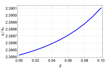
Figure 1: $q/k_{\scriptscriptstyle 0}$ as a function of $\delta$ when medium ${\cal A}$ is crocoite and medium ${\cal B}$ is specified by $\varepsilon_{{\cal B}a}=5.6791$ and $\varepsilon_{{\cal B}b}=\varepsilon_{{\cal B}a}+\delta$. The propagation angle $\psi=31^{\circ}$.

For this example, unexceptional surface waves conforming to Case I exist for $\delta>0$ while an exceptional surface wave conforming to Case II exists for $\delta=0$. For the unexceptional surface waves, the fields in the half-spaces $z>0$ and $z<0$ are specified through Eqs. (2.1.1) and (45), respectively. Equation (52) has be solved for $q$, often numerically using, for example, the Newton–Raphson method [38]. For the exceptional surface wave, the fields in the half-spaces $z>0$ and $z<0$ are specified through Eqs. (37) and (45), respectively. However, Eq. (52) does not have to be solved to determine $q$; instead, $q$ is provided by Eq. (21). In both cases, Eq. (51) has to be manipulated to determine three of the four coefficients in the column 4-vector on the left side in terms of the fourth coefficient.

The relative surface wave number $q/k_{\scriptscriptstyle 0}$ is plotted against $\delta$ in Fig. 1 for $\delta\in\left[0,0.1\right]$. The value of $q/k_{\scriptscriptstyle 0}$ increases uniformly as $\delta$ increases to $0.1$. No surface-wave solutions were found for $\delta>0.1$.

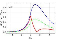
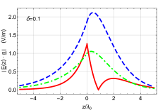
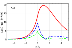
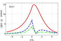
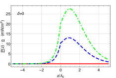
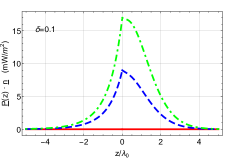
Figure 2: $|\underline{E}(z\hat{\underline{u}}_{z})\mbox{ \tiny{${}^{\bullet}$} }\underline{n}|$, $|\underline{H}(z\hat{\underline{u}}_{z})\mbox{ \tiny{${}^{\bullet}$} }\underline{n}|$, and $\underline{P}(z\hat{\underline{u}}_{z})\mbox{ \tiny{${}^{\bullet}$} }\underline{n}$ plotted versus $z/\lambda_{\scriptscriptstyle 0}$, when medium ${\cal A}$ is crocoite and medium ${\cal B}$ is specified by $\varepsilon_{{\cal B}a}=5.6791$ and $\varepsilon_{{\cal B}b}=\varepsilon_{{\cal B}a}+\delta$. The propagation angle $\psi=31^{\circ}$. (left) $\delta=0$ for which $q=2.3894k_{\scriptscriptstyle 0}$; (right) $\delta=0.1$ for which $q=2.3901k_{\scriptscriptstyle 0}$. Normalization is such that $|\underline{E}(\underline{0})\mbox{ \tiny{${}^{\bullet}$} }\hat{\underline{u}}_{x}|=1$ V m^-1. Key: $\underline{n}=\hat{\underline{u}}_{x}$ (green broken dashed curves), $\underline{n}=\hat{\underline{u}}_{y}$ (blue dashed curves), and $\underline{n}=\hat{\underline{u}}_{z}$ (red solid curves).

Figure 2 shows the magnitudes of the Cartesian components of the electric field phasor $\underline{E}(\underline{r})$, magnetic field phasor $\underline{H}(\underline{r})$, and the time-averaged Poynting vector

$$\underline{P}(\underline{r})=(1/2){\rm Re}\left\{\underline{E}(\underline{r})\times\underline{H}^{\ast}(\underline{r})\right\}$$ (53)

on the $z$ axis for

• the exceptional surface wave existing at $\delta=0$ and

• the unexceptional surface wave existing at $\delta=0.1$.

There are marked differences in the localizations of these two surface waves: The exceptional surface wave is more tightly localized to the interface than the unexceptional surface wave in medium ${\cal B}$ (i.e., $z<0$), whereas the unexceptional surface wave is more tightly localized to the interface than the exceptional surface wave in medium ${\cal A}$ (i.e., $z>0$). The maximum energy density flow for the unexceptional surface wave occurs at $z=0$ while the maximum for the exceptional surface wave occurs in the vicinity of $z\approx 0.9\lambda_{\scriptscriptstyle 0}$ (in medium ${\cal A}$).

In order to consider an exceptional surface wave conforming to Case III next, we set $\varepsilon_{{\cal A}a}=5.6$, $\varepsilon_{{\cal A}b}=\varepsilon_{{\cal A}a}+\delta$, $\varepsilon_{{\cal A}c}=\varepsilon_{{\cal A}a}-\delta$, $\varepsilon_{{\cal B}a}=5$, and $\varepsilon_{{\cal B}b}=17$. As previously, $\delta\geq 0$. The propagation angle $\psi$ is fixed at $19.1183^{\circ}$.

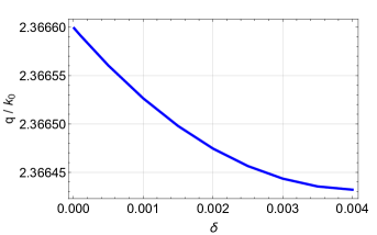
Figure 3: $q/k_{\scriptscriptstyle 0}$ as a function of $\delta$ when medium ${\cal A}$ is specified by $\varepsilon_{{\cal A}a}=5.6$, $\varepsilon_{{\cal A}b}=\varepsilon_{{\cal A}a}+\delta$, and $\varepsilon_{{\cal A}c}=\varepsilon_{{\cal A}a}-\delta$, and medium ${\cal B}$ is specified by $\varepsilon_{{\cal B}a}=5$ and $\varepsilon_{{\cal B}b}=17$. The propagation angle $\psi=19.1183^{\circ}$.

For this example, unexceptional surface waves conforming to Case I exist for $\delta>0$ while an exceptional surface wave conforming to Case III exists for $\delta=0$. For the exceptional surface wave, the fields in the half-spaces $z>0$ and $z<0$ are specified through Eqs. (2.1.1) and (50), respectively. Again, Eq. (52) does not have to be solved to determine $q$ for the exceptional surface wave; instead $q$ is provided by Eq. (47). Thereafter, Eq. (51) has to be manipulated to determine three of the four coefficients in the column 4-vector on the left side in terms of the fourth coefficient.

In Fig. 3, the graph of the relative surface wave number $q/k_{\scriptscriptstyle 0}$ versus $\delta$ is displayed for $\delta\in\left[0,0.004\right]$. The value of $q/k_{\scriptscriptstyle 0}$ decreases uniformly as $\delta$ increases. No surface-wave solutions were found for $\delta>0.004$.

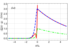
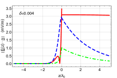
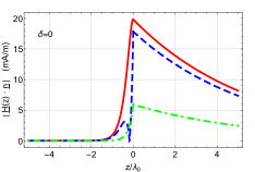
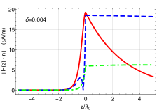
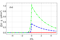
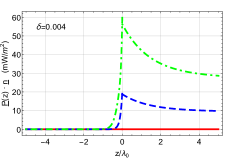
Figure 4: $|\underline{E}(z\hat{\underline{u}}_{z})\mbox{ \tiny{${}^{\bullet}$} }\underline{n}|$, $|\underline{H}(z\hat{\underline{u}}_{z})\mbox{ \tiny{${}^{\bullet}$} }\underline{n}|$, and $\underline{P}(z\hat{\underline{u}}_{z})\mbox{ \tiny{${}^{\bullet}$} }\underline{n}$ plotted versus $z/\lambda_{\scriptscriptstyle 0}$, when medium ${\cal A}$ is specified by $\varepsilon_{{\cal A}a}=5.6$, $\varepsilon_{{\cal A}b}=\varepsilon_{{\cal A}a}+\delta$, and $\varepsilon_{{\cal A}c}=\varepsilon_{{\cal A}a}-\delta$, and medium ${\cal B}$ is specified by $\varepsilon_{{\cal B}a}=5$ and $\varepsilon_{{\cal B}b}=17$. The propagation angle $\psi=19.1183^{\circ}$. (left) $\delta=0$ for which $q=2.36660k_{\scriptscriptstyle 0}$; (right) $\delta=0.004$ for which $q=2.36642k_{\scriptscriptstyle 0}$. Normalization is such that $|\underline{E}(z\hat{\underline{u}}_{z})\mbox{ \tiny{${}^{\bullet}$} }\hat{\underline{u}}_{x}|=1$ V m^-1. Key: $\underline{n}=\hat{\underline{u}}_{x}$ (green broken dashed curves), $\underline{n}=\hat{\underline{u}}_{y}$ (blue dashed curves), and $\underline{n}=\hat{\underline{u}}_{z}$ (red solid curves).

Profiles of $\underline{E}(z\hat{\underline{u}}_{z})$, $\underline{H}(z\hat{\underline{u}}_{z})$, and $\underline{P}(z\hat{\underline{u}}_{z})$ are presented in Fig. 4 for

• the exceptional surface wave existing at $\delta=0$ and

• the unexceptional surface wave existing at $\delta=0.004$.

The profiles for the two surface waves are qualitatively similar but differences in the degree of localization are apparent: The exceptional surface wave is more tightly localized to the interface than the unexceptional surface wave in medium ${\cal A}$ (i.e., $z>0$), whereas the degree of localization in medium ${\cal B}$ (i.e., $z<0$) is approximately the same for the unexceptional and exceptional surface waves.

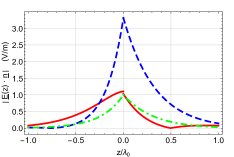
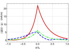
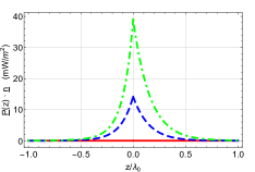
Figure 5: $|\underline{E}(z\hat{\underline{u}}_{z})\mbox{ \tiny{${}^{\bullet}$} }\underline{n}|$, $|\underline{H}(z\hat{\underline{u}}_{z})\mbox{ \tiny{${}^{\bullet}$} }\underline{n}|$, and $\underline{P}(z\hat{\underline{u}}_{z})\mbox{ \tiny{${}^{\bullet}$} }\underline{n}$ plotted versus $z/\lambda_{\scriptscriptstyle 0}$, when medium ${\cal A}$ is crocoite and medium ${\cal B}$ is specified by $\varepsilon_{{\cal B}a}=5.25$ and $\varepsilon_{{\cal B}b}=8.4379$. The propagation angle $\psi=16.4480^{\circ}$ and the relative wavenumber $q=2.3891k_{\scriptscriptstyle 0}$. Normalization is such that $|\underline{E}(z\hat{\underline{u}}_{z})\mbox{ \tiny{${}^{\bullet}$} }\hat{\underline{u}}_{x}|=1$ V m^-1. Key: $\underline{n}=\hat{\underline{u}}_{x}$ (green broken dashed curves), $\underline{n}=\hat{\underline{u}}_{y}$ (blue dashed curves), and $\underline{n}=\hat{\underline{u}}_{z}$ (red solid curves).

Lastly, we turn to Case IV, i.e., the case of a doubly exceptional surface wave. For this purpose, we again take medium ${\cal A}$ to be crocoite in its orthorhombic form while medium ${\cal B}$ is specified by the relative permittivity parameters $\varepsilon_{{\cal B}a}=5.2500$ and $\varepsilon_{{\cal B}b}=8.4379$. The propagation angle $\psi=16.4480^{\circ}$. In this case the surface wavenumber $q$ must simultaneously satisfy Eqs. (21) and (47); its value is $q=2.3891k_{\scriptscriptstyle 0}$. The spatial profiles of the field phasors available from from Eq. (51) are plotted in Fig. 5. These spatial profiles are qualitatively and quantitatively different from those for the exceptional surface waves in Figs. 2 and 4. Specifically, the doubly exceptional surface wave is very tightly bound to the interface, being largely confined to the region $|{z}|<\lambda_{\scriptscriptstyle 0}$. Also, the energy density flow for the doubly exceptional surface wave is approximately symmetric across the bimedium interface $z=0$, in contrast to that for the exceptional surface waves in Figs. 2 and 4.

Unlike the exceptional surface waves (Cases II and III), the doubly exceptional surface wave arises as an isolated degeneracy in the space of the constitutive parameters and propagation angle. That is, if the constitutive parameters or the propagation angle that yield a doubly exceptional surface wave are varied slightly, even by a minuscule amount (say $<0.0001\%$), then no surface-wave solutions can be found.

4 Concluding Remarks

The planar interface of two dissimilar homogeneous dielectric mediums can guide exceptional surface waves when one of the two partnering mediums is anisotropic while the other is isotropic (but we note that other constitutive contrasts between the two partnering mediums may also allow exceptional surface waves to exist). Exceptional surface waves are distinguished from unexceptional surface waves by their unique localization characteristics in the anisotropic partnering medium. If both partnering mediums are anisotropic, we have shown here that a doubly exceptional surface wave could exist for an isolated propagation direction. Doubly exceptional surface waves are distinguished from unexceptional surface waves and exceptional surface waves by their unique localization characteristics in both partnering mediums.

The numerical demonstration of a doubly exceptional surface wave presented herein was based on anisotropic partnering mediums characterized by physically realizable constitutive parameters. Furthermore, our numerical studies revealed that the doubly exceptional surface wave arises as an isolated degeneracy in the space of the constitutive parameters and the propagation direction; i.e., the doubly exceptional surface wave is enclosed by null surface-wave solutions in the space of the constitutive parameters and the propagation direction.

Acknowledgments. This work was supported in part by EPSRC (grant number EP/S00033X/1) and US NSF (grant number DMS-1619901). AL thanks the Charles Godfrey Binder Endowment at the Pennsylvania State University for partial support of his research endeavors.

Disclosures. The authors declare no conflicts of interest.

References

- [1] J. Billard, Contribution a l’Etude de la Propagation des Ondes Electromagnetiques Planes dans Certains Milieux Materiels (2ème these) (Ph.D. Thesis, Université de Paris 6, France, 1966); pp. 175–178.
- [2] D.W. Berreman, “Optics in stratified and anisotropic media: 44-matrix formulation,” J. Opt. Soc. Am. 62, 502–510 (1972).
- [3] T.G. Mackay and A. Lakhtakia, The Transfer-Matrix Method in Electromagnetics and Optics (Morgan & Claypool, 2020).
- [4] M.C. Pease III, Methods of Matrix Algebra (Academic Press, 1965).
- [5] A.L. Shuvalov and P. Chadwick, “Degeneracies in the theory of plane harmonic wave propagation in anisotropic heat-conducting elastic media,” Philos. Trans. R. Soc. Lond. A 355, 156–188 (1997).
- [6] T.G. Mackay and A. Lakhtakia, Electromagnetic Anisotropy and Bianisotropy: A Field Guide, 2nd Edition (World Scientific, 2019).
- [7] G.N. Borzdov, “Waves with linear, quadratic and cubic coordinate dependence of amplitude in crystals,” Pramana–J. Phys. 46, 245–257 (1996) .
- [8] J. Gerardin and A. Lakhtakia, “Conditions for Voigt wave propagation in linear, homogeneous, dielectric mediums,” Optik 112, 493–495 (2001).
- [9] M. Grundmann, C. Sturm, C. Kranert, S. Richter, R. Schmidt-Grund, C. Deparis, and J. Zúiga-Pérez, “Optically anisotropic media: New approaches to the dielectric function, singular axes, microcavity modes and Raman scattering intensities,” Phys. Stat. Sol. RRL 11, 1600295 (2017).
- [10] W. Voigt, “On the behaviour of pleochroitic crystals along directions in the neighbourhood of an optic axis,” Phil. Mag. 4, 90–97 (1902).
- [11] S. Pancharatnam, “Light propagation in absorbing crystals possessing optical activity — Electromagnetic theory,” Proc. Ind. Acad. Sci. A 48, 227–244 (1958).
- [12] A. Brenier, “Voigt wave investigation in the KGd(WO4)2:Nd biaxial laser crystal,” J. Opt. (Bristol) 17, 075603 (2015).
- [13] T.G. Mackay, “Controlling Voigt waves by the Pockels effect,” J. Nanophoton. 9, 093599 (2015).
- [14] N. Moiseyev, Non-Hermitian Quantum Mechanics (Cambridge Univ. Press, 2011).
- [15] W.D. Heiss, “The physics of exceptional points,” J. Phys. A: Math. Theor. 45, 444016 (2012).
- [16] N. Moiseyev and S. Friedland, “Association of resonance states with the incomplete spectrum of finite complex-scaled Hamiltonian matrices,” Phys. Rev. A 22, 618–624 (1980).
- [17] T.G. Mackay and A. Lakhtakia, “On the propagation of Voigt waves in energetically active materials,” Eur. J. Phys. 37, 064002 (2016).
- [18] J.A. Polo Jr., T.G. Mackay, and A. Lakhtakia, Electromagnetic Surface Waves: A Modern Perspective (Elsevier, 2013).
- [19] A.D. Boardman (Ed.), Electromagnetic Surface Modes (Wiley, 1982).
- [20] K. Uller, Beiträge zur Theorie der Elektromagnetischen Strahlung (Ph.D. Thesis, Universität Rostock, Germany, 1903); Chapter XIV.
- [21] J. Zenneck, “Über die Fortpflanzung ebener elektromagnetischer Wellen längs einer ebenen Lieterfläche und ihre Beziehung zur drahtlosen Telegraphie,” Ann. Phys. Lpz. 23, 846–866 (1907).
- [22] M. Faryad and A. Lakhtakia, “Observation of the Uller–Zenneck wave,” Opt. Lett. 39, 5204–5207 (2014).
- [23] G.J. Sprokel, “The reflectivity of a liquid crystal cell in a surface plasmon experiment,” Mol. Cryst. Liq. Cryst. 68, 39–45 (1981).
- [24] A.N. Fantino, “Planar interface between a chiral medium and a metal: surface wave excitation,” J. Modern Opt. 43, 2581–2593 (1996).
- [25] H.-F. Zhang, Q. Wang, N.-H. Shen, R. Li, J. Chen, J. Ding, and H.-T. Wang, “Surface plasmon polaritons at interfaces associated with artificial composite materials,” J. Opt. Soc. Am. B 22, 2686–2696 (2005).
- [26] M. Durach, “Complete 72-parametric classification of surface plasmon polaritons in quartic metamaterials,” OSA Continuum 1, 162–169 (2018).
- [27] F.N. Marchevskiĭ, V.L. Strizhevskiĭ, and S.V. Strizhevskiĭ, “Singular electromagnetic waves in bounded anisotropic media,” Sov. Phys. Solid State 26, 911–912 (1984).
- [28] M.I. D’yakonov, “New type of electromagnetic wave propagating at an interface,” Sov. Phys. JETP 67, 714–716 (1988).
- [29] O. Takayama, L. Crasovan, D. Artigas, and L. Torner, “Observation of Dyakonov surface waves,” Phys. Rev. Lett. 102, 043903 (2009).
- [30] A.N. Furs and L.M. Barkovsky, “Surface polaritons at the planar interface of twinned dielectric gyrotropic media,” Electromagnetics 28, 146–161 (2008).
- [31] T.G. Mackay and A. Lakhtakia, “Temperature-mediated transition from Dyakonov surface waves to surface-plasmon-polariton waves,” IEEE Photon. J. 8, 4802813 (2016).
- [32] O. Takayama, L.C. Crasovan, S.K. Johansen, D. Mihalache, D. Artigas, and L. Torner, “Dyakonov surface waves: a review,” Electromagnetics 28, 126–145 (2008).
- [33] C. Zhou, T.G. Mackay, and A. Lakhtakia, “Surface-plasmon-polariton wave propagation supported by anisotropic materials: Multiple modes and mixed exponential and linear localization characteristics,” Phys. Rev. A 100, 033809 (2019).
- [34] T.G. Mackay, C. Zhou, and A. Lakhtakia, “Dyakonov–Voigt surface waves,” Proc. R. Soc. A 475, 20190317 (2019).
- [35] C. Zhou, T.G. Mackay, and A. Lakhtakia, “On Dyakonov–Voigt surface waves guided by the planar interface of dissipative materials,” J. Opt. Soc. Amer. B 36, 3218–3225 (2019).
- [36] J.F. Nye, Physical Properties of Crystals: Their Representation by Tensors and Matrices. (Oxford University Press, 1985).
- [37] W.E. Boyce and R.C. DiPrima, Elementary Differential Equations and Boundary Value Problems, 9th Edition (Wiley, 2010).
- [38] Y. Jaluria, Computer Methods for Engineering (Taylor & Francis, 1996).
- [39] G. Collotti, L. Conti, and M. Zocchi, “The structure of the orthorhombic modification of lead chromate PbCrO4,” Acta Cryst. 12, 416 (1959).