Confined nano-NMR spectroscopy using NV centers

Abstract

Nano-NMR spectroscopy with nitrogen-vacancy centers holds the potential to provide high resolution spectra of minute samples. This is likely to have important implications for chemistry, medicine and pharmaceutical engineering. One of the main hurdles facing the technology is that diffusion of unpolarized liquid samples broadens the spectral lines thus limiting resolution. Experiments in the field are therefore impeded by the efforts involved in achieving high polarization of the sample which is a challenging endeavor. Here we examine a scenario where the liquid is confined to a small volume. We show that the confinement ’counteracts’ the effect of diffusion, thus overcoming a major obstacle to the resolving abilities of the NV-NMR spectrometer.

I INTRODUCTION

Nano Nuclear Magnetic Resonance (nano-NMR) spectroscopy is a new field that aimes to implement methods similar to classic NMR techniques on minute samples. The new technology may outperform microscopy methods and enable high resolution imaging at the single molecule level. Therefore, advances in the field will have major implications for fundamental science and pave the way for drug and medicine development.

Scaling down the sample size requires a different measurement device, because small samples generate magnetic fields that are undetectable by classical sensors. The Nitrogen-Vacancy (NV) center based spectrometer is a promising platform for nano-NMR, since the NV is a superb magnetometer of small fields Jensen et al. (2017); Doherty et al. (2013). Although many successful experiments using the NV spectrometer have been carried out in recent years DeVience et al. (2015); Mamin et al. (2013); Shagieva et al. (2018a); Pfender et al. (2019); Aslam et al. (2017), nearly all of them used a large sample size to generate a reasonable signal. The gain from using large volumes has to do with the dipolar interaction between the sensor and the nuclear spin ensemble. This creates an effective cut-off distance which is proportional to the NV’s depth $d$, such that only nuclei within a radius of $\sim d$ from the surface contribute to the magnetic field. This limitation suggests that a resolution problem occurs when using shallow NVs since the diffusion time across the detection volume which sets the resolution capability is shorter (see Fig. 1a).

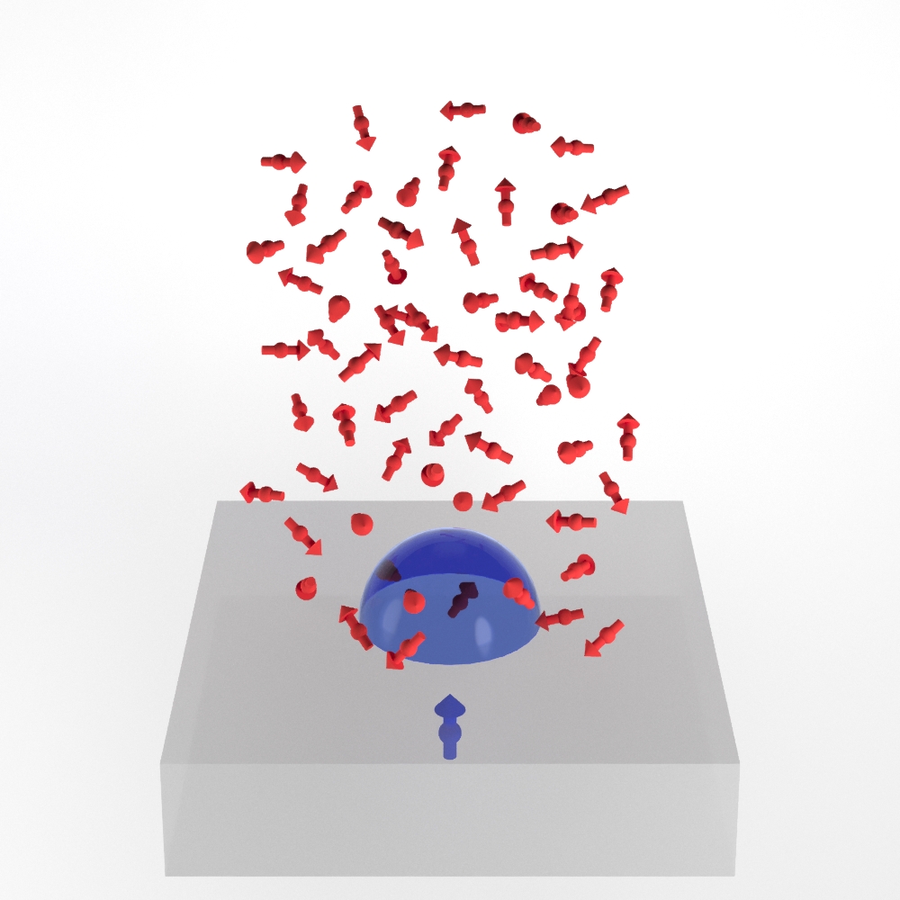
(a)

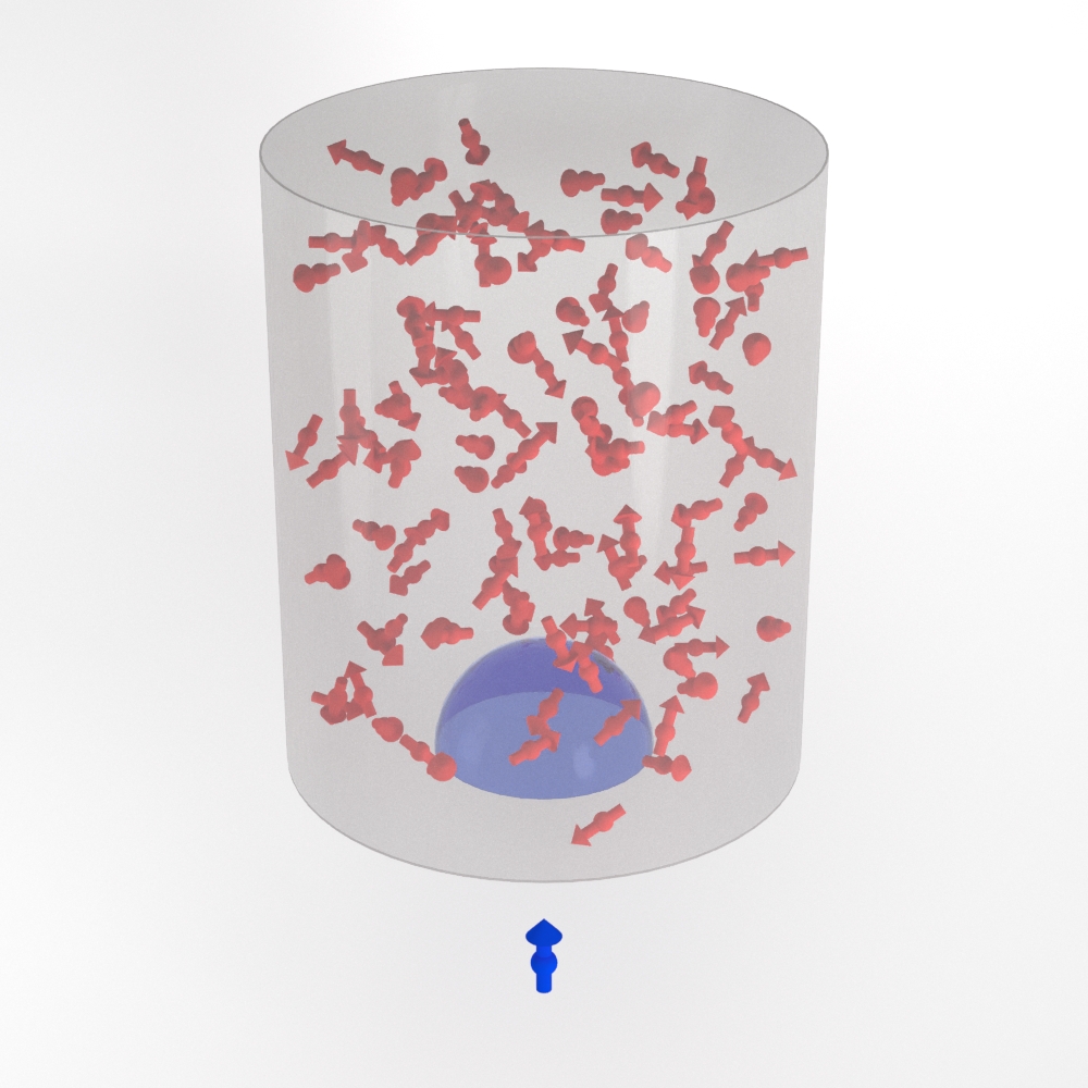
(b)

Figure 1: (a) Nano-NMR using NV centers - the nuclear spin sample (red arrows) is placed on top of a diamond surface. The ensemble interacts with the NV center (blue arrow), which is situated at a distance $d$ below the surface. The dioplar interaction creates an effective cutoff, such that only spins that are found in a hemisphere of radius $\sim d$ (blue dome) contribute to the magnetic field at the NV’s position. While the generated field of the statistically polarized spins provides information about their Larmor frequency, after interrogation times $t>\tau_{D}\equiv\frac{d^{2}}{D}$, the diffusion of spins outside the effective interaction region causes the field to fluctuate, which eventually leads to the decohernce of the sensor. This results in a resolution problem in nano-NMR using shallow sensors. (b) Confined nano-NMR - the nuclear spin ensemble is confined to a small space (gray cylinder). For interrogation times $t<\tau_{V}\equiv\frac{V^{2/3}}{D}$ the dynamics is similar to the non-confined scenario, since the interaction with the walls in negligible. For times $t>\tau_{V}$, however, the nuclei have a finite probability of returning to the interaction volume, which leads to non-vanishing correlations of the magnetic field. These figures were created by Bar Soffer, Mirage studio.

One way of avoiding the resolution problem is by using an ultra-polarized sample. While some experiments rely solely on statistical polarization, other types of polarizations; e.g. thermal polarization or hyperpolarized non-equilibrium states can be used to amplify the signal and circumvent the effects of diffusion Glenn et al. (2018); Bucher et al. (2018). It was also shown that given high polarization, the entanglement formed between the shallow sensors and the nuclear spin ensemble can be utilized to further increase precision Cohen et al. (2019). However, despite considerable efforts to enhance the sample’s polarization, current state-of-the art achieves about $1\%$. Going beyond this requires efficient hyperpolarization schemes which are technically hard to implement. Recent works suggest practical alternatives by showing that contrary to common assumptions, diffusion noise can be managed by implementing an appropriate measurement protocol. These methods rely on the long lasting correlation of magnetic field noise in liquid state nano-NMR with NV centers Cohen et al. (2020); Rotem et al. .

Another elegant and practical approach that is currently being explored by the community is to confine the nuclei in a small volume, thus limiting the effects of diffusion (see Fig. 1b). Here we provide a detailed theoretical analysis of confined nano-NMR spectroscopy. We calculate the expected average magnetic field and correlations in three different geometries: a cylinder, a hemisphere and a full sphere. We show that for any geometry of volume $V$ the correlations decay to a constant value, resulting in unlimited resolution and an SNR which is a fraction of $\sim\frac{d^{3}}{V}$ from the SNR of the power spectrum at low frequency.

The advantage of confinement can easily be understood by the following argument. Denoting the liquid’s diffusion coefficient by $D$, keep in mind that the system has two characteristic time scales: the time it takes a nucleus to diffuse out of the effective interaction region, $\tau_{D}=\frac{d^{2}}{D}$, and the time it takes a nucleus to reach the volume’s boundary, $\tau_{V}=\frac{V^{2/3}}{D}$. Assuming that $d<V^{1/3}$, we expect that for short times, $t<\tau_{D}=\frac{d^{2}}{D}$, when nuclei can rarely leave the interaction region, the magnetic field at the NV’s position will be approximately constant. Therefore, the correlation is also constant. For intermidiate times $\tau_{D}<t$, as diffusion becomes dominant, the fluctuations in the magnetic field will cause the correlations to decay, while for $\tau_{D}\ll t\ll\tau_{V}$ the correlation will decay as a power law Cohen et al. (2020). However, for longer times $t>\tau_{V}$, nuclei are reflected from the boundary and therefore have a finite probability to return to the interaction region, which causes the correlation to decay to a constant value. The probability can be estimated by the ratio of the effective interaction region and the total volume $\sim\frac{d^{3}}{V}$. The expected form of the correlation function is sketched in Fig. 2. In the following, we show in detail that these simple arguments indeed describe the correlation of confined nano-NMR.

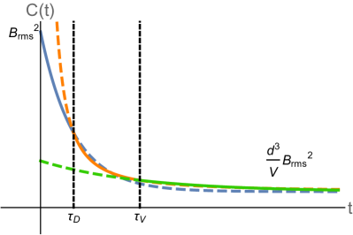
Figure 2: A sketch of the expected behavior of the correlation function. Solid lines represent the approximate behavior in each regime, and dashed lines are extensions of the approximations to regimes where they are invalid. The value of the correlation at $t=0$ is defined as $B_{rms}^{2}$. For times $t\ll\tau_{D}$ the correlation decays exponentially, which is approximately linear for small arguments (blue line). As diffusion becomes dominant at times $t>\tau_{D}$ the exponential scaling is no longer valid (dashed blue line) and it changes to a power law $\propto t^{-3/2}$ (orange line). When the nuclei interact with the walls at times $t>\tau_{V}$ the correlation decays exponentially to a constant $\sim\frac{d^{3}}{V}B_{rms}^{2}$.

II RESULTS

II.1 Measurement protocol

We explore two measurement schemes: correlation spectroscopy Staudacher et al. (2015); Kong et al. (2015); Laraoui et al. (2013); Rosskopf et al. (2017); Zaiser et al. (2016) and a phase sensitive measurement (Qdyne) Schmitt et al. (2017); Boss et al. (2017); Glenn et al. (2018). In the following we provide an outline of the two. We consider the NV center as a two level system (spin $\frac{1}{2}$) with an energy gap of $\gamma_{e}B_{ext}$, where $B_{ext}$ is the externally applied magnetic field and $\gamma_{e/n}$ is the electron/nuclei gyromagntic ratio Doherty et al. (2013). We denote $S_{i}\ (I_{i})$ as the spin operator of the NV (nuclear spin) at the $i$ direction, $S_{\pm}\ (I_{\pm})$ as the NV’s (nuclear spin’s) raising/lowering operators and $\theta_{i}$ as the angle between the NV’s magnetization axis and the vector connecting the NV to the $i$-th nucleus.

In correlation spectroscopy, the NV interacts with nuclear spins for a period of time $\tau$ via the dipolar interaction with the ensemble at the end of which the NV state is written onto a memory qubit or alternatively the relevant information found in the relative phase is mapped to the population difference of the NV. After a waiting time $t$ the experiment is carried out again for the same period of time $\tau$. At the interrogation times the NV is driven with an external pulse sequence at frequency $\omega_{p}$, which is close to the Larmor frequency of the nuclei $\omega_{N}$, such that $\left(\omega_{N}-\omega_{p}\right)t\equiv\delta t\ll 1$. The Hamiltonian is effectively

$$H_{eff}=\gamma_{e}B(t)S_{z}\cos\left(\delta t+\phi\right),$$ (1)

where $\phi$ is a random phase deriving from the unpolarized dynamics. Initializing the NV in the state $|\psi_{0}\rangle=\frac{1}{\sqrt{2}}\left(|\uparrow\rangle+|\downarrow\rangle\right)$, after both interrogation periods, the probability of measuring the NV at the $|\psi_{0}\rangle$ state is

$$P_{|\psi_{0}\rangle}\approx 1-\left(2\gamma_{e}^{2}\tau\right)^{2}\left[B^{2}\left(0\right)\cos^{2}\left(\phi\right)\right.$$ (2)

$$\left.+B^{2}\left(t\right)\cos^{2}\left(\delta t+\phi\right)+2B\left(0\right)B\left(t\right)\cos\left(\phi\right)\cos\left(\delta t+\phi\right)\right],$$

where we took the weak back-action limit, namely $\gamma_{e}B(t)\tau\ll 1$. Averaging (2) over realizations yields

$$P_{|\psi_{0}\rangle}\approx 1-\left(2\gamma_{e}B_{rms}\tau\right)^{2}\left[1+\cos\left(\delta t\right)\frac{C^{(1)}\left(t\right)}{B_{rms}^{2}}\right],$$ (3)

where $C^{(1)}\left(t\right)=\left<B\right(t\left)B\right(0\left)\right>$ is the correlation function of the magnetic field at time $t$ thus $C\left(0\right)\equiv B_{rms}^{2}$. The correlation is given by Cohen et al. (2020); Sup

$$C^{(m)}\left(t\right)=\tilde{\zeta}_{m}^{2}\int\frac{d^{3}r}{r^{3}}\int\frac{d^{3}r_{0}}{r_{0}^{3}}Y_{2}^{(m)}\left(\Omega\right)Y_{2}^{(m)*}\left(\Omega_{0}\right)P\left(\bar{r},\bar{r}_{0},t\right),$$ (4)

where $Y_{l}^{(m)}$ are the spherical harmonics, $P\left(\bar{r},\bar{r}_{0},t\right)$ is the diffusion propagator from $\bar{r}$ to $\bar{r}_{0}$ with time difference $t$ and $\tilde{\zeta}_{m}$ are defined in Sup . For $m=1$, for example, $\tilde{\zeta}_{1}=\frac{3}{2}\left(2\sqrt{\frac{2\pi}{15}}\right)\left(\frac{\hbar\mu_{0}\gamma_{N}}{4\pi}\right)$. For a detailed derivation of Eq. (3) see Sup . We note that different values of $m$ can be sampled by changing the dynamical decoupling pulse frequency. For example, $m=0$ can be sensed by not applying any pulses ($\omega_{p}=0$).

In a phase sensitive measurement we employ a similar protocol, where the main difference stems from the fact that we measure multiple times in one realization; every period $\tau$ the NV is measured and then initialized at the state $|\psi_{0}\rangle$. The evolution of the system between times $t_{n}\equiv n\tau$ and $t_{n+1}=\left(n+1\right)\tau$ for some integer $n$ is

$$|\psi_{t_{n+1}}\rangle=\frac{1}{\sqrt{2}}\left[\exp\left(-2i\gamma_{e}\tau B\left(t_{n}\right)\cos\left(\delta t_{n}+\phi\right)\right)|\uparrow\rangle+|\downarrow\rangle\right],$$ (5)

where we assumed $\delta\tau\ll 1$. The probability of measuring $|\uparrow_{y}\rangle=\frac{1}{\sqrt{2}}\left(|\uparrow\rangle+i|\downarrow\rangle\right)$ is therefore

$$P_{|\uparrow_{y}\rangle}\left(t_{n}\right)=\frac{1}{2}\left(1+\sin\left[\Phi\left(t_{n}\right)\right]\right)$$ (6)

with $\Phi\left(t_{n}\right)=2\gamma_{e}\tau B\left(t_{n}\right)\cos\left(\delta t_{n}+\phi\right)$. Assuming $\Phi\left(t_{n}\right)\ll 1$ we can approximate (6) by

$$P_{|\uparrow_{y}\rangle}\left(t_{n}\right)\approx\frac{1}{2}\left[1+\Phi\left(t_{n}\right)\right].$$ (7)

The joint probability is then

$$P_{|\uparrow_{y}\rangle}\left(t_{n}\right)P_{|\uparrow_{y}\rangle}\left(t_{k}\right)\approx\frac{1}{4}\left[1+\Phi\left(t_{n}\right)+\Phi\left(t_{k}\right)+\Phi\left(t_{n}\right)\Phi\left(t_{k}\right)\right].$$ (8)

When combined with the probability of both results being $|\downarrow_{y}\rangle$, an extra factor of 2 is gained. Averaging (8) over the different measurements gives

$$\left<P_{|\uparrow_{y}\rangle}\left(t_{n}\right)P_{|\uparrow_{y}\rangle}\left(t_{k}\right)\right>\approx$$ (9)

$$\frac{1}{4}\left[1+\left(2\gamma_{e}\tau\right)^{2}C^{(m)}\left(t_{n-k}\right)\cos\left(\delta t_{n-k}\right)\right].$$

This can be used to define a new Bernoulli variable by

$$P=\left<P_{|\uparrow_{y}\rangle}\left(t_{n}\right)P_{|\uparrow_{y}\rangle}\left(t_{k}\right)\right>+\left<P_{|\downarrow_{y}\rangle}\left(t_{n}\right)P_{|\downarrow_{y}\rangle}\left(t_{k}\right)\right>$$ (10)

$$=\frac{1}{2}\left[1+\left(2\gamma_{e}\tau\right)^{2}C^{(m)}\left(t_{n-k}\right)\cos\left(\delta t_{n-k}\right)\right],$$

where the value of $m$ in Eqs. (9) and (10) is determined by the external pulse frequency. In the following we present the calculation magnetic field correlations in three different geometries. We provide analytic calculations for the asymptotic behavior and numerical assessments for arbitrary times. Since the asymptotic behavior of the correlation functions is universal, we focus on the case $m=0$. The calculation of the other correlation functions can be found in Sup .

II.1.1 Cylinder

Given a statistically polarized ensemble which is confined to a cylinder with height $L$ and radius $R$ and an NV that is located at a depth $d$ below the cylinder’s base. The NV’s position coincides with the cylinder’s symmetry axis denoted as $\hat{z}$. Assuming the NV’s magnetization axis is along the $\hat{z}$ axis, the magnetic field correlation is given by (4), where the different $m$ values can be probed by changing the pulse frequency mentioned in the previous section, see details in Cohen et al. (2020). The instantaneous correlation, $B_{rms}^{2}=C^{(0)}\left(t=0\right)$ can be calculated analytically as the propagator approaches a delta function, yielding:

$$\frac{B_{rms}^{2}}{J^{2}}=\frac{\pi}{64}\left\{\frac{1}{R^{2}}\left[\frac{23d}{d^{2}+R^{2}}+\frac{24d^{5}}{\left(d^{2}+R^{2}\right)^{3}}\right.\right.$$ (11)

$$+\frac{16LR^{2}\left(3d^{2}+3dL+L^{2}\right)}{d^{3}(d+L)^{3}}-\frac{38d^{3}}{\left(d^{2}+R^{2}\right)^{2}}$$

$$\left.-\frac{23(d+L)}{(d+L)^{2}+R^{2}}+\frac{38(d+L)^{3}}{\left((d+L)^{2}+R^{2}\right)^{2}}-\frac{24(d+L)^{5}}{\left((d+L)^{2}+R^{2}\right)^{3}}\right]$$

$$+\frac{1}{R^{3}}\left[105\tan^{-1}\left(\frac{R}{d+L}\right)+96\tan^{-1}\left(\frac{d+L}{R}\right)\right.$$

$$\left.\left.-105\tan^{-1}\left(\frac{R}{d}\right)-96\tan^{-1}\left(\frac{d}{R}\right)\right]\right\},$$

where we denote the physical coupling constant by $J=\left(\frac{\hbar\mu_{0}\gamma_{N}}{4\pi}\right)$. Eq. (11) reproduces the well-known scaling, $B^{2}_{rms}\propto J^{2}d^{-3}$, of the semi-infinite volume in the limit $d\ll R,L$, as expected. In the other limit, $d\gg R,L$, Eq. (11) can be approximated by $B^{2}_{rms}\propto J^{2}\frac{V}{d^{6}}$. This is because as the statistical polarization scales as $\sqrt{V}$, the dipole-dipole interaction decays as $\frac{1}{d^{3}}$ and ${B_{RMS}}$ scales with both.

The correlation (4) decays asymptotically to a constant as the propagator approaches the uniform distribution for times $t\gg\tau_{V}$,

$$\frac{C^{(0)}(t\gg\tau_{V})}{J^{2}}\approx\frac{4\pi^{2}}{V}\left(\frac{L+d}{\sqrt{\left(L+d\right)^{2}+R^{2}}}-\frac{d}{\sqrt{d^{2}+R^{2}}}\right)^{2}.$$ (12)

For a sufficiently shallow sensor, $d\ll R,L$ Eq. (12) approaches $C^{(0)}\propto B^{2}_{rms}\frac{d^{3}}{V}=\frac{J^{2}}{V}$. The factor of $\frac{d^{3}}{V}$ in this limit can be interpreted as the probability that a nucleus will be found in the effective interaction region, because at long times, diffusion spreads out the nuclei uniformly. Since the signal $B_{rms}^{2}\propto d^{-3}$, remarkably, the correlation does not depend on the NV’s depth. This regime ($t\gg\tau_{V}$), where the signal remains constant, is reminiscent of the situation of the unbounded region with a polarized sample, wherein the constant correlation is replaced by the average magnetic field.

At arbitrary times, (4) is given by

$$\tilde{C}^{(m)}=\frac{d^{3}}{V}\sum_{s=1}^{\infty}\sum_{k=0}^{\infty}\frac{2}{J_{m}^{2}\left(\nu_{s,m}\right)\left(1-\left(\frac{m}{\nu_{s,m}}\right)^{2}\right)\left(1+\delta_{k,0}\right)}\times$$ (13)

$$e^{-t/\tau_{s,k,m}}\left[\int\frac{d^{3}r}{r^{3}}\cos\left[\pi k\left(\frac{z-d}{L}\right)\right]J_{m}\left(\nu_{s,m}\frac{\rho}{R}\right)\left|Y_{2}^{(m)}\left(\Omega\right)\right|\right]^{2},$$

where $\tilde{C}^{(m)}=\frac{\left[C^{(m)}(t)-C^{(m)}(t\gg\tau_{V})\right]}{C^{(m)(0)}}$, $J_{m}$ is the $m$th Bessel function of the first kind, $\nu_{k,m}$ is the $k$th zero of $J_{m}^{\prime}$, $\delta_{i,j}$ is Kronecker’s delta and the characteristic decay time $\tau_{s,k,m}=\left[D\left(\frac{\nu_{s,m}}{R}\right)^{2}+D\left(\frac{\pi k}{L}\right)^{2}\right]^{-1}$. Note that while Eq. (4) might be very hard to estimate even numerically, Eq. (13) only contains a sum over two dimensional integrals (since the azimuthal integration is trivial) which are easy to calculate.

We evaluated (13) for $k,s\in[1,25]$, the diffusion coefficient of immersion oil $D=0.5\ \frac{\textrm{nm}^{2}}{\mu\textrm{s}}$, $d=1\ \textrm{nm}$ and different volumes Sup . In Fig 3 we present a representative case where $R=L=200\ \textrm{nm}$. The correlation at short times decays linearly, which agrees with an exponential decay for small arguments. In the intermediate regime the decays changes to a power law $\sim t^{-1.5}$ as predicted in previous works Cohen et al. (2020), while at long times the decay rate fits the slowest decaying mode of (13).

The numerical integration was done with a diffusion coefficient fitting immersion oil, since state-of-the-art experiments are conducted with high viscous fluids primarily for their long diffusion time, which results in a long correlation time and thus a high resolution capability. For water, for example, resolution is extremely limited, since the correlation vanishes rapidly. In a confined setting, however, the correlation decays rapidly to a constant value; therefore, diffusion poses no real limitation on the interrogation time thus eliminating the need to use high viscous fluids.

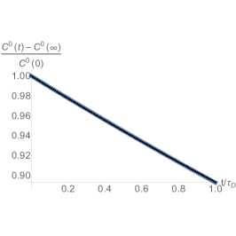
(a)

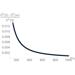
(b)

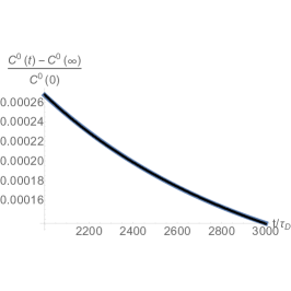
(c)

Figure 3: The correlation function in cylindrical geometry (13) (black points) for $m=0$ in the three time regimes - (a) $t\ll\tau_{D}$, (b) $\tau_{D}\ll t\ll\tau_{V}$ and (c) $\tau\gg\tau_{V}$ (right) . The correlation was calculated for $d=1\ \textrm{nm},\ D=0.5\ \frac{\textrm{nm}^{2}}{\mu\textrm{s}}$ and $R=L=200\ \textrm{nm}$. The short times limit was fitted to a linear function, the intermediate times to a power law and long times were fitted to an exponential function (blue lines). The power in the intermediate regime fit the expected $-1.5$ scaling predicted in previous works, and the decay rate at long times fit the slowest decaying mode of (13).

II.1.2 Hemisphere

The $B_{rms}$ of a hemisphere with radius $R$, given by the limit $t\rightarrow 0$ of Eq. (4) is

$$\frac{B_{rms}^{2}}{J^{2}}=\frac{\pi}{32d^{5}}\left[\left(d^{2}-9R^{2}\right)\ln\left(\frac{d^{2}+R^{2}}{\left(d+R\right)^{2}}\right)\right.$$ (14)

$$+2d^{3}\left(-\frac{5d}{d^{2}+R^{2}}-\frac{4d^{2}}{(d+R)^{3}}-\frac{6d^{5}}{\left(d^{2}+R^{2}\right)^{3}}\right.$$

$$\left.\left.+\frac{2d^{3}}{\left(d^{2}+R^{2}\right)^{2}}+\frac{2d}{(d+R)^{2}}-\frac{2}{d+R}\right)+26d^{2}-18dR\right].$$

The limits of (14) are similar to those of the cylindrical case. The asymptotic behavior at long times is

$$\frac{C^{(0)}(t\gg\tau_{V})}{J^{2}}\approx\frac{4\pi^{2}}{9V}\left[2-\frac{2d}{\sqrt{d^{2}+R^{2}}}\right.$$ (15)

$$\left.-\frac{R^{2}}{d\sqrt{d^{2}+R^{2}}}-\frac{2R^{3}}{d^{3}}\left(\frac{R}{\sqrt{d^{2}+R^{2}}}-1\right)\right]^{2}.$$

Taking $d\ll R$, Eq. (15) reduces to $\frac{16\pi^{2}}{9V}\propto B_{rms}^{2}\frac{d^{3}}{V}$. In general the correlation can be expressed by the sum

$$\tilde{C}^{(m)}=\frac{d^{3}}{V}\sum_{l=0}^{\infty}\sum_{k=1}^{\infty}\frac{4\pi\left[1+\left(-1\right)^{l+m}\right]}{3j_{l}^{2}\left(\tilde{\nu}_{k,l}\right)\left(1-\left(\frac{l}{\tilde{\nu}_{k,l}}\right)^{2}\right)}\times$$ (16)

$$\left[\int\frac{d^{3}r}{\tilde{r}^{3}}j_{l}\left(\frac{\tilde{\nu}_{k,l}}{R}r\right)Y_{2}^{(m)*}\left(\tilde{\theta},\tilde{\phi}\right)Y_{l}^{(m)}\left(\theta,\phi\right)\right]^{2}\exp\left(-\frac{\tilde{\nu}_{k,l}^{2}}{\tau_{V}}t\right),$$

where $j_{m}$ is the $m$th spherical Bessel function of the first kind and $\tilde{\nu}_{k,m}$ is the $k$th zero that does not equal zero of $j_{m}^{\prime}$ (namely, $\tilde{\nu}_{1,m}\neq 0$). The coordinates $\bar{r}/\bar{\tilde{r}}$ are the spherical coordinates where the origin is found at the center of the hemisphere’s base  at the NV’s position. The results are similar to those of the cylindrical geometry and are found in Sup .

II.2 Full sphere

Given a spherical geometry of radius $R$, the instantaneous correlation is

$$\frac{B_{rms}^{2}}{J^{2}}=\frac{\pi}{8d^{3}(d+R)^{5}(d+2R)^{3}}\left[d^{3}\left(-d^{5}-8d^{4}R-16d^{3}R^{2}\right.\right.$$ (17)

$$\left.+16d^{2}R^{3}+80dR^{4}+64R^{5}\right)\tanh^{-1}\left(\frac{R}{d+R}\right)+d^{7}R$$

$$+7d^{6}R^{2}+52d^{5}R^{3}+190d^{4}R^{4}+320d^{3}R^{5}+256d^{2}R^{6}$$

$$\left.+96dR^{7}+16R^{8}\right].$$

The asymptotic behavior of (4) is then given by

$$\frac{C^{(0)}(t\gg\tau_{V})}{J^{2}}\approx\frac{64\pi^{2}}{9V}\frac{R^{6}}{(d+R)^{6}}.$$ (18)

For arbitrary times, the correlation is

$$\tilde{C}^{(m)}=\frac{1}{V}\sum_{l=0}^{\infty}\sum_{k=1}^{\infty}\frac{8\pi}{3j_{l}^{2}\left(\tilde{\nu}_{k,l}\right)\left(1-\left(\frac{l}{\tilde{\nu}_{k,l}}\right)^{2}\right)}\times$$ (19)

$$\left[\int\frac{d^{3}r}{\tilde{r}^{3}}j_{l}\left(\frac{\tilde{\nu}_{k,l}}{R}r\right)Y_{2}^{(m)*}\left(\tilde{\theta},\tilde{\phi}\right)Y_{l}^{(m)}\left(\theta,\phi\right)\right]^{2}\exp\left(-\frac{\tilde{\nu}_{k,l}^{2}}{\tau_{V}}t\right),$$

We evaluated (19) for $l\in[0,30],\ k\in[1,30]$, the diffusion coefficient of immersion oil $D=0.5\ \frac{\textrm{nm}^{2}}{\mu\textrm{s}}$, $d=1\ \textrm{nm}$ and different volumes Sup . In Fig 4 we present a representative case where $R=200\ \textrm{nm}$. The correlation at short times and long times agrees with the results of the cylindrical geometry. In the intermediate regime the decay changes to a power law $\sim t^{-0.5}$.

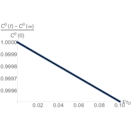
(a)

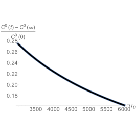
(b)

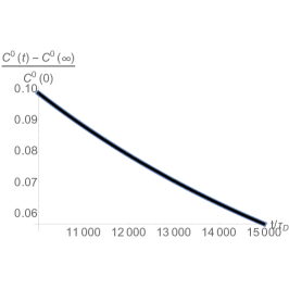
(c)

Figure 4: The correlation function in spherical geometry (19) (black points) for $m=0$ in the three time regimes - (a) $t\ll\tau_{D}$, (b) $\tau_{D}\ll t\ll\tau_{V}$ and (c) $\tau\gg\tau_{V}$ (right) . The correlation was calculated for $d=1\ \textrm{nm},\ D=0.5\ \frac{\textrm{nm}^{2}}{\mu\textrm{s}}$ and $R=L=200\ \textrm{nm}$. The short times limit was fitted to a linear function, the intermediate times to a power law and long times were fitted to an exponential function (blue lines). The results for short times and long times are similar to those of the previous geometries, while the power in the intermediate regime fits a $-0.5$ scaling. (19).

II.3 Sensitivity analysis

In our sensitivity analysis we used the tools of classic parameter estimation. We calculated the Fisher Information (FI), denoted by $\pazocal{I}$; hence, the sensitivity can then be estimated with the Cramer-Rao bound DeGroot and Schervish (2012)

$$\Delta\delta\geq\frac{1}{\sqrt{\pazocal{I}}}.$$ (20)

We start by calculating the asymptotic behavior of the FI in either correlation spectroscopy or a phase sensitive measurement. In the limits $t\leq\tau_{D}$ and $t\gg\tau_{V}$ the correlation is approximately a constant. Note that the regime $t\leq\tau_{D}$ is similar to the unconfined case. The FI of correlation spectroscopy is given by

$$\pazocal{I} = \frac{\left(\frac{dP_{|\Psi_{0}\rangle}}{d\delta}\right)^{2}}{P_{|\Psi_{0}\rangle}\left(1-P_{|\Psi_{0}\rangle}\right)}\frac{T}{t}$$ (21)

$$= \left(2\gamma_{e}t\tau\right)^{2}\left(\frac{C}{B_{rms}}\right)^{2}\frac{\sin^{2}\left(\delta t\right)}{1+\frac{C}{B_{rms}^{2}}\cos\left(\delta t\right)}\frac{T}{t},$$

where $T$ is the total time, and we used Eq. (3) for this derivation. Since $C\left(t\ll\tau_{D}\right)\approx B_{rms}^{2}$ we can deduce that for $t\approx\tau_{D}$,

$$\pazocal{I}_{UCL}\approx 2\left(\gamma_{e}B_{rms}\delta\tau\tau_{D}^{2}\right)^{2}\frac{T}{\tau_{D}}.$$ (22)

Eq. (22) is the unconfined limit (UCL), since without confinement the measurement time is bounded by $\tau_{D}$. For times $t\gg\tau_{V}$, on the other hand, $C\left(t\gg\tau_{V}\right)\approx\frac{d^{3}}{V}B_{rms}^{2}$ and therefore

$$\pazocal{I}_{C}\approx\left(2\gamma_{e}B_{rms}T_{m}\tau\right)^{2}\left(\frac{d^{3}}{V}\right)^{2}\sin^{2}\left(\delta T_{m}\right)\frac{T}{T_{m}},$$ (23)

where $T_{m}$ is the memory time. In the case where $\delta T_{m}>\frac{\pi}{2}$ Eq. (23) can be simplified to

$$\pazocal{I}_{C}\approx\left(2\gamma_{e}B_{rms}\tau\right)^{2}\left(\frac{d^{3}}{V}\right)^{2}T_{m}T.$$ (24)

Comparing Eq. (24) to Eq. (22) shows that we gained a factor of

$$\frac{\pazocal{I}_{C}}{\pazocal{I}_{UCL}}=\frac{T_{m}}{\tau_{D}}\frac{1}{\left(\delta\tau_{D}\right)^{2}}\left(\frac{d^{3}}{V}\right)^{2}.$$ (25)

Since $T_{m}$ can be orders of magnitude larger than $\tau_{D}$ and $\delta\tau_{D}$ might be very small, this can lead to considerable enhancement in sensitivity. Numerical evaluations of Eq. (25) are found at the last section.

In a Qdyne type measurement the probability (10) leads to

$$\pazocal{I}_{s}=16\left(\gamma_{e}\tau\right)^{4}C^{2}\left(t_{s}\right)t_{s}^{2}\sin^{2}\left(\delta t_{s}\right).$$ (26)

For times $t_{s}\gg\tau_{V}$, the Fisher information (26) is

$$\pazocal{I}_{s}=\frac{16\left(\gamma_{e}J\tau\right)^{4}}{V^{2}}t_{s}^{2}\sin^{2}\left(\delta t_{s}\right).$$ (27)

Since the Fisher information is additive and the correlation is always larger than the asymptotic value we can bound the total Fisher information by

$$\pazocal{I}\geq\frac{16\left(\gamma_{e}J\tau\right)^{4}}{V^{2}}\sum_{s=0}^{T/\tau}t_{s}^{2}\sin^{2}\left(\delta t_{s}\right)\approx\frac{8\left(\gamma_{e}J\right)^{4}}{3V^{2}}\tau^{3}T^{3},$$ (28)

where $T$ is the total measurement time. The result (28) is a major improvement over (22), since it scales with $T^{3}$ which is not limited by the diffusion time. The bound (28) is quite crude, since for viscous fluids a great deal of information can be gained from the slow temporal decay. A comprehensive analysis can be found in Rotem et al. .

II.4 Molecular dynamics

We corroborated the analytic prediction of the correlation function of the magnetic field as a result of the fluid motion in the closed geometry using molecular dynamics simulations, focusing on the case of the cylindrical geometry. The set-up is illustrated in figure 5. The system contains $N$ particles, which are confined to a cylinder of radius $R$ and height $L$. The particles interact via the Lennard-Jones (LJ) potential $4\epsilon[(\sigma/r)^{12}-(\sigma/r)^{6}]$ with an interaction cutoff distance of $r_{c}=2.5\sigma$. Specular reflections are applied on the top and bottom walls of the cylinder and the Lennard-Jones 9/3 potential is applied at the curved walls to confine the particles to the interior of the cylinder. The system is initialized into a thermal state at temperature $T$ by running a Langevin dynamics simulation until the system reaches thermal equilibrium. Each particle is assigned a random value of spin $I_{z}\in\{-1,1\}$. After initializing the system, we ran a deterministic molecular dynamics simulation, integrating Newton’s laws using the Velocity-Verlet method with step size $\Delta t=0.005\sqrt{\epsilon/(m\sigma^{2})}$. During the simulation we computed and stored the $z$ component of the magnetic field induced by the particles at the position of the NV

$$B(t)=\sum_{j=1}^{N}\frac{1}{r_{i}^{3}(t)}\left[3\cos^{2}(\theta_{i}(t))-1\right]I_{z}^{i}.$$ (29)

where $r_{i}$ is the distance between particle $i$ and the NV center and $\theta_{i}$ is the angle between $r_{i}$ and the NV quantization axis. The NV is placed along the axis of rotational symmetry of the cylinder, at a distance $d$ below the bottom of the cylinder.

Figure 6 shows the correlation function for the chosen cylindrical geometry at several values of $d$. At $t=0$ the correlation decays as $d^{-2.7}$ (shown at the inset), which is close to the $d^{-3}$ scaling predicted by (11) at small values of $d/R$. The change in the decay is possibly due to the interaction between the particles, which is not taken into account in our model. At long times the the correlation decays to a constant value that increases with $d/R$ as expected. A comparison between the asymptotic values of the MD simulation and the analytic prediction (12) is found at Sup . We compared the simulation results to the analytic correlation function (Eqs. (12) and (13)) by rescaling the asymptotic value of the former to match the one in Eq. (12) and choosing an appropriate diffusion coefficient. A representative case is shown in Fig. 7. We verified the results of the spherical geometry with a second set of simulations. The spherical geometry simulations follow a very similar protocol to the cylindrical geometry simulations. The number of particles was set to $N=28371$ and the radius of the sphere was set to $R=20.47\sigma$ resulting in particle density of $\rho=0.79\sigma^{-3}$. The temperature, integration timestep and the total integration time was identical to the cylindrical geometry simulation. The LJ 9/3 potential is applied across the whole surface of the sphere to confine the A comparison between the simulation results and the analytic prediction is presented at Fig. 8.

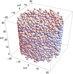
Figure 5: The simulated Lennard-Jones fluid consisted of 22091 particles moving in a closed cylindrical pillbox of radius $R=16.45\sigma$ and height $L=16.45\sigma$.

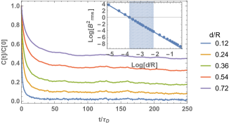
Figure 6: Magnetic field correlation function $C(t)$ at the NV’s position resulting from the dynamics of LJ particles confined to a cylinder. The field is evaluated at several values of NV implantation depth $d/R$. The dimensions of the cylinder were $R=L=16.45$. The particle density was $\rho=0.79\sigma^{-3}$. LJ fluid parameters in the reduced units were $\epsilon=1$, $\sigma=1$ and temperature $T=1$. The dynamics were integrated for $4\times 10^{6}$ timesteps of size $0.005\sqrt{\epsilon/(m\sigma^{2})}$. The correlation length was obtained by computing the power spectrum $S(\omega)=\left\langle|\mathscr{F}[B(t)]|^{2}\right\rangle$ and then performing the inverse Fourier transformation. The averaging was over 16 simulation runs. The correlation function at $t=0$ is presented at the inset. The colored region fits a linear line with a slope of $-2.7$. This scaling is similar to the $d^{-3}$ scaling predicted by Eq. (11) at small values of $d/R$.

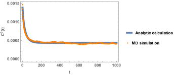
Figure 7: The magnetic field correlation function in a cylindrical geometry with $R=L=16.44\sigma$ and $d=8\sigma$. The correlation is given in arbitrary units, whereas the time is given in LJ units. The analytic curve was estimated by numerically calculating the first terms of Eq. (13) ($k,s\in[1,25]$) and adding the asymptotic constant given by Eq. (12). The simulation agrees with the analytic results apart from the value at $t=0$. This is because the limited integration time of the simulation is insufficient for estimating the power spectrum at $\omega=0$, which translates to an error in the estimation of $B_{rms}$.

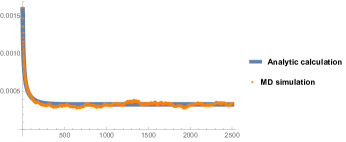
Figure 8: The magnetic field correlation function in a spherical geometry with $R=L=20.47\sigma$ and $d=8\sigma$. The correlation is given in arbitrary units, whereas the time is given in LJ units. The analytic curve was estimated by numerically calculating the first terms of Eq. (19) ($l\in[0,30],k\in[1,30]$) and adding the asymptotic constant given by Eq. (18). The simulation agrees well with the analytic results.

II.5 Limits of the model

In the calculation of the correlation function we performed an average over realizations of the magnetic field noise. While this averaging holds for correlation spectroscopy, in a phase sensitive measurement which is based on a single realization it does not. The main difference is that in a single realization, the statistical polarization will cause the amplitude of the signal to fluctuate as different nuclei diffuse in and out of the effective interaction region. Assuming the phase of the signal remains constant, the FI is bounded by that of the average amplitude, which is given by the correlation function. As long as the spins retain their initial polarization, the phase will remain stable. The spin orientation will eventually fluctuate, mostly due to the interaction between the nuclei and walls. The total measurement time $T$ in (28) is therefore limited by the characteristic time of the interaction, $T_{walls}$.

III CONCLUSION

We provided a theoretical basis for confined nano-NMR spectroscopy based on NV centers. We showed that the confinement indeed mitigates the deleterious effects of diffusion and therefore can be used to enhance the resolution abilities of both correlation spectroscopy and phase sensitive measurements. As advances are made with hyperpolarizationBucher et al. (2018); Shagieva et al. (2018b); Fernández-Acebal et al. (2018); Broadway et al. (2018); Abrams et al. (2014); Scheuer et al. (2016); London et al. (2013), it might prove more beneficial to combine polarization and confinement. The relevant calculations can be found in Sup .

IV Acknowledgments

We thank Carlos Meriles for pointing out the possibility of confinement to us. A. R. acknowledges the support of ERC grant QRES, project No. 770929, grant agreement No 667192(Hyperdiamond) and the ASTERIQS collaborative project.

References

- Jensen et al. (2017) K. Jensen, P. Kehayias, and D. Budker, “Magnetometry with nitrogen-vacancy centers in diamond,” in High Sensitivity Magnetometers, edited by A. Grosz, M. Haji-Sheikh, and S. Mukhopadhyay (Springer, Cham, Berlin, Heidelberg, 2017).
- Doherty et al. (2013) M. W. Doherty, N. B.Manson, P. Delaney, F. Jelezko, J. Wrachtrup, and L. C. L. Hollenberg, Phys. Rep. 528, 1 (2013).
- DeVience et al. (2015) S. J. DeVience, L. M. Pham, I. Lovchinsky, A. O. Sushkov, N. Bar-Gill, C. Belthangady, F. Casola, M. Corbett, H. Zhang, M. Lukin, H. Park, A. Yacoby, and R. L. Walsworth, Nat. Nanotech 10, 129 (2015).
- Mamin et al. (2013) H. J. Mamin, M. Kim, M. H. Sherwood, C. T. Rettner, K. Ohno, D. D. Awschalom, and D. Rugar, SCIENCE 339 (2013), 10.1126/science.1231540.
- Shagieva et al. (2018a) F. Shagieva, S. Zaiser, P. Neumann, D. B. R. Dasari, R. Stöhr, A. Denisenko, R. Reuter, C. A. Meriles, and J. Wrachtrup, Nano Lett. 18, 3731 (2018a).
- Pfender et al. (2019) M. Pfender, P. Wang, H. Sumiya, S. Onoda, W. Yang, D. B. R. Dasari, P. Neumann, X.-Y. Pan, J. Isoya, R.-B. Liu, and J. Wrachtrup, Nat. Commun 10, 594 (2019).
- Aslam et al. (2017) N. Aslam, M. Pfender, P. Neumann, R. Reuter, A. Zappe, F. F. de Oliveira, A. Denisenko, H. Sumiya, S. Onoda, J. Isoya, and J. Wrachtrup, SCIENCE 357 (2017), 10.1126/science.aam8697.
- Glenn et al. (2018) D. R. Glenn, D. B. Bucher, J. Lee, M. D. Lukin, H. Park, and R. L. Walsworth, Nature 555, 351 (2018).
- Bucher et al. (2018) D. B. Bucher, D. R. Glenn, H. Park, M. D. Lukin, and R. L. Walsworth, “Hyperpolarization-enhanced nmr spectroscopy with femtomole sensitivity using quantum defects in diamond,” (2018).
- Cohen et al. (2019) D. Cohen, T. Gefen, L. Ortiz, and A. Retzker, “Achieving the ultimate precision limit in quantum nmr spectroscopy,” (2019).
- Cohen et al. (2020) D. Cohen, R. Nigmatullin, O. Kenneth, F. Jelezko, M. Khodas, and A. Retzker, Sci. Rep. 10, 5298 (2020).
- (12) A. Rotem, S. Oviedo-Casado, and A. Retzker, In preperation .
- Staudacher et al. (2015) T. Staudacher, N. Raatz, S. Pezzagna, J. Meijer, F. Reinhard, C. A. Meriles, and J. Wrachtrup, Nat. Commun. 6, 8527 (2015).
- Kong et al. (2015) X. Kong, A. Stark, J. Du, L. P. McGuinness, and F. Jelezko, Physical Review Applied 4, 024004 (2015).
- Laraoui et al. (2013) A. Laraoui, F. Dolde, C. Burk, F. Reinhard, J. Wrachtrup, and C. A. Meriles, Nature communications 4, 1 (2013).
- Rosskopf et al. (2017) T. Rosskopf, J. Zopes, J. M. Boss, and C. L. Degen, npj Quantum Inf. 3 (2017), 10.1038/s41534-017-0030-6.
- Zaiser et al. (2016) S. Zaiser, T. Rendler, I. Jakobi, T. Wolf, S.-Y. Lee, S. Wagner, V. Bergholm, T. Schulte-Herbrüggen, P. Neumann, and J. Wrachtrup, Nat. Commun. 7 (2016), 10.1038/ncomms12279.
- Schmitt et al. (2017) S. Schmitt, T. Gefen, F. M. Stürner, T. Unden, G. Wolff, C. Müller, J. Scheuer, B. Naydenov, M. Markham, S. Pezzagna, J. Meijer, I. Schwarz, M. Plenio, A. Retzker, L. P. McGuinness, and F. Jelezko, SCIENCE 356, 6340 (2017).
- Boss et al. (2017) J. Boss, K. Cujia, J. Zopes, and C. Degen, Science 356, 837 (2017).
- (20) “See supporting information,” .
- DeGroot and Schervish (2012) M. H. DeGroot and M. J. Schervish, Probability and statistics (Pearson Education, 2012).
- Shagieva et al. (2018b) F. Shagieva, S. Zaiser, P. Neumann, D. Dasari, R. St öhr, A. Denisenko, R. Reuter, C. Meriles, and J. Wrachtrup, Nano letters 18, 3731 (2018b).
- Fernández-Acebal et al. (2018) P. Fernández-Acebal, O. Rosolio, J. Scheuer, C. Müller, S. Müller, S. Schmitt, L. P. McGuinness, I. Schwarz, Q. Chen, A. Retzker, et al., Nano letters 18, 1882 (2018).
- Broadway et al. (2018) D. A. Broadway, J.-P. Tetienne, A. Stacey, J. D. Wood, D. A. Simpson, L. T. Hall, and L. C. Hollenberg, Nature communications 9, 1246 (2018).
- Abrams et al. (2014) D. Abrams, M. E. Trusheim, D. R. Englund, M. D. Shattuck, and C. A. Meriles, Nano letters 14, 2471 (2014).
- Scheuer et al. (2016) J. Scheuer, I. Schwartz, Q. Chen, D. Schulze-Sünninghausen, P. Carl, P. Höfer, A. Retzker, H. Sumiya, J. Isoya, B. Luy, et al., New Journal of Physics 18, 013040 (2016).
- London et al. (2013) P. London, J. Scheuer, J.-M. Cai, I. Schwarz, A. Retzker, M. B. Plenio, M. Katagiri, T. Teraji, S. Koizumi, J. Isoya, et al., Physical review letters 111, 067601 (2013).