Weakly invasive metrology: quantum advantage and physical implementations
Abstract
We consider the estimation of a Hamiltonian parameter of a set of highly photosensitive samples, which are damaged after a few photons are absorbed, for a total time . The samples are modelled as a two mode photonic system, where photons simultaneously acquire information on the unknown parameter and are absorbed at a fixed rate. We show that arbitrarily intense coherent states can obtain information at a rate that scales at most linearly with and , whereas quantum states with finite intensity can overcome this bound. We characterise the quantum advantage as a function of and , as well as its robustness to imperfections (non-ideal detectors, finite preparation and measurement rates for quantum photonic states). We discuss an implementation in cavity QED, where Fock states are both prepared and measured by coupling atomic ensembles to the cavities. We show that superradiance, arising due to a collective coupling between the cavities and the atoms, can be exploited for improving the speed and efficiency of the measurement.
1 Introduction
One exciting prospect of quantum technologies are more precise photonic measurements through the use of quantum correlations [1, 2, 3, 4, 5]. Given a fixed (average) photon number , a variety of quantum states surpasses the shot-noise limit imposed by coherent states, notably squeezed, NOON or twin Fock states [6, 7, 8]. One of the motivations to limit is that some photosensitive materials may be damaged when they absorb too many photons. However, in this case it may be more meaningful to constrain the number of photons absorbed by the sample , instead of . Examples of delicate samples include biological [9, 10, 11, 12, 13, 14, 15], molecular [16] and atomic systems [17, 18]. For the latter, the maximal that the sample can tolerate can be a few photons, as quantum states such as the GHZ state can be extremely susceptible to noise.
The number of absorbed photons is not only determined by the but also in general depends on the time that the sample is exposed to light and its intrinsic properties. Still, for interferometric measurements [18, 19, 12, 13], placing a constraint in becomes essentially equivalent to fixing the total number of photons. Instead, in this work we will consider frequency measurements in which photons are allowed to interact continuously with the sample. In this case, we will show that constraining instead of leads to qualitatively new results.
In frequency measurements, both the probe size (e.g. the number of photons ) and the total time are resources for quantum metrology [8, 20, 21, 22], and interesting interplays between both appear when the probe is subject to noise or decoherence [20, 21, 22, 23, 24, 25, 26, 27]. Optimal metrological protocols for a fixed and have been considered for atomic measurements [20, 21, 22, 23, 24, 25, 26, 27], non-linear photonic systems [28], many-body open quantum systems [29], and time-dependent Hamiltonians [30, 31, 32]. Such time-optimized protocols can lead to a supraclassical scaling with of the measurement precision for specific types of correlated or directional noise [23, 24, 33, 25, 34, 35, 36, 26, 27], and to a constant advantage for uncorrelated noise [20, 37, 38, 39, 40].
Here, we investigate frequency measurements in a two-mode photonic system, where one wishes to estimate the strength of a beamsplitter-like interaction. This a common task when characterizing the coupling strength in devices such as coupled cavity modes, nanophotonic lattices, superconducting resonators or micromechanical resonators. In contrast to previous works (see, for example, [28]), we shall not put the constraint on , but on the energy that the system can absorb (). This subtle difference turns out to have important consequences: quantum metrological protocols involving a small amount of photons and a finite amount of samples, can overcome classical strategies using coherent states of (potentially) arbitrary intensity and an arbitrarily large number of samples. We quantify the quantum advantage as a function of and , and also discuss robustness to imperfections (non-ideal detectors, finite preparation and measurement times).
In a second part of the article, we develop a proposal for realising such enhancements in state-of-the-art technologies using a cavity or circuit QED set-up [41, 42]. The key idea is to couple each cavity to an atomic ensemble, and engineer the dynamics to both prepare and measure Fock states in the cavity. The collective coupling between the atoms and the cavity leads to the well-known phenomenon of Dicke superradiance [43], which has received renewed attention in the last years due to the experimental progress in cavity QED [44, 45, 46, 47, 48] and waveguide QED set-ups [49, 50, 51]. On the theoretical side, superradiance has been exploited for several applications of quantum photonic technologies [3, 4, 5, 52], including preparation of photonic states [53, 54, 55, 56], quantum number-resolved measurements [57, 58, 59], and quantum metrology [60, 61]. Here, we explore similar applications in the context of cavity or circuit QED, and we argue that the collective coupling can be exploited to increase the efficiency and speed of both the measurement and preparation of Fock states.
2 Framework and physical setup
We model the “delicate sample” as a two-mode photonic system, with and . We wish to estimate the interaction strength between modes ( has units of frequency and we set ). The inference process is mediated by photons, which can also be absorbed by the sample leading to its degradation. The latter process is modelled as a Markovian dissipative process, so that the time evolution of the photonic state reads:
| (1) |
with . With time, information on is encoded in , but also photons are lost (absorbed). These two dynamical processes decouple, so that the evolution can be described as two independent channels: , with and .
If the initial state contains photons, the (average) number of absorbed photons is given by
| (2) |
where counts the total number of photons. We shall assume that the delicate sample is destroyed when , which sets a maximum available time for information acquisition. This constrains the possible estimation schemes and, to some extent, can be seen as a resource: a larger enables us to obtain more information (and/or in a faster manner) from a single sample.
In order to estimate , we consider the following scenario: We have at our disposal a large number of delicate samples that we can measure sequentially for a total time . The same estimation scheme, or test, is applied to each sample. In each test, a photonic state is prepared, it evolves for some time according to (1) reaching , and is measured by an observable , which yields the outcome with probability . The whole experiment consists of tests, with each test taking a time , which must satisfy . Then, the uncertainty of an unbiased estimator of satisfies [62, 63, 64]:
| (3) |
Here, is the Classical Fisher Information (CFI) and is the quantum Fisher Information (QFI), which will be defined later for each case of interest, and characterizes the potential of for estimating with an optimal measurement [64]. Our goal is to minimize (3) for both coherent and quantum (e.g. Fock, NOON, or squeezed) states. In both cases, we set the two constraints:
-
•
the total time of the experiment.
-
•
the maximal number of photons that a single sample can absorb.
For coherent states, we shall put no more constraints, so that the photon number and the number of samples can be made arbitrarily large, which contrasts with previous works, see e.g. [21]. On the other hand, for quantum states, in Sec. 5 we will also constrain and the measurement efficiency, and consider a finite rate of preparation and measurement of quantum states.
It is worth pointing out that, defining , we can rewrite as , so an alternative interpretation of this framework is that we are estimating the frequency difference between two modes. In terms of the original modes and , both pictures are physically equivalent if a balanced beamsplitter is applied to the input (and output) light. With this transformation, it is also clear that the problem at hand can be formally mapped to standard Mach-Zehnder interferometry with , where photon absorption corresponds to a symmetric (time-dependent) photon loss. This map naturally enables us to use techniques and results developed in this context [1, 2, 3].
3 Optimal classical strategy
Let us first analyze the optimal strategy using coherent states. We consider as an input state with . The dissipative channel acts upon the initial state as . Since the state remains pure, we can quantify the QFI of as [64], obtaining:
| (4) |
which is the shot-noise-limit. Using and , the accumulated QFI in a time reads: This expression increases monotonically with , so its maximum is obtained for :
| (5) |
Strictly speaking, this bound can be saturated by testing samples, each for an infinitesimally small time using a number of photons, in such a way that both and remain constant. We call this theoretical limit ( and , with both and fixed) the Poisson limit, which will play a relevant role in this work. The importance of the classical bound (5) is that it remains finite –being limited by both and – despite using an unbounded photon number (at each test) and an arbitrarily large number of tests. We also note that optimality of fast measurements has also been found in frequency measurements of atomic ensembles [20, 23, 24, 25, 26, 27].
4 Quantum strategies
We now move to quantum resources. We begin by deriving an upper bound on given arbitrary quantum states. We use the results of Refs [65, 66, 37, 38, 39], where the upper bound is obtained for an optical interferometer with symmetric photon loss in both arms, as quantified by (the probability of photon loss in each arm of the interferometer). In the context studied here this translates as:
| (6) |
with and . In analogy with the classical derivation, an upper bound on the accumulated QFI for a given and can now be easily obtained using :
| (7) |
This expression also increases monotonically with , and for it simplifies to:
| (8) |
Approximating as for , we can express (8) in terms of as:
| (9) |
Comparing (9) with (5), we note that in principle an arbitrarily large advantage over the classical bound can be obtained in the Poisson limit (where and with and constant). For finite but large , the quantum advantage scales as . To understand intuitively this large advantage, we note that for states featuring Heisenberg scaling, which remains constant in the Poisson limit111In the Poisson limit, Heisenberg scaling may be preserved as when . This observation is not in contradiction with the well-known fact that quantum states lose Heisenberg scaling as for constant [65, 66, 37, 38, 39], as in this case remains finite as . These heuristic considerations will be made more precise for specific states in what follows. .
While the previous observations illustrate that large quantum advantages are possible in the Poisson limit, two very relevant questions appear: (i) how close specific quantum states can get to the upper bound Eq (8), and, more importantly: (ii) whether the classical bound (5) can be overcome in realistic scenarios where is small and imperfections are present (non-ideal measurements, finite time of preparation of quantum states). In what follows, we address (i) by computing for relevant quantum states in the Poisson limit. Question (ii) will be addressed in Sec. 5.
We start by the paradigmatic case of twin-Fock states (TFS) [7, 67, 68]. In this case, we have with and . This state evolves for a time according to (1), which we recall can be split in two independent channels: a unitary one which encodes , and a dissipative one where photons are lost with probability . The state after a time can then be described as:
| (10) |
where , and is the probability of absorving photons after a time , which is given by: . To compute the QFI of this state, it is convenient to note that given , with and ; the QFI reads with and [64, 69]. For TFS, we hence obtain,
| (11) |
Now, taking the Poisson limit of (11) ( with ), yields
| (12) |
with
| (13) |
For , the Poisson distribution (13) is strongly peaked around , such that the sum in (12) is dominated by . In this regime, , which is half of the upper bound (8). In contrast, as , . In general, a global measurement on both modes is needed to saturate the QFI (12) [69]. The has been considered for more realistic photon number-resolved measurements (NRM) [70, 68, 71, 72], and we study it in the Poisson limit in Sec. B of the Appendix. For , we find . The exponential decay with can be avoided by suitably optimising over the interaction strength , leading to a quasi-linear growth of with (see Fig. 1).
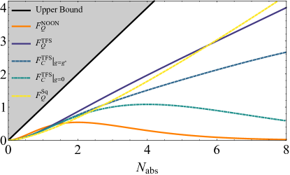
We now consider NOON states. In particular, we take as an initial state with . In this case, is given by times the probability of not losing any photon which, in the Poisson limit, is given by in (13). Hence,
| (14) |
For , NOON perform twice as good as TFS, but this advantage is exponentially suppressed for larger . In fact, NOON states are optimal for , which means that the bound (8) can not be saturated in this regime. In the regime , the upper bound (8) can be saturated using two mode squeezed states and number-resolved measurements [73, 74], which we show in Sec. A of the Appendix. The performance of TFS, squeezed and NOON states in the Poisson limit is summarised in Fig. 1. In the regime , the performance can be improved by considering more general states, such as the optimal states discussed in [75, 76, 77, 78, 66, 79, 80, 81].
Summarising, quantum photonic states (TFS, squeezed or NOON states) can provide an arbitrarily large advantage over the classical bound (5) in the Poisson limit, which however requires and (i.e. arbitrarily fast measurements). In the next section, we explore quantum advantages in realistic scenarios with small and finite , and also consider the presence of non-idealities in the preparation and measurement steps.
5 Quantum advantage in realistic scenarios
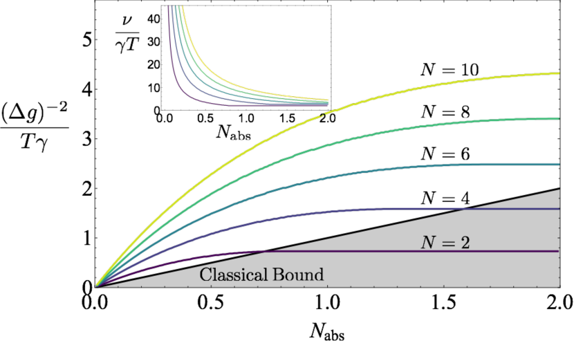
We first explore the presence of finite . First, when is finite with , we can use and to approximate as
| (15) |
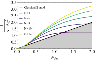
where is any of the CFI or QFI shown in Fig. 1. This expression can be compared with (5), where we note a linear increase of the quantum advantage with . Interestingly, quantum advantages are also observed when is small, so that Eq. (15) is not necessarily valid. This is shown in Fig. 2, where we compute the QFI of TFS exactly using (11) for low . Notably, we see that even quantum states with can outperform arbitrary classical strategies for sufficiently small . Importantly, the number of repetitions of the experiment is also small in such scenarios (see inset of Fig. 2 ). While these considerations are promising, the results of Fig. 2 are obtained assuming perfect preparation and measurement devices, which motivates the analysis of noise robustness in what follows.
Let us consider the main practical limitations: measurement devices with efficiency , and an extra time to prepare and measure quantum states [22]. More precisely, we model photon loss in the measurement process through a beamsplitter interaction with vacuum of each mode , :
| (16) |
so that there is a probability of losing a photon. Since is the same in both modes, this beam splitter interaction commutes with , so that this operation can be applied either before (imperfect state preparation) or after (imperfect detector) the acquisition of information of . In particular, we can generalise as: , where is independent of the time of the process, and where we recall that (i.e. the photons loss in the vacuum do not damage the sample). Indeed, quantifies the efficiency of the detector. On the other hand, we also assume the existence of an extra time to prepare and measure quantum states of light. The total time of the process is hence generalised to:
| (17) |
where is the time used in the interference process.
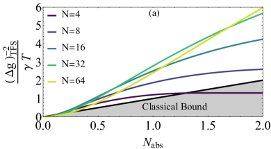
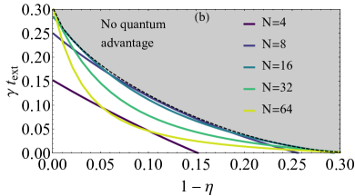
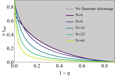
Given this model, we first illustrate in Fig. 3 (a) that TFS with low can overcome the bound (5) when is small, even in the presence of imperfections (in the figure, we take and ). These results can be compared with the ideal scenario ( and ) shown in Fig. 2, which illustrates that imperfections become most relevant as increases. Similar results are found for NRM (see Sec. C of the Appendix). Importantly, in both cases the corresponding protocol requires measuring a finite number of samples, , making it feasible in practice.
Second, the robustness of such quantum advantages to finite detector efficiency () and extra times () is analysed in Fig. 3 (b) for TFS and . In particular, we plot the values of for which for different . That is, on the left of the curves of Fig. 3 (b), quantum advantages are possible (i.e., ), and on the right, they are not. In the grey region, no quantum advantages are possible regardless of . Whereas for or increasing is generally favourable, we find that TFS of low () are most robust to noise when both and are non-negligible. In particular, for TFS of , the quantum advantage prevails for and .
In Sec. C of the Appendix, we provide an extended discussion of noise robustness, including upper bounds on general states. We find that, while the presence of and severely restricts the maximal possible quantum advantage, the main practical conclusion of our paper remains: In frequency measurements of delicate samples, few-photon quantum states (TFS, NOON, or squeezed) can overcome classical strategies using arbitrarily intense coherent states and an arbitrarily large number of samples when is low.
6 Implementation in Cavity QED
Although quantum advantages can be obtained already for low and can tolerate imperfections (see Fig. 3 and Sec. C of the Appendix), it is crucial to devise implementations where quantum states are prepared and measured fast, and with high efficiency. Recent examples include the preparation of Fock states in the motional states of trapped ions [82]. Here, we take an alternative route and outline a protocol based on cavity QED [41] or circuit QED [42] capable of generating and observing Fock states of light in cavities, inspired by recent progress on metrology and number-resolved measurements in waveguide QED [53, 83, 61, 59]. The key idea is to engineer an interaction of the cavity with a set of resonant qubits/atoms. More precisely, in addition to Eq. (1), the two cavities are each coupled to a collection of resonant atoms via
| (18) |
such that the total Hamiltonian of the system reads . In our protocol we require that the collectively enhanced atom–cavity coupling is tuneable and much faster than the cavity decay rate. Strong coupling, together with control of the atom–cavity interaction is routinely achieved in experiment [84, 48], in particular to generate or absorb individual photons [85]. Extending this level of control to ensembles of atoms the cavity and combining this with sufficiently high quality readout is challenging, but actively investigated [44, 86].
Initially, all atoms are excited, and each cavity is set to the ground state: , where is the number photons in each cavity. Through the atom-cavity (AC) Dicke interaction (18), the excitations are transformed into photons in the cavity. In general, we can diagonalize exactly Eq. (18) to find the state evolution (see Appendix D). Yet, here we provide an analytical solution in the linear regime where along the evolution, which turns out to also be relevant for the implementation. In this case, we can linearize the spin operator around the state with all atoms excited, obtaining , where is a bosonic annihilation operator. Thus, Eq. (18) transforms into
| (19) |
The time evolution is therefore a two-mode squeezing operation , with . Under this evolution,
| (20) | ||||
with . In particular, the optimal time scale to obtain on average photons in each cavity is
| (21) |
On the other hand, the probability of obtaining photons in one cavity at time is given by: . For the time (21), it reads:
| (22) |
which we recall holds in the regime .
Given these considerations, for a given target photon number , the state preparation protocol consists of the following steps.
-
1.
Starting from an initial state of all atoms and both cavities in the ground state, all atoms are excited.
-
2.
The cavity-atom interaction is turned on, , for a time .
-
3.
The cavity-atom interaction is turned off and the number of remaining excited atoms is measured.
Conditional on the measurement outcome , the cavity is projected in a Fock state with photons, which takes place with probability given in Eq. (22). This process can be done in parallel for both cavities, and on average photons are created.
After this preparation stage, we let the photonic system evolve according to Eq. (1) for some time , which is the time relevant for our discussion in the rest of the article. The number of photons involved in the process is . In the mean time, the remaining atoms need to be reset to the ground state in order to prepare them for the final measurement.
To measure the final photon distribution in the cavity, we again turn on the atom-cavity coupling , which allows the atoms to reabsorb photons from the cavity. In contrast to the preparation stage, the atoms are now prepared in the ground state, whereas the photonic state contains at most photons. As in the preparation stage, we can linearize the spin operator (now around the ground state) obtaining , where is a bosonic annihilation operator. Thus, Eq. (18) can now be transformed as
| (23) |
The time evolution is therefore a standard beam splitter interaction with oscillations with period . We take , i.e.
| (24) |
to maximise the probability that all photons are absorbed. Given a -photon state in the cavity as an initial state, this absorption process has an error probability , where is the probability that all photons are absorbed. In order to relate it to the efficiency of the detector, we can identify:
| (25) |
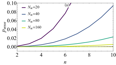
Note that, strictly speaking, the introduced here is not the same as the one introduced in (5) (in the sense that they arise through different physical processes), but their meaning is essentially the same: the probability of not losing a photon in the detection process. In particular, a small guarantees , as desired. The error probability is shown in Fig. 4 for different . From the figure, it becomes clear that for already very high efficiencies can be obtained, so that quantum advantages are possible according to Fig. 3. Furthermore, we note that, if is non-negligible, the absorption process can be repeated, which substantially reduces , as also shown in Fig. 4. In this case, adding up the total number of excitations observed in the measurements yields the measurement result, thus implementing a number-resolved measurement (NRM) in each cavity.
In practice, the following constraints need to be satisfied for the successful implementation of this scheme:
-
1.
, i.e., a high detector efficiency in the NRM, and
-
2.
, so that can be neglected.
The linear regime where is hence convenient for the implementation of this protocol, and it is also useful to engineer a strong atom-cavity coupling . Experimental requirements needed for the successful implementation of this proposal are discussed in the Sec. D of the Appendix, where we argue that both cavity QED [87, 88, 44] and circuit QED [89, 90, 91] appear as promising platforms.
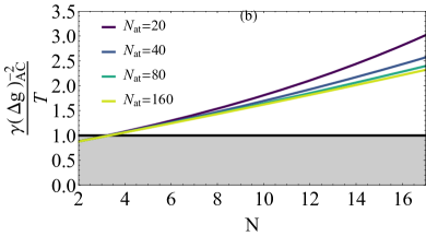
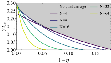
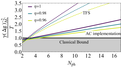
Even when both conditions are met, the discussed preparation scheme does not produce TFS, but rather Fock states distributed according to . Furthermore, the NRM in each cavity is in general not optimal for metrology, i.e., the corresponding CFI does not saturate (see Fig. 1, Appendix B, and Refs. [70, 71, 72]). While both effects lead to a reduction for the quantum advantages reported in Fig. 3, we find that quantum advantages can be obtained for , and with the discussed implementation, as shown in Fig. 4 for . Details on the calculation of for the atom-cavity (AC) implementation, as well as an analysis to robustness to non-idealities ( and ), is provided in Appendix D.
7 Conclusions
While quantum advantages in photonic metrology are well established when the (average) photon number is fixed [3, 4, 5], in specific situations, other constraints might be more meaningful. For example, when non-linear effects or quantum backaction limit the light intensity, a more sophisticated analysis has to take these effects into account [92]. Here, we study a complimentary situation, where photosensitive samples imply that the number of absorbed photons is limited [18, 12, 13, 14, 15]. While in interferometric measurements this coincides with the traditional constraint on , we have shown that it leads to qualitatively new results in frequency measurements. In this case, finite quantum resources for metrology (finite photon number, finite number of samples, finite time) can become more powerful than infinite classical resources (unbounded photon number, unlimited number of samples, finite time). We have characterized these advantages as a function of and for a model of two coupled oscillators, but our results suggest similar advantages in frequency measurements of delicate samples where photon absorption can be modelled as a Markovian process.
In a second part of the article, we have discussed a possible implementation of these advantages in a cavity QED set-up. The key idea is to couple cavities to a set of resonant atoms. By suitably controlling the atoms, we have devised strategies to prepare and measure Fock states in a fast and efficient way. In particular, we showed that superradiance, arising due to the collective atom-cavity coupling, can be exploited to enhance the quality of the measurement and preparation of photonic states. These results illustrate the potential of superradiance for applications in quantum metrology and information [52, 3, 4, 5].
Acknowledgements. We thank J. Kołodyński and M. W. Mitchell for insightful discussions. M. P.-L. acknowledges funding from Swiss National Science Foundation (Ambizione PZ00P2-186067). D.M. and J.I.C. acknowledge funding from ERC Advanced Grant QENOCOBA under the EU Horizon 2020 program (Grant Agreement No. 742102).
References
- Giovannetti et al. [2011] V. Giovannetti, S. Lloyd, and L. Maccone, Nature Photonics 5, 222 (2011).
- Tóth and Apellaniz [2014] G. Tóth and I. Apellaniz, Journal of Physics A: Mathematical and Theoretical 47, 424006 (2014).
- Demkowicz-Dobrzański et al. [2015] R. Demkowicz-Dobrzański, M. Jarzyna, and J. Kołodyński, in Progress in Optics (Elsevier, 2015) pp. 345–435.
- Dowling and Seshadreesan [2015] J. P. Dowling and K. P. Seshadreesan, Journal of Lightwave Technology 33, 2359 (2015).
- Polino et al. [2020] E. Polino, M. Valeri, N. Spagnolo, and F. Sciarrino, AVS Quantum Science 2, 024703 (2020).
- Caves [1981] C. M. Caves, Phys. Rev. D 23, 1693 (1981).
- Holland and Burnett [1993] M. J. Holland and K. Burnett, Phys. Rev. Lett. 71, 1355 (1993).
- Bollinger et al. [1996] J. J. . Bollinger, W. M. Itano, D. J. Wineland, and D. J. Heinzen, Phys. Rev. A 54, R4649 (1996).
- Neuman et al. [1999] K. C. Neuman, E. H. Chadd, G. F. Liou, K. Bergman, and S. M. Block, Biophysical Journal 77, 2856 (1999).
- Peterman et al. [2003] E. J. Peterman, F. Gittes, and C. F. Schmidt, Biophysical Journal 84, 1308 (2003).
- Cole [2014] R. Cole, Cell Adhesion & Migration 8, 452 (2014).
- Taylor et al. [2013] M. A. Taylor, J. Janousek, V. Daria, J. Knittel, B. Hage, H.-A. Bachor, and W. P. Bowen, Nature Photonics 7, 229 (2013).
- Taylor et al. [2014] M. A. Taylor, J. Janousek, V. Daria, J. Knittel, B. Hage, H.-A. Bachor, and W. P. Bowen, Phys. Rev. X 4, 011017 (2014).
- Taylor and Bowen [2016] M. A. Taylor and W. P. Bowen, Physics Reports 615, 1 (2016).
- Whittaker et al. [2017] R. Whittaker, C. Erven, A. Neville, M. Berry, J. L. O’Brien, H. Cable, and J. C. F. Matthews, New Journal of Physics 19, 023013 (2017).
- Pototschnig et al. [2011] M. Pototschnig, Y. Chassagneux, J. Hwang, G. Zumofen, A. Renn, and V. Sandoghdar, Phys. Rev. Lett. 107, 063001 (2011).
- Eckert et al. [2007] K. Eckert, O. Romero-Isart, M. Rodriguez, M. Lewenstein, E. S. Polzik, and A. Sanpera, Nature Physics 4, 50 (2007).
- Wolfgramm et al. [2012] F. Wolfgramm, C. Vitelli, F. A. Beduini, N. Godbout, and M. W. Mitchell, Nature Photonics 7, 28 (2012).
- Ono et al. [2013] T. Ono, R. Okamoto, and S. Takeuchi, Nature Communications 4 (2013), 10.1038/ncomms3426.
- Huelga et al. [1997] S. F. Huelga, C. Macchiavello, T. Pellizzari, A. K. Ekert, M. B. Plenio, and J. I. Cirac, Phys. Rev. Lett. 79, 3865 (1997).
- Shaji and Caves [2007] A. Shaji and C. M. Caves, Phys. Rev. A 76, 032111 (2007).
- Hayes et al. [2018] A. J. Hayes, S. Dooley, W. J. Munro, K. Nemoto, and J. Dunningham, Quantum Science and Technology 3, 035007 (2018).
- Matsuzaki et al. [2011] Y. Matsuzaki, S. C. Benjamin, and J. Fitzsimons, Phys. Rev. A 84, 012103 (2011).
- Chin et al. [2012] A. W. Chin, S. F. Huelga, and M. B. Plenio, Phys. Rev. Lett. 109, 233601 (2012).
- Chaves et al. [2013] R. Chaves, J. B. Brask, M. Markiewicz, J. Kołodyński, and A. Acín, Phys. Rev. Lett. 111, 120401 (2013).
- Brask et al. [2015] J. B. Brask, R. Chaves, and J. Kołodyński, Phys. Rev. X 5, 031010 (2015).
- Smirne et al. [2016] A. Smirne, J. Kołodyński, S. F. Huelga, and R. Demkowicz-Dobrzański, Phys. Rev. Lett. 116, 120801 (2016).
- Woolley et al. [2008] M. J. Woolley, G. J. Milburn, and C. M. Caves, New Journal of Physics 10, 125018 (2008).
- Beau and del Campo [2017] M. Beau and A. del Campo, Phys. Rev. Lett. 119, 010403 (2017).
- Naghiloo et al. [2017] M. Naghiloo, A. N. Jordan, and K. W. Murch, Phys. Rev. Lett. 119, 180801 (2017).
- Pang and Jordan [2017] S. Pang and A. N. Jordan, Nature Communications 8 (2017), 10.1038/ncomms14695.
- Sun et al. [2020] L. Sun, X. He, C. You, C. Lv, B. Li, S. Lloyd, and X. Wang, arXiv preprint arXiv:2004.01216 (2020).
- Dorner [2012] U. Dorner, New Journal of Physics 14, 043011 (2012).
- Dür et al. [2014] W. Dür, M. Skotiniotis, F. Fröwis, and B. Kraus, Phys. Rev. Lett. 112, 080801 (2014).
- Kessler et al. [2014] E. M. Kessler, I. Lovchinsky, A. O. Sushkov, and M. D. Lukin, Phys. Rev. Lett. 112, 150802 (2014).
- Arrad et al. [2014] G. Arrad, Y. Vinkler, D. Aharonov, and A. Retzker, Phys. Rev. Lett. 112, 150801 (2014).
- Escher et al. [2011] B. Escher, R. de Matos Filho, and L. Davidovich, Nature Physics 7, 406 (2011).
- Demkowicz-Dobrzański et al. [2012] R. Demkowicz-Dobrzański, J. Kołodyński, and M. Guţă, Nature Communications 3 (2012), 10.1038/ncomms2067.
- Kołodyński and Demkowicz-Dobrzański [2013] J. Kołodyński and R. Demkowicz-Dobrzański, New Journal of Physics 15, 073043 (2013).
- Knysh et al. [2014] S. I. Knysh, E. H. Chen, and G. A. Durkin, arXiv preprint arXiv:1402.0495 (2014).
- Haroche and Raimond [2006] S. Haroche and J.-M. Raimond, Exploring the Quantum, Vol. 5 (Oxford University Press, 2006) p. 11.
- Blais et al. [2020] A. Blais, S. M. Girvin, and W. D. Oliver, Nature Physics 16, 247 (2020).
- Dicke [1954] R. H. Dicke, Phys. Rev. 93, 99 (1954).
- Haas et al. [2014] F. Haas, J. Volz, R. Gehr, J. Reichel, and J. Esteve, Science 344, 180 (2014).
- Norcia et al. [2016] M. A. Norcia, M. N. Winchester, J. R. K. Cline, and J. K. Thompson, Science Advances 2, e1601231 (2016).
- Hosseini et al. [2017] M. Hosseini, Y. Duan, K. M. Beck, Y.-T. Chen, and V. Vuletić, Phys. Rev. Lett. 118, 183601 (2017).
- Kim et al. [2018] J. Kim, D. Yang, S.-h. Oh, and K. An, Science 359, 662 (2018).
- Frisk Kockum et al. [2019] A. Frisk Kockum, A. Miranowicz, S. De Liberato, S. Savasta, and F. Nori, Nature Reviews Physics 1, 19 (2019), arXiv:1807.11636 .
- Mlynek et al. [2014] J. A. Mlynek, A. A. Abdumalikov, C. Eichler, and A. Wallraff, Nat. Commun. 5, 5186 (2014).
- Goban et al. [2015] A. Goban, C.-L. Hung, J. Hood, S.-P. Yu, J. Muniz, O. Painter, and H. Kimble, Phys. Rev. Lett. 115, 063601 (2015).
- Solano et al. [2017] P. Solano, P. Barberis-Blostein, F. K. Fatemi, L. A. Orozco, and S. L. Rolston, Nature Communications 8, 1857 (2017).
- O'Brien et al. [2009] J. L. O'Brien, A. Furusawa, and J. Vučković, Nature Photonics 3, 687 (2009).
- González-Tudela et al. [2017] A. González-Tudela, V. Paulisch, H. J. Kimble, and J. I. Cirac, Phys. Rev. Lett. 118, 213601 (2017).
- Paulisch et al. [2018] V. Paulisch, H. J. Kimble, J. I. Cirac, and A. González-Tudela, Phys. Rev. A 97, 053831 (2018).
- Uria et al. [2020] M. Uria, P. Solano, and C. Hermann-Avigliano, Phys. Rev. Lett. 125, 093603 (2020).
- Groiseau et al. [2020] C. Groiseau, A. E. Elliott, S. J. Masson, and S. Parkins, arXiv preprint arXiv:2012.00246 (2020).
- Romero et al. [2009] G. Romero, J. J. García-Ripoll, and E. Solano, Physical Review Letters 102, 173602 (2009).
- Peropadre et al. [2011] B. Peropadre, G. Romero, G. Johansson, C. M. Wilson, E. Solano, and J. J. García-Ripoll, Physical Review A 84, 063834 (2011).
- Malz and Cirac [2020] D. Malz and J. I. Cirac, Phys. Rev. Research 2, 033091 (2020).
- Paulisch et al. [2019a] V. Paulisch, M. Perarnau-Llobet, A. González-Tudela, and J. I. Cirac, Physical Review A 99, 043807 (2019a).
- Perarnau-Llobet et al. [2020] M. Perarnau-Llobet, A. González-Tudela, and J. I. Cirac, Quantum Science and Technology 5, 025003 (2020).
- Helstrom [1976] C. W. Helstrom, Quantum Detection and Estimation Theory (Elsevier Science, 1976).
- Holevo [1982] A. S. Holevo, Probabilistic and Statistical Aspects of Quantum Theory (Statistics & Probability) (English and Russian Edition) (Elsevier Science, 1982).
- Braunstein and Caves [1994] S. L. Braunstein and C. M. Caves, Phys. Rev. Lett. 72, 3439 (1994).
- Fujiwara and Imai [2008] A. Fujiwara and H. Imai, Journal of Physics A: Mathematical and Theoretical 41, 255304 (2008).
- Knysh et al. [2011] S. Knysh, V. N. Smelyanskiy, and G. A. Durkin, Phys. Rev. A 83, 021804 (2011).
- Campos et al. [2003] R. A. Campos, C. C. Gerry, and A. Benmoussa, Phys. Rev. A 68, 023810 (2003).
- Datta et al. [2011] A. Datta, L. Zhang, N. Thomas-Peter, U. Dorner, B. J. Smith, and I. A. Walmsley, Phys. Rev. A 83, 063836 (2011).
- Paris [2009] M. G. A. Paris, International Journal of Quantum Information 07, 125 (2009).
- Kim et al. [1998] T. Kim, O. Pfister, M. J. Holland, J. Noh, and J. L. Hall, Phys. Rev. A 57, 4004 (1998).
- Pezzé and Smerzi [2013] L. Pezzé and A. Smerzi, Phys. Rev. Lett. 110, 163604 (2013).
- Zhong et al. [2017] W. Zhong, Y. Huang, X. Wang, and S.-L. Zhu, Phys. Rev. A 95, 052304 (2017).
- Yurke et al. [1986] B. Yurke, S. L. McCall, and J. R. Klauder, Phys. Rev. A 33, 4033 (1986).
- Olivares and Paris [2007] S. Olivares and M. G. A. Paris, Optics and Spectroscopy 103, 231 (2007).
- Šafránek and Fuentes [2016] D. Šafránek and I. Fuentes, Phys. Rev. A 94, 062313 (2016).
- Huver et al. [2008] S. D. Huver, C. F. Wildfeuer, and J. P. Dowling, Phys. Rev. A 78, 063828 (2008).
- Dorner et al. [2009] U. Dorner, R. Demkowicz-Dobrzanski, B. J. Smith, J. S. Lundeen, W. Wasilewski, K. Banaszek, and I. A. Walmsley, Phys. Rev. Lett. 102, 040403 (2009).
- Demkowicz-Dobrzanski et al. [2009] R. Demkowicz-Dobrzanski, U. Dorner, B. J. Smith, J. S. Lundeen, W. Wasilewski, K. Banaszek, and I. A. Walmsley, Phys. Rev. A 80, 013825 (2009).
- Cable and Durkin [2010] H. Cable and G. A. Durkin, Phys. Rev. Lett. 105, 013603 (2010).
- Calsamiglia et al. [2016] J. Calsamiglia, B. Gendra, R. Muñoz-Tapia, and E. Bagan, New Journal of Physics 18, 103049 (2016).
- Matsubara et al. [2019] T. Matsubara, P. Facchi, V. Giovannetti, and K. Yuasa, New Journal of Physics 21, 033014 (2019).
- Wolf et al. [2019] F. Wolf, C. Shi, J. C. Heip, M. Gessner, L. Pezzè, A. Smerzi, M. Schulte, K. Hammerer, and P. O. Schmidt, Nature Communications 10 (2019), 10.1038/s41467-019-10576-4.
- Paulisch et al. [2019b] V. Paulisch, M. Perarnau-Llobet, A. González-Tudela, and J. I. Cirac, Phys. Rev. A 99, 043807 (2019b).
- Walther et al. [2006] H. Walther, B. T. H. Varcoe, B.-G. Englert, and T. Becker, Reports on Progress in Physics 69, 1325 (2006).
- Hennrich et al. [2000] M. Hennrich, T. Legero, A. Kuhn, and G. Rempe, Physical Review Letters 85, 4872 (2000).
- Mivehvar et al. [2021] F. Mivehvar, F. Piazza, T. Donner, and H. Ritsch, (2021), arXiv:2102.04473 .
- Zhang et al. [2012] H. Zhang, R. McConnell, S. Ćuk, Q. Lin, M. H. Schleier-Smith, I. D. Leroux, and V. Vuletić, Physical Review Letters 109, 133603 (2012).
- Hume et al. [2013] D. B. Hume, I. Stroescu, M. Joos, W. Muessel, H. Strobel, and M. K. Oberthaler, Physical Review Letters 111, 253001 (2013), arXiv:1307.7598 .
- Jeffrey et al. [2014] E. Jeffrey, D. Sank, J. Y. Mutus, T. C. White, J. Kelly, R. Barends, Y. Chen, Z. Chen, B. Chiaro, A. Dunsworth, A. Megrant, P. J. J. O’Malley, C. Neill, P. Roushan, A. Vainsencher, J. Wenner, A. N. Cleland, and J. M. Martinis, Physical Review Letters 112, 190504 (2014).
- Walter et al. [2017] T. Walter, P. Kurpiers, S. Gasparinetti, P. Magnard, A. Potočnik, Y. Salathé, M. Pechal, M. Mondal, M. Oppliger, C. Eichler, and A. Wallraff, Physical Review Applied 7, 054020 (2017).
- Dassonneville et al. [2020] R. Dassonneville, T. Ramos, V. Milchakov, L. Planat, Dumur, F. Foroughi, J. Puertas, S. Leger, K. Bharadwaj, J. Delaforce, C. Naud, W. Hasch-Guichard, J. J. García-Ripoll, N. Roch, and O. Buisson, Physical Review X 10, 11045 (2020).
- Mitchell [2017] M. W. Mitchell, Quantum Science and Technology 2, 044005 (2017).
- Thompson et al. [1992] R. J. Thompson, G. Rempe, and H. J. Kimble, Physical Review Letters 68, 1132 (1992).
- Brune et al. [1996] M. Brune, F. Schmidt-Kaler, A. Maali, J. Dreyer, E. Hagley, J. M. Raimond, and S. Haroche, Physical Review Letters 76, 1800 (1996).
- Yoshie et al. [2004] T. Yoshie, A. Scherer, J. Hendrickson, G. Khitrova, H. M. Gibbs, G. Rupper, C. Ell, O. B. Shchekin, and D. G. Deppe, Nature 432, 200 (2004).
- Wallraff et al. [2004] A. Wallraff, D. I. Schuster, A. Blais, L. Frunzio, R.-S. Huang, J. Majer, S. Kumar, S. M. Girvin, and R. J. Schoelkopf, Nature 431, 162 (2004).
- Reithmaier et al. [2004] J. P. Reithmaier, G. Sęk, A. Löffler, C. Hofmann, S. Kuhn, S. Reitzenstein, L. V. Keldysh, V. D. Kulakovskii, T. L. Reinecke, and A. Forchel, Nature 432, 197 (2004).
- Chiorescu et al. [2004] I. Chiorescu, P. Bertet, K. Semba, Y. Nakamura, C. J. P. M. Harmans, and J. E. Mooij, Nature 431, 159 (2004).
- Reiserer and Rempe [2015] A. Reiserer and G. Rempe, Reviews of Modern Physics 87, 1379 (2015).
Appendix A Squeezed states
Squeezed states also enable Heisenberg scaling [73, 74], and hence can provide a finite amount of information in the Poisson limit and . This is explored in this section.
We take as an initial state a vacuum-squeezed state together with a coherent-squeezed state: with , and , and ; and we take and . The average total number of photons is:
| (26) |
and it is convenient to define: , . We consider number-resolved measurements in the output states. Following [74], the in the regime is given by (the extra factor comes from the fact that we are measuring a frequency):
| (27) |
Taking the Poisson limit ( with ), leads to
| (28) |
At this point one can maximise this expression with respect to , with the constraints and , in order to optimise the measurement precision. For , we find that , hence squeezed states perform close to NOON states in this regime. On the other hand, for , we have , thus saturating the upper bound presented in the main text. For intermediate values of , a numerical optimisation is presented in Fig. 1 of the main text. It remains an interesting question whether more generalised Gaussian states and/or measurement schemes [75, 81] can outperform this proposal in this regime.
Appendix B Classical Fisher Information for number-resolved measurements
In this section we compute the classical Fisher information,
| (29) |
where is the probability to obtain outcome , for number resolved measurements in the set-up described in the main text. Because of the map between our framework and Mach-Zehnder interferometry with symmetric (time-dependent) photon loss, we can follow similar derivations in that context, see e.g. Refs. [70, 71, 72]. Let us first compute the probabilities of the photon-number measurements for the initial Fock state and unitary . First of all we note that commutes with the initial state (with a well defined photon number in each arm) and hence can be ignored for the number-resolved statistics. We first compute:
| (30) |
with and . Noting that:
| (31) |
we obtain
| (32) |
where we defined , and . This can also be expressed as:
| (33) |
where is the generalized hypergeometric function.
Next, we compute the probability to obtain outcomes for the state:
| (34) |
with
| (35) |
It is convenient to introduce:
| (36) |
Then, we have for (34)
| (37) |
The only remaining step is to compute the classical Fisher information using (29):
| (38) |
To gain some analytical insight for this expression, we can compute it in the limit . Following [71, 61], we can expand the probabilities around up to order , and realise that only instances where photons are measured in one of the modes contribute to the CFI. This leads to the following analytical expression for the CFI [68]:
| (39) |
which shows an exponential decay with . This is hence far from for large , while still better than NOON states. For future convenience, we also give the corresponding expression when the initial state is :
| (40) |
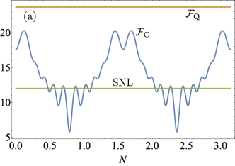
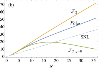
Finally, we numerically compute (38) for different , and for the state (34) (and setting ). An example is shown in Fig. 5, from it we see that in general the dependence of with is non-trivial, and so is the point where it is maximized. The figure also shows that indeed (29) does not saturate for number-resolved measurements. In Fig. 5 we also show (38) as a function of , where it becomes apparent the importance of maximizing with respect to for the number-resolved-measurements as increases. The numerical results suggest that a systematic improvement with respect to the Shot-Noise-Limit can be obtained for any with suitably optimized number-resolved-measurements.
Let us now look at the Poisson limit , while satisfying . First, from (39), we can study the Poisson limit , where we obtain:
| (41) |
To obtain similar analytical expression for arbitrary is challenging due to the complexity of obtaining asymptotic expressions for the generalized hypergeometric functions. Yet, we can obtain numerical results for rather large . To do this, it is useful to approximate in (38) as:
| (42) |
since only terms with and contribute to the sum in the Poisson limit (other terms are exponentially small). In our numerical simulations, we take and , and the results become in practice indistinguishable when these parameters are varied. Numerical results are shown in Fig. 2 of the main text.
B.0.1 Optimal measurement
Appendix C Robustness to imperfections: Photon loss in the detection process and finite time for preparation and measurement of quantum states
In this section, we discuss how of general quantum states decreases due to: finite , photon loss in the measurement process, and an extra-time of preparation/measurement of quantum resources. We then also discuss the particular case of twin Fock states (TFS), both with optimal measurements () and with photon number-resolved measurements (NRM) ().
We start by giving general bounds on for any quantum state given different constraints:
-
•
Finite N. Let us first assume finite , but and . Using the upper bound of [65, 66, 37, 38, 39], we have:
(44) where the factor comes from the fact that we are measuring a frequency-like quantity. Considering now measurements, we obtain:
(45) Since any or can only decrease , this bound also holds for any and .
-
•
Photon loss. Let us now assume . The starting point is now: , which implies for the whole process with measurements:
(46) which we expressed in terms of the constants and . The right hand side of (46) is maximised for (or equivalently ), leading to the bound:
(47) Hence the quantum advantage comes in the form of a better prefactor . This prefactor advantage takes the same form as the one obtained in noisy photon interferometry when comparing coherent and quantum states with a fixed [65, 66, 37, 38, 39].
-
•
Extra time. Let us now assume an extra time necessary to prepare and measure using quantum resources. Let us consider the extreme case but and no constraints on . Taking , we have:
(48) This expression is again optimised in the limit (and hence ), yielding:
(49)
Let us now consider the general case where and . In general we have,
| (50) |
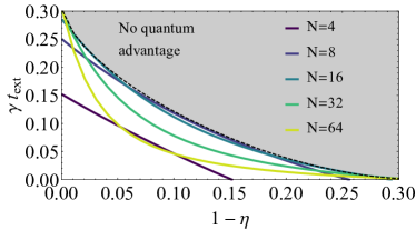
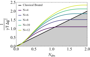
This expression is no longer optimised in general at , and in fact it does not allow for an analytical solution. We can still solve it numerically for any value of the desired value of , which provides an upper bound on the quantum advantage. In particular, a quantum advantage is impossible if . This condition is plot in Fig. 6, where we compute the values of for which . In Fig. 6, we also plot the values for which but by fixing implicitly by , which provide upper bounds for a state with photons. Interestingly, we find that the upper bound becomes more robust to noise in the regime where both and are not close to zero. This suggests that in realistic implementations few-photon quantum states are desirable when is low.
Let us now move to the particular case of TFS by considering and . It is useful to point out that, as long as ( needs to be determined in each case, e.g., numerically), (and ) is maximised by testing each sample until it is damaged, that is:
| (51) |
for (otherwise, the choice (51) is taken with ), and we recall that needs to be determined numerically for each case. Given this choice, we first analyse the regions where quantum advantages are possible using TFS, which is shown in Fig. 6. As expected, the regions are more restrictive than for the upper bound shown in Fig. 7. On the other hand, an example of the quantum advantage as a function of for different TFS and with and is presented in Fig. 8. Similar results are obtained when considering with NRM, which is in general lower than as expected from Fig. 5. This is shown in both Figs. 7 and 8 by considering .
Appendix D Measurement precision in cavity QED implementation
In this section we discuss the implementation in cavity QED, and in particular how to compute the measurement precision (both QFI and CFI).
At each run of the experiment, the preparation returns probabilistically a Fock state , where the photon numbers are known due to measurement of the remaining excited atoms, and are distributed according to the known distribution [Eq. (22)]. Given , the interaction time between cavities is taken such that on average photons are absorbed, i.e.:
| (52) |
We then repeat the experiment as often as possible in the given finite maximum time , such that in the end , where we defined which is the number of times a certain combination appeared in the experimental run. We are interested in the regime (i.e. ), where the statistics are dominated by typical sequences in which which, together with , provides .
Assuming a large number of runs of the experiment (so that enough statistics for each are obtained), the measurement uncertainty is bounded by
| (53) |
with is the QFI for an initial Fock state , and it reads (following the same reasoning provided in the main text):
| (54) | ||||
with and .
We can compute using NRM in a similar fashion. For simplicity, we focus on the case , which can be solved analytically, but the case of general can be straightforwardly treated following our previous considerations for TFS. Analogously with our previous considerations, we have,
| (55) |
with (see Eq. (40)),
| (56) |
with .
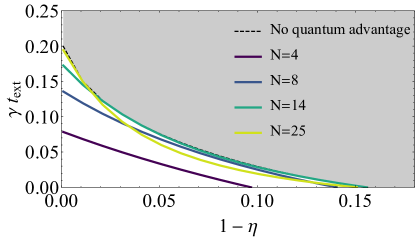
We show in Fig. 9, where it is compared with TFS. In our simulations, we compute exactly by solving the Hamiltonian Eq. (12) of the main text. As expected, the probabilistic preparation of Fock states in our implementation diminishes its performance with respect to ideal TFS. Yet, we see that already at , quantum advantages appear possible, even in the presence of detector inefficiencies (). The tolerance to imperfections (both and of is shown in Fig. 10.
D.0.1 Error sources in the cavity QED and circuit QED implementation
In practice, there are several additional sources of error in this protocol that ought to be considered.
First, we have assumed that all atoms/qubits are exactly on resonance with the cavity. Realistically, they may have differing energies and be detuned from the cavity, which makes the photon exchange between cavity and atoms less efficient. However, measuring the number of excited atoms after the interaction period still projects the cavity state onto a Fock state, such that disorder only affects the probability distribution of the produced Fock states, but not their fidelity.
Second, the fidelity of the generated Fock state is intrinsically limited by measurement error in the atomic readout. High-fidelity atom readout has already been demonstrated for large numbers of atoms in cavity QED [87, 88] and for intermediate numbers of qubits in circuit QED [89, 90, 91].
Third, the atoms need to be reset to ground state in a time much faster than . This is feasible if the cavity coupling is tunable (e.g., via an intermediate resonator in circuit QED) or if a fast decay channel is used (e.g., a fast optical transition of the atom).
Fourth, no photons may be lost throughout the experiment. This requires ultra-high finesse cavities or long qubit coherence times on the scale of , i.e., this requires the strong coupling regime, which has been achieved in both cavity and circuit QED [93, 94, 95, 96, 97, 98]. While the measurement is more challenging than the preparation, it relies on the same experimental figures of merit. A large advantage of our scheme is that one can post-select on successful runs of the experiment by requiring that at the end excitations are measured.
As an illustration, let us take the parameters from the experiment by Haas et al. [44]. These authors placed 40 atoms into a cavity of linewidth MHz with an atom–cavity coupling of MHz. Given a time , the probability that a photon leaks out of the cavity is hence , and the efficiency defined in (5) is given by . If we aim to prepare on average photons, Eq. (21) gives a preparation time of ns. The measurement time is given by (24), which for gives . Hence, we have for the overall process of preparation and measurement of 8 photons. On top of that, there is a probability that one of the photons stays in the cavity (c.f. Fig. 4), but from (25) we see this has a negligible effect on the total efficiency . Assuming that the atoms can be measured perfectly (current experiments show more than 99% measurement fidelity [87, 88]), this leads to an overall measurement efficiency of . This can be contrasted with Fig. 10, where we note that this experiment is on the verge of enabling quantum advantages in the proposed set-up. In order to increase the value of , a natural strategy is to reduce the linewidth of the cavity (increasing the number of atoms would also result in a larger , as discussed in the main text). In this sense, we should emphasize here that the experiment by Haas et al. does not include tuneable atom–cavity coupling and thus cannot directly be used to implement the scheme presented in the main text. To engineer a tuneable coupling, a Raman scheme has to be employed, and correspondingly much narrower cavities should be used [99], which will significantly enhance the preparation fidelity.
D.0.2 Non-linear regime and optimal time scale
As a final comment, we note that it is in principle possible to use this protocol in the non-linear regime . Indeed, it might be useful in particular experimental implementations to take most use of the atoms at hand. We hence here discuss a few properties of and in this regime.
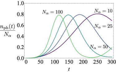
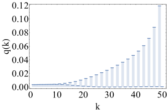
We start by investigating the average photon number in the cavity during the preparation stage. We see that reaches its maximum value at . The distribution for that optimal time is also illustrated in Fig. 11.
Let us now show that is well approximated by . Let us consider the Hamiltonian
| (57) |
where are the annihilation operators for two harmonic oscillators. corresponds to what formerly was a spin, and is just the same cavity mode as before. In the subspace spanned by the states , where are Fock states of an oscillator, the Hamiltonian is a bi-diagonal matrix
| (58) |
where
| (59) |
For large these are essentially the same matrix elements as the actual Hamiltonian (Eq. (12) in the main text) and one can check numerically that the dynamics is very similar for large enough . In the classical limit, we replace the annihilation operators by the amplitudes of the corresponding coherent states. The classical (mean field) equations of motion read
| (60) |
with initial conditions , .
Now we do a change of variables, taking , , such that
| (61a) | ||||
| (61b) | ||||
where . Further defining the constant , and the variable , we obtain the equations of motion
| (62a) | ||||
| (62b) | ||||
This defines a vector field in a two-dimensional plane, whose closed orbits are the possible trajectories of the system. Since the phase is ill-defined in the initial state, we can choose it to be . In this case, the system is governed only by
| (63) |
which is readily integrated to yield
| (64) |
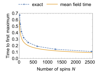
Since initially, and (taking and ), we conclude that the natural timescale for the switch is
| (65) |
This converges to the actual optimal time scale in the limit of large as we show in Fig. 12.
