Continuous limits of Heterogeneous Continuous Time Random Walk

Abstract

Continuous time random Walk model has been versatile analytical formalism for studying and modeling diffusion processes in heterogeneous structures, such as disordered or porous media. We are studying the continuous limits of Heterogeneous Continuous Time Random Walk model, when a random walk is making jumps on a graph within different time-length. We apply the concept of a generalized master equation to study heterogeneous continuous-time random walks on networks. Depending on the interpretations of the waiting time distributions the generalized master equation gives different forms of continuous equations.

I Introduction

The continuous time random walk (CTRW) model has been widely used for modelling dynamics inside porous media Scher1973 . However homogeneous random walk models do not exhaust the whole variety of dynamical phenomena Sahimi2012 ; Berkowitz2000 . The effects of heterogeneities on stochastic dynamics have been investigated in random trap and barrier models Thiel2016 ; Sokolov2010 . Recently there have been several studies, which describe models of random walks in heterogeneous medium. In particular, in Heterogeneous Continuous Time Random Walk (HCTRW) model on a network, introduced in GrebTupikina , a random walk is moving from one site $x$ to $x^{\prime}$ with the waiting time distribution $\psi_{xx^{\prime}}(t)$ depending on the link. HCTRW model allows one to introduce the local heterogeneity encoded through the distributions of travel times TuGrebenk , therefore it is of the general interest to develop a continuous equivalent of HCTRW model and explore its potential for description of diffusion models.

The fractional diffusion equations were recognized as a useful tool for the description of anomalous diffusion in disordered medium Chechkin2006 . In some cases corresponding fractional differential equations have been investigated Hughes ; Nigris . For homogeneous CTRW, when all waiting time distributions are fixed, the corresponding continuous dynamics is described by fractional diffusion equation with a Riemann-Liouville fractional derivative Barkai ; Schumer . However for cases when macroscopic behaviour is heterogeneous and obeys some local laws, continuous limits description is a challenging mathematical problem Klafter1980 .

In this article we are describing random processes with incorporated heterogeneities, we are studying corresponding continuous limits of a discrete model. For this we first derive discrete equations with continuous limits for HCTRW framework GrebTupikina . In particular, we derive the continuous time limit for the HCTRW on large graphs. Our results for HCTRW generalize previously known equations for lattices and off-lattice walks Sokolov2011 . In Section II we first derive the most general form of continuous limits for the Heterogeneous Continuous Time Random Walk (HCTRW) model dynamics. Then in Section III we introduce and derive various types (or interpretations) of continuous limits of HCTRW. As an outlook, in Section IV we discuss possible connections between interpretations of HCTRW model and various formalisms for diffusion equations. Finally in Section V we conclude and make the overview about future steps.

II Continuous limits for HCTRW dynamics

II.1 HCTRW model

In GrebTupikina we introduced the Heterogeneous Continuous Time Random Walk (HCTRW) model a random walk moves on a graph (or a network) $G$ in continuous time jumping from one node to another set by a transition (stochastic) matrix $Q$ whose element $Q_{xx^{\prime}}$ is the probability of jumping from the node $x$ to $x^{\prime}$ via link $e_{xx^{\prime}}$ and the travel time needed to move along this link is a random variable drawn from the probability density $\psi_{xx^{\prime}}(t)$. The coupling between spatial and temporal properties of random walk dynamics is set by the elements of a generalized transition matrix $Q(t)$: $Q_{\bar{x}x^{\prime}}(t)=\psi_{\bar{x}x^{\prime}}(t)Q_{\bar{x}x^{\prime}}$. A snapshot of the HCTRW model is schematically shown on Fig. 1.

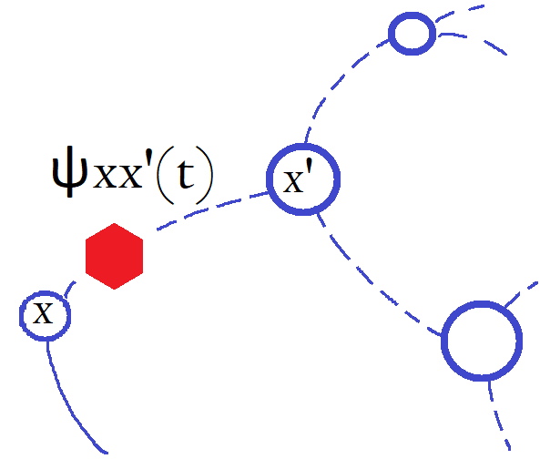
Figure 1: Illustration of the HCTRW model. A random walk jumps from site $x$ to $x^{\prime}$ during time, which is a random variable drawn from the probability density $\psi_{xx^{\prime}}(t)$.

II.2 Derivation of continuous limits for HCTRW dynamics

There are different ways to derive continuous limits from a random walk microscopic dynamics Landman1977 ; Klafter1980 ; Sokolov2007 . First we start with the heuristic derivation of the generalized master equation (GME). GME is the integro-differential equation that describes the evolution of a system in time Sokolov2011 , which is often used for derivation of Fokker-Planck diffusion equations. The generalized master equation is based on two balance conditions: (i) the local balance between the gain and loss fluxes at each site; (ii) the balance of transitions between any two sites, representing a particle conservation during jumps, e.g. the continuity property. These two conditions guarantee the probability conservation. We denote the probability to find a particle at time $t$ at site $\bar{x}$ and initially located at site $x_{0}$ by $P_{x_{0}\bar{x}}(t)$. Using the former condition (i) we represent the balance equation for the HCTRW as the standard balance equation between loss and gain fluxes $j^{\pm}_{\bar{x}}(t)$ in a site $\bar{x}$:

$$\frac{dP_{x_{0}\bar{x}}(t)}{dt}=j^{+}_{\bar{x}}(t)-j^{-}_{\bar{x}}(t).$$ (1)

The probability of a particle leaving $\bar{x}$ between $t$ and $t+dt$ is $j^{-}_{\bar{x}}(t)dt$. There are two possible scenarious: a particle leaving site $\bar{x}$ between $t$ and $t+dt$ either stays at site $\bar{x}$ from $t=0$ and in this case $\bar{x}=x_{0}$, or a particle arrives to site $\bar{x}$ at the later time $t^{\prime}$ such that $0<t^{\prime}<t$ for a discrete case. Therefore the loss flux is expressed as

$$j^{-}_{\bar{x}}(t)=\sum_{x^{\prime}}Q_{\bar{x}x^{\prime}}\psi_{\bar{x}x^{\prime}}(t)P_{x_{0}\bar{x}}(0)+$$ (2)

$$\int_{0}^{t}\sum_{x^{\prime}}Q_{\bar{x}x^{\prime}}\psi_{\bar{x}x^{\prime}}(t-t^{\prime})j^{+}_{\bar{x}}(t^{\prime})dt^{\prime},$$

where $P_{x_{0}\bar{x}}(0)$ is the initial probability distribution. In both sums we consider nodes $x^{\prime}$ adjacent to node $\bar{x}$, since the contribution to the total flux from each node $x^{\prime}$ is given by the term $Q_{\bar{x}x^{\prime}}\psi_{xx^{\prime}}(t-t^{\prime})j^{+}_{\bar{x}}(t^{\prime})$. For convenience we put $\mathcal{Q}_{\bar{x}}(t)=\sum_{x^{\prime}}Q_{\bar{x}x^{\prime}}\psi_{\bar{x}x^{\prime}}(t)$. Then the expression for the loss flux becomes:

$$j^{-}_{\bar{x}}(t)=\mathcal{Q}_{\bar{x}}(t)P_{x_{0}\bar{x}}(0)+\int_{0}^{t}\mathcal{Q}_{\bar{x}}(t-t^{\prime})j^{+}_{\bar{x}}(t^{\prime})dt^{\prime}.$$ (3)

Then the expression for the flux in Laplace domain is:

$$\tilde{j}^{-}_{\bar{x}}(s)=\tilde{\mathcal{Q}}_{\bar{x}}(s){P}_{x_{0}\bar{x}}(0)+$$ (4)

$$\tilde{\mathcal{Q}}_{\bar{x}}(s)(s\tilde{P}_{x_{0}\bar{x}}(s)-{P}_{x_{0}\bar{x}}(0)+\tilde{j}^{-}_{\bar{x}}(s)).$$

From here on the tilde denotes Laplace-transform of the corresponding function. The expression for $\tilde{j}^{-}_{\bar{x}}(s)$ allows us to express $j^{-}_{\bar{x}}(t)$ through ${P}_{x_{0}\bar{x}}(t)$ and $\mathcal{Q}_{\bar{x}}(t)$ in Laplace domain:

$$\tilde{j}^{-}_{\bar{x}}(s)=s\frac{\tilde{\mathcal{Q}}_{\bar{x}}(s)}{1-\tilde{\mathcal{Q}}_{\bar{x}}(s)}\tilde{P}_{x_{0}\bar{x}}(s)\equiv\tilde{\Phi}_{\bar{x}}(s)\tilde{P}_{x_{0}\bar{x}}(s),$$ (5)

where the memory kernel $\tilde{\Phi}_{\bar{x}}(s)$ is expressed through $\tilde{\mathcal{Q}}_{\bar{x}}(s)$, which intrinsically depends on travel time distributions $\psi_{\bar{x}x^{\prime}}(t)$ between ${\bar{x}}$ and neighboring sites $x^{\prime}$. The loss flux also intrinsically depends on a local structure of a network and temporal heterogeneities defined by the generalized transition matrix $Q(t)$ GrebTupikina . For convenience we introduce function $M_{x}(t)$, which in Laplace domain gives:

$$\tilde{M}_{\bar{x}}(s)=\frac{\tilde{\mathcal{Q}}_{\bar{x}}(s)}{1-\tilde{\mathcal{Q}}_{\bar{x}}(s)},$$ (6)

which we are using furthermore to dissect various generalized master equations.

The condition (ii) on the probability conservation of fluxes between sites can be written in the form, where the gain flux received at ${\bar{x}}$ consists from the loss fluxes from adjacent sites weighted by the transition probabilities:

$$j^{+}_{\bar{x}}(t)=\sum_{x^{\prime}}Q_{{\bar{x}}x^{\prime}}j^{-}_{x^{\prime}}(t).$$ (7)

Writing Eq. (7) in Laplace domain together with Eq. (1) gives us the final expression for GME in Laplace domain

$$s\tilde{P}_{x_{0}\bar{x}}(s)-P_{x_{0}\bar{x}}(0)=$$ (8)

$$\sum_{x^{\prime}}Q_{\bar{x}x^{\prime}}\Big{(}s\tilde{M}_{x^{\prime}}(s)\tilde{P}_{x_{0}x^{\prime}}(s)\Big{)}-s\tilde{M}_{\bar{x}}(s)\tilde{P}_{x_{0}\bar{x}}(s).$$

While in the real time domain we can write:

$$\dot{P}_{x_{0}\bar{x}}(t)=\sum_{x^{\prime}}Q_{\bar{x}x^{\prime}}\Big{(}\frac{d}{dt}\int_{0}^{t}M_{x^{\prime}}(t-t^{\prime})P_{x_{0}x^{\prime}}(t^{\prime})dt^{\prime}\Big{)}-$$ (9)

$$\frac{d}{dt}\int_{0}^{t}M_{\bar{x}}(t-t^{\prime})P_{x_{0}\bar{x}}(t^{\prime})dt^{\prime}.$$

For simplicity, we first consider GME for the HCTRW on a regular graph and put $Q_{\bar{x}x^{\prime}}=1/2$, if other value is not stated explicitly. For any $k$-regular graph with fixed degree $k$ for each node we set $Q_{\bar{x}x^{\prime}}=\frac{1}{k}$. Then from Eq. (II.2) we get the GME in a simpler form

$$\dot{P}_{x_{0}\bar{x}}(t)=\frac{d}{dt}\int_{0}^{t}\big{(}\frac{1}{2}\sum_{x^{\prime}=\bar{x}\pm 1}M_{x^{\prime}}(t-t^{\prime})P_{x_{0}x^{\prime}}(t^{\prime})-$$ (10)

$$-M_{\bar{x}}(t-t^{\prime})P_{x_{0}\bar{x}}(t^{\prime})\big{)}dt^{\prime}.$$

Further, in Section III we derive the continuous limits for various setups (or interpretations) of the HCTRW model.

III Interpretations of HCTRW

Here we introduce various setups (or interpretations) of the HCTRW model, depending on the definition of the travel time distributions $\psi_{\bar{x}x^{\prime}}(t)$, Fig. 1. We consider two phases of a jump of the HCTRW model: (1) when a random walk decides where to go with the fixed transition probability; (2) when a random walk decides how long does it take. All in all, we distinguish three different HCTRW model interpretations:
$\bullet$ The first (I) continuous HCTRW interpretation a random walk stays in node $\bar{x}$ during the travel time, which in this case is denoted as $\psi_{\bar{x}}(t)$, and then instantaneously jumps to $x^{\prime}$.
$\bullet$ The second (II) continuous HCTRW interpretation: a random walk arrives to a node $\bar{x}$ and stays on an edge between $\bar{x}$ and $x^{\prime}$ during time drawn from the probability density function $\psi_{\bar{x}x^{\prime}}(t)$.
$\bullet$ The third (III) continuous HCTRW interpretation: a random walk arrives to $x^{\prime}$ from $\bar{x}$ and waits at $x^{\prime}$ during time driven with the probability density function, in this case denoted as $\psi_{x^{\prime}}(t)$.

The interpretations defined above also correspond to different cases of, so-called, up- and down-times of links activations of stochastic temporal networks Petit2019 . Here we attempt to rigorously define the continuous limits of the HCTRW model and the term ”interpretation” (or ”continuous interpretation”) should be understood as a microscopic level of interpretation. The Langevin equation can be used to describe the separate characteristics of a physical system, necessary for homogeneous and heterogeneous systems. We note that in the context of the Langevin equation the term ”interpretation” was used in order to describe the inverse procedure to the aggregation Sokolov2010 .

III.1 First HCTRW interpretation

We start with the first HCTRW interpretation on one dimensional lattice, when the travel time distribution depends only on one node $\bar{x}$ (from where the HCTRW comes from) and not on $x^{\prime}$: $\psi_{\bar{x}x^{\prime}}(t)=\psi_{\bar{x}}(t)$. Then Eq. (6) becomes

$$\tilde{M}_{\bar{x}}(s)=\frac{\mathcal{Q}_{\bar{x}}(s)}{1-\mathcal{Q}_{\bar{x}}(s)}=\frac{\tilde{\psi}_{\bar{x}}(s)\sum_{x^{\prime}}Q_{\bar{x}x^{\prime}}}{1-\tilde{\psi}_{\bar{x}}(s)\sum_{x^{\prime}}Q_{\bar{x}x^{\prime}}}=\frac{\tilde{\psi}_{\bar{x}}(s)}{1-\tilde{\psi}_{\bar{x}}(s)}.$$

For the first HCTRW interpretation we consider various cases of dependence of $\psi_{\bar{x}}(t)$ and $\bar{x}$: (o) $\psi_{\bar{x}}(t)=\psi(t)$ for all nodes $\bar{x}$; (i) all travel time distributions are exponential with parameter depending on the node $\bar{x}$; (ii) all travel time distributions have finite moments; (iii) at least one moment of travel time distribution is infinite.

(o) The simplest case is when all travel time distributions are the same $\psi(t)$ for all nodes $\bar{x}$. Then Eq. (II.2) is transformed to the form:

$$\dot{P}_{x_{0}\bar{x}}(t)=\frac{d}{dt}\int_{0}^{t}\big{(}\frac{a^{2}}{2}\frac{M(t-t^{\prime})P_{x_{0}\bar{x}+1}(t^{\prime})}{a^{2}}-$$ (11)

$$\frac{-2M(t-t^{\prime})P_{x_{0}\bar{x}}(t^{\prime})+M(t-t^{\prime})P_{x_{0}\bar{x}-1}(t^{\prime})dt^{\prime}}{a^{2}}\big{)}$$ (12)

and then to the form of differential equation

$$\frac{d}{dt}P_{x_{0}x}(t)=\frac{a^{2}}{2}\frac{d^{2}}{dx^{2}}\frac{d}{dt}\int_{0}^{t}M(t-t^{\prime})P_{x_{0}x}(t^{\prime})dt^{\prime},$$ (13)

where $a$ denotes a distance between two neighboring sites of one dimensional lattice.

(i) The case when all travel times are exponential with parameter $\tau_{\bar{x}}$ $\tilde{\psi}_{\bar{x}}(s)=1/(1+s\tau_{\bar{x}})$ gives us then

$$\tilde{M}_{\bar{x}}(s)=\frac{1}{s\tau_{\bar{x}}}.$$ (14)

Assuming continuous dependence of $\tau_{\bar{x}}$ parameter from $\bar{x}$ and putting $D(\bar{x})=\frac{a^{2}}{2\tau_{\bar{x}}}$, Eq. (II.2) can be transformed to a continuous form of a diffusion equation in the Ito form, which coincides with the results obtained in Barkai ; Landman1977

$$\frac{d}{dt}P_{x_{0}x}(t)=\frac{d^{2}}{dx^{2}}D(x)P_{x_{0}x}(t),$$ (15)

where $D(x)=\lim_{\bar{x}\rightarrow x}\frac{a^{2}}{2\tau_{\bar{x}}}$. We note that this configuration mimics the kinetics of the trap model with exponential waiting times Sokolov2010 . The first interpretation is closely related to continuous limits for Markov jump processes Stroock .

(ii) In the case when all mean travel times are finite but not necessarily exponential, one can write the second order expansion valid for small $s$: $\tilde{\psi}_{\bar{x}}(s)=1-s\langle\tau_{\bar{x}}\rangle-s^{2}/2\langle\tau_{\bar{x}}\rangle^{2}+o(s^{2})$. Then the function $\tilde{M}_{\bar{x}}(s)$ is simply

$$\tilde{M}_{\bar{x}}(s)\propto\frac{1-s\langle\tau_{\bar{x}}\rangle-s^{2}/2\langle\tau_{\bar{x}}\rangle^{2}}{s\langle\tau_{\bar{x}}\rangle+s^{2}/2\langle\tau_{\bar{x}}\rangle^{2}},$$ (16)

which gives the correction in the real time domain $-\frac{1}{\langle\tau_{\bar{x}}\rangle}+e^{-t/\langle\tau_{\bar{x}}\rangle}+\delta(t)$, and differs from the terms in Eq. (14). Then from Eq. (II.2) we get:

$$s\tilde{P}_{x_{0}\bar{x}}(s)-P_{x_{0}\bar{x}}(0)=$$ (17)

$$\sum_{x^{\prime}}Q_{\bar{x}x^{\prime}}\Big{(}s\tilde{M}_{x^{\prime}}(s)\tilde{P}_{x_{0}x^{\prime}}(s)\Big{)}-s\tilde{M}_{\bar{x}}(s)\tilde{P}_{x_{0}\bar{x}}(s).$$

We can transform this to the form of differential equation with the integro-differential operators

$$\frac{d}{dt}P_{x_{0}x}(t)=\frac{a^{2}}{2}\frac{d^{2}}{dx^{2}}\frac{d}{dt}\int_{0}^{t}M_{x}(t-t^{\prime})P_{x_{0}x}(t^{\prime})dt^{\prime}.$$ (18)

The main difference between differential equations (13) and (18) is that in case (o) when $\psi_{\hat{x}}(t)=\psi(t)$ the function $M_{x}(t)$ is site-independent. Eq. (18) has more general form than the diffusion equation for homogeneous CTRW Barkai .

(iii) The last case is when at least one mean travel time is infinite. First we put all travel time distributions to be power laws with exponents coordinate-dependent $\alpha(x)$: $\psi_{\bar{x}}(t)=t^{-1-\alpha(\bar{x})}$, we get

$$M_{\bar{x}}(t)\propto\frac{1}{\langle\tau_{\bar{x}}\rangle}t^{-1+\alpha(x)}-\delta(t).$$ (19)

Then the diffusion equation has the integro-differential operators with parameter $\alpha$:

$$\frac{dP_{x}(t)}{dt}=\frac{d^{2}}{dx^{2}}(D(x)\textfrak{D}_{t}^{1-\alpha(x)}P_{x}(t))$$

where $\textfrak{D}^{1-\alpha(x)}_{t}$ is the generalization of the Riemann-Liouville derivative of order $1-\alpha(x)$:

$$\textfrak{D}^{1-\alpha(x)}_{t}(P_{x_{0}x}(t))=\frac{1}{\Gamma(1-\alpha(x))}\frac{d}{dt}\int_{0}^{t}\frac{P_{x_{0}x}(t^{\prime})dt^{\prime}}{(t-t^{\prime})^{\alpha(x)}}.$$ (20)

When all $\tilde{\psi}_{\bar{x}}(s)$ exhibit power law behaviour with the same scaling exponent $\alpha$: $\tilde{\psi}_{\bar{x}}(s)=1-s^{\alpha}\langle\tau_{\bar{x}}\rangle^{\alpha}+o(s^{\alpha})$, the function $\tilde{M}_{\bar{x}}(s)$ is:

$$\tilde{M}_{\bar{x}}(s)\propto\frac{1-s^{\alpha}\langle\tau^{\alpha}_{\bar{x}}\rangle}{s^{\alpha}\langle\tau_{\bar{x}}\rangle^{\alpha}},$$ (21)

which gives the differential form of the equation as in Chechkin2006 .

We consider the specific example of the equation with exponential travel times $\tilde{\psi}_{x}(s)=1/(1+s\tau(x))$ and temporal heterogeneities introduced $\tau(x)=\sin(x)$, as it was considered for the interval in GrebTupikina . Then Eq. (15) takes a form

$$\frac{d}{dt}P_{x_{0}x}(t)=\frac{d^{2}}{dx^{2}}\big{(}\frac{a^{2}}{2\sin(x)}P_{x_{0}x}(t)\big{)}$$ (22)

with the space-dependent diffusion coefficient.

III.2 Second HCTRW interpretation

In the second and third HCTRW interpretations the waiting time distribution $\tilde{\psi}_{\bar{x}}(s)$ depends on neighboring nodes of $\bar{x}$, while in the first interpretation $\tilde{\psi}_{\bar{x}}(s)$ depends on $\bar{x}$ only, section III.1. For the second and third interpretations the general form of GME Eq. (II.2) can be simplified:

$$s\tilde{P}_{x_{0}\bar{x}}(s)-P_{x_{0}\bar{x}}(0)=$$ (23)

$$s(\tilde{M}_{\bar{x}+1}(s)\tilde{P}_{x_{0}\bar{x}+1}(s)-\tilde{M}_{\bar{x}}(s)\tilde{P}_{x_{0}\bar{x}}(s))+$$

$$s(\tilde{M}_{\bar{x}-1}(s)\tilde{P}_{x_{0}\bar{x}}(s)-\tilde{M}_{\bar{x}}(s)\tilde{P}_{x_{0}\bar{x}}(s)).$$

Then after simplifying the right-hand side of the equation and taking the limit we come to the expression:

$$\lim_{a\rightarrow 0}\big{(}\frac{(\tilde{M}_{\bar{x}+1}(s)-\tilde{M}_{\bar{x}}(s))\tilde{P}_{x_{0}\bar{x}+1}(s)}{a^{2}}$$ (24)

$$-\frac{(\tilde{M}_{\bar{x}}(s)-\tilde{M}_{\bar{x}-1}(s))\tilde{P}_{x_{0}\bar{x}-1}(s)}{a^{2}}\big{)}=$$

$$\lim_{a\rightarrow 0}\frac{\tilde{M}_{\bar{x}+1}(s)-\tilde{M}_{\bar{x}}(s)}{a}\lim_{a\rightarrow 0}\frac{\tilde{P}_{x_{0}\bar{x}+1}(s)-\tilde{P}_{x_{0}\bar{x}-1}(s)}{a}.$$

Assuming a slow change of $\tilde{M}_{\bar{x}}(s)$ from $\bar{x}$ we can put: $\tilde{M}_{\bar{x}+1}(s)-\tilde{M}_{\bar{x}}(s)\approx\tilde{M}_{\bar{x}}(s)-\tilde{M}_{\bar{x}-1}(s)$. Then the evolution equation is:

$$s\tilde{P}_{x_{0}{x}}(s)-P_{x_{0}{x}}(0)=$$ (25)

$$a^{2}s\tilde{M}_{x}(s)\frac{d^{2}P_{x_{0}x}(s)}{dx^{2}}+a^{2}s\Big{(}\frac{d\tilde{M}_{x}(s)}{dx}\Big{)}\Big{(}\frac{dP_{x_{0}x}(s)}{dx}\Big{)}.$$

Then the right-hand side can be further transformed to

$$s\tilde{P}_{x_{0}{x}}(s)-P_{x_{0}{x}}(0)=\frac{d}{dx}\tilde{M}_{x}(s)\frac{d}{dx}\tilde{P}_{x_{0}x}(s).$$ (26)

Note that Eq. (26) differs from Eq. (15), obtained using general assumptions about $M_{\bar{x}}(t)$ properties and allowing a waiting time distribution to depend on $\bar{x},x^{\prime}$ nodes.

III.2.1 Second continuous HCTRW interpretation in one dimension

Here we consider the second continuous HCTRW interpretation for one-dimensional case. In this case a random walk spends in each site $\bar{x}$ time driven from the distribution $\psi_{\bar{x}x^{\prime}}(t)$, which depends on both $\bar{x},x^{\prime}$, hence in this case we can not use the assumption of locality as in the first interpretation. When a travel time distribution can be represented in a form of linear combination of functions $\psi_{\bar{x}x^{\prime}}(t)=\gamma_{1}\psi_{\bar{x}}(t)+\gamma_{2}\psi_{x^{\prime}}(t)$ for some parameter $\gamma$, this case can be analyzed using the first and third interpretations. For the symmetric case with equal $Q_{\bar{x}x^{\prime}}$ for all $x^{\prime}$ and fixed $\bar{x}$ we simply can write

$$\tilde{M}_{\bar{x}}(s)=\frac{\sum_{{x}^{\prime}=\bar{x}\pm 1}\tilde{\psi}_{\bar{x}x^{\prime}}(s)}{2-\sum_{{x}^{\prime}\bar{x}\pm 1}\tilde{\psi}_{\bar{x}x^{\prime}}(s)}.$$ (27)

Further we use the assumption of smoothness of $M_{\bar{x}}(t)$. We refer to calculations for the third interpretation in Subsection III.3 and define new functions $M^{\bar{x}+1}_{\bar{x}}(t)$, $M_{\bar{x}}(t)$. Coming to the continuous limit in Laplace domain

$$s\tilde{P}_{x_{0}x}(s)-{P}_{x_{0}x}(0)=\frac{d}{dx}sM_{x}(s)\frac{d}{dx}\tilde{P}_{x_{0}x}(s),$$ (28)

the right-hand side of which gives $D(x)\tilde{P}^{\prime\prime}_{x_{0}x}(s)+D^{\prime}(x)\tilde{P}^{\prime}_{x_{0}x}(s)$. Comparing Eq. 26 with Eq. (28) we deduce some specific properties of the second interpretation. Now as in the first interpretation we will consider several different cases for the travel time types.

(o) We start with the case when all mean travel times of $\tilde{\psi}_{\bar{x}x^{\prime}}(t)$ are finite $\langle\tau_{\bar{x}x^{\prime}}\rangle$: $\tilde{\psi}_{\bar{x}x^{\prime}}(s)=1-s\langle\tau_{\bar{x}x^{\prime}}\rangle+\frac{s^{2}}{2}\langle\tau_{\bar{x}x^{\prime}}\rangle^{2}+o(s^{2})$ for small $s$. When taking into account only first order terms we get:

$$M_{\bar{x}}(s)=\frac{1-s\hat{\tau}_{\bar{x}}}{s\hat{\tau}_{\bar{x}}},$$ (29)

where we call $\hat{\tau}_{\bar{x}}=(\langle\tau_{\bar{x}\bar{x}+1}\rangle+\langle\tau_{\bar{x}\bar{x}-1}\rangle)/2$. In this case then we get $M_{\bar{x}}(t)\approx 1/\hat{\tau}_{\bar{x}}-A(\hat{\tau}_{\bar{x}})\delta(t)$, where coefficient $A(\hat{\tau}_{\bar{x}})$ is set by higher order terms. Since $\hat{\tau}_{\bar{x}}$ depends on the neighbouring sites, we can use the assumption of slowly changing $M_{\bar{x}}(s)$ from $\bar{x}$. Therefore substituting these functions to Eq. (II.2) and using Taylor series we come to the continuous limit:

$$s\tilde{P}_{x_{0}\bar{x}}(s)-P_{x_{0}\bar{x}}(0)=$$ (30)

$$\sum_{x^{\prime}=\bar{x}\pm 1}\frac{1}{2}\Big{(}\frac{1-s\hat{\tau}_{x^{\prime}}}{\hat{\tau}_{x^{\prime}}}\tilde{P}_{x_{0}x^{\prime}}(s)\Big{)}-\frac{1-s\hat{\tau}_{\bar{x}}}{\hat{\tau}_{\bar{x}}}\tilde{P}_{x_{0}\bar{x}}(s).$$

This is the ”stepping stone” of the derivation for the second continuous HCTRW interpretation. We compare the diffusion coefficient from Eq. III.2.1 with the first interpretation, Eq. (14) with $D(\bar{x})=\frac{a^{2}}{2{\tau}_{\bar{x}}}$.

III.2.2 Second interpretation with exponential travel time distributions

Here we consider particular case of the second interpretation with the exponential travel time distribution. Similar case was considered in Bouchard , where transition rates $Q_{\bar{x}\bar{x}+1}$ have two parameters $D_{\bar{x}\bar{x}+1}$ and $F_{\bar{x}\bar{x}+1}$ We note that here we consider ME and calculations for GME will be done further. When the rate parameters depend on the starting and end points, then:

$$Q_{\bar{x}\bar{x}+1}=\frac{D_{\bar{x}\bar{x}+1}}{a^{2}}\exp(-\frac{aF_{\bar{x}\bar{x}+1}}{2\gamma D_{\bar{x}\bar{x}+1}}),$$ (31)

where $F_{\bar{x}\bar{x}+1}$ is microscopic parameter, related to the interaction with the medium, $a$ is the parameter of the lattice. Using the expansion in powers of $a$ we get:

$$\frac{d}{dt}P_{x_{0}\bar{x}+1}\approx$$ (32)

$$\frac{1}{a}\big{(}D_{\bar{x}\bar{x}+1}\frac{P_{x_{0}\bar{x}+1}-P_{x_{0}\bar{x}}}{a}-D_{\bar{x}-1\bar{x}}\frac{P_{x_{0}\bar{x}}-P_{x_{0}\bar{x}-1}}{a}\big{)}$$

$$+\frac{1}{a}\big{(}\frac{F_{\bar{x}-1\bar{x}}}{\gamma}\frac{P_{x_{0}\bar{x}+1}-P_{x_{0}\bar{x}}}{2}-\frac{F_{\bar{x}\bar{x}+1}}{\gamma}\frac{P_{x_{0}\bar{x}}-P_{x_{0}\bar{x}-1}}{2}\big{)}$$

$$+\frac{1}{8}\big{(}\frac{F^{2}_{\bar{x}\bar{x}+1}}{\gamma^{2}D_{\bar{x}\bar{x}+1}}(P_{x_{0}\bar{x}+1}-P_{x_{0}\bar{x}})$$

$$-\frac{F^{2}_{\bar{x}-1\bar{x}}}{\gamma^{2}D_{\bar{x}\bar{x}-1}}(P_{x_{0}\bar{x}}-P_{x_{0}\bar{x}-1})\big{)}$$

Then in the limit we get Fokker-Planck in the form

$$\frac{d}{dt}P_{x_{0}x}(t)=\frac{d}{dx}(-\frac{F(x)}{\gamma}P+D(x)\frac{d}{dx}P),$$ (33)

where we $D(x)=\lim_{\bar{x}\rightarrow x}\frac{a^{2}}{\tau_{\bar{x}+1}+\tau_{\bar{x}-1}}$.

In the case when the rate microscopic parameter $D$ depends only on one of the microscopic evaluation points, as in the asymmetric case Bouchard , e.g.:

$$Q_{\bar{x}\bar{x}+1}=\frac{D_{\bar{x}+1}}{a^{2}}\exp(-\frac{aF_{\bar{x}\bar{x}+1}}{2\gamma D_{\bar{x}+1}}),$$ (34)

$$Q_{\bar{x}+1\bar{x}}=\frac{D_{\bar{x}}}{a^{2}}\exp(-\frac{aF_{\bar{x}\bar{x}+1}}{2\gamma D_{\bar{x}}}).$$ (35)

From this we get

$$\frac{d}{dt}P_{x_{0}\bar{x}+1}\approx\frac{1}{a}\big{(}D_{\bar{x}+1}\frac{P_{x_{0}\bar{x}+1}-P_{x_{0}\bar{x}}}{a}-D_{\bar{x}}\frac{P_{x_{0}\bar{x}}-P_{x_{0}\bar{x}-1}}{a}\big{)}+$$ (36)

$$+\frac{1}{a}\big{(}\frac{F_{\bar{x}-1\bar{x}}}{\gamma}\frac{P_{x_{0}\bar{x}+1}-P_{x_{0}\bar{x}}}{2}-\frac{F_{\bar{x}\bar{x}+1}}{\gamma}\frac{P_{x_{0}\bar{x}}-P_{x_{0}\bar{x}-1}}{2}\big{)}+$$

$$+\frac{1}{8}\big{(}\frac{F^{2}_{\bar{x}\bar{x}+1}}{\gamma^{2}D_{\bar{x}+1}}(P_{x_{0}\bar{x}+1}-P_{x_{0}\bar{x}})-\frac{F^{2}_{\bar{x}-1\bar{x}}}{\gamma^{2}D_{\bar{x}}}(P_{x_{0}\bar{x}}-P_{x_{0}\bar{x}-1})\big{)}.$$

Then the corresponding Fokker-Planck should give the form

$$\frac{d}{dt}P(x,t)=\frac{d}{dx}(-\frac{F(x)}{\gamma}P(x,t)+\frac{d}{dx}D(x)P(x,t)),$$ (37)

which hence corresponds to another diffusion convention, the Stratonovich form for diffusion, related to kinetic interpretation, as noted in Sokolov2010 . Moreover, for different discrete models, the diffusion term can be written in the form:

$$\frac{d}{dx}(D(x)^{\alpha}\frac{d}{dx}D(x)^{1-\alpha}P),$$ (38)

where parameter $\alpha\in[0,1].$

III.3 Third HCTRW interpretation

Finally, we consider the third continuous interpretation of HCTRW, when each travel time distribution $\psi_{\bar{x}x^{\prime}}(t)$ depends only on the end point $x^{\prime}$, where the random walk jumps. For convenience, we first consider one-dimensional case and put the transition matrix $Q_{\bar{x}x^{\prime}}=1/2$. Then the expression for the function $M_{\bar{x}}(s)$ is expressed explicitly as the function of the neighboring sites of $\bar{x}$, using the derivations from Subsection II:

$$M_{\bar{x}}(s)=\frac{\sum_{x^{\prime}=\bar{x}\pm 1}\tilde{\psi}_{x^{\prime}}(s)}{2-\sum_{x^{\prime}=\bar{x}\pm 1}\tilde{\psi}_{x^{\prime}}(s)}.$$ (39)

When all travel time distributions are exponentials, we get:

$$M_{\bar{x}}(s)=\frac{s(\tau_{\bar{x}+1}+\tau_{\bar{x}-1})+2}{s(\tau_{\bar{x}+1}+\tau_{\bar{x}-1})+2s^{2}\tau_{\bar{x}+1}\tau_{\bar{x}-1}},$$ (40)

where kernel $M_{\bar{x}}(s)$ depends on local properties of neighboring nodes of $\bar{x}$. Inserting the Taylor series expansion for Eq. (40) we regroup components to see the difference with Eq. (14)

$$M_{\bar{x}}(s)=\frac{1}{s\tau_{\bar{x}}}(1+s\delta\phi_{\bar{x}})(1-s\delta\phi_{\bar{x}})(1-\frac{a^{2}\phi^{\prime\prime}}{2\phi_{\bar{x}}}),$$ (41)

where we denoted $\tau_{x}=\delta\phi_{x}$ so that later we can use the standard notations $D=\frac{a^{2}}{2\delta}$. Directly from Eq. (40) we get

$$M_{\bar{x}}(t)=\frac{2}{\tau_{\bar{x}+1}+\tau_{\bar{x}-1}}+$$ (42)

$$e^{-t\frac{\tau_{\bar{x}+1}+\tau_{\bar{x}-1}}{\tau_{\bar{x}+1}\tau_{\bar{x}-1}}}\frac{\tau_{\bar{x}+1}-\tau_{\bar{x}-1}}{2\tau_{\bar{x}+1}\tau_{\bar{x}-1}(\tau_{\bar{x}+1}+\tau_{\bar{x}-1})},$$

where in the limit the second term on the right hand side vanishes to zero. The expansion of $\tau_{x}$ gives us: $\tau_{\bar{x}+1}\approx\tau_{\bar{x}}+a\tau^{\prime}_{\bar{x}}+a^{2}/2\tau^{\prime\prime}_{\bar{x}}$. Using the expression for the function $M_{x}(t)$ from Eq. (40) we get the equation with two convolutions in the real time domain:

$$\frac{dP_{x_{0}x}(t)}{dt}=M_{x}(t)P_{x_{0}x}^{\prime\prime}(t)+M_{x}^{\prime}(t)P_{x_{0}x}^{\prime}(t).$$ (43)

Note that for the first interpretation of continuous HCTRW the function $M_{x}=\lim_{\bar{x}\rightarrow x}\frac{a^{2}}{2\tau_{\bar{x}}}$ for the exponential travel time distributions, Eq. (15). We regroup components so that the final expression becomes:

$$\frac{dP_{x_{0}x}(t)}{dt}=\frac{dD(x)}{dx}\frac{dP_{x_{0}x}(t)}{dx},$$ (44)

where the right hand side transforms to $D(x)P_{x_{0}x}^{\prime\prime}(t)+D^{\prime}(x)P_{x_{0}x}^{\prime}(t)$. For the exponential travel times $D(x)=a^{2}/(2\tau(x))$. Or in Laplace domain:

$$s\tilde{P}_{x_{0}x}(s)-P_{x_{0}x}(0)=\frac{dD(x)}{dx}\frac{d\tilde{P}_{x_{0}x}(s)}{dx},$$ (45)

the right-hand side of which can be expressed as $D(x)\tilde{P}^{\prime\prime}_{x_{0}x}(s)+D^{\prime}(x)\tilde{P}^{\prime}_{x_{0}x}(s)$. Different way to calculate the continuous limits of GME is using the Taylor series of functions from Eq. (II.2):

$$\psi_{\bar{x}\pm 1}(t)=\psi_{\bar{x}}(t)\pm a\psi_{\bar{x}}(t)^{\prime}+a^{2}/2\psi_{\bar{x}}(t)^{\prime\prime},$$

where $a$ is a lattice parameter. Then

$$\tilde{P}_{x_{0}\bar{x}+1}(s)\approx\tilde{P}_{x_{0}\bar{x}}(s)+a\tilde{P}^{\prime}_{x_{0}\bar{x}}(s)+\frac{a^{2}}{2}\tilde{P}^{\prime\prime}_{x_{0}\bar{x}}(s),$$ (46)

where higher order terms can be neglected. Then we regroup components in Eq. (II.2) such that the first and second derivative in $x$ of $\tilde{P}_{x_{0}x}(s)$ from Eq. (46) are separated. We substitute Taylor expansion for functions in Eq. (II.2) to get for the one-dimensional symmetric case ($Q_{\bar{x}\pm 1}=1/2$):

$$s\tilde{P}_{x_{0}\bar{x}}(s)-\tilde{P}_{x_{0}\bar{x}}(0)=$$ (47)

$$\frac{1}{2}\sum_{x^{\prime}=\bar{x}\pm 1}\Big{(}sM_{x^{\prime}}(s)\tilde{P}_{x_{0}x^{\prime}}(s)\Big{)}-sM_{\bar{x}}(s)\tilde{P}_{x_{0}\bar{x}}(s).$$

The right-hand side after regrouping components gives

$$\frac{1}{2}\Big{(}sM_{\bar{x}+1}(s)(P_{x_{0}\bar{x}}(s)+aP_{x_{0}\bar{x}}^{\prime}(s)+a^{2}/2P_{x_{0}\bar{x}}^{\prime\prime}(s))+$$ (48)

$$sM_{\bar{x}-1}(s)(P_{x_{0}\bar{x}}(s)-aP_{x_{0}\bar{x}}^{\prime}(s)+a^{2}/2P_{x_{0}\bar{x}}^{\prime\prime}(s))\Big{)}-$$

$$-sM_{\bar{x}}(s)P_{x_{0}\bar{x}}(s)=$$

$$\frac{1}{2}\Big{(}sM_{\bar{x}+1}(s)(P_{x_{0}\bar{x}}(s)+aP_{x_{0}\bar{x}}^{\prime}(s)+a^{2}/2P_{x_{0}\bar{x}}^{\prime\prime}(s))-$$

$$-sM_{\bar{x}}(s)P_{x_{0}\bar{x}}(s))+$$

$$(sM_{\bar{x}-1}(s)(P_{x_{0}\bar{x}}(s)-aP_{x_{0}\bar{x}}^{\prime}(s)+$$

$$a^{2}/2P_{x_{0}\bar{x}}^{\prime\prime}(s))-sM_{\bar{x}}(s)P_{x_{0}\bar{x}}(s)\Big{)}.$$

Then we transform Eq. (III.3) by combining together the derivatives of the same order:

$$s\tilde{P}_{x_{0}\bar{x}}(s)-\tilde{P}_{x_{0}\bar{x}}(0)=$$ (49)

$$A_{\bar{x}}(s)P_{x_{0}\bar{x}(s)}+B_{\bar{x}}(s)P_{x_{0}\bar{x}}^{\prime}(s)+C_{\bar{x}}(s)P_{x_{0}\bar{x}}^{\prime\prime}(s),$$

where each coefficient is expressed as follows:

$$A_{\bar{x}}(s)=\frac{a^{2}s}{2}M_{\bar{x}}^{\prime\prime}(s),$$ (50)

$$B_{\bar{x}}(s)=a^{2}sM_{\bar{x}}^{\prime}(s),$$ (51)

$$C_{\bar{x}}(s)=\frac{a^{2}s}{2}(M_{\bar{x}}(s)+\frac{a^{2}}{2}M_{\bar{x}}^{\prime\prime}(s)),$$ (52)

where from the last equation for $C$ we eliminate later the component $\frac{a^{2}}{2}M_{\bar{x}}^{\prime\prime}(s)$.

We also note that the HCTRW with travel times $\psi_{\bar{x}x^{\prime}}(t)=\psi_{x^{\prime}}(t)$ can be considered as the limiting case of the second interpretation for $\alpha\rightarrow 0$ in $\psi_{\bar{x}x^{\prime}}(t)=\psi(\alpha\bar{x}+(1-\alpha)x^{\prime},t)$. Then by making travel times to be driven from exponential distributions, the HCTRW can be mapped to the so-called accordion model Sokolov2010 .

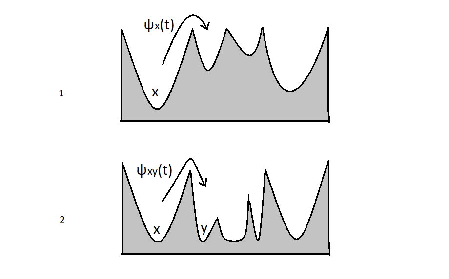
Figure 2: Illustration of connection between the HCTRW model an the trap model (1) or barrier model (2).

IV Discussions

In this paper we derived studied the continuous limits of heterogeneous continuous time random walk model (notation used in the text is HCTRW). We derived the generalized master equation for the HCTRW model and considered.

Previously, continuous limits of random walk models were considered for various models of stochastic processes. Dynamics of homogeneous CTRW model on a lattice and continuous limits for homogeneous CTRW on lattices were considered in Chechkin2006 . In Angstmann2015 the Generalized Master Equation (GME) for discrete time random walk was considered for various random walk models. In Lambiotte2011 the framework for continuous limits for CTRW model was developed. The diffusion coefficient, in general, depends on a combination of two kinetic parameters Sokolov2010 : mean free path and correlation time. Using parametrisation as in Sokolov2010 one can encode diffusion in inhomogeneous medium. Connection between the Langevin and Fokker-Planck equations, as well as the interpretations of Langevin equation, lead to various open questions, discussed in Pavliotis ; Kampen1981 ; Klafter1980 ; Sokolov2010 . As it was found in Serov , when diffusivity is not uniform, overdamped Langevin equation’s solution depends on the interpretation of stochastic term that appears in it.

In section III of our manuscript we considered the continuous HCTRW model starting with special cases of HCTRW in 1D. Calculations from Section II were made for the HCTRW without specification of underlying graph type. In particular, we studied the GME for HCTRW on tree graphs (the most straightforward generalisation of a linear graph), on lattice graphs. If a graph is a regular lattice with $\deg(i)=const$ $\forall i$, then Eq. (II.2) can be continuazed using methods described above. However for non-regular graphs this procedure should be done differently. Another question is setting HCTRW model on a particular type of graph with temporal structure $\tau(x)$ so that the continuous version would satisfy the diffusion equation

$$\frac{dP_{x_{0}x}(t)}{dt}=\frac{d}{dx}\mathcal{D}\frac{dP_{x_{0}x}(t)}{dt},$$ (53)

where $\mathcal{D}=diag(D_{1},...D_{N})$ is the diffusion tensor, corresponding to the isotropic inhomogeneous $N$-dimensional media with $D_{i}\neq D_{j},i\neq j$.

Moreover, in our manuscript we discuss the question about the relation between macroscopic view encoded in HCTRW interpretations and microscopic properties of the HCTRW model. First, we showed that the results for homogeneous cases of the HCTRW model, when all travel time distributions are the same, correspond well to the results from Chechkin2006 . Then in Section III we derived diffusion equations, which generalize some previous findings on continuous limits for homogeneous random walk models Barkai and heterogeneous random walk model GrebTupikina . Moreover, this allows us to study the influence of microscopic heterogeneity, encoded through travel time distributions, on the macroscopic level of diffusion. The GME for homogeneous and heterogeneous cases of HCTRW, derived in the manuscript, coincides well with the GME found in Kenkre1973 . In subsection III.3 we considered less general case, when travel time distributions depend only on one site $\psi_{\bar{x}x^{\prime}}=\psi_{x^{\prime}}$ and derived kernel functions for exponential travel time distributions. Comparing memory kernels of integro-differential operators allows us to compare diffusion equations. In particular, we propose HCTRW continuous limits conjecture about the relation between the HCTRW interpretations and various formalisms of diffusion equation. The HCTRW continuous limits conjecture can be formulated as follows: Ito formalism corresponds to the HCTRW model with travel time distributions $\psi_{\bar{x}x^{\prime}}$ depending only on nodes, where a random walk starts; Hänggi-Klimontovich - when $\psi_{\bar{x}x^{\prime}}$ is evaluated only in nodes $x^{\prime}$, where a random walk ends; Stratonovich - when $\psi_{\bar{x}x^{\prime}}$ is evaluated in both nodes, or in function from both nodes, e.g. $(\bar{x}+x^{\prime})/2$. New travel time distributions can be set, for instance, as $\psi_{\bar{x}x^{\prime}}(t)=\psi(\alpha x+(1-\alpha)x^{\prime},t)$. The first interpretation of HCTRW can be mapped to the CTRW model with $\psi_{\bar{x}}(t)$, where travel time distribution depends only on a starting point $\bar{x}$ and not on a node $x^{\prime}$.

IV.1 Langevin equation and SDE

Another important class of models for studying diffusion formalisms are so-called barrier and accordion models Sokolov2010 , where often you can use distribution of potential $U(x)$ and distribution of diffusion coefficients $D(x)$. When $U(x)$ has local minimums of the same height, we obtain a stationary distribution with a particle staying on the same height. Hence for barrier and accordion models we get completely different behaviour (Stratonovich or Hänggi), than for a trap model (Ito). Another important argument about continuous limits of the HCTRW model is that initially travel time distributions $\psi_{xx^{\prime}}(t)$ do not depend on a form of matrix entries $Q_{xx^{\prime}}$, although these entries can be independent, or be interrelated. Transition matrix entries $Q_{xx^{\prime}}$, in fact, can be related to the form of transition probability densities $\psi_{xx^{\prime}}(t)$. In Langevin equation

$$\dot{x}(t)=f(x)+g(x,t)l(t)$$ (54)

function $f(x)$ and $g(x)$ are two given functions, $l(t)$ is the rapid fluctuations. As it is pointed out in Kampen1981 the proper physical meaning should be given and we can distinguish the formalisms as follows. According to stochastic differential equation (SDE) above, each pulse in $l(t)$ leads to a jump in $x$. That has an effect that a value $x$ to be used in $g(x,t)$ is undetermined (and hence also a size of a jump). The general form of Fokker-Planck equation (FP) can be written as:

$$\frac{dP_{x_{0}x}(s)}{dt}=\frac{d}{dx}\big{[}-f(x)P_{x_{0}x}(s)+$$ (55)

$$\alpha(\frac{d}{dx}D(x))P_{x_{0}x}(s)+D\frac{dP_{x_{0}x}(s)}{dx}\big{]},$$

where different values of $\alpha$ correspond to: Hänggi formalism for $\alpha=0$, Stratonovich for $\alpha=1/2$, and Ito for $\alpha=1$. As it was stressed in Sokolov2010 , the fact that $\alpha$ mathematically defines the position of a sampling point within the integration interval, is quite secondary and has essentially to do not with (non)-anticipation but with spacial symmetries of transition rates. However for now the question stays, which formalism is more suitable for which random walk. In relation to this we briefly discuss below the role of symmetries and random walk transition rates. It is known that Ito integral is mathematically convenient to use Gardiner and that its martingale property allows to simplify derivation of Fokker-Planck equation from SDE. However physically this choice is not always motivated, since in the physical system a term $l(t)$ from Langevin equation may not necessarily be the white noise Volpe with finite correlation time.

IV.2 Discussions of the HCTRW interpretations

The first interpretation of the HCTRW model was discussed in detail in Section IV, therefore we start with the second interpretation. The second interpretation of the HCTRW model with the exponential travel times can be mapped to the barrier model Thiel2016 . Then the arguments from Sokolov2010 for the barrier model help us to show that the second continuous HCTRW interpretation corresponds to Stratonovich formalism. In the original barrier model Bouchard the transition rates depend on the barrier between nodes: $\omega_{0}q^{-\beta U_{B}(x_{i},x^{\prime})}$, where $U_{B}(x_{i},x^{\prime})$ is the barrier energy between nodes $x_{i}$ and $x^{\prime}$. If the nodes would be exchanged, no changes in the equilibrium distribution $p_{eq}$ would take place. This brings the argument that a barrier model urges for Hänggi-Klimontovich interpretation of the corresponding Langevin equation. The main difference between the barrier and the trap model, illustrated on Fig. 2, is that in the barrier model each node has zero potential. In Fig. 2 we illustrate the one dimensional barrier and trap models, which can be viewed as particular cases of HCTRW. The relation between the trap model Sokolov2010 and the HCTRW should be explored in more details elsewhere. Moreover, it can be used for investigation of correspondence between conventions.

V Conclusions

In this manuscript we presented the possible generalisation of the HCTRW model in continuous space and time. Moreover, we describe in details possible relations between continuous and discrete quantities of RW, such as waiting time (or travel time) distributions $\Psi_{\bar{x}}(t)$ GrebTupikina , and kernel functions $\sum_{x^{\prime}}Q_{\bar{x}x^{\prime}}\psi_{\bar{x}x^{\prime}}(t)=\mathcal{Q}_{\bar{x}}(t)$. This allows to open discussions on connections between discrete (in space) random walks with their continuous analogue of diffusion processes. General analysis of continuous limits of random walk models on graphs deepens connections between kinetic properties and intrinsic quantities of diffusion equations.

VI Outlook

As an outlook we plan to work on the derivation for a general case of second continuous HCTRW interpretation. In general, the HCTRW model and its continuous interpretations can be studied in various contexts, for instance on infinite graphs with locally finite properties: $\deg_{\bar{x}}<\infty$ $\forall\bar{x}$ of a graph. Another point to consider is the case of HCTRW with various waiting time distributions, such as Sibuya distribution Angstmann2015 , which could lead to interesting specific properties of diffusion equation. On another hand, following standard derivation of the Montroll-Weiss equation montroll1965 one can also study the non-markovian nature on the generalized master equation Hoffmann .

An interesting special case to consider is the HCTRW model, where $Q_{xx^{\prime}}$ transition matrix elements also depend on form of functional matrix entries $\psi_{xx^{\prime}}(t)$, as it was also considered in a different context in the work on barrier models. One of the possible applications of the continuous limits of HCTRW to real-world systems includes the models with permeable barriers and the model with the space-dependent diffusion coefficient Lanoissele . As for other possible applications the fractional equations for heterogeneous HCTRW can be also applied to the fractional diffusion of ion channel gating Goychuk2004 . Studying spectral properties of infinite graphs Mohar1989 , on which HCTRW takes place, is another way to study continuous version of HCTRW.

The relation between various formalisms of diffusion equation and continuous interpretations of HCTRW can be investigated further. In particular, Ito formalism in for the HCTRW - when $\psi_{\bar{x}x^{\prime}}$ depends only on $\bar{x}$; Hanggi-Klimontovich - when $\psi_{\bar{x}x^{\prime}}$ is evaluated only on $x^{\prime}$; Stratonovich - when $\psi_{\bar{x}x^{\prime}}$ is evaluated in between, i.e. in $(\bar{x}+x^{\prime})/2$. Other forms of travel time distribution can be set, for instance, as $\psi_{\bar{x}x^{\prime}}(t)=\psi(\alpha x+(1-\alpha)x^{\prime},t)$. The first interpretation of HCTRW can be mapped to the CTRW with $\psi_{\bar{x}}(t)$, where the travel time depends only on the starting point $\bar{x}$ and not on $x^{\prime}$. Note, that such mapping between HCTRW given by set of $\psi_{\bar{x}}(t)$ and $\psi_{\bar{x}x^{\prime}}(t)$ is not bijective. In order to come from the general setup of HCTRW to the first interpretation one can also put $\psi_{\bar{x}}(t)=n_{c}\sum_{x^{\prime}}\psi_{\bar{x}x^{\prime}}(t)$, where $n_{c}$ is the normalisation constant.

Acknowledgements: L.T. thanks Denis S. Grebenkov from Laboratoire de Physique de la Matière Condensée (UMR 7643), CNRS – Ecole Polytechnique, 91128 Palaiseau, France for inspiration and discussions of the main ideas of the manuscript. L.T. also acknowledges project http://inadilic.fr/ and the support under Grant No. ANR-13-JSV5-0006-01 of the French National Research Agency. L.T. thanks support of Centre of Research and Interdisciplinarity in France and personally A.Serov, C.Vestergaard, G. Volpe and Y. Lanoissele for relevant suggestions of citations.

References

- (1) E. Agliari, Phys. Rev. E, 77, 011128 (2008)
- (2) C.N. Angstmann, I.C. Donnelly, B.I. Henry, J.A. Nichols, Journal of Computational Physics, 293 C, 53-69 (2015)
- (3) V. Balakrishnan, M. Khantha, Pramana 21, 3, 111-122 (1983)
- (4) E. Barkai, Chem. Phys. 284, 13-27 (2008)
- (5) O. Benichou, D. S. Grebenkov, P. E. Levitz, C. Loverdo,and R. Voituriez, Journal of Statistical Physics 142, 657 (2011).
- (6) B. Berkowitz, H. Scher, and S. E. Silliman, Water Resour.Res 36, 149 (2000).
- (7) J.-P. Bouchaud, A. Georges, Physics Reports, 195, 4-5, 127-293 (1990).
- (8) A. Chechkin, R. Gorenflo, I.M.Sokolov, J.Phys.A. 38, L679–L684 (2005)
- (9) C. Chmelik, J. Kaerger, Microporous and Mesoporous Materials, 225, 128-132 (2016)
- (10) T. C. Choy, International Series of Monographs on Physics (Oxford University Press, New York, 1999)
- (11) J-C.Delvenne, R.Lambiotte, L.Rocha, Nature Communications 6:7366 (2015)
- (12) W. Feller, John Willey, Vol.1, 3 ed. (1970)
- (13) M. Filoche, S. Mayboroda, PNAS, 109, 37 (2012).
- (14) C. Gardiner, Springer Verlag, Springer Series in Synergetics (13) (2009)
- (15) I. Goychuk, P. Haenggi, Phys. Rev. E 70, 051915 (2004)
- (16) I. Goychuk, Phys. Rev. E 80, 046125 (2009)
- (17) C. Grabow, M. Timme, PRL (2012)
- (18) D. Grebenkov, Research summary for defending Habilitation for Research Supervision (HDR), (2009)
- (19) D. Grebenkov, L. Tupikina, Phys. Rev. E, 012148, 97 (2018)
- (20) D. Grebenkov, Jour. of Phys. A: Mathematical and Theoretical, 48, 013001, 1 (2015).
- (21) R. Hilfer, L. Anton, Phys. Rev. E (1995)
- (22) T. Hoffmann, M.A. Porter, R. Lambiotte, arxiv, 1306.0715 (2013)
- (23) T. Hoffmann, M.A. Porter, R. Lambiotte, Phys. Rev. E, 86, 046102 (2011)
- (24) B. Hughes, (Clarendon, Oxford, 1995)
- (25) F. Ianelli et al. Phys. Rev. E 95, 012313 (2017)
- (26) A. Julaiti, W. Bin, and Z. Zhang, J. Chem. Phys. 138, 204116 (2013)
- (27) N. Van Kampen, North.Holland Press (1981)
- (28) N. Van Kampen, J. Stat.Phys. 24. 1 (1981)
- (29) J. Kärger, Handbook of Zeolite Science and Technology 341 (2003).
- (30) V. Kenkre, E. Montroll, M. Schlesinger J. Stat.Phys 9:45 (1973)
- (31) J. Klafter, R. Silbey, Phys. Rev. L, 44 2 (1980).
- (32) J. Klafter, I. M. Sokolov, Oxford Uni.Press (2011).
- (33) D. Kondrashova et al., Nature 7:40207 (2017)
- (34) U. Landman, E. Montroll, J. Schlessinger, Proc. Nat. Acad. Sci. USA, 74(2):430-3. (1977)
- (35) Y.Lanoissele, D. Grebenkov J. Phys. A: Math. Theor. 51 145602 (2018)
- (36) J. Lin, Z. Zhang, PRE, 87, 062140 (2013)
- (37) J. Machta, Phys. Rev. B 24, 5260 (1981)
- (38) R. Metzler, J. Klafter, and I. M. Sokolov, Physical Review E 58, 1621 (1998).
- (39) P. V. Mieghem, Graph spectra, Cambridge University Press, (2011).
- (40) B. Mohar, Woess, Bull. London Math. Soc. 21 (1989)
- (41) E. Montroll and H. Scher, Journal of Statistical Physics 9, 101 (1973).
- (42) E. Montroll and G. Weiss, Journal of Mathematical Physics 6, 167 (1965).
- (43) S. De Nigris, T. Carletti, R. Lambiotte, Phys. Rev. E, 2017 - APS (2017)
- (44) J. Noh, H. Rieger, Phys. Rev. Lett. , 92, 118701 (2004)
- (45) S. Orzel, A. Weron Journal of Statistical Mechanics: Theory and Experiment (2011)
- (46) G. Pavliotis, Springer, Texts in Applied mathematics (2014)
- (47) N. Perra, B. Gonçalves, R. Pastor-Satorras, A. Vespignani, Scientific Reports, 2, 469 (2012)
- (48) J.Petit, R. Lambiotte, T. Carletti arxiv 1903.07453 (2019)
- (49) S. Redner, Cambridge Uni Press, vol. 70 (2002)
- (50) M. Sahimi, Phys.Rev.E, 85, 016316 (2012)
- (51) J. Saramaki and P. Holme, EPJ B 88 (2015)
- (52) H. Scher and M. Lax, Phys. Rev. B 7, 4491 (1973)
- (53) R. Schumer, A. Benson, and M. M. Meerschaert, Water Resour. Res., 39(10), 1296 (2003)
- (54) A S. Serov, F. Laurent, C. Floderer, K. Perronet, C. Favard, Delphine Muriaux, C. L. Vestergaard, J.B. Masson Scientific Reports, 10, 3783 (2020)
- (55) E.B. Postnikov, A. Chechkin, I.M. Sokolov, New J. Phys. 111573 (2018)
- (56) I. M. Sokolov, Chem.Phys. 375, 359-363 (2010)
- (57) I. Sokolov, J.Klafter, PRL, 97, 140602 (2006)
- (58) I. M. Sokolov, J. Klafter, Chaos, Fractals 81-86 (2007)
- (59) F. Spitzer, vol. 1, Springer, New York, Berlin, Heidelberg, (2001)
- (60) D. Stroock, Springer-Verlag, Berlin, Heidelberg (2005)
- (61) F. Thiel and I. M. Sokolov, Phys. Rev. E 95(2), 022108 (2016)
- (62) L. N. Trefethen and M. Embree, Princeton, NJ Princeton University Press (2005)
- (63) L. Tupikina, D. Grebenkov, arxiv, 1811.05913, Appl.Netw.Jour. (2019)
- (64) G. Volpe and J. Wehr, V. 79, 5 Reports on Progress in Physics (2016)