Weakly-correlated synapses promote dimension reduction in deep neural networks

Abstract

By controlling synaptic and neural correlations, deep learning has achieved empirical successes in improving classification performances. How synaptic correlations affect neural correlations to produce disentangled hidden representations remains elusive. Here we propose a simplified model of dimension reduction, taking into account pairwise correlations among synapses, to reveal the mechanism underlying how the synaptic correlations affect dimension reduction. Our theory determines the synaptic-correlation scaling form requiring only mathematical self-consistency, for both binary and continuous synapses. The theory also predicts that weakly-correlated synapses encourage dimension reduction compared to their orthogonal counterparts. In addition, these synapses slow down the decorrelation process along the network depth. These two computational roles are explained by the proposed mean-field equation. The theoretical predictions are in excellent agreement with numerical simulations, and the key features are also captured by a deep learning with Hebbian rules.

Introduction.— Neural correlation is a common characteristic in most neural computations [1], playing vital roles in stimulus coding [2, 3], information storage [4] and various cognition tasks that can be implemented by recurrent neural networks [5, 6]. Neural correlation was recently shown by a mean-field theory [7] to be able to manipulate the dimensionality of layered representations in deep computations, which was empirically revealed to be a fundamental process in deep artificial neural networks [8]. This theory demonstrates that a compact neural representation with weak neural correlations is an emergent behavior of layered neural networks whose synaptic weights are independently and identically distributed. However, in real cortical circuits, synaptic weights among neurons, even in the same layer, may not be ideally independent with each other [9, 10, 4, 11], perhaps mainly due to biological synaptic plasticity [4, 11]. On the other hand, a recent theoretical study of unsupervised feature learning predicts that weakly-correlated synapses promote unsupervised concept-formation by reducing the necessary sensory data samples [12, 13]. Therefore, in what exact way a weak correlation among synapses affects the emergent behavior of layered neural networks remains unknown.

In particular, suppression of unwanted variability in sensory inputs [14], compact representation of invariance (generalization to novel context) [15], and the feature selectivity (discrimination ability of neural representation) [16] may be closely related to an appropriate neural dimensionality, which keeps only relevant informative components spanning a robust neural subspace [6]. Therefore, clarifying how synaptic correlations affect neural correlations and further the neural process underlying the transformation of representation dimensionality becomes fundamentally important.

To reveal the mechanism underlying how the synaptic correlations affect compact neural representations, we consider deep neural networks that realize a layer-wise transformation of sensory inputs. All in-coming synapses to a hidden neuron form a receptive field (RF) of that hidden neuron. The correlation among synapses is modeled by the inter-RF correlation (Fig. 1). We do not need a prior knowledge about the synaptic correlation strength. In fact, our mean-field theory yields different scaling behaviors of synaptic correlation with respect to the number of neurons at each layer, for both binary and continuous synaptic weights. The scaling behaviors are exactly a requirement of mathematically well-defined dimensionality.

Compared to the previous work of orthogonal weights [7], our current model reveals richer ways of controlling dimensionality of neural representations, i.e., the dimensionality can be tuned layer by layer in both additive and multiplicative manners. Each manner can be analytically understood in the mean-field limit. The theory predicts that, according to the scaling, the weak correlation among inter-RF synapses is able to promote dimension reduction in deep neural networks. In addition, these synapses slow down the neural decorrelation process along the network hierarchy. Therefore, our theory provides deep insights towards understanding how synaptic correlations shape compact neural representations in deep neural networks.

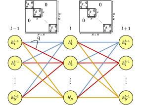
Figure 1: (Color online) Schematic illustration of a deep neural network with correlated synapses. The deep neural network carries out a layer-wise transformation of a sensory input. During the transformation, a cascade of internal representations ($\{\mathbf{h}^{l}\}$) are generated by the correlated synapses, with the covariance structure specified by the matrix above the layer. $g$ characterizes the variance of synaptic weights, while the diagonal block characterizes the inter-receptive-field correlation among corresponding synapses (different line colors), and $q$ specifies the synaptic correlation strength. We do not know a priori the exact scaling form of $q$, which is self-consistently determined by our theory.

Model.— A deep neural network is composed of multiple layers of non-linear transformation of sensory inputs (e.g., natural images). The depth of the network is defined as the number of hidden layers ($d$), and the width of each layer is defined by the number of neurons at that layer. For simplicity, we assume an equal width ($N$) in this study. To specify weights between $l-1$ and $l$-th layers, we define a weight matrix $\mathbf{w}^{l}$ whose $i$-th row corresponds to incoming connections to the neuron $i$ at the higher layer (so-called the receptive field of the neuron $i$). Firing biases of neurons at the $l$-th layer are denoted by $\mathbf{b}^{l}$. The input data are transformed through consecutive hidden representations denoted by $\mathbf{h}^{l}$ ($l=1,\cdots,d$), in which each entry $h_{i}^{l}$ defines a non-linear transformation of its pre-activation $z_{i}^{l}\equiv[\mathbf{w}^{l}\mathbf{h}^{l-1}]_{i}+b_{i}^{l}$, as $h_{i}^{l}=\phi(z_{i}^{l})$. Without loss of generality, we use the non-linear transfer function $\phi(x)=\tanh(x)$.

To take into account inter-RF correlations, we specify the covariance structure as $\overline{w_{ik}^{l}w_{jk}^{l}}=q$ for $i\neq j$, and $\overline{(w_{ik}^{l})^{2}}=g^{2}/N$ for continuous weights, while $\overline{(w_{ik}^{l})^{2}}=1$ for binary weights ($\pm 1$) (see Fig. 1). The weight has zero mean. The bias follows $\mathcal{N}(0,\sigma_{b})$. The orthogonal RF case was studied in a recent work [7] that demonstrates mechanisms of dimension reduction in deep neural networks of continuous weights. Here, we extend the analysis to the non-orthogonal case, and do not enforce any scaling constraint a priori to the correlation level $q$. The role of $q$ in dimension reduction is determined in a self-consistent way. Note that we do not assume any prescribed correlations of intra-RF weights for simplicity. In the current setting, the weight matrix $\mathbf{w}^{l}$ is more highly structured than in the orthogonal case, resembling qualitatively what occurs in a biological neural circuit [10, 11].

To define the computational task, we consider a random input ensemble from which each input sample is drawn. This ensemble is characterized by zero mean and the covariance matrix $\Lambda=\frac{1}{N}\bm{m}{\xi}\bm{m}{\xi}^{{\rm T}}$, where $\bm{m}{\xi}$ is an $N\times P$ matrix whose components follow a normal distribution of zero mean and variance $\sigma^{2}$ ($\sigma=0.5$ throughout the paper). The ratio $\alpha=P/N$ controls the spectral density of the covariance matrix [17].

We first analyze the continuous-weight case. Considering an average over the input ensemble, we define the mean-subtracted weighted-sum as $a_{i}^{l}=z_{i}^{l}-\left<z_{i}^{l}\right>=\sum_{j}w^{l}_{ij}(h^{l-1}_{j}-\left<h_{j}^{l-1}\right>)$, and thus $a_{i}^{l}$ has zero mean. It follows that the covariance of $\mathbf{a}^{l}$ can be written as $\Delta^{l}_{ij}=\left<a_{i}^{l}a_{j}^{l}\right>=\left[\mathbf{w}^{l}\mathbf{C}^{l-1}(\mathbf{w}^{l})^{{\rm T}}\right]_{ij}$, where $\mathbf{C}^{l-1}$ defines the covariance (two-point correlation) matrix of the hidden representation at the $(l-1)$-th layer. The deep network defined in Fig. 1 implies that each neuron at an intermediate layer receives a large number of nearly independent input contributions. Therefore, the central limit theorem suggests that the mean of hidden neural activity $\mathbf{m}^{l}$ and covariance $\mathbf{C}^{l}$ are given respectively by

$$m_{i}^{l} =\left<h_{i}^{l}\right>=\int Dt\phi\left(\sqrt{\Delta^{l}_{ii}}t+[\mathbf{w}^{l}\mathbf{m}^{l-1}]_{i}+b_{i}^{l}\right),$$ (1a)

$$\begin{split}C^{l}_{ij}&=\int DxDy\phi\left(\sqrt{\Delta_{ii}^{l}}x+b_{i}^{l}+[\mathbf{w}^{l}\mathbf{m}^{l-1}]_{i}\right)\phi\left(\sqrt{\Delta_{jj}^{l}}\right.\\ &\left.(\uppsi x+y\sqrt{1-\uppsi^{2}})+b_{j}^{l}+[\mathbf{w}^{l}\mathbf{m}^{l-1}]_{j}\right)-m_{i}^{l}m_{j}^{l},\end{split}$$ (1b)

where $Dx\equiv\frac{e^{-x^{2}/2}dx}{\sqrt{2\pi}}$, and $\uppsi\equiv\frac{\Delta_{ij}^{l}}{\sqrt{\Delta_{ii}^{l}\Delta_{jj}^{l}}}$. To derive Eq. (1), we re-parametrize $a_{i}^{l}$ and $a_{j}^{l}$ by independent normal random variables, such that the covariance structure of the mean-subtracted pre-activations is satisfied [17]. In physics, Eq. (1) constructs an iterative mean-field equation across layers to describe the transformation of the activity statistics in the deep neural hierarchy.

In statistical physics, the macroscopic behavior of a complex system of many degrees of freedom can be described by a few order parameters. Following the same spirit, we define a linear dimensionality of the hidden representation at each layer as

$$D^{l}=\frac{\left(\sum_{i=1}^{N}\lambda_{i}\right)^{2}}{\sum_{i=1}^{N}\lambda_{i}^{2}},$$ (2)

where $\{\lambda_{i}\}$ is the eigen-spectrum of the covariance matrix $\mathbf{C}^{l}$. In statistics, this measure is called the participation ratio [3] that is used to identify the number of non-zero significant eigenvalues. These eigenvalues capture the dominant dimensions that explain variability of the neural representation.

Using the mathematical identities ${\rm tr}(\mathbf{C})=\sum_{i}\lambda_{i}$ and ${\rm tr}(\mathbf{C}^{2})=\sum_{i}\lambda_{i}^{2}$, one can derive that the normalized dimensionality $\tilde{D}^{l}\equiv D^{l}/N=\frac{(\mathcal{K}_{1}^{l})^{2}}{N\Upsigma^{l}+\mathcal{K}_{2}^{l}}$, where $\Upsigma^{l}=\frac{2}{N^{2}}\sum_{i<j}(C_{ij}^{l})^{2}$, $\mathcal{K}_{1}^{l}\equiv\frac{1}{N}\sum_{i}C_{ii}^{l}$, and $\mathcal{K}_{2}^{l}\equiv\frac{1}{N}\sum_{i}(C_{ii}^{l})^{2}$. $\Upsigma^{l}$ characterizes the overall neural correlation strength. In a mean-field approximation [18], $C_{ij}^{l}\sim\mathcal{O}(1/\sqrt{N})$, which implies that $\Delta_{ij}^{l}$ is of the same order $\mathcal{O}(1/\sqrt{N})$. Therefore, $C_{ij}^{l}$ can be expanded in terms of $\Delta_{ij}^{l}$, resulting in $C_{ij}^{l}=K_{ij}^{l}\Delta_{ij}^{l}$ to leading order [17]. Here, $K_{ij}^{l}\stackrel{{\scriptstyle{\rm def}}}{{=}}\int Dx\phi^{\prime}(g\sqrt{\mathcal{K}_{1}^{l-1}}x+z_{i}^{0})\int Dy\phi^{\prime}(g\sqrt{\mathcal{K}_{1}^{l-1}}y+z_{j}^{0})$ where the mean $z_{i,j}^{0}=b_{i,j}^{l}+[\mathbf{w}^{l}\mathbf{m}^{l-1}]_{i,j}$.

For the binary-weight case, the pre-activation should be multiplied by a pre-factor $\frac{g}{\sqrt{N}}$ to ensure that the pre-activation is of the order one. By using the above expansion, one gets the relationship between $\Upsigma^{l+1}$ and $\Upsigma^{l}$ as

$$N\Upsigma^{l+1}=g^{4}\kappa\left[(1+q^{2})N\Upsigma^{l}+(1-q^{2})\mathcal{K}_{2}^{l}+q^{2}N(\mathcal{K}_{1}^{l})^{2}\right],$$ (3)

where the overline in $\kappa\equiv\overline{(K_{ij}^{l+1})^{2}}$ means the disorder average over the quenched network parameters [17]. Clearly, $q$ can not be of the order one, otherwise Eq. (3) is not self-consistent in mathematics, in that $N\Upsigma\sim\mathcal{O}(1)$ because of the magnitude of $C_{ij}$. A unique scaling for $q$ must then be $q=\frac{r}{\sqrt{N}}$, resulting in $q^{2}N=r^{2}$ where $r\sim\mathcal{O}(1)$, and thus Eq. (3) is self-consistent in physics as well. We thus call this type of synapses the weakly-correlated synapses. Inserting $\Upsigma^{l+1}$ into the dimensionality definition together with the linear approximation of $C_{ii}^{l+1}\simeq K_{ii}^{l+1}\Delta_{ii}^{l+1}=g^{2}K_{ii}^{l+1}\mathcal{K}_{1}^{l}$ [17], one immediately obtains the dimensionality of the hidden representation at the ($l+1$)-th layer, in terms of the activity statistics from the previous layer,

$$\tilde{D}^{l+1}=\frac{(\mathcal{K}_{1}^{l})^{2}}{\upgamma_{1}\left(N\Upsigma^{l}+\mathcal{K}_{2}^{l}\right)+(\upgamma_{1}r^{2}+\upgamma_{2})(\mathcal{K}_{1}^{l})^{2}},$$ (4)

where $\upgamma_{1}\equiv\frac{\overline{(K_{ij}^{l+1})^{2}}}{\overline{K_{ii}^{l+1}}^{2}}$, and $\upgamma_{2}\equiv\frac{\overline{(K_{ii}^{l+1})^{2}}}{\overline{K_{ii}^{l+1}}^{2}}$. Using the Cauchy-Schwartz inequality, one can prove that $\upgamma_{1}\leq\upgamma_{2}$ [17]. It is also clear that $\upgamma_{2}\geq 1$.

For the continuous-weight case, following the same line of derivation as above, one obtains a similar relationship between $\Upsigma^{l+1}$ and $\Upsigma^{l}$ as [17]

$$N\Upsigma^{l+1}=\kappa\left[(g^{4}+N^{2}q^{2})(N\Upsigma^{l}+\mathcal{K}_{2}^{l})+q^{2}N^{3}(\mathcal{K}_{1}^{l})^{2}\right].$$ (5)

The self-consistency of the above equation for the neural correlation strength requires that $q=\frac{r}{N^{3/2}}$ where $r\sim\mathcal{O}(1)$. Therefore, $q^{2}N^{2}$ vanishes in a large network width limit. It then follows that the output dimensionality given the input activity statistics reads

$$\tilde{D}^{l+1}=\frac{(\mathcal{K}_{1}^{l})^{2}}{\upgamma_{1}\left(N\Upsigma^{l}+\mathcal{K}_{2}^{l}\right)+(\upgamma_{1}r^{2}/g^{4}+\upgamma_{2})(\mathcal{K}_{1}^{l})^{2}}.$$ (6)

When $q=0$, $\upgamma_{1}=1$, and the dimensionality formula for the orthogonal case is recovered [7]. Note that the dimensionality of the previous hidden representation for both binary- and continuous-weight cases is given by $\tilde{D}^{l}=\frac{(\mathcal{K}_{1}^{l})^{2}}{N\Upsigma^{l}+\mathcal{K}_{2}^{l}}$. Therefore, the output dimensionality is tuned by a multiplicative factor $\upgamma_{1}$ and an additive term [the last term in the denominator of Eq. (4) or Eq. (6)]. The tuning mechanism of the hidden-representation dimensionality in a deep hierarchy is thus much richer than that in the orthogonal scenario [7].

The linear relationship between $\Upsigma^{l+1}$ and $\Upsigma^{l}$ in Eq. (3) and Eq. (5) defines an operating point where $\Upsigma^{l+1}=\Upsigma^{l}$. When the input neural correlation strength is below the point, the non-linear transformation would further strengthen the correlation; whereas, the output neural correlation would be attenuated once the input one is above the operating point. The synaptic correlation increases not only the operating point, but also the overall neural correlation level, as indicated by a boost in the intercept while maintaining the slope of the linear relationship in the orthogonal case [17].

In the large-width (mean-field) limit, key parameters $\upgamma_{1}$, $\upgamma_{2}$, $\mathcal{K}_{1}^{l}$, and $\mathcal{K}_{2}^{l}$ can be iteratively constructed from their values at the input layer. This iteration determines the mean-field solution of the dimension reduction, which captures typical properties of the system under different realizations of the network parameters (quenched disorder). Technical details to derive the above dimensionality evolution for both binary- and continuous-weight cases are given in the supplemental material [17].

Results and Discussion.— We first study the typical behavior of dimension reduction in networks of binary weights. Surprisingly, the weak correlation among synapses is able to reduce further the hidden-representation dimensionality across layers compared to the case of orthogonal weights [Fig. 2 (a)]. Moreover, the synaptic correlation $r$ can also boost the correlation strength $\Upsigma$ [Fig. 2 (b)]. The boost is larger at earlier layers of deep networks. In a practical learning process, the synaptic plasticity can introduce a certain level of correlations among synapses, reflecting sensory uncertainty. Our theoretical model, despite using a random ensemble of correlated weights, reveals quantitatively the computation role of the synaptic correlations, which can impact both representation manifold and neural decorrelation process. In other words, the weak synaptic correlation accelerates the dimension reduction, while reducing the decay speed of the neural correlation strength.

The exact mechanism underlying the computational roles of synaptic correlation can be revealed by a large-$N$ expansion of the two-point correlation function. In the thermodynamic limit, our theory predicts that the dimensionality can be tuned by two factors: one is multiplicative, captured by $\upgamma_{1}$, which is observed to grow until arriving at the unity [Fig. 2(d)], and always equal to the unity only at $q=0$. This multiplicative factor [see Eq. (4) or Eq. (6)] gives rise to further reduction of dimensionality, especially at deeper layers. However, its value can be less than one at earlier layers, thereby allowing possibility of increasing the dimensionality at the ($l+1$)-th layer, provided that $N\Upsigma^{l}>\frac{\mathcal{A}}{1-\upgamma_{1}}-\mathcal{K}_{2}^{l}$ where $\mathcal{A}>0$ denotes the additive term in Eq. (4) or Eq. (6). This predicts that transient dimensionality expansion is possible given strong neural correlations or redundant coding at earlier layers, which was empirically observed during training in both feed-forward and recurrent neural networks [7, 5]. The other additive factor is directly related to $r^{2}$. This extra term is clearly positive, thereby contributing an additional reduction of dimensionality. Both factors compete with each other; the multiplicative factor saturates at the unity [the left inset of Fig. 2 (d)], while the additive term decreases with the network depth, which overall makes the dimension reduction more slowly at deeper networks, in consistent with a practical learning of image classification tasks where the final low-dimensional manifold must be stable for reading out object identities [19, 20, 15, 21, 22, 23].

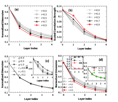
Figure 2: (Color online) Typical behavior of dimension reduction in networks of binary weights. Simulations were carried out on networks of finite size $N=200$, and averaged over ten instances with negligible error bars. (a) Layer-wise dimension reduction with different correlation level $r$. $g=0.9$, $\alpha=2$, and $\sigma_{b}=0.1$. The covariance is obtained by Eq. (1). The cross symbol indicates the simulation result obtained by layer-wise propagating $10^{5}$ samples. (b) Layer-wise decorrelation with $r$. Other parameters are the same as in (a). The neural correlation strength has been scaled by $N$. (c) Dimension reduction and decorrelation with different values of $g$ and $\sigma_{b}$. $r=0.5$. $g=0.9$ when $\sigma_{b}$ varies, and $\sigma_{b}=0.1$ when $g$ varies. (d) Large-$N$ limit behavior for $g=0.4$. The left inset shows the behavior of $\upgamma_{1}$ and the additive term. The right inset shows a comparison of estimated dimensions between theory and simulation ($N=200$). In both insets, $r=0.5$, $\sigma_{b}=0.1$ and $\alpha=2$.

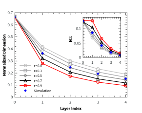
Figure 3: (Color online) Typical behavior of dimension reduction in networks of continuous weights using propagation equation Eq. (1). The results are averaged over ten networks of finite size $N=200$. The error bars are negligible. Simulations indicate layer-wise propagating $10^{5}$ samples. $g=0.9$, $\sigma_{b}=0.1$ and $\alpha=2$.

The elegant way in which the overall neural correlation level is tuned can also be explained by our theory. The weak synaptic correlation contributes an additional additive term in the linear relationship between the input and output neural correlations. This additive term, namely $r^{2}(\mathcal{K}_{1}^{l})^{2}$ [the same for both binary and continuous weights, see Eq. (3) or Eq. (5)], increases the intercept of the linear relationship while maintaining the same slope with the case of $r=0$ (Fig. S1 in [17]). The decorrelation process would thus proceed more slowly when going deeper into the network. The prediction of our theory may then explain the empirical success in improving the classification performance by a deccorrelation regularization of weights [24].

By changing the other statistics of network parameters, say $g$ and $\sigma_{b}$, but fixing $r$, one can observe rich effects of these parameters [Fig. 2 (c)]. First, the dimension reduction seems to be unaffected, or changes by a negligible margin. However, the correlation strength of the hidden representation displays rich behavior. The weight strength elevates the correlation level, as also expected from previous studies [7], playing the similar role to the synaptic correlation [Fig. 2 (b)]. In contrast, increasing the firing bias would further decorrelate the hidden representation. The mechanisms are encoded into Eq. (3) and Eq. (5), in that both the weight strength and firing bias affect the slope and intercept of the linear relationship in a highly non-trivial way, via a recursive iteration from initial values of network activity statistics [17]. These rich effects of tuning the neural correlation of hidden representations may thus shed light on understanding the empirical success of reducing overfitting by optimizing decorrelated representations [25]. The decorrelated representation also coincides with the efficient coding hypothesis in system neuroscience [26]. In this hypothesis, a useful representation should be maximally disentangled, rather than being highly redundant. Our analysis provides a theoretical support for this hypothesis, emphasizing the role of weakly-correlated synapses.

We finally remark that the above analysis also carries over to networks with continuous weights (Fig. 3). Our simulations on deep networks trained with Hebbian learning rules [27, 28] also show key features of the theoretical predictions of our simple model. Details are given in the supplemental material [17].

Summary.—Benefits of weakly-correlated synapses are widely claimed in both system neuroscience [9, 10, 4, 11] and machine learning [24]. The benefits are also realized in a theoretical model of shallow-network unsupervised learning [12], a fundamental process in cerebral cortex [29]. However, the theoretical basis about how weakly-correlated synapses promote the computation in deep neural networks remains unexplored, due to the theoretical complexity of handling the covariance matrix of neural responses. This work tackles the challenge, by deriving mean-field theory for diagonally block-organized correlation matrix of synapses, inspired by our recent work of unsupervised learning [12].

Our work first identifies the unique scaling form of synaptic correlation level, for both binary and continuous weight values, based solely on the mathematical self-consistency. This scaling form may be experimentally testable, like in the intact brain [30]. The theory then reveals in what exact way the weak synaptic correlation tunes both representation dimensionality and associated decorrelation process. More precisely, the synaptic correlation accelerates the dimension reduction, while slowing down the decorrelation process. Both computation roles can be explained in a large-$N$ expansion of our mean-field equations. These predictions coincide with empirical successes in decorrelation regularizations of either synaptic level [24] or neural level [25]. Our theory is thus promising to encourage further understanding of how synaptic and neural correlations interact with each other to yield a disentangled representation supporting the success of deep learning, and even hierarchical information processing in different pathways of neural circuits, a challenging problem in interdisciplinary fields across physics, machine learning and neuroscience [31, 32].

Supplemental Material

Appendix A Theoretical analysis in the large-$N$ limit

In this paper, we consider deep neural networks of either binary or continuous weights. In the case of binary weights, the distribution of $w_{ij}^{l}$ is parametrized by zero mean and the covariance given by

$$\overline{w^{l}_{ij}w^{l}_{ks}}=\delta_{js}{q}+\delta_{ik}\delta_{js}\left(1-{q}\right)={q}\delta_{js}\left(1-\delta_{ik}\right)+\delta_{ik}\delta_{js}\,$$ (S1)

where $\overline{\ \cdot\ }$ denotes the disorder average over the network parameter statistics, and $\delta_{js}$ is the Kronecker delta function. An illustration of this weight covariance is already given in Fig.1 in the main text. For simplicity, we consider only inter-RF correlations, neglecting intra-RF ones. The bias parameter $b_{i}^{l}$ follows independently a Gaussian distribution with zero mean and variance $\sigma_{b}$. The activation $h_{i}^{l}$ is then given by

$$h^{l}_{i}=\phi\left(\frac{g}{\sqrt{N}}\sum_{j}w_{ij}^{l}h^{l-1}_{j}+b^{l}_{i}\right)\ .$$ (S2)

For the continuous-weight case, the parameter $w_{ij}^{l}$ follows the Gaussian distribution with zero mean and the covariance specified by

$$\overline{w^{l}_{ij}w^{l}_{ks}}=\delta_{js}{q}+\delta_{ik}\delta_{js}\left(\frac{g^{2}}{N}-{q}\right)={q}\delta_{js}\left(1-\delta_{ik}\right)+\frac{g^{2}}{N}\delta_{ik}\delta_{js}.$$ (S3)

The bias parameter $b_{i}^{l}$ follows independently a Gaussian distribution with zero mean and variance $\sigma_{b}$. The activation $h_{i}^{l}$ is then given by

$$h^{l}_{i}=\phi\left(\sum_{j}w_{ij}^{l}h^{l-1}_{j}+b^{l}_{i}\right)\ .$$ (S4)

A.1 Mean-field iteration of activity moments

In this section, we derive the mean-field iteration of activity moments. Note that, for both binary and continuous weights, the form of the iteration looks very similar, we here thus derive in detail the iteration for the continuous case. We first derive the mean-field equation for the mean activity $m_{i}^{l}$ as follows,

$$m_{i}^{l} =\langle h_{i}^{l}\rangle$$ (S5)

$$=\left\langle\phi\left(\left[\mathbf{w}^{l}\mathbf{h}^{l-1}\right]_{i}+b_{i}^{l}\right)\right\rangle$$

$$=\left\langle\phi\left(a_{i}^{l}+\left[\mathbf{w}^{l}\mathbf{m}^{l-1}\right]_{i}+b_{i}^{l}\right)\right\rangle\ ,$$

where the average $\left<\cdot\right>$ is defined over the activity statistics throughout the paper, and we define the mean-subtracted weighted-sum (or pre-activation) $a_{i}^{l}=\sum_{j}w_{ij}^{l}\left(h_{j}^{l-1}-\left\langle h_{j}^{l-1}\right\rangle\right)$, then its expectation is zero, and variance is given by $\Delta_{ij}^{l}=\left\langle a_{i}^{l}a_{j}^{l}\right\rangle=\left[\mathbf{w}^{l}\mathbf{C}^{l-1}\left(\mathbf{w}^{l}\right)^{T}\right]_{ij}$, where $\mathbf{C}$ denotes the covariance matrix of the neural activity. Because $a_{i}^{l}$ is the sum of $N$ nearly-independent random terms, as $N\to\infty$, we apply the central limit theorem, and obtain

$$m_{i}^{l} =\int Dt\phi\left(\sqrt{\Delta_{ii}^{l}}t+\sum_{j}w_{ij}^{l}m_{j}^{l-1}+b_{i}^{l}\right)\ ,$$ (S6)

where $Dt=e^{-t^{2}/2}dt/\sqrt{2\pi}$. Then, we consider the covariance of activities. Note that the Gaussian random variable $a_{i}^{l}$ has a variance $\Delta_{ii}^{l}$. The activity covariance is then given by

$$C_{ij}^{l} =\left\langle h_{i}^{l}h_{j}^{l}\right\rangle-\left\langle h_{i}^{l}\right\rangle\left\langle h_{j}^{l}\right\rangle$$ (S7)

$$=\left\langle\phi\left(a_{i}^{l}+\left[\mathbf{w}^{l}\mathbf{m}^{l-1}\right]_{i}+b_{i}^{l}\right)\phi\left(a_{j}^{l}+\left[\mathbf{w}^{l}\mathbf{m}^{l-1}\right]_{j}+b_{j}^{l}\right)\right\rangle-m_{i}^{l}m_{j}^{l}$$

$$=\int DxDy\phi\left(\sqrt{\Delta_{ii}^{l}}x+b_{i}^{l}+\left[\mathbf{w}^{l}\mathbf{m}^{l-1}\right]_{i}\right)\phi\left(\sqrt{\Delta_{jj}^{l}}(\uppsi x+y\sqrt{1-\uppsi^{2}})\right.$$

$$\quad\left.+b_{j}^{l}+\left[\mathbf{w}^{l}\mathbf{m}^{l-1}\right]_{j}\right)-m_{i}^{l}m_{j}^{l}\ ,$$

where $Dx={e^{-x^{2}/2}dx}/{\sqrt{2\pi}}$, and $\uppsi={\Delta_{ij}^{l}}/{\sqrt{\Delta_{ii}^{l}\Delta_{jj}^{l}}}$. $a_{i}^{l}$ and $a_{j}^{l}$ have been parametrized by two independent standard Gaussian random variables, say $x$ and $y$, respectively. The pre-activation correlation has been captured by the correlation coefficient $\uppsi$ ($|\uppsi|\leq 1$).

For binary weights, the above Eqs. (S6), (S7) become

$$m_{i}^{l} =\int Dt\phi\left(\sqrt{\Delta_{ii}^{l}}t+\frac{g}{\sqrt{N}}\sum_{j}w_{ij}^{l}m_{j}^{l-1}+b_{i}^{l}\right)\ ,$$ (S8)

and

$$C_{ij}^{l} =\int DxDy\phi\left(\sqrt{\Delta_{ii}^{l}}x+b_{i}^{l}+\frac{g}{\sqrt{N}}\left[\mathbf{w}^{l}\mathbf{m}^{l-1}\right]_{i}\right)\phi\left(\sqrt{\Delta_{jj}^{l}}(\uppsi x+y\sqrt{1-\uppsi^{2}})\right.$$ (S9)

$$\quad\left.+b_{j}^{l}+\frac{g}{\sqrt{N}}\left[\mathbf{w}^{l}\mathbf{m}^{l1}\right]_{j}\right)-m_{i}^{l}m_{j}^{l}\ ,$$

where

$$\Delta_{ij}^{l}=\frac{g^{2}}{N}\left[\mathbf{w}^{l}\mathbf{C}^{l-1}\left(\mathbf{w}^{l}\right)^{T}\right]_{ij}.$$ (S10)

With the activity moments, we can then evaluate the dimensionality of the $l$-th layer by

$$D^{l}=\frac{\left(\sum_{i}\lambda_{i}\right)^{2}}{\sum_{i}\lambda_{i}^{2}}=\frac{\left(\operatorname{Tr}\mathbf{C}^{l}\right)^{2}}{\operatorname{Tr}(\mathbf{C}^{l})^{2}}=\frac{\left(\sum_{i}C_{ii}^{l}\right)^{2}}{\sum_{i,j}(C_{ij}^{l})^{2}},$$ (S11)

where $\{\lambda_{i}\}$ is the eigen-spectrum of the covariance matrix $\mathbf{C}^{l}$. Then we can define the normalized dimensionality as $\tilde{D}^{l}=\frac{(\operatorname{Tr}\mathbf{C}^{l})^{2}}{N\operatorname{Tr}(\mathbf{C}^{l})^{2}}$, which is then independent of the network width $N$. To derive the recursion of dimensionality for each layer, we define additionally $\mathcal{K}_{1}^{l}=\frac{1}{N}\sum_{i}C_{ii}^{l}$, $\mathcal{K}_{2}^{l}=\frac{1}{N}\sum_{i}(C_{ii}^{l})^{2}$, and $\Upsigma^{l}=\frac{2}{N^{2}}\sum_{i<j}(C_{ij}^{l})^{2}$ for a large value of $N$. The normalized dimensionality of the $l$-th layer is thus expressed as

$$\tilde{D}^{l}=\frac{(\mathcal{K}_{1}^{l})^{2}}{N\Upsigma^{l}+\mathcal{K}_{2}^{l}},$$ (S12)

which is useful for the following theoretical analysis.

A.2 Expansion of two-point correlations

In the mean-field limit, we can assume $C_{ij}^{l}\sim\mathcal{O}(1/\sqrt{N})$ for $i\neq j$ [18]. In the following part, we assume weights take continuous values. Binary weights can be similarly analyzed, by noting that the pre-activations should be multiplied by a pre-factor $g/\sqrt{N}$.

We first analyze the off-diagonal part of the covariance matrix. First, we notice that $\overline{\Delta_{ij}^{2}}=\sum_{k,l}\overline{w_{ik}^{2}}\overline{w_{jl}^{2}}C_{kl}^{2}=N^{2}\frac{g^{2}}{N}\frac{g^{2}}{N}\frac{1}{N}\sim\mathcal{O}\left(\frac{g^{4}}{N}\right)$, which means that $\Delta_{ij}\sim\mathcal{O}(\frac{g^{2}}{\sqrt{N}})$. That is, when $N$ is sufficiently large, $\Delta_{ij}$ is very small. Then we can carry out a Taylor expansion with respect to a small $\Delta_{ij}$ whose layer index is added below:

$$\phi\left(\sqrt{\Delta_{jj}^{l}}(\uppsi x+y\sqrt{1-\uppsi^{2}})+z_{j}^{0}\right) =\phi\left(\sqrt{\Delta_{jj}^{l}}y+z_{j}^{0}\right)$$ (S13)

$$+\phi^{\prime}\left(\sqrt{\Delta_{jj}^{l}}y+z_{j}^{0}\right)\frac{x\Delta_{ij}^{l}}{\sqrt{\Delta_{ii}^{l}}}+\mathcal{O}\left(\left(\Delta_{ij}^{l}\right)^{2}\right),$$

where we define $z_{j}^{0}=b_{j}^{l}+\left[\mathbf{w}^{l}\mathbf{m}^{l-1}\right]_{j}$. By noting that $m_{i}^{l}=\int Dt\phi\left(\sqrt{\Delta_{ii}^{l}}t+z_{i}^{0}\right)$, we obtain

$$C_{ij}^{l} =\int DxDy\phi\left(\sqrt{\Delta_{ii}^{l}}x+z_{i}^{0}\right)\phi^{\prime}\left(\sqrt{\Delta_{jj}^{l}}y+z_{j}^{0}\right)\frac{x\Delta_{ij}^{l}}{\sqrt{\Delta_{ii}^{l}}}+\mathcal{O}\left(\left(\Delta_{ij}^{l}\right)^{2}\right)$$ (S14)

$$=\int DxDy\phi^{\prime}\left(\sqrt{\Delta_{ii}^{l}}x+z_{i}^{0}\right)\phi^{\prime}\left(\sqrt{\Delta^{l}_{jj}}y+z_{j}^{0}\right)\Delta_{ij}^{l}+\mathcal{O}\left(\left(\Delta_{ij}^{l}\right)^{2}\right).$$

Therefore we can write $C_{ij}^{l}\simeq\left<\phi^{\prime}\left(\sqrt{\Delta_{ii}^{l}}x+z_{i}^{0}\right)\right>_{x}\left<\phi^{\prime}\left(\sqrt{\Delta_{jj}^{l}}x+z_{j}^{0}\right)\right>_{y}\Delta_{ij}^{l}$, where the linear coefficient is an average over standard normal variables, and is called hereafter $K_{ij}^{l}$ for the following analysis.

We next remark that $\overline{\Delta_{ii}}\simeq\frac{g^{2}}{N}\sum_{k}\overline{w_{ik}^{2}}C_{kk}=g^{2}\mathcal{K}_{1}\sim\mathcal{O}(g^{2})$. In the small-$g$ limit, we can carry out an expansion in $\sqrt{\Delta_{ii}}$ whose layer index is added below, and get

$$C_{ij}^{l} \simeq\int DxDy\left[\phi^{\prime}\left(z_{i}^{0}\right)+\phi^{\prime\prime}\left(z_{i}^{0}\right)\sqrt{\Delta_{ii}^{l}}x\right]\left[\phi^{\prime}\left(z_{j}^{0}\right)+\phi^{\prime\prime}\left(z_{j}^{0}\right)\sqrt{\Delta^{l}_{jj}}y\right]\Delta_{ij}^{l}$$ (S15)

$$=\phi^{\prime}(z_{i}^{0})\phi^{\prime}(z_{j}^{0})\Delta_{ij}^{l}.$$

This result was reported in our previous work [7]. We then analyze the diagonal part of the covariance matrix,

$$C_{ii}^{l} =\left\langle h_{i}^{l}h_{i}^{l}\right\rangle-\left\langle h_{i}^{l}\right\rangle\left\langle h_{i}^{l}\right\rangle$$ (S16)

$$=\left\langle\phi^{2}\left(a_{i}^{l}+z_{i}^{0}\right)\right\rangle-m_{i}^{l}m_{i}^{l}$$

$$=\int Dx\phi^{2}\left(\sqrt{\Delta_{ii}^{l}}x+z_{i}^{0}\right)-\int Dx\phi\left(\sqrt{\Delta_{ii}^{l}}x+z_{i}^{0}\right)\int Dy\phi\left(\sqrt{\Delta_{ii}^{l}}y+z_{i}^{0}\right).$$

We expand the above formula in the small $\Delta_{ii}^{l}$, i.e., $\phi\left(a_{i}^{l}+z_{i}^{0}\right)=\phi\left(z_{i}^{0}\right)+\phi^{\prime}\left(z_{i}^{0}\right)\sqrt{\Delta_{ii}^{l}}x$, and obtain

$$C_{ii}^{l} \simeq\int Dx\left[\phi\left(z_{i}^{0}\right)+\phi^{\prime}\left(z_{i}^{0}\right)\sqrt{\Delta_{ii}^{l}}x\right]^{2}-\left[\int Dx\left(\phi\left(z_{i}^{0}\right)+\phi^{\prime}\left(z_{i}^{0}\right)\sqrt{\Delta_{ii}^{l}}x\right)\right]^{2}$$ (S17)

$$=\left[\phi^{\prime}(z_{i}^{0})\right]^{2}\Delta_{ii}^{l}.$$

Therefore, we can write $C_{ii}^{l}\simeq K_{ii}^{l}\Delta_{ii}^{l}$, where $K_{ii}^{l}$ is the shorthand for the linear coefficient. To improve the prediction accuracy, one needs to include high-order terms into this approximation. We observe that if we use Eq. (S14) by setting $i=j$, the theoretical prediction in the main text can match the numerical simulation results even in a relatively large value of $g$. This may be due to the fact that the contribution of $\Delta_{ii}^{l}$ is taken into account when computing $K_{ii}^{l}$. For binary weights, the expanded covariance is just the same as the equations [Eq. (S14) and Eq. (S17)], yet with $z_{i}^{0}=b_{i}^{l}+\frac{g}{\sqrt{N}}\left[\mathbf{w}^{l}\mathbf{m}^{l-1}\right]_{i}$.

A.3 Iteration of the correlation strength $\Upsigma^{l}$

A.3.1 Binary weights

First, we calculate $\mathcal{K}_{1}^{l}$, and in the large $N$ and small $g$ limits, we obtain

$$\mathcal{K}_{1}^{l} =\overline{\left(\phi^{\prime}\left(\frac{g}{\sqrt{N}}\sum_{j=1}^{N}w_{ij}^{l}m_{j}^{l-1}+b_{i}^{l}\right)\right)^{2}}\Delta_{ii}^{l}$$ (S18)

$$\simeq\overline{\left(\phi^{\prime}\left(\frac{g}{\sqrt{N}}\sum_{j=1}^{N}w_{ij}^{l}m_{j}^{l-1}+b_{i}^{l}\right)\right)^{2}}g^{2}\mathcal{K}_{1}^{l-1},$$

where $\overline{\ \cdot\ }$ means an average over the distribution of network parameters, and $\Delta_{ii}^{l}$ is approximated by

$$\Delta_{ii}^{l}\simeq\frac{g^{2}}{{N}}\overline{\sum_{k,j}^{N}w_{ik}^{l}w_{ij}^{l}C_{kj}^{l-1}}=\frac{g^{2}}{N}\sum_{k=1}^{N}C_{kk}^{l-1}=g^{2}\mathcal{K}_{1}^{l-1}\ .$$ (S19)

Note that the argument of $\phi^{\prime}(\cdot)$ is a sum of a large number of nearly-independent random variables. It is then easy to write that $\overline{\frac{g}{\sqrt{N}}\sum_{j}w_{ij}^{l}m_{j}^{l-1}+b_{i}^{l}}=0$, and

$$\overline{\left(\frac{g}{\sqrt{N}}\sum_{j}w_{ij}^{l}m_{j}^{l-1}+b_{i}^{l}\right)^{2}}=\frac{g^{2}}{N}\sum_{j}\left(m_{j}^{l-1}\right)^{2}+\sigma_{b}\ .$$

According to the central limit theorem, we obtain

$$\overline{\left(\phi^{\prime}\left(\frac{g}{\sqrt{N}}\sum_{j=1}^{N}w_{ij}^{l}m_{j}^{l-1}+b_{i}^{l}\right)\right)^{2}}=\int Dx\left(\phi^{\prime}(x\sqrt{g^{2}Q^{l-1}+\sigma_{b}})\right)^{2}\stackrel{{\scriptstyle{\rm def}}}{{=}}\overline{K_{ii}^{l}}\ ,$$ (S20)

where we have defined $Q^{l-1}\stackrel{{\scriptstyle{\rm def}}}{{=}}\frac{1}{N}\sum_{i=1}^{N}\left(m_{i}^{l-1}\right)^{2}$. The recursion of $Q^{l}$ becomes

$$Q^{l} =\frac{1}{N}\sum_{i}\left[\int Dt\phi\left(\sqrt{\Delta_{ii}^{l}}t+\frac{g}{\sqrt{N}}\sum_{j}w_{ij}m_{j}^{l-1}+b_{i}^{l}\right)\right]^{2}$$ (S21)

$$=\int Dx\left[\int Dt\phi\Biggl{(}\sqrt{g^{2}\mathcal{K}_{1}^{l-1}}t+x\sqrt{g^{2}Q^{l-1}+\sigma_{b}}\Biggr{)}\right]^{2},$$

where we have used $\Delta_{ii}^{l}=g^{2}\mathcal{K}_{1}^{l-1}$.

Finally, we obtain the recursion for $\mathcal{K}_{1}^{l}$,

$$\mathcal{K}_{1}^{l}=g^{2}\overline{K_{ii}^{l}}\mathcal{K}_{1}^{l-1}.$$ (S22)

Note that $\mathcal{K}_{1}^{l}$ can also be calculated recursively without the small-$g$ assumption as follows,

$$\mathcal{K}_{1}^{l} =\int DxDt\phi^{2}\left(\sqrt{g^{2}\mathcal{K}_{1}^{l-1}}t+x\sqrt{\sigma_{b}+g^{2}Q^{l-1}}\right)-Q^{l}$$ (S23)

$$=\int Dx\phi^{2}\left(\sqrt{g^{2}\mathcal{K}_{1}^{l-1}+\sigma_{b}+g^{2}Q^{l-1}}\ x\right)-Q^{l}.$$

Next, the recursion of $\mathcal{K}_{2}^{l}$ can be calculated by definition as follows,

$$\mathcal{K}_{2}^{l} =\frac{1}{N}\sum_{i}\left(C_{ii}^{l}\right)^{2}$$ (S24)

$$=\frac{1}{N}\sum_{i}\left(K_{ii}^{l}g^{2}\mathcal{K}_{1}^{l-1}\right)^{2}$$

$$=\overline{(K_{ii}^{l})^{2}}g^{4}(\mathcal{K}_{1}^{l-1})^{2}\ ,$$

where we have assumed that $K_{ii}^{l}$ in the large-$N$ limit does not depend on the specific site index, and thus

$$\overline{(K_{ii}^{l})^{2}}=\overline{\left(\phi^{\prime}\left(\frac{g}{\sqrt{N}}\sum_{j}w_{ij}^{l}m_{j}^{l-1}+b_{i}^{l}\right)\right)^{4}}=\int Dx\left(\phi^{\prime}(x\sqrt{g^{2}Q^{l-1}+\sigma_{b}})\right)^{4}\ .$$ (S25)

Note that $\mathcal{K}_{2}^{l}$ can be evaluated recursively without the small-$g$ assumption as

$$\mathcal{K}_{2}^{l}=\left<\left[\left<\phi^{2}(f)\right>_{z}-\left<\phi(f)\right>_{z}^{2}\right]^{2}\right>_{u,t},$$ (S26)

where $z$, $u$, and $t$ are all standard normal variables, and $f\stackrel{{\scriptstyle{\rm def}}}{{=}}\sqrt{g^{2}\mathcal{K}_{1}^{l-1}}z+\sqrt{\sigma_{b}}u+\sqrt{g^{2}Q^{l-1}}t$.

We finally derive the recursion of $\Upsigma^{l}$. First, for the binary weights, to compute $\Delta_{ij}^{2}$, where the layer index can be added later, we have

$$\left(\sum_{k,l}w_{ik}w_{jl}C_{kl}\right)^{2} =\left(\sum_{k\neq l}w_{ik}w_{jl}C_{kl}+\sum_{k}w_{ik}w_{jk}C_{kk}\right)^{2}$$ (S27)

$$\simeq\sum_{k\neq l;k^{\prime}\neq l^{\prime}}w_{ik}w_{ik^{\prime}}w_{jl}w_{jl^{\prime}}C_{kl}C_{k^{\prime}l^{\prime}}+\sum_{k,k^{\prime}}w_{ik}w_{jk}w_{ik^{\prime}}w_{jk^{\prime}}C_{kk}C_{k^{\prime}k^{\prime}}$$

$$\simeq(1+q^{2})\sum_{k\neq l}C_{kl}^{2}+(1-q^{2})\sum_{k}C_{kk}^{2}+q^{2}\left(\sum_{k}C_{kk}\right)^{2},$$

where the cross-term vanishes in statistics to derive the second equality, due to the vanishing intra-RF correlation for one hidden neuron. The third equality is derived by considering the inter-RF correlation in our current setting. Finally, we arrive at

$$N\Upsigma^{l+1} =\frac{2}{N}\sum_{i<j}\overline{(K_{ij}^{l+1})^{2}}\frac{g^{4}}{N^{2}}\left[(1+q^{2})N^{2}\Upsigma^{l}+(1-q^{2})N\mathcal{K}_{2}^{l}+q^{2}N^{2}\left(\mathcal{K}_{1}^{l}\right)^{2}\right]$$ (S28)

$$=\overline{(K_{ij}^{l+1})^{2}}g^{4}\left[(1+q^{2})N\Upsigma^{l}+q^{2}N(\mathcal{K}_{1}^{l})^{2}+(1-q^{2})\mathcal{K}_{2}^{l}\right]$$

$$\simeq\overline{(K_{ij}^{l+1})^{2}}g^{4}\left[N\Upsigma^{l}+\mathcal{K}_{2}^{l}+r^{2}(\mathcal{K}_{1}^{l})^{2}\right]\ ,$$

where we have to assume $q=r/\sqrt{N}$ [$r\sim\mathcal{O}(1)$], and $\overline{(K_{ij}^{l+1})^{2}}$ is used to replace $(K_{ij}^{l+1})^{2}$ in the mean-field approximation and can be computed recursively as follows,

$$\overline{(K_{ij}^{l+1})^{2}} =\left<\left<\phi^{\prime}\left(\sqrt{g^{2}\mathcal{K}_{1}^{l}}x+\sqrt{g^{2}Q^{l}}z_{1}+\sqrt{\sigma_{b}}u_{1}\right)\right>^{2}_{x}\right.$$ (S29)

$$\left.\times\left<\phi^{\prime}\left(\sqrt{g^{2}\mathcal{K}_{1}^{l}}y+\sqrt{g^{2}Q^{l}}\left(\rho z_{1}+\sqrt{1-\rho^{2}}z_{2}\right)+\sqrt{\sigma_{b}}u_{2}\right)\right>^{2}_{y}\right>_{z_{1},z_{2},u_{1},u_{2}},$$

where $x,y,z_{1},z_{2},u_{1},u_{2}$ are all standard Gaussian random variables, capturing both thermal and disorder average (inner and outer ones respectively). The correlation coefficient is given by

$$\rho\stackrel{{\scriptstyle{\rm def}}}{{=}}\frac{\overline{(z_{i}^{0}-b_{i})(z_{j}^{0}-b_{j})}}{\sqrt{\overline{(z_{i}^{0}-b_{i})^{2}}\cdot\overline{(z_{j}^{0}-b_{j})^{2}}}}=q.$$ (S30)

Therefore, $q$ plays an important role in our current theory, in contrast to the orthogonal case [7].

A.3.2 Continuous weights

First, we calculate $\mathcal{K}_{1}^{l}$, and in the large $N$ limit, we obtain

$$\mathcal{K}_{1}^{l} =\overline{\left(\phi^{\prime}\left(\sum_{j}w_{ij}^{l}m_{j}^{l-1}+b_{i}^{l}\right)\right)^{2}}\Delta_{ii}^{l}$$ (S31)

$$\simeq\overline{\left(\phi^{\prime}\left(\sum_{j}w_{ij}^{l}m_{j}^{l-1}+b_{i}^{l}\right)\right)^{2}}g^{2}\mathcal{K}_{1}^{l-1},$$

where $\overline{\ \cdot\ }$ means an average over the distribution of network parameters, and $\Delta_{ii}^{l}$ can be approximated by

$$\Delta_{ii}^{l}\simeq\overline{\sum_{k,j}^{N}w_{ik}^{l}w_{ij}^{l}C_{kj}^{l-1}}=\frac{g^{2}}{N}\sum_{k=1}^{N}C_{kk}^{l-1}=g^{2}\mathcal{K}_{1}^{l-1}\ .$$ (S32)

The argument of $\phi^{\prime}(\cdot)$ is a sum of a large number of nearly-independent random variables, as a result, it is easy to write that $\overline{\sum_{j}w_{ij}^{l}m_{j}^{l-1}+b_{i}^{l}}=0$, and

$$\overline{\left(\sum_{j}w_{ij}^{l}m_{j}^{l-1}+b_{i}^{l}\right)^{2}}=\frac{g}{N}\sum_{j}\left(m_{j}^{l-1}\right)^{2}+\sigma_{b}\ .$$

According to the central limit theorem, we obtain

$$\overline{\left(\phi^{\prime}\left(\sum_{j=1}^{N}w_{ij}^{l}m_{j}^{l-1}+b_{i}^{l}\right)\right)^{2}}=\int Dx\left(\phi^{\prime}(x\sqrt{g^{2}Q^{l-1}+\sigma_{b}})\right)^{2}\stackrel{{\scriptstyle{\rm def}}}{{=}}\overline{K_{ii}^{l}}\ ,$$ (S33)

where we have defined $Q^{l-1}\stackrel{{\scriptstyle{\rm def}}}{{=}}\frac{1}{N}\sum_{i}\left(m_{i}^{l-1}\right)^{2}$. The recursion of $Q^{l}$ becomes

$$Q^{l} =\frac{1}{N}\sum_{i}\left[\int Dt\phi\left(\sqrt{\Delta_{ii}^{l}}t+\sum_{j}w_{ij}m_{j}^{l-1}+b_{i}^{l}\right)\right]^{2}$$ (S34)

$$=\int Dx\left[\int Dt\phi\Biggl{(}\sqrt{g^{2}\mathcal{K}_{1}^{l-1}}t+x\sqrt{g^{2}Q^{l-1}+\sigma_{b}}\Biggr{)}\right]^{2},$$

where we have used $\Delta_{ii}^{l}=g^{2}\mathcal{K}_{1}^{l-1}$.

Finally, we obtain the recursion for $\mathcal{K}_{1}^{l}$ as

$$\mathcal{K}_{1}^{l}=g^{2}\overline{K_{ii}^{l}}\mathcal{K}_{1}^{l-1}.$$ (S35)

Note that $\mathcal{K}_{1}^{l}$ can also be calculated recursively without the small-$g$ assumption as follows,

$$\mathcal{K}_{1}^{l}=\int Dx\phi^{2}\left(\sqrt{g^{2}\mathcal{K}_{1}^{l-1}+\sigma_{b}+g^{2}Q^{l-1}}\ x\right)-Q^{l}.$$ (S36)

We then derive $\mathcal{K}_{2}^{l}$ as follows,

$$\mathcal{K}_{2}^{l} =\frac{1}{N}\sum_{i}\left(C_{ii}^{l}\right)^{2}$$ (S37)

$$=\frac{1}{N}\sum_{i}\left(K_{ii}^{l}g^{2}\mathcal{K}_{1}^{l-1}\right)^{2}$$

$$=\overline{(K_{ii}^{l})^{2}}g^{4}(\mathcal{K}_{1}^{l-1})^{2}\ ,$$

where $(K_{ii}^{l})^{2}$ is approximated by

$$\overline{(K_{ii}^{l})^{2}}=\overline{\left(\phi^{\prime}\left(\sum_{j}w_{ij}^{l}m_{j}^{l-1}+b_{i}^{l}\right)\right)^{4}}=\int Dx\left(\phi^{\prime}(x\sqrt{g^{2}Q^{l-1}+\sigma_{b}})\right)^{4}\ .$$ (S38)

Note that $\mathcal{K}_{2}^{l}$ can be evaluated recursively without the small-$g$ assumption as

$$\mathcal{K}_{2}^{l}=\left<\left[\left<\phi^{2}(f)\right>_{z}-\left<\phi(f)\right>_{z}^{2}\right]^{2}\right>_{u,t},$$ (S39)

where $z$, $u$, and $t$ are all standard normal variables, and $f\stackrel{{\scriptstyle{\rm def}}}{{=}}\sqrt{g^{2}\mathcal{K}_{1}^{l-1}}z+\sqrt{\sigma_{b}}u+\sqrt{g^{2}Q^{l-1}}t$.

To finally obtain the recursion of $\Upsigma^{l}$, we first analyze $\Delta_{ij}^{2}$ whose layer index will be added later as follows,

$$\Delta_{ij}^{2} =\left(\sum_{k,l}w_{ik}w_{jl}C_{kl}\right)^{2}=\left(\sum_{k\neq l}w_{ik}w_{jl}C_{kl}+\sum_{k}w_{ik}w_{jk}C_{kk}\right)^{2}$$ (S40)

$$\simeq\sum_{k\neq l;k^{\prime}\neq l^{\prime}}w_{ik}w_{ik^{\prime}}w_{jl}w_{jl^{\prime}}C_{kl}C_{k^{\prime}l^{\prime}}+\sum_{k,k^{\prime}}w_{ik}w_{jk}w_{ik^{\prime}}w_{jk^{\prime}}C_{kk}C_{k^{\prime}k^{\prime}}$$

$$\simeq\left(\frac{g^{4}}{N^{2}}+q^{2}\right)\sum_{k\neq l}C_{kl}^{2}+\frac{g^{4}}{N^{2}}(2\rho^{2}+1)\sum_{k}C_{kk}^{2}$$

$$+q^{2}\left[\left(\sum_{k}C_{kk}\right)^{2}-\sum_{k}C_{kk}^{2}\right],$$

where $\rho=\frac{qN}{g^{2}}$ due to the fact that $\overline{w_{ik}w_{jk}}=q$ as well as $\overline{w_{ik}^{2}}=g^{2}/N$. To arrive at the final equality, we have used the statistics equality as follows,

$$\overline{w_{ik}^{2}w_{jk}^{2}} =\left<\frac{g^{2}}{N}z_{1}^{2}\times\frac{g^{2}}{N}(\rho z_{1}+\sqrt{1-\rho^{2}}z_{2})^{2}\right>_{z_{1},z_{2}\sim\mathcal{N}(0,1)}$$ (S41)

$$=\frac{g^{4}}{N^{2}}(2\rho^{2}+1).$$

We finally arrive at the recursion for $\Upsigma^{l}$ as follows,

$$N\Upsigma^{l} \simeq\frac{2}{N}\sum_{i<j}\overline{(K_{ij}^{l})^{2}}\left[\left(\frac{g^{4}}{N^{2}}+q^{2}\right)\sum_{k\neq j}(C_{kj}^{l-1})^{2}+\left(q^{2}+\frac{g^{4}}{N^{2}}\right)\sum_{k}(C_{kk}^{l-1})^{2}+q^{2}\left(\sum_{k}C_{kk}^{l-1}\right)^{2}\right]$$ (S42)

$$=\overline{(K_{ij}^{l})^{2}}\left[(g^{4}+N^{2}q^{2})(N\Upsigma^{l-1}+\mathcal{K}_{2}^{l-1})+q^{2}N^{3}(\mathcal{K}_{1}^{l-1})^{2}\right]$$

$$=\overline{(K_{ij}^{l})^{2}}\left[g^{4}(N\Upsigma^{l-1}+\mathcal{K}_{2}^{l-1})+r^{2}(\mathcal{K}_{1}^{l-1})^{2}\right]\ ,$$

where we have to assume $q=r/N^{\frac{3}{2}}$ [$r\sim\mathcal{O}(1)$], and $\overline{(K_{ij}^{l})^{2}}$ is used to approximate $(K_{ij}^{l})^{2}$ and can be computed as follows,

$$\overline{(K_{ij}^{l})^{2}} =\left<\left<\phi^{\prime}\left(\sqrt{g^{2}\mathcal{K}_{1}^{l-1}}x+\sqrt{g^{2}Q^{l-1}}z_{1}+\sqrt{\sigma_{b}}u_{1}\right)\right>^{2}_{x}\right.$$ (S43)

$$\left.\times\left<\phi^{\prime}\left(\sqrt{g^{2}\mathcal{K}_{1}^{l-1}}y+\sqrt{g^{2}Q^{l-1}}\left(\rho z_{1}+\sqrt{1-\rho^{2}}z_{2}\right)+\sqrt{\sigma_{b}}u_{2}\right)\right>^{2}_{y}\right>_{z_{1},z_{2},u_{1},u_{2}},$$

where $x,y,z_{1},z_{2},u_{1},u_{2}$ are all standard Gaussian random variables, capturing both thermal and disorder average (inner and outer ones respectively). The correlation coefficient in the continuous-weight case is given by

$$\rho\stackrel{{\scriptstyle{\rm def}}}{{=}}\frac{\overline{(z_{i}^{0}-b_{i})(z_{j}^{0}-b_{j})}}{\sqrt{\overline{(z_{i}^{0}-b_{i})^{2}}\cdot\overline{(z_{j}^{0}-b_{j})^{2}}}}=\frac{qN}{g^{2}}.$$ (S44)

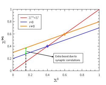
Figure S1: The schematic illustration showing how synaptic correlations elevate the neural correlation level (multiplied by $N$) and the operating point in hidden representations of deep neural networks. The boost is indicated by the double arrow for an example in which the input $\Upsigma^{l}$ is below the operating point (indicated by star-symbols) where $\Upsigma^{l+1}=\Upsigma^{l}$.

We finally remark that the synaptic correlation is able to boost the neural correlation level when transmitting signal via hidden representations. From the linear relationship between $\Upsigma^{l+1}$ and $\Upsigma^{l}$ [see Eq. (S28)], one derives for the binary weights that the operating point is given by:

$$\Upsigma_{*}^{l}=\frac{\Upsilon\mathcal{K}_{2}^{l}}{1-\Upsilon}+\frac{\Upsilon r^{2}(\mathcal{K}_{1}^{l})^{2}}{1-\Upsilon},$$ (S45)

where $\Upsigma_{*}^{l}$ has been multiplied by $N$, and $\Upsilon\stackrel{{\scriptstyle{\rm def}}}{{=}}g^{4}\overline{(K_{ij}^{l+1})^{2}}$. Eq. (S45) implies that the operating point is increased by the synaptic correlations (the last term in the equation). The intercept of the linear relationship is also increased by a positive amount $\Upsilon r^{2}(\mathcal{K}_{1}^{l})^{2}$. Note that the slope of the linear relationship under the orthogonal-weight and correlated-weight cases are the same. These effects are qualitatively the same for both continuous and binary weights, which is shown in Fig. S1.

A.4 Iteration of the dimensionality across layers

A.4.1 Binary weights

According to the definition, with the help of Eqs. (S22) and (S24) and the recursion equation for $\Upsigma^{l}$, we obtain

$$\tilde{D}^{l} =\frac{\left(\mathcal{K}_{1}^{l}\right)^{2}}{N\Upsigma^{l}+\mathcal{K}_{2}^{l}}$$ (S46)

$$=\frac{(\mathcal{K}_{1}^{l-1})^{2}}{\upgamma_{1}(N\Upsigma^{l-1}+\mathcal{K}_{2}^{l-1})+\left(\upgamma_{1}{r^{2}}+\upgamma_{2}\right)\left(\mathcal{K}_{1}^{l-1}\right)^{2}}\ ,$$

where $\upgamma_{1}=\overline{K_{ij}^{2}}/{\overline{K_{ii}}^{2}}$, $\upgamma_{2}=\overline{K_{ii}^{2}}/\overline{K_{ii}}^{2}$ and $r=qN^{\frac{1}{2}}$. When the superscripts of layer index for $K_{ij}$ and $K_{ii}$ are clear, the superscripts are omitted. Here, we manage to use the activity statistics at previous layers to estimate the dimensionality of the current layer, rather than the original formula [Eq. (S12)]. Thus the mechanism for dimensionality change can be revealed.

Note that to evaluate $\upgamma_{1}$ and $\upgamma_{2}$, we need to compute the following quantities,

$$\overline{K_{ii}} =\left<\left(\phi^{\prime}\left(x\sqrt{g^{2}Q^{l-1}+\sigma_{b}}\right)\right)^{2}\right>_{x}\ ,$$ (S47)

$$\overline{K_{ii}^{2}} =\left<\left(\phi^{\prime}\left(y\sqrt{g^{2}Q^{l-1}+\sigma_{b}}\right)\right)^{4}\right>_{y}\ ,$$

$$\overline{K_{ij}^{2}} =\left<\left<\phi^{\prime}\left(\sqrt{g^{2}\mathcal{K}_{1}^{l-1}}x+\sqrt{g^{2}Q^{l-1}}z_{1}+\sqrt{\sigma_{b}}u_{1}\right)\right>^{2}_{x}\right.$$

$$\left.\times\left<\phi^{\prime}\left(\sqrt{g^{2}\mathcal{K}_{1}^{l-1}}y+\sqrt{g^{2}Q^{l-1}}\left(\rho z_{1}+\sqrt{1-\rho^{2}}z_{2}\right)+\sqrt{\sigma_{b}}u_{2}\right)\right>^{2}_{y}\right>_{z_{1},z_{2},u_{1},u_{2}}\ ,$$

where $\rho=q$. $Q^{l}$, $\mathcal{K}_{1}^{l}$, and $\mathcal{K}_{2}^{l}$ can also be computed recursively by following the iterative equations in Sec. A.3.1.

A.4.2 Continuous weights

According to the definition, with the help of Eqs. (S35) and (S37) and the recursion equation for $\Upsigma^{l}$, we obtain

$$\tilde{D}^{l} =\frac{\left(\mathcal{K}_{1}^{l}\right)^{2}}{N\Upsigma^{l}+\mathcal{K}_{2}^{l}}$$ (S48)

$$=\frac{\overline{K_{ii}}^{2}g^{4}(\mathcal{K}_{1}^{l-1})^{2}}{\overline{K_{ij}^{2}}\left(g^{4}(N\Upsigma^{l-1}+\mathcal{K}_{2}^{l-1})+r^{2}(\mathcal{K}_{1}^{l-1})^{2}\right)+\overline{K_{ii}^{2}}g^{4}(\mathcal{K}_{1}^{l-1})^{2}}$$

$$=\frac{(\mathcal{K}_{1}^{l-1})^{2}}{\upgamma_{1}(N\Upsigma^{l-1}+\mathcal{K}_{2}^{l-1})+\left(\upgamma_{1}\frac{r^{2}}{g^{4}}+\upgamma_{2}\right)\left(\mathcal{K}_{1}^{l-1}\right)^{2}}\ ,$$

where $\upgamma_{1}=\overline{K_{ij}^{2}}/{\overline{K_{ii}}^{2}}$, $\upgamma_{2}=\overline{K_{ii}^{2}}/\overline{K_{ii}}^{2}$ and $r=qN^{\frac{3}{2}}$. When the superscripts of layer index for $K_{ij}$ and $K_{ii}$ are clear, the superscripts are omitted. The iterative equations for computing $\upgamma_{1}$ and $\upgamma_{2}$ are the same with Eq. (S47), yet with $\rho=\frac{qN}{g^{2}}$ for the continuous-weight case. $Q^{l}$, $\mathcal{K}_{1}^{l}$, and $\mathcal{K}_{2}^{l}$ can also be computed recursively by following the iterative equations in Sec. A.3.2.

A.5 Closed-form mean-field iterations for estimating the dimensionality

For continuous weights, the mean-field iteration of the covariance matrix of activations is given by

$$\Delta^{l}_{ij}=\sum_{k,k^{\prime}}w^{l}_{ik}C^{l-1}_{kk^{\prime}}w^{l}_{jk^{\prime}},$$ (S49)

$$m_{i}^{l} =\int Dt\phi\left(\sqrt{\Delta_{ii}^{l}}t+\sum_{j=1}^{N}w_{ij}^{l}m_{j}^{l-1}+b_{i}^{l}\right)\ ,$$ (S50)

and

$$C_{ij}^{l} =\int DxDy\phi\left(\sqrt{\Delta_{ii}^{l}}x+b_{i}^{l}+\sum_{k}{w}^{l}_{ik}{m}^{l-1}_{k}\right)\times$$ (S51)

$$\quad\phi\left(\sqrt{\Delta_{jj}^{l}}(\uppsi x+y\sqrt{1-\uppsi^{2}})+b_{j}^{l}+\sum_{k^{\prime}}{w}^{l}_{jk^{\prime}}{m}^{l-1}_{k^{\prime}}\right)-m_{i}^{l}m_{j}^{l}\ ,$$

where $Dx={e^{-x^{2}/2}dx}/{\sqrt{2\pi}}$, and $\uppsi={\Delta_{ij}^{l}}/{\sqrt{\Delta_{ii}^{l}\Delta_{jj}^{l}}}$. By taking the covariance matrix $\Lambda$ and zero mean of the data as initial values, we can get the covariance matrix of the activation values of each subsequent layer by iterating the above mean-field equations [Eqs. (S49), (S50), and (S51)]. Then according to the formula $D=\left(\operatorname{Tr}\mathbf{C}\right)^{2}/\operatorname{Tr}\mathbf{C}^{2}$, the representation dimensionality of each layer can be calculated.

For binary weights, the equation of the mean-field iteration is just a bit different, given by

$$\Delta_{ij}^{l}=\frac{g^{2}}{N}\sum_{k,k^{\prime}}w^{l}_{ik}C^{l-1}_{kk^{\prime}}w^{l}_{jk^{\prime}},$$ (S52)

$$m_{i}^{l} =\int Dt\phi\left(\sqrt{\Delta_{ii}^{l}}t+\frac{g}{\sqrt{N}}\sum_{j=1}^{N}w_{ij}^{l}m_{j}^{l-1}+b_{i}^{l}\right)\ ,$$ (S53)

and

$$C_{ij}^{l} =\int DxDy\phi\left(\sqrt{\Delta_{ii}^{l}}x+b_{i}^{l}+\frac{g}{\sqrt{N}}\sum_{k}w_{ik}^{l}m_{k}^{l-1}\right)\cdot$$ (S54)

$$\quad\phi\left(\sqrt{\Delta_{jj}^{l}}(\uppsi x+y\sqrt{1-\uppsi^{2}})+b_{j}^{l}+\frac{g}{\sqrt{N}}\sum_{k^{\prime}}w_{jk^{\prime}}^{l}m_{k^{\prime}}^{l-1}\right)-m_{i}^{l}m_{j}^{l}\ .$$

The procedure of estimating the linear dimensionality is similar to that of the continuous-weight case.

Appendix B Numerical generation of weight-correlated neural networks

We consider a five-layer fully connected neural network with one input layer and four hidden layers. The number of neurons in each layer is specified by $N$. The parameters of the network are generated by following the procedure below, and after the initialization, all parameters remain unchanged during the simulation of dimension estimation, and then the result is averaged over many independent realizations of the same statistics of network parameters.

B.1 Binary weights

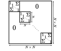
Figure S2: The schematic illustration of the covariance matrix of ${\bm{x}}^{l}$ used to generate correlated binary weights.

The binary weight ($w_{ij}=\pm 1$) follows a statistics of zero mean and the covariance specified by

$$\overline{w^{l}_{ij}w^{l}_{ks}}=\delta_{js}{q}+\delta_{ik}\delta_{js}\left(1-{q}\right)={q}\delta_{js}\left(1-\delta_{ik}\right)+\delta_{ik}\delta_{js}\ .$$ (S55)

Diagonalization of the full covariance matrix of binary weights is challenging. However, no correlation occurs within each RF. Then we can generate the network weights for each diagonal block in Fig.1 (see the main text) independently by a dichotomized Gaussian (DG) process [33]. In the DG process, the binary weights can be generated by $w_{ij}^{l}=\operatorname{sign}(x^{l}_{ij})$, where

$$\operatorname{sign}(x)=\begin{cases}1&x\geq 0\\ -1&x<0\end{cases},$$ (S56)

where $x^{l}_{ij}$ is sampled from a multivariate Gaussian distribution of zero mean (due to $\overline{w_{ij}^{l}}=0$) and the following covariance, as also shown in a schematic illustration in Fig. S2,

$$\overline{x^{l}_{ij}x^{l}_{ks}}=\delta_{js}{\Sigma}+\delta_{ik}\delta_{js}\left(1-{\Sigma}\right)={\Sigma}\delta_{js}\left(1-\delta_{ik}\right)+\delta_{ik}\delta_{js}\ .$$ (S57)

The relation between $q$ and $\Sigma$ can be established by matching the covariance of the DG process with our prescribed correlation level $q$, i.e.,

$$q=\iint DxDy\operatorname{sign}(x)\operatorname{sign}\left(\Sigma x+\sqrt{1-\Sigma^{2}}y\right)=\frac{2}{\pi}\arcsin\Sigma.$$ (S58)

Then, we have

$$\Sigma=\sin\frac{\pi q}{2}.$$ (S59)

A sample of the multivariate Gaussian distribution with the $N\times N$ covariance matrix $\bm{\Sigma}$ (diagonal blocks in Fig. S2) can be obtained by first carrying out a Cholesky decomposition of the covariance, i.e., $\bm{\Sigma}=\mathbf{L}\mathbf{L}^{{\rm T}}$, where $\mathbf{L}$ is a lower-triangular matrix. A sample is then obtained as $\mathbf{z}=\mathbf{L}\bm{\epsilon}$, where $\bm{\epsilon}\sim\mathcal{N}(\mathbf{0},\mathbbm{I})$. $\mathbbm{I}$ denotes an identity matrix. The parameter $b_{i}^{l}$ follows $\mathcal{N}(0,\sigma_{b})$ independently.

B.2 Continuous weights

For the continuous case, the parameter $w_{ij}^{l}$ follows the Gaussian distribution with zero means and the covariance specified by

$$\overline{w^{l}_{ij}w^{l}_{ks}}=\delta_{js}{q}+\delta_{ik}\delta_{js}\left(\frac{g^{2}}{N}-{q}\right)={q}\delta_{js}\left(1-\delta_{ik}\right)+\frac{g^{2}}{N}\delta_{ik}\delta_{js}.$$ (S60)

When generating the weights, we divide $\mathbf{w}^{l}$ into $N$ vectors, each of which is defined by $[w_{1j}^{l},$ $w_{2j}^{l},\cdots,w_{Nj}^{l}]$ ($j=1,2,\cdots,N$). Then all those vectors are independently sampled from a multivariate Gaussian distribution with zero means and the covariance matrix $\bm{\Sigma}\in\mathbb{R}^{N\times N}$, in which $\bm{\Sigma}$ is a symmetric matrix with diagonal elements $g^{2}/N$ and off-diagonal elements $q$. The parameter $b_{i}^{l}$ follows $\mathcal{N}(0,\sigma_{b})$ independently.

Appendix C Numerical generation of input data samples following the pre-defined covariance

The input dataset for our deep transformation include $100000$ data samples, which are independently sampled from a multivariate Gaussian distribution with zero means and the covariance matrix specified by $\Lambda=\frac{1}{N}\bm{\xi}\bm{\xi}^{{\rm T}}$, where $\bm{\xi}\in\mathbb{R}^{N\times P}$ and its elements follow a Gaussian distribution $\xi_{ij}\sim\mathcal{N}(0,\sigma^{2})$. We define $\alpha=P/N$, and the relation between $\alpha$ and $\tilde{D}$ can be proved to be $\tilde{D}=\alpha/(1+\alpha)$, as we shall show later.

First, we need to calculate the eigenvalue spectrum of $\Lambda$, namely $\{\lambda_{i}^{\Lambda}\}$ by replica trick [34]. The Edwards-Jones formula reads

$$\rho(\lambda) =\frac{1}{N}\sum_{i=1}^{N}\delta(\lambda-\lambda_{i}^{\Lambda})$$ (S61)

$$=\frac{1}{N\pi}\lim_{\epsilon\rightarrow 0^{+}}\operatorname{Im}\frac{\partial}{\partial\lambda}\left<\ln\operatorname{det}(\lambda_{\epsilon}\mathbbm{I}-\Lambda)\right>_{\Lambda}$$

$$=\frac{-2}{\pi N}\lim_{\epsilon\rightarrow 0^{+}}\operatorname{Im}\frac{\partial}{\partial\lambda}\langle\ln Z(\lambda)\rangle_{\Lambda}\ ,$$

where the Sokhotski-Plemelj identity is used to derive the second equality, and a Gaussian integral representation of the determinant leads to

$$Z(\lambda)=\int_{\mathbb{R}^{N}}d\bm{y}\exp\left[-\frac{1}{2}\bm{y}^{T}\left(\lambda_{\epsilon}\mathbb{I}-\Lambda\right)\bm{y}\right]\ ,$$ (S62)

where $\lambda_{\epsilon}=\lambda-\mathrm{i}\epsilon$, and $d\bm{y}\stackrel{{\scriptstyle{\rm def}}}{{=}}\prod_{i}\frac{dy_{i}}{\sqrt{2\pi}}$.

Hereafter, for simplicity, we consider only the annealed average $\langle Z(\lambda)\rangle_{\Lambda}$, instead of the more complex quenched one like that analyzed in Ref. [34]. The result will be cross-checked by numerical experiments. In some cases, the annealed average agrees with the quenched one via replica trick, due to the fact that different replicas of the Gaussian variables $\bm{y}$ are decoupled [35]. It then proceeds as follows,

$$\langle Z(\lambda)\rangle =\int d\bm{y}\left\langle\exp\left[-\frac{1}{2}\bm{y}^{T}\left(\lambda_{\epsilon}\mathbb{I}-\Lambda\right)\bm{y}\right]\right\rangle$$ (S63)

$$=\int d\bm{y}\exp\left[-\frac{1}{2}\lambda_{\epsilon}\bm{y}^{T}\bm{y}\right]\left\langle\exp\left[\frac{1}{2N}\bm{y}^{T}\bm{\xi}\bm{\xi}^{T}\bm{y}\right]\right\rangle$$

$$=\int d\bm{y}\exp\left[-\frac{1}{2}\lambda_{\epsilon}\sum_{i=1}^{N}y_{i}^{2}\right]\left\langle\exp\left[\frac{1}{2N}\sum_{j=1}^{P}\left(\sum_{i=1}^{N}y_{i}\xi_{ij}\right)^{2}\right]\right\rangle$$

$$=\int d\bm{y}\exp\left[-\frac{1}{2}\lambda_{\epsilon}\sum_{i=1}^{N}y_{i}^{2}\right]\left\langle\prod_{j=1}^{P}\exp\left[\frac{1}{2N}\left(\sum_{i=1}^{N}y_{i}\xi_{ij}\right)^{2}\right]\right\rangle$$

$$\propto\int d\bm{y}d\bm{m}\exp\left[-\frac{1}{2}\lambda_{\epsilon}\sum_{i=1}^{N}y_{i}^{2}-\sum_{j=1}^{P}m_{j}^{2}\right]\left\langle\prod_{j=1}^{P}\prod_{i=1}^{N}\exp\left[2\sqrt{\frac{1}{2N}}m_{j}y_{i}\xi_{ij}\right]\right\rangle\,,$$

where $d\bm{m}\stackrel{{\scriptstyle{\rm def}}}{{=}}\prod_{i}\frac{dm_{i}}{\sqrt{\pi}}$, and we have used the integral identity for $\bm{m}$:

$$e^{b^{2}}=\frac{1}{\sqrt{\pi}}\int e^{-x^{2}+2bx}dx.$$ (S64)

We then calculate the expectation with respect to $\bm{\xi}$, and obtain

$$\left\langle\prod_{j=1}^{P}\prod_{i=1}^{N}\exp\left[2\sqrt{\frac{1}{2N}}m_{j}y_{i}\xi_{ij}\right]\right\rangle_{\bm{\xi}} =\prod_{j=1}^{P}\prod_{i=1}^{N}\left\langle\exp\left[2\sqrt{\frac{1}{2N}}m_{j}y_{i}\xi_{ij}\right]\right\rangle_{\xi_{ij}}$$ (S65)

$$=\prod_{j=1}^{P}\prod_{i=1}^{N}\exp\left[{\frac{1}{N}}\sigma^{2}m_{j}^{2}y_{i}^{2}\right].$$

Thus,

$$\langle Z(\lambda)\rangle \propto\int d\bm{y}d\bm{m}\exp\left[-\frac{1}{2}\lambda_{\epsilon}\sum_{i=1}^{N}y_{i}^{2}-\sum_{j=1}^{P}m_{j}^{2}+{\frac{1}{N}}\sigma^{2}\sum_{j=1}^{P}m_{j}^{2}\sum_{i=1}^{N}y_{i}^{2}\right]$$ (S66)

$$=\int d\bm{y}d\bm{m}dqdr\exp\left[-\frac{1}{2}\lambda_{\epsilon}Nq-Pr+P\sigma^{2}rq\right]$$

$$\times\delta\left(Nq-\sum_{i=1}^{N}y_{i}^{2}\right)\delta\left(Pr-\sum_{j=1}^{P}m_{j}^{2}\right)$$

$$\propto\int d\bm{y}d\bm{m}dqdrd\hat{q}d\hat{r}\exp\left[-\frac{1}{2}\lambda_{\epsilon}Nq-Pr+P\sigma^{2}rq\right]$$

$$\times\exp\left[Nq\hat{q}-\hat{q}\sum_{i=1}^{N}y_{i}^{2}\right]\exp\left[Pr\hat{r}-\hat{r}\sum_{j=1}^{P}m_{j}^{2}\right]$$

$$\propto\int dqdrd\hat{q}d\hat{r}\exp\left[-\frac{1}{2}\lambda_{\epsilon}Nq-Pr+P\sigma^{2}rq\right]$$

$$\times\exp\left[Nq\hat{q}-\frac{N}{2}\ln\hat{q}\right]\exp\left[Pr\hat{r}-\frac{P}{2}\ln\hat{r}\right],$$

where we have used the following identity:

$$\int dye^{-ay^{2}}=\sqrt{\frac{\pi}{a}}=\sqrt{\pi}e^{-\frac{1}{2}\ln a}.$$ (S67)

We can now write down $\langle Z(\lambda)\rangle$ as

$$\langle Z(\lambda)\rangle=\int dqdrd\hat{q}d\hat{r}\exp\left[-Nf_{\lambda}(q,r,\hat{q},\hat{r})\right],$$ (S68)

where

$$f_{\lambda}(q,r,\hat{q},\hat{r})=\frac{1}{2}\lambda_{\epsilon}q+\alpha r-\alpha\sigma^{2}rq-q\hat{q}+\frac{1}{2}\ln\hat{q}-\alpha r\hat{r}+\frac{\alpha}{2}\ln\hat{r}.$$ (S69)

When $N\to\infty$, we can use Laplace’s approximation, from which

$$\langle Z(\lambda)\rangle\simeq\exp\left[-Nf_{\lambda}(q^{\star},r^{\star},\hat{q}^{\star},\hat{r}^{\star})\right]\ .$$ (S70)

The stationary point $(q^{\star},r^{\star},\hat{q}^{\star},\hat{r}^{\star})$ is computed as

$$\frac{\partial f_{\lambda}}{\partial q} =0\Rightarrow\frac{1}{2}\lambda_{\epsilon}-\alpha\sigma^{2}r-\hat{q}=0\ ,$$ (S71)

$$\frac{\partial f_{\lambda}}{\partial r} =0\Rightarrow\alpha-\alpha\sigma^{2}q-\alpha\hat{r}=0\ ,$$

$$\frac{\partial f_{\lambda}}{\partial\hat{q}} =0\Rightarrow q-\frac{1}{2\hat{q}}=0\ ,$$

$$\frac{\partial f_{\lambda}}{\partial\hat{r}} =0\Rightarrow\alpha r-\frac{\alpha}{2\hat{r}}=0\ .$$

Applying the Edwards-Jones formula in the annealed version, we obtain

$$\rho(\lambda)=\frac{-2}{\pi N}\lim_{\varepsilon\rightarrow 0^{+}}\operatorname{Im}\frac{\partial}{\partial\lambda}\ln\left\langle Z(\lambda)\right\rangle\simeq\frac{-2}{\pi N}\lim_{\varepsilon\rightarrow 0^{+}}\operatorname{Im}\frac{\partial}{\partial\lambda}\left[-Nf_{\lambda}(q^{\star},r^{\star},\hat{q}^{\star},\hat{r}^{\star})\right]\ .$$ (S72)

Note that $\frac{\partial f_{\lambda}}{\partial\lambda}=\frac{1}{2}q^{\star}$, where $q^{\star}$ can be obtained by solving the saddle-point equations [Eq. (S71)]. We finally arrive at

$$\rho(\lambda)\simeq\frac{1}{\pi}\lim_{\epsilon\rightarrow 0^{+}}\operatorname{Im}\left[q^{\star}\right]=\frac{\sqrt{(\sigma^{2}\lambda_{+}-\lambda)(\lambda-\sigma^{2}\lambda_{-})}}{2\pi\sigma^{2}\lambda}\ ,$$ (S73)

where $\lambda_{\pm}=(\sqrt{\alpha}\pm 1)^{2}$ for $\alpha>1$. The comparison between theory and simulation is shown in Fig. S3.

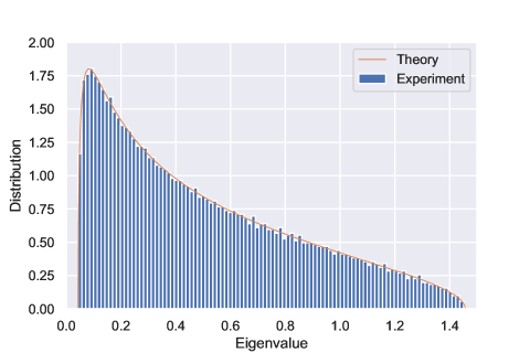
Figure S3: The eigenvalue distribution of the covariance matrix $\Lambda$. Here we set $\alpha=2$, $\sigma=0.5$ and $N=5000$.

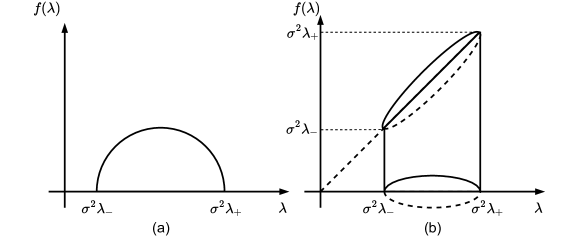
Figure S4: The calculation of spectrum moments by a geometric method. $f(\lambda)$ denotes the integrand of $I_{1}$ (a) or $I_{2}$ (b).

In the large $N$ limit, the normalized dimensionality of the matrix $\Lambda$ can be written in the form as follows,

$$\tilde{D}=\frac{\left(\sum_{i}\lambda_{i}\right)^{2}}{N\sum_{i}\lambda_{i}^{2}}=\frac{\left(\frac{1}{N}\sum_{i}\lambda_{i}\right)^{2}}{\frac{1}{N}\sum_{i}\lambda_{i}^{2}}=\frac{\left(\int d\lambda\rho(\lambda)\lambda\right)^{2}}{\int d\lambda\rho(\lambda)\lambda^{2}}\ .$$ (S74)

The numerator part is given by the first order moment of the eigen-spectrum,

$$I_{1} \stackrel{{\scriptstyle{\rm def}}}{{=}}\int d\lambda\rho(\lambda)\lambda$$ (S75)

$$=\frac{1}{2\pi\sigma^{2}}\int^{\lambda_{+}}_{\lambda_{-}}\sqrt{(\lambda-\sigma^{2}\lambda_{-})(\sigma^{2}\lambda_{+}-\lambda)}d\lambda$$

$$=\frac{1}{2\pi\sigma^{2}}\frac{1}{2}\pi\left[\frac{\sigma^{2}(\lambda_{+}-\lambda_{-})}{2}\right]^{2}$$

$$=\alpha\sigma^{2},$$

where we calculate the integral by computing the area of the semicircle shown in Fig. S4 (a). The denominator part is given by the second moment of the spectrum, computed as

$$I_{2} \stackrel{{\scriptstyle{\rm def}}}{{=}}\int d\lambda\rho(\lambda)\lambda^{2}$$ (S76)

$$=\frac{1}{2\pi\sigma^{2}}\int^{\lambda_{+}}_{\lambda_{-}}\lambda\sqrt{(\lambda-\sigma^{2}\lambda_{-})(\sigma^{2}\lambda_{+}-\lambda)}d\lambda$$

$$=\frac{1}{2\pi\sigma^{2}}\frac{1}{2}\pi\left[\frac{\sigma^{2}(\lambda_{+}-\lambda_{-})}{2}\right]^{2}\frac{\sigma^{2}(\lambda_{+}+\lambda_{-})}{2}$$

$$=\sigma^{4}\alpha(\alpha+1),$$

where the integral here can be transformed to half of the volume of the cylinder shown in Fig. S4 (b) [36]. Finally, we conclude that

$$\tilde{D}=\frac{I_{1}^{2}}{I_{2}}=\frac{\alpha}{\alpha+1},$$ (S77)

from which the normalized input dimensionality is independent of the input-pattern ($\bm{\xi}$) variance $\sigma^{2}$. This analytic result is confirmed in numerical simulations in the main text.

Appendix D Proof of $\upgamma_{1}\leq\upgamma_{2}$

In this section, we prove the relation $\upgamma_{1}\leq\upgamma_{2}$ at an arbitrary layer $l$, where $\upgamma_{1}=\overline{K_{ij}^{2}}/{\overline{K_{ii}}^{2}}$ and $\upgamma_{2}=\overline{K_{ii}^{2}}/\overline{K_{ii}}^{2}$. Because the denominators of $\upgamma_{1}$ and $\upgamma_{2}$ are the same, we just need to prove that $\overline{K_{ij}^{2}}\leq\overline{K_{ii}^{2}}$ where

$$\overline{K_{ii}^{2}} =\left<\left(\phi^{\prime}\left(\sqrt{g^{2}\mathcal{K}_{1}^{l-1}}t+x\sqrt{g^{2}Q^{l-1}+\sigma_{b}}\right)\right)^{4}\right>_{x,t}\ ,$$ (S78)

$$\overline{K_{ij}^{2}} =\left<\left<\phi^{\prime}\left(\sqrt{g^{2}\mathcal{K}_{1}^{l-1}}x+\sqrt{g^{2}Q^{l-1}}z_{1}+\sqrt{\sigma_{b}}u_{1}\right)\right>^{2}_{x}\right.$$

$$\left.\times\left<\phi^{\prime}\left(\sqrt{g^{2}\mathcal{K}_{1}^{l-1}}y+\sqrt{g^{2}Q^{l-1}}\left(\rho z_{1}+\sqrt{1-\rho^{2}}z_{2}\right)+\sqrt{\sigma_{b}}u_{2}\right)\right>^{2}_{y}\right>_{z_{1},z_{2},u_{1},u_{2}}\ .$$

Note that we add higher-order contributions of $\Delta_{ii}^{l}$ back into $\overline{K_{ii}^{2}}$, as mentioned in Sec. A.2. To proceed, we define $\vartheta_{x}\stackrel{{\scriptstyle{\rm def}}}{{=}}\sqrt{g^{2}\mathcal{K}_{1}^{l-1}}x+\sqrt{g^{2}Q^{l-1}}z_{1}+\sqrt{\sigma_{b}}u_{1}$ and $\vartheta_{y}\stackrel{{\scriptstyle{\rm def}}}{{=}}\sqrt{g^{2}\mathcal{K}_{1}^{l-1}}y+\sqrt{g^{2}Q^{l-1}}\left(\rho z_{1}+\sqrt{1-\rho^{2}}z_{2}\right)+\sqrt{\sigma_{b}}u_{2}$. Let $\langle\phi^{\prime}(\vartheta_{x})\rangle_{x}^{2}=\Phi_{1}$ and $\langle\phi^{\prime}(\vartheta_{y})\rangle_{y}^{2}=\Phi_{2}$. According to the Cauchy-Schwartz inequality, we have

$$\overline{\Phi_{1}\Phi_{2}}^{2}\leq\overline{\Phi_{1}^{2}}\cdot\overline{\Phi_{2}^{2}},$$ (S79)

where $\overline{\ \cdot\ }$ denotes the quenched disorder average as before. It is then easy to show that $\overline{\Phi_{2}^{2}}=\overline{\Phi_{1}^{2}}=\overline{K_{ii}^{2}}$. We finally conclude that $\upgamma_{1}\leq\upgamma_{2}$.

Appendix E Deep neural networks trained with Hebbian learning rules

To verify the revealed principles in this paper, we perform an on-line training of a layered neural network using the same transfer function, by applying the well-known Hebbian rule. We use the synthetic dataset generated in Sec. C, containing $10\ 000$ input samples ($\alpha=2$). These data samples are then sequentially shown to the input layer of the deep neural network, and then learned layer by layer. We use the synaptic rescaling to control the synaptic strength, like $w_{ij}(t)\leftarrow\frac{gw_{ij}(t)}{\sqrt{\sum_{k}w_{ik}^{2}(t)}}$, where $w_{ij}(t)$ is updated by the following regularized Hebbian rule:

$$w_{ij}^{l}(t)=w_{ij}^{l}(t-1)+\eta\left[h_{i}^{l}h_{j}^{l-1}-\kappa_{c}\left(\sum_{i^{\prime}:i^{\prime}\neq i}w_{i^{\prime}j}^{l}\right)\left(\sum_{k\neq k^{\prime}}^{N}w_{kj}^{l}w_{k^{\prime}j}^{l}-\sqrt{N}r\right)\right],$$ (S80)

where $t$ denotes the learning step, $N$ denotes the receptive field size of the hidden neuron at the $l$-th layer, $\eta$ is the learning rate, and $\kappa_{c}$ enforces the synaptic-correlation constraint, inspired by our theory. The last term in Eq. (S80) can be derived as the gradient descent of the correlation-constraint objective:

$$\Phi_{c}(\mathbf{w})=\frac{\kappa_{c}}{2}\sum_{j}\left[\sum_{i\neq i^{\prime}}^{N}w_{ij}w_{i^{\prime}j}-\sqrt{N}r\right]^{2},$$ (S81)

where the synaptic-correlation scaling derived in our paper is used for learning the continuous weights. The synaptic rescaling operation together with the synaptic-correlation constraint encourages synapses to compete with each other to encode input features during learning [27, 28].

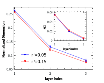
Figure S5: Dimension reduction and decorrelation in deep Hebbian learning with $N=100$. $\eta=0.0001$, $\kappa_{c}=0.5$, $g=0.5$, and $10\ 000$ training examples ($\alpha=2$) are sequentially (on line) shown to the input layer of deep networks. The result is averaged over ten random realizations.

As shown in Fig. S5, the regularized Hebbian learning rule is able to reduce the dimensionality of hidden representations, while decorrelating the representations as well. The qualitative behavior of the on-line trained systems coincides with the theoretical predictions of our model about roles of synaptic correlations. Therefore, it is promising to design unsupervised/supervised learning algorithms that can control the synaptic correlations in future works, e.g., in sensory perception of real-world datasets.

References

[1]
M. R. Cohen and A. Kohn.
Measuring and interpreting neuronal correlations.
Nat Neurosci, 14:811, 2011.
[2]
Felix Franke, Michele Fiscella, Maksim Sevelev, Botond Roska, Andreas
Hierlemann, and R. Silveira.
Structures of neural correlation and how they favor coding.
Neuron, 89(2):409–422, 2016.
[3]
Kanaka Rajan, L Abbott, and Haim Sompolinsky.
Inferring Stimulus Selectivity from the Spatial Structure of Neural
Network Dynamics.
In J. D. Lafferty, C. K. I. Williams, J. Shawe-Taylor, R. S. Zemel,
and A. Culotta, editors, Advances in Neural Information Processing
Systems 23, pages 1975–1983. Curran Associates, Inc., 2010.
[4]
N Brunel.
Is cortical connectivity optimized for storing information?
Nat Neurosci, 19:749–755, 2016.
[5]
Matthew Farrell, Stefano Recanatesi, Guillaume Lajoie, and Eric Shea-Brown.
Dynamic compression and expansion in a classifying recurrent network.
bioRxiv, 2019.
[6]
N. Alex Cayco-Gajic and R. Angus Silver.
Re-evaluating circuit mechanisms underlying pattern separation.
Neuron, 101(4):584–602, 2019.
[7]
Haiping Huang.
Mechanisms of dimensionality reduction and decorrelation in deep
neural networks.
Phys. Rev. E, 98:062313, 2018.
[8]
G. E. Hinton and R. R. Salakhutdinov.
Reducing the dimensionality of data with neural networks.
Science, 313(5786):504–507, 2006.
[9]
K. Harris and T Mrsic-Flogel.
Cortical connectivity and sensory coding.
Nature, 503:51–58, 2013.
[10]
K. Harris and G. Shepherd.
The neocortical circuit: themes and variations.
Nat Neurosci, 18:170–181, 2015.
[11]
Alexei A. Koulakov, Tomáš Hromádka, and Anthony M. Zador.
Correlated connectivity and the distribution of firing rates in the
neocortex.
The Journal of Neuroscience, 29(12):3685–3694, 2009.
[12]
Tianqi Hou, K. Y. Michael Wong, and Haiping Huang.
Minimal model of permutation symmetry in unsupervised learning.
Journal of Physics A: Mathematical and Theoretical, 52:414001,
2019.
[13]
Tianqi Hou and Haiping Huang.
Statistical physics of unsupervised learning with prior knowledge in
neural networks.
arXiv:1911.02344, 2019.
[14]
Alessandro Achille and Stefano Soatto.
Emergence of invariance and disentanglement in deep representations.
Journal of Machine Learning Research, 19(50):1–34, 2018.
[15]
Pagan Marino, Urban Luke S, Wohl Margot P, and Rust Nicole C.
Signals in inferotemporal and perirhinal cortex suggest an
untangling of visual target information.
Nat Neurosci, 16(8):1132–1139, 2013.
[16]
James J. DiCarlo and David D. Cox.
Untangling invariant object recognition.
Trends in Cognitive Sciences, 11(8):333–341, 2007.
[17]
See supplemental material at http://… for technical details of the theory and
simulation methods.
[18]
M. Mézard, G. Parisi, and M. A. Virasoro.
Spin Glass Theory and Beyond.
World Scientific, Singapore, 1987.
[19]
Chou P. Hung, Gabriel Kreiman, Tomaso Poggio, and James J. DiCarlo.
Fast Readout of Object Identity from Macaque Inferior Temporal
Cortex.
Science, 310(5749):863–866, 2005.
[20]
Thomas Serre, Aude Oliva, and Tomaso Poggio.
A feedforward architecture accounts for rapid categorization.
Proceedings of the National Academy of Sciences,
104(15):6424–6429, 2007.
[21]
Hong Ha, Yamins Daniel L K, Majaj Najib J, and DiCarlo James J.
Explicit information for category-orthogonal object properties
increases along the ventral stream.
Nat Neurosci, 19(4):613–622, 2016.
[22]
Alessio Ansuini, Alessandro Laio, Jakob H. Macke, and Davide Zoccolan.
Intrinsic dimension of data representations in deep neural networks.
arXiv:1905.12784, 2019.
in NeurIPS 2019.
[23]
Stefano Recanatesi, Matthew Farrell, Madhu Advani, Timothy Moore, Guillaume
Lajoie, and Eric Shea-Brown.
Dimensionality compression and expansion in deep neural networks.
arXiv:1906.00443, 2019.
[24]
Pau Rodriguez, Jordi Gonzalez, Guillem Cucurull, Josep M. Gonfaus, and
Xavier Roca.
Regularizing CNNs with locally constrained decorrelations.
arXiv:1611.01967, 2016.
in ICLR 2017.
[25]
Michael Cogswell, Faruk Ahmed, Ross Girshick, Larry Zitnick, and Dhruv
Batra.
Reducing overfitting in deep networks by decorrelating
representations.
arXiv:1511.06068, 2015.
in ICLR 2015.
[26]
Horace Barlow.
Possible principles underlying the transformation of sensory
messages.
In W. Rosenblith, editor, Sensory Communication, pages
217–234. Cambridge, Massachusetts: MIT Press, 1961.
[27]
Kenneth D. Miller and David J. C. MacKay.
The role of constraints in hebbian learning.
Neural Computation, 6(1):100–126, 1994.
[28]
H. Sebastian Seung and Jonathan Zung.
A correlation game for unsupervised learning yields computational
interpretations of hebbian excitation, anti-hebbian inhibition, and synapse
elimination.
arXiv:1704.00646, 2017.
[29]
D. Marr.
A Theory for Cerebral Neocortex.
Proceedings of the Royal Society of London B: Biological
Sciences, 176(1043):161–234, 1970.
[30]
Jeremie Barral and Alexander Reyes.
Synaptic scaling rule preserves excitatory-inhibitory balance and
salient neuronal network dynamics.
Nature Neuroscience, 19(12):1690–1696, 2016.
[31]
Andrew Saxe, Stephanie Nelli, and Christopher Summerfield.
If deep learning is the answer, then what is the question?
arXiv e-prints, page arXiv:2004.07580, 2020.
[32]
Demis Hassabis, Dharshan Kumaran, Christopher Summerfield, and Matthew
Botvinick.
Neuroscience-inspired artificial intelligence.
Neuron, 95(2):245–258, 2017.
[33]
Jakob H. Macke, Philipp Berens, Alexander S. Ecker, Andreas S. Tolias, and
Matthias Bethge.
Generating spike trains with specified correlation coefficients.
Neural Computation, 21(2):397–423, 2009.
[34]
S F Edwards and R C Jones.
The eigenvalue spectrum of a large symmetric random matrix.
Journal of Physics A: Mathematical and General,
9(10):1595–1603, oct 1976.
[35]
H. J. Sommers, A. Crisanti, H. Sompolinsky, and Y. Stein.
Spectrum of large random asymmetric matrices.
Phys. Rev. Lett., 60:1895–1898, 1988.