Achieving Fairness via Post-Processing in Web-Scale Recommender Systems

Abstract.

Building fair recommender systems is a challenging and crucial area of study due to its immense impact on society. We extended the definitions of two commonly accepted notions of fairness to recommender systems, namely equality of opportunity and equalized odds. These fairness measures ensure that equally “qualified” (or “unqualified”) candidates are treated equally regardless of their protected attribute status (such as gender or race). We propose scalable methods for achieving equality of opportunity and equalized odds in rankings in the presence of position bias, which commonly plagues data generated from recommender systems. Our algorithms are model agnostic in the sense that they depend only on the final scores provided by a model, making them easily applicable to virtually all web-scale recommender systems. We conduct extensive simulations as well as real-world experiments to show the efficacy of our approach.

1. Introduction

Fairness in classification (Agarwal et al., 2018b; Bechavod and Ligett, 2017) and ranking problems (Geyik et al., 2019) has been an active area of research in recent years due to its tremendous influence on society as a whole (Barocas et al., 2017). As more and more businesses rely on machine learning (ML) algorithms to recommend goods and services, treating affected individuals fairly is becoming ever more important. ML-based systems may contain implicit biases and can serve to reproduce or reinforce the biases present in society (Buolamwini and Gebru, 2018; Zou and Schiebinger, 2018). It is crucial to be able to mitigate these biases, especially in large-scale industrial applications.

Fairness mitigation strategies commonly fall into one of three categories: pre-, in-, or post-processing. Pre-processing modifies training data to reduce potential sources of bias, often by removing features that are correlated with protected attributes ((Zemel et al., 2013a; Calmon et al., 2017; Gordaliza et al., 2019)). In-processing (also known as training-time) mitigation methods modify the model training objective to incorporate fairness, often by adding constraints or regularization penalties (Kamishima et al., 2012; Bechavod and Ligett, 2017; Mary et al., 2019; Zafar et al., 2017b; Agarwal et al., 2018b). Finally, post-processing methods transform model scores to ensure fairness according to a provided definition. Post-processing methods learn (protected-attribute-specific) transformations of model scores to achieve fairness objectives (Hardt et al., 2016; Pleiss et al., 2017; Kamiran et al., 2012). They are very appealing in industrial practice as they do not require changes to an existing model training pipeline. Virtually any model can be easily adjusted by a post-processing algorithm to achieve the desired fairness goal.

In this paper, we derive post-processing approaches providing fairness for ranked lists of items generated by a recommender system. Hardt et al. (Hardt et al., 2016) introduce post-processing methods for equality of opportunity and equalized odds in the binary classification setting. However, these methods are not directly applicable to the ranking problems where fairness needs to hold with respect to the ranks of the items. Ranking problems are further complicated by the presence of position bias (Joachims et al., 2017; Wang et al., 2018), i.e., the bias in an end user’s response depending on an item’s position, which is not a concern in the binary classification setting. Geyik et al. (Geyik et al., 2019) provides an algorithm for fair ranking (informed by an approximation of equality of opportunity) by modifying the classification definition. This work does not address position bias, and the methodology does not extended to other notions of fairness, such as equalized odds.

Recently, there has been extensive work focused on framing fairness in ranking as an optimization problem maximizing relevance subject to fairness constraints (Celis et al., 2017; Singh and Joachims, 2018, 2019). These procedures are also limited in the types of fairness they can accommodate (largely addressing variations of equal exposure) and cannot be directly applied to fairness definitions incorporating outcomes such as equality of opportunity or equalized odds (Hardt et al., 2016). They are also impractical for many internet applications, where latency concerns may pose problems for solving an optimization problem for real-time queries.

We formally extend the definitions of equality of opportunity and equalized odds from the binary classification (Hardt et al., 2016) to the ranking context, provide a causal interpretation of the equalized odds condition (Section 3.3), and provide scalable post-processing techniques for mitigation of bias identified through these definitions, which has not been addressed by previous literature on fairness in ranking. We also explicitly handle the position bias issue and suggest simple mechanisms for controlling the fairness versus performance trade-off. Our novel method of enforcing equalized odds in ranking is highly flexible, and we show how it can be easily extended to tackle multiple outcomes and appropriate relaxations. We perform extensive experiments to showcase the efficacy of our procedure by considering simulated, public, and real-world datasets.

The remainder of the paper is organized as follows. We first define and then develop post-processing techniques to adjust for equality of opportunity and equalized odds in rankings (Section 2 and Section 3 respectively). We address the position bias issues present in the ranking context for both the mechanisms in Section 4. We empirically show the efficacy of our approach in Section 5 before concluding with a discussion in Section 6. Proofs of all results are given in the Appendix in the supplementary material. We end this section with a brief overview of the related literature.

1.1. Related Work

Most early work in fairness has been on classification tasks and strives to achieve fairness notions such as equalized odds on protected attributes (Agarwal et al., 2018b; Hardt et al., 2016; Feldman et al., 2015; Zafar et al., 2017a; Zafar et al., 2017c; Goh et al., 2016; Wu et al., 2019). Also, many techniques for training models that guarantee other definitions of fairness, such as equality opportunity (Hardt et al., 2016) and demographic parity, have been widely studied in recent years (Dwork et al., 2012a; Zemel et al., 2013b; Goel et al., 2018; Johndrow et al., 2019). Penalty methods for incorporating fairness constraints during model training has received a great deal of attention (Kamishima et al., 2012; Bechavod and Ligett, 2017; Mary et al., 2019; Zafar et al., 2017b). Although they are sound theoretical methods, many of them do not scale well due to the iterative nature of these algorithms (Agarwal et al., 2018b) and hence can become a bottleneck in many large-scale applications. Thus, post-processing techniques, which are model-agnostic, are often preferable.

Many large-scale recommender systems are ranking systems, returning a list of ranked results to the users. Although there are several scalable post-processing methodologies (Hardt et al., 2016; Pleiss et al., 2017; Kamiran et al., 2012) for fairness, most of them focus on classification problems, and they do not directly translate to the ranking problem. Moreover, position bias plays a critical role in these ranking frameworks, which we address through our post-processing reranker. Several works handle fairness in recommender systems by solving a constrained optimization to optimize for relevance, subject to fairness constraints (Singh and Joachims, 2018; Celis et al., 2017). These techniques are broadly applicable but suffer from two drawbacks. First, they are limited in the types of fairness they can address and are limited to addressing variations of equal exposure (and cannot be applied to fairness definitions incorporating outcomes such as equality of opportunity). Second, they are impractical for many internet applications, where latency concerns may pose problems for solving an optimization problem for real-time queries. (Geyik et al., 2019) provides an algorithm for fair recommendations informed by an approximation of equality of opportunity through an approximation to the classification definition. However, this work lacks a meaningful extension of this fairness notion to the ranking setting and does not address equalized odds. There have also been works addressing fairness in Learning-to-Rank applications (Singh and Joachims, 2019; Morik et al., 2021) which is beyond the scope of this paper.

2. Equality of Opportunity in Rankings

Throughout, we assume that a machine learning model predicts an outcome $Y$ from available features $X$ resulting in a score $s(X)$ (or simply $s$ for compactness). These predictions are used to provide ranked recommendations of people or items where each recommendation is assumed to have a categorical group characteristic $C$ (e.g., protected attribute status). Before discussing equality of opportunity for ranking, we will recall the definition of equality of opportunity (EOpp) for binary classification (Hardt et al., 2016). In the binary classification context, machine learning models yield a binary prediction $\hat{Y}$ which can but need not be derived from a score $s(X)$.

Definition 2.1 (EOpp in classification).

A binary predictor $\hat{Y}$ satisfies equal opportunity with respect to a (protected) characteristic $C$ if $\hat{Y}$ is independent of $C$ given $Y=1$, that is,

$$\mathbb{P}(\hat{Y}=1\mid C=c_{1},Y=1)=\mathbb{P}(\hat{Y}=1\mid C=c_{2},Y=1),~{}\text{for all $c_{1},c_{2}$.}$$

In other words, $\hat{Y}$ is independent of $C$ given that $Y=1$.

A useful extension of this condition beyond binary model outputs is to the case when the model outputs scores. In this setting, we require that the distribution of model scores be be independent of $C$ given that $Y=1$ (see, e.g., (Mary et al., 2019), Section 2.1). For threshold based classifiers (i.e., ones for which  $\hat{Y}(X)=1$ if and only if $s(X)>t$ for an appropriate threshold $t$), this would ensure EOpp for the associated classifiers at all thresholds.

Definition 2.2 (EOpp in rankings).

A scoring function satisfies equal opportunity with respect to a (protected) characteristic $C$ and score $s(X)$ if for all $c_{1}$, $c_{2}$ and $t$,

$$\mathbb{P}(s(X)\leq t\mid C=c_{1},Y=1)=\mathbb{P}(s(X)\leq t\mid C=c_{2},Y=1),~{}\text{}.$$

In industry applications, Definition 2.2 is a natural requirement as scores could be passed downstream to other machine learning systems before yielding final recommendations. Even in the case of classification, applying the “ranking” definition of EOpp can be preferable. One reason is that in many internet applications, the threshold $t$ for a score based classifier is chosen through A/B experimentation to yield a desirable tradeoff of business metrics (Agarwal et al., 2018a). As such, it is generally not known a priori which threshold is needed, and this definition affords the robustness and flexibility of guaranteeing fairness regardless of the threshold chosen. Note that the solution proposed in (Hardt et al., 2016) is based on Definition 2.1, while in the following subsection, we propose a solution based on Definition 2.2.

2.1. Algorithm to achieve Equality of Opportunity:

In the following lemma, we present a simple post-processing algorithm that achieves EOpp at all thresholds $t$ simultaneously. Define the cumulative distribution function (CDF) of scores in group $C=c$ and $Y=1$ by

$$F_{c,1}(t)=\mathbb{P}(s(X)\leq t\mid C=c_{1},Y=1)=\mathbb{P}(s(X)\leq t\mid C=c,Y=1)~{}.$$

Applying an appropriate CDF transformation to the model scores achieves EOpp .

Lemma 2.3 (Algorithm for EOpp ).

Let $F_{c,1}(\cdot)$ be the cumulative distribution function (CDF) of scores in group $C=c$ and $Y=1$. Then for each $c$, the transformation of the scores of group $C=c$ as $s(X)\to F_{c,1}(s(X))$, will guarantee EOpp for all thresholds $t$.

The CDF transformations in Lemma 2.3 maps the scores into $[0,1]$. We can apply an additional transformation $F^{-1}(\tilde{F}(\cdot))$ to bring the scores back to the original scale, where $F$ and $\tilde{F}$ are the CDF of the scores before applying any transformation and after applying the transformations in Lemma 2.3, respectively. Note that this step will not affect the EOpp problem, since $F^{-1}(\tilde{F}(\cdot))$ is a monotonic transformation. This step might be useful in industrial settings where scores are used in more than one machine learning systems. This line of reasoning is similar to quantile normalization in (bio)statistics (Amaratunga and Cabrera, 2001; Bolstad et al., 2003).

2.2. Variants of EOpp algorithm:

These post-processing approaches also allow us to maintain EOpp between retraining of the models by updating the $F_{c,1}$’s online, as user engagement can be changing dynamically, requiring adjustment to the algorithm (D’Amour et al., 2020). In practice, we discretize (for instance, at every percentile or every $10^{-4}$) the CDFs corresponding to the EOpp transformation and create a linear or higher-order interpolation between the points for applying the transformation. Next, note that the algorithm immediately generalizes to an arbitrary number of characteristics. Furthermore, one could relax the strict EOpp constraint, by considering the following modification to the transformation of the scores:

(1) $$\widetilde{s}_{c}(\alpha)=\alpha\times F^{-1}(\tilde{F}(F_{c,1}(s_{c})))+(1-\alpha)\times s_{c},$$

where $s_{c}$ denote the score restricted to $C=c$ and $\alpha\in[0,1]$ is a tuning parameter for linearly mixing the original score with the transformed score. We can tune $\alpha$ to achieve a desirable performance-fairness trade-off (if needed), where larger values of $\alpha$ would bring more fairness (in terms of EOpp), possibly at the expense of lower model performance.

3. Equalized Odds in Rankings

Equalized odds (EOdds) is a fairness definition which extends equality of opportunity. In the context of binary classification, (Hardt et al., 2016) defines equalized odds as follows.

Definition 3.1 (EOdds in classification).

A binary predictor satisfies equalized odds with respect to a (protected) characteristic $C$ and decision $\hat{Y}$, if $\hat{Y}$ is independent of $C$ given $Y$, that is, $\mathbb{P}(\hat{Y}=1\mid C=c_{1},Y=y)=\mathbb{P}(\hat{Y}=1\mid C=c_{2},Y=y)$ for all $c_{1},c_{2}\text{ and }y\in\{0,1\}$.

Similarly to the EOpp definition, the EOdds definition can be naturally extended to handle the ranking case, where ranks are assigned according to a scoring function $s(X)$.

Definition 3.2 (EOdds in rankings).

A scoring function satisfies equalized odds with respect to a (protected) characteristic $C$ and score $s(X)$ if $\mathbb{P}(s(X)\leq t\mid C=c_{1},Y=y)=\mathbb{P}(s(X)\leq t\mid C=c_{2},Y=y)$ for all $c_{1},c_{2},t\text{ and }y\in\{0,1\}$. That is, the score distribution is independent of $C$ given the outcome $Y$.

This is equivalent to the requirement that the distribution of the scores is independent of $C$ given the outcome $Y$. Unlike EOpp , EOdds cannot be achieved through a deterministic transformation. (Hardt et al., 2016) provide a randomization mechanism to change binary classification labels in such a way that the derived prediction satisfies EOpp . We will now review the binary classification setting, and develop a methodology for the ranking context.

3.1. Re-Ranking for Equalized Odds:

In the context of classifiers, EOdds can be achieved by randomizing classifications as follows. Consider randomly changing the decision of a classification $\hat{Y}=y$ for group $C=c$ with probability $p_{y,c}$. The resulting randomized classification, satisfies equalized odds whenever the following set of linear constraints are satisfied for all $c_{1}$, $c_{2}$ and $y$:

$$(1-p_{y,c_{1}})\cdot\mathbb{P}(\hat{Y}=y\mid C=c_{1},Y=y)~{}+$$

$$\qquad\qquad p_{1-y,c_{1}}\cdot\mathbb{P}(\hat{Y}=1-y\mid C=c_{1},Y=y)$$

$$= (1-p_{y,c_{2}})\cdot\mathbb{P}(\hat{Y}=y\mid C=c_{2},Y=y)~{}+$$

$$\qquad\qquad p_{1-y,c_{2}}\cdot\mathbb{P}(\hat{Y}=1-y\mid C=c_{2},Y=y).$$

We extend this reasoning to the ranking context. Without loss of generality, assume that the ranking scores $s(\cdot)$ fall in the interval $[0,1)$. Note that if the scores do not fall in this interval, they can easily be transformed to this interval in a way that does not affect rankings, for instance, by applying an inverse logit transformation.

Let $I_{1},...,I_{K}$ be a partition of the score domain. That is, choose intervals $I_{k}=[i_{k},i_{k+1})$ for $k=1,...,K$, where $0=i_{1}<i_{2}<\cdots<i_{K+1}=1$. We will derive a score achieving equalized odds by randomizing the original scores between these intervals. For each category $C=c_{i}$, define $p_{k,k^{\prime},c_{i}}$ (such that $\sum_{k^{\prime}}p_{k,k^{\prime},c_{i}}=1$ for all $k$ and $c_{i}$) to be the probability that the score from an item with characteristic $c_{i}$ is randomly moved from interval indexed by $k$ to interval indexed by $k^{\prime}$ (for notational compactness, we will write $P$ as the set of these probabilities). Let $Z_{k,c_{i}}$ be a multinomial random variable with probabilities $(p_{k,1,c_{i}},\ldots,p_{k,K,c_{i}})$. Then, for an item with characteristic $C=c_{i}$ and score $s(X)\in I_{k}$, we define $\bar{s}(X;P)$ (or more compactly $\bar{s}(X)$) to be a score chosen in the interval $I_{Z_{k,c_{i}}}$ according to an arbitrary (for instance, uniform) distribution on $I_{Z_{k,c_{i}}}$. Note that,

$$~{}\mathbb{P}(\bar{s}(X)\in I_{k^{\prime}}\mid C=c_{i},Y=y)$$

(2) $$= ~{}\sum\nolimits_{k}p_{k,k^{\prime},c_{i}}\cdot\mathbb{P}(s(X)\in I_{k}\mid C=c_{i},Y=y).$$

Consequently, the randomized score $\bar{s}(X)$ satisfies equalized odds whenever $p_{k,k^{\prime},c_{i}}$’s are chosen to satisfy $\mathbb{P}(\bar{s}(X)\in I_{k^{\prime}}\mid C=c_{1},Y=y)=\mathbb{P}(\bar{s}(X)\in I_{k^{\prime}}\mid C=c_{2},Y=y)$ for all $k^{\prime}$ and $y\in\left\{0,1\right\}$. It is readily seen from Equation (3.1) that this specifies a system of linear equations in the interval transition probabilities $P=\{p_{k,k^{\prime},c_{i}}\}$. Not only does a solution to this system always exist, but there are infinitely many solutions. Ideally, we would like to use a solution which gives good model performance. To identify a “best” solution, let $\phi(F_{X,Y,C},P)$ be a functional of the data generating distribution $F_{X,Y,C}(\cdot)$ and the interval transition probabilities $P$ such that $\phi(F_{X,Y,C},P)$ captures some aspect of predictive performance such as mean squared error or area under the receiver operating characteristic curve (ROC-AUC). Note that $F_{X,Y,C}(\cdot)$ is generally not known, but is easily replaced by the empirical version in such situations. Finding the optimal interval transition probabilities can be formulated as a maximization problem

$$\max_{P}~{}~{}\phi\left(F_{X,Y,C},P\right)~{}\text{such that}~{}$$

$$\quad\sum\nolimits_{k}p_{k,k^{\prime},c_{i}}\cdot\mathbb{P}(s(X)\in I_{k}\mid C=c_{1},Y=y)$$

(3) $$= \quad\sum\nolimits_{k}p_{k,k^{\prime},c_{i}}\cdot\mathbb{P}(s(X)\in I_{k}\mid C=c_{2},Y=y)$$

for all $c_{1}$, $c_{2},k^{\prime}$, and $y\in\{0,1\}$.

Theorem 3.3.

The randomized score $\bar{s}(X)$ derived from $s(X)$ using interval transition probabilities found as the solution to the optimization problem (3.1) satisfies

$$\mathbb{P} (\bar{s}(X)\leq t\mid C=c_{1},Y=y)=\mathbb{P}(\bar{s}(X)\leq t\mid C=c_{2},Y=y),$$

for all $c_{1}$, $c_{2}$, $y$, and $t$.

While the choice of the objective function $\phi$ can be arbitrary, we give two suggestions. One choice is to define $\phi$ as ${\mathbb{E}}\left(|s(X)-\bar{s}(X)|\right)$, which gives the least possible average movement of the scores, which were originally chosen to give good performance. The empirical version of this condition can easily be written as a linear equation, which gives the computational convenience that the optimization problem (3.1) becomes a linear program (LP). Another choice is to maximize for ROC-AUC which boils down to solving a quadratic program (QP) (See Appendix for details).

Let $P^{*}=\{p_{k,k^{\prime},c_{i}}^{*}\}$ denote the solution of (3.1). Then, to apply the EOdds transformation to each score $s(X)\in I_{k}$ corresponding to an item in $c_{i}$, we just need to sample from a multinomial distribution with probabilities $(p_{k,1,c_{i}}^{*},\ldots,p_{k,K,c_{i}}^{*})$ to choose a destination bin index and sample from a, for instance, uniform distribution on the chosen bin. This shows the scalability of the proposed solution.

Time complexity: In practice, the EOpp/EOdds transformation works by observing the initial score, finding its score bucket, and allocating it to a different score bucket based on a pre-computed mapping for EOpp and based on a pre-computed probability vector for EOdds. Finding the score bucket corresponding to the initial score can be done in $log(K)$ (or even constant) time, where $K$ is the number of score buckets. Allocating it to a different score bucket can be done in O(1) time using HashMaps for EOdds (trivially for EOpp). As the number of items $n$ increases, the new final list can be obtained in $O(nlog(K))$ time.

Choice of bins: Note that the choice of bins are arbitrary but obvious choices include equispaced bins or quantile binning. We recommend choosing intervals based on quantiles for EOpp. However, we experimented with equispaced bins for the EOdds transformation in our social network application and still got a good performance. For EOdds, we note that finer binnings typically result in less degredation to model performance, however in our empirical evaluations (including a social network application), we saw little benefit from using more than 100 equispaced bins or from using quantiles instead of equispaced bins. Given modern linear program solvers can easily handle thousands of bins, we encourage practitioners to use as fine a binning as practical subject to suitable model performance.

3.2. Extensions of Equalized Odds:

EOdds has several natural extensions such as to general categorical outcomes that are easily handled by adjustments to the constraints in the optimization based methodology for re-ranking. Suppose that items are ranked according to a score $s(X)$, and the rankings result in an outcome $y\in{1,...,M}$. For example, in a news feed context, users of a site may engage with articles in multiple ways captured by actions such as “like,” “comment,” or “share.” We extend the definition of equalized odds to ensure that the rankings are fair with respect to any of these outcomes across all characteristics.

Definition 3.4 (Multi-Outcome EOdds in Rankings).

A score based ranker satisfies equalized odds with respect to (protected) characteristic $C$ and score $s(X)$ if

$$\mathbb{P}(s(X)\leq t \mid C=c_{1},Y=y)=\mathbb{P}(s(X)\leq t\mid C=c_{2},Y=y),$$

for all $c_{1}$, $c_{2}$, $y\in\left\{1,...,M\right\}$ and $t$.

Achieving multi-outcome EOdds simply requires extending the linear constraints in optimization problem (3.1) to all $y\in\left\{1,..,M\right\}$. When finding a randomized scoring function as a solution to this modified optimization problem, an analogous result to Theorem 3.3 holds, but for multi-outcome EOdds.

Another simple modification is to relax the strictness of the equalized odds condition.

Definition 3.5 ($\epsilon_{0},\epsilon_{1}$-differentially EOdds in Rankings).

A score based ranker satisfies $\epsilon_{0},\epsilon_{1}$-differentially equalized odds with respect to (protected) characteristic $C$ and score $s(X)$ if

$$\exp{(-\epsilon_{y})}\leq\frac{\mathbb{P}(s(X)\leq t\mid C=c_{1},Y=y)}{\mathbb{P}(s(X)\leq t\mid C=c_{2},Y=y)}\leq\exp{(\epsilon_{y})}$$

for all $c_{1}$, $c_{2}$, $t$ and $y\in\{0,1\}$.

Ensuring that a randomized ranking score $\bar{s}(X)$ satisfies $\epsilon_{0},\epsilon_{1}$-differentially EOdds requires conditions that can be expressed as linear constraints, for example through

$$\mathbb{P}(\bar{s}(X)\leq t \mid C=c_{1},Y=1)-\exp{(\epsilon)}\mathbb{P}(\bar{s}(X)\leq t\mid C=c_{2},Y=1)\leq 0$$

and similarly for the remaining constraints required. Once again, a simple modification of the constraints in optimization problem (3.1) leads to a randomized ranking score such that an analogous result to Theorem 3.3 holds, but for $\epsilon_{0},\epsilon_{1}$-differentially EOdds . An interesting special case is $\infty,\epsilon_{1}$-differentially equalized odds, which reduces to $\epsilon_{1}$-differentially EOpp, providing a method to re-rank for an alternative relaxation of EOpp. Adjusting the $\epsilon_{0},\epsilon_{1}$ allows the practitioner to strike a desireable balance between fairness and model performance.

3.3. Causal Interpretation of Equalized Odds:

We conclude this section by providing an interpretation of EOdds using causal graphs. A causal graph is a directed acyclic graph (DAG) where the nodes represent variables, and the directed edges in the graph define conditional independence relationships among the variables via the notion of d-separation (Pearl, 2000). The conditional independence between the scoring variable $s(X)$ (or $S$ in short) and the characteristic $C$ given the observed outcome $Y$ (Definition 3.2) can be represented by the absence of paths from $C$ to $S$ that are not d-separated by $Y$ in the underlying causal DAG. We illustrate this through the following examples.

For simplicity, we assume that no variable has a causal influence on $C$ and $S$ has no causal influence on any variable. These assumptions are reasonable in most situations where $C$ is an exogenous variable representing gender, race, or age, and $S$ is generated through machine learning models based on $Y$ and other variables. The causal DAG corresponding to our first example is depicted in Figure 1a. In this case, the EOdds is not satisfied due to the existence of the directed path $C\to X_{2}\to S$ that does not go through $Y$. In other words, the EOdds condition prohibits the characteristic $C$ from having a causal influence on the score $S$ except through the observed outcome $Y$. In the DAG given in Figure 1b, the path $C\to X_{1}\leftarrow X_{2}\to S$ from $C$ to $S$ is not d-separated by $Y$ since $Y$ is a child of the collider node $X_{1}$. In other words, the EOdds condition prohibits a conditional dependency between the characteristic $C$ and the score $S$ given $Y$ through ”selection bias” (Pearl, 2009; Elwert and Winship, 2014). Finally, the DAG in Figure 1c satisfies EOdds since $Y$ is a non-collider node on the only path $C\to Y\to S$ from $C$ to $S$, and hence $C$ and $S$ are d-separated by $Y$.

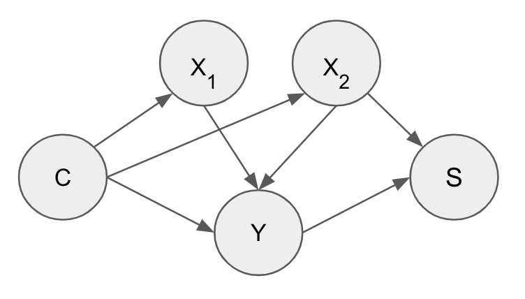
1a EOdds is not satisfied due to the existence of the directed path $C\to X_{2}\to S$.

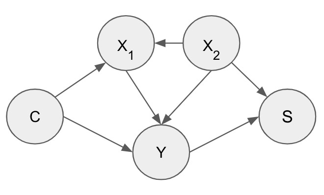
1b EOdds is not satisfied due to the existence of the collider path $C\to X_{1}\leftarrow X_{2}\to S$ and the directed edge $X_{1}\to Y$.

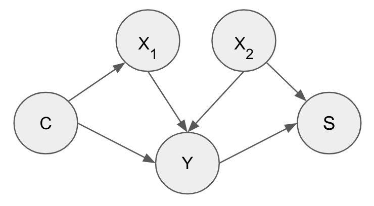
1c EOdds is satisfied since the only directed path from $C$ to $S$ is d-separated by $Y$.

4. Position Bias Adjustment

To understand the effect of position bias in achieving EOpp and EOdds, consider a recommendation system where for each query $q$, a candidate set of $J$ items $\{d^{(q)}_{1},\ldots,d^{(q)}_{J}\}$ are ranked according to a scoring function $s(X)$ defined on a set of features $X$. The viewer’s response to $d^{(q)}_{i}$ in the recommended list not only depends on the quality of $d^{(q)}_{i}$ (relative to the viewer) but also depends on the position of $d^{(q)}_{i}$ in the list. The position bias refers to the fact that the chance of observing a positive response (e.g.,  a click) on an item appearing at a higher position (where the highest position is Position 1) is higher than the chance of observing the same in a lower position. We emphasize that both observed and unobserved items are considered for defining position bias. Consequently, our definition of position bias covers all biases that are due to the position at which an item is ranked, including selection bias (Oosterhuis and de Rijke, 2020; Ovaisi et al., 2020) and trust bias (Agarwal et al., 2019; Vardasbi et al., 2020). Selection bias (users only observing the items ranked in the top k positions), and trust bias (having a higher likelihood to click a higher ranked item among the observed items) both stem from the position at which an item is ranked.

To define EOpp or EOdds in the presence of the position bias, we need to take into account the dependency of the response variable $Y$ on the position where the item is shown. To this end, we denote the counterfactual response of an item appearing at position $j$ by $Y(j)$. Furthermore, we denote by $\gamma$ the position of an item in the ranking generated by $s(X)$. Therefore, the observed response is given by $Y(\gamma)$.

Definition 4.1.

A scoring function $s(X)$ of a recommendation system satisfies EOpp or EOdds with respect to a characteristic $C$ if

(4) $$\mathbb{P}(s(X)\leq t\mid C=c_{1},Y(\gamma)=y)=\mathbb{P}(s(X)\leq t\mid C=c_{2},Y(\gamma)=y),$$

for all $t,c_{1},c_{2}$, and for $y=1$ for EOpp and $y\in\{0,1\}$ for EOdds.

Note that the post-processing approaches discussed in the previous section work under the assumption that $Y(j)$’s are identical for all $j$. To see this, let $\tilde{s}(X)$ denote the score of an item after applying the EOpp or EOdds post-processing algorithm and let $\tilde{\gamma}$ denote the corresponding position of the item in the ranking generated by $\tilde{s}(X)$. Then $(\tilde{s}(X),\gamma)$ would satisfy (4) for $\gamma$ equals the position of the item in the ranking without post-processing. However, this does not guarantee that $(\tilde{s}(X),\tilde{\gamma})$ would satisfy (4) unless $Y(j)$’s are identical for all $j$. Below, we propose adjustments to the EOpp and EOdds algorithms for satisfying (4) under the following assumptions on the position bias:

Assumption 1.

For all queries $q$ and all candidate items $d^{(q)}_{i}$ and all $j>1$, we assume

1. Homogeneity: $\mathbb{P}\big{(}Y(j)=1\mid Y(1)=1,~{}d^{(q)}_{i}\big{)}=\mathbb{P}(Y(j)=1\mid Y(1)=1)$, and

2. Preservation of Hierarchy: $\mathbb{P}\big{(}Y(j)=1\mid Y(1)=0,~{}d^{(q)}_{i}\big{)}=0.$

The first assumption states that the position bias is homogeneous over all queries and candidate items. This is a common assumption in the literature (Singh and Joachims, 2018, 2019; Wang et al., 2018). The second assumption states that if a candidate item in a given position does not get a positive response, it cannot get a positive response in a lower position (which is reasonable in most practical settings). Under Assumption 1, we formally define the position bias as the following positive response decay factor:

(5) $$w_{j}:=\mathbb{P}(Y(j)=1\mid Y(1)=1)~{}\text{for $j=1\ldots,J$.}$$

4.1. Tackling Position Bias for Equality of Opportunity:

We achieve Eq. (4) for EOpp by learning the conditional CDFs of weighted scores (c.f. Lemma 2.3) where the weights are given by the inverse of the decay factor defined in Eq. (5).

Theorem 4.2.

Let $w_{j}$ be as in Equation (5) and let $F_{c,1}^{*}(\cdot)$ denote the CDF of the conditional scores $s(X)$ given $Y(\gamma)=1$ and $C=c$ with weights $1/w_{\gamma}$. Under Assumption 1, the transformed scores $\tilde{s}(X):=\sum_{c}F_{c,1}^{*}(s(X))1_{\{C=c\}}$ satisfy

1. $\mathbb{P}(\tilde{\gamma}=j\mid C=c_{1},~{}Y(1)=1)=\mathbb{P}(\tilde{\gamma}=j\mid C=c_{2},~{}Y(1)=1)$, and

2. $\mathbb{P}(\tilde{s}(X)\leq t\mid C=c_{1},~{}Y(\tilde{\gamma})=1)=\mathbb{P}(\tilde{s}(X)\leq t\mid C=c_{2},~{}Y(\tilde{\gamma})=1),$

for all $j$, $t$ and $c_{1},c_{2}$, where $\tilde{\gamma}$ denotes the position of an item based on $\tilde{s}(X)$.

The first part of Theorem 4.2 shows that the weighted CDF transformations guarantee “fairness of exposure” with respect to the items with a (counterfactual) positive response at position 1. This is also related to the notion of group fairness parity in (Singh and Joachims, 2019).

Corollary 4.3.

For a characteristic $C=c$, let $M_{c}:=\mathbb{P}(Y(1)=1\mid C=c)$ and $v_{obs}(c):=\mathbb{P}(Y(\tilde{\gamma})=1\mid C=c)$ be the average merit and the observed exposure (with respect to the scoring function $\tilde{s}(X)$ defined in Theorem 4.2), respectively. Then under Assumption 1, $\tilde{s}(X)$ achieves the group fairness parity, given by the following constraint: $v_{obs}(c_{1})/M_{c_{1}}=v_{obs}(c_{2})/M_{c_{2}},~{}\text{for all}~{}c_{1},c_{2}.$

4.2. Tackling Position Bias for Equalized Odds:

We achieve Equation (4) for EOdds by carefully adjusting the counts of positive and negative labels in certain data segments defined by $\{C=c,Y(\gamma)=y,s(X)\in I_{k},\gamma=j\}$. To motivate our approach, we first show that if we had access to the counterfactual label $Y(1)$, then the method defined in the previous section would have worked. Then we describe how we can estimate $\mathbb{P}(\tilde{s}(X)\in I_{k}\mid C=c,Y(1)=y)$ by adjusting for the position bias.

Theorem 4.4.

Under Assumption 1, let $\tilde{s}(X)$ be such that $\mathbb{P}(\tilde{s}(X)\leq t\mid C=c_{1},Y(1)=y)=\mathbb{P}(\tilde{s}(X)\leq t\mid C=c_{2},Y(1)=y),$ for $k\in\{1,\ldots,K\}$, $y\in\{0,1\}$ and for all $c_{1},c_{2}$. Then $\tilde{s}(X)$ satisfies the equalized odds conditions given in Definition 4.1.

To use Theorem 4.4 in conjunction with the optimization given in (3.1), we need to estimate the counterfactual probabilities $\mathbb{P}(s(X)\in I_{k}\mid C=c,Y(1)=y)$ for all $c$, $y$ and $k$. To this end, we define the adjusted positive and negative label counts at position $j$ as follows.

$$n_{c,1,k}^{(j)\prime}=n_{c,1,k}^{(j)}/w_{j}~{}\text{and}~{}n_{c,0,k}^{(j)\prime}=(n_{c,0,k}^{(j)}+n_{c,1,k}^{(j)})-n_{c,1,k}^{(j)\prime},$$

where $n_{c,y,k}^{(j)}:=\sum_{r}1_{\{C_{r}=c,~{}Y_{r}(\gamma_{r})=y,~{}s(X_{r})\in I_{k},~{}\gamma_{r}=j\}}$ is the observed count and $w_{j}$ is the positive response decay factor defined in (5). Then we estimate $\mathbb{P}(s(X)\in I_{k}\mid C=c,Y(1)=y)$ as

(6) $$\hat{\mathbb{P}}(s(X)\in I_{k}\mid C=c,Y(1)=y)=\frac{\left(\sum\nolimits_{j}n_{c,y,k}^{(j)\prime}\right)}{\left(\sum\nolimits_{j,k}n_{c,y,k}^{(j)\prime}\right)}.$$

We prove the correctness of this adjustment in Theorem 4.5.

Theorem 4.5.

Under Assumption 1, $\hat{\mathbb{P}}(s(X)\in I_{k}\mid C=c,Y(1)=y)$ converges to $\mathbb{P}(s(X)\in I_{k}\mid C=c,Y(1)=y)$ almost surely for all $k,c,y$.

4.3. Position Bias Estimation:

The weighted CDF transformations defined in Theorem 4.2 and the estimation of the counterfactual probabilities $\mathbb{P}(s(X)\in I_{k}\mid C=c,Y(1)=y)$ via (6) require the positive response decay factors $w_{j}$’s defined in (5) to be known or estimated. To estimate $w_{j}$, we may collect data by randomizing slots and estimate $w_{j}$ as the ratio of the number of positive responses at position $j$ and position $1$, i.e.

(7) $$\hat{w}_{j}=\frac{(\sum_{r}1_{\{Y_{r}(\gamma)=1,~{}\gamma_{r}=j\}})/(\sum_{r}1_{\{\gamma_{r}=j\}})}{(\sum_{r}1_{\{Y_{r}(\gamma)=1,~{}\gamma_{r}=1\}})/(\sum_{r}1_{\{\gamma_{r}=1\}})}.$$

Without randomization, we will end up underestimating $w_{j}$ by using Equation (7) as the items served at position $j$ are expected to be of lower quality than the items served at position 1. More precisely, in the observational data where the items are ranked according to $s(X)$, the conditional distribution of $s(X)$ given $\gamma=1$ is expected to be stochastically larger than that of $s(X)$ given $\gamma=j$. However, randomly shuffling all items can undesirably harm viewers’ experience. A less harmful alternative is to shuffle pairs of items randomly (Joachims et al., 2017; Wang et al., 2018). To estimate the weights from observational data, (Wang et al., 2018) applied the EM algorithm with a parametric click model. Below, we propose a non-parametric approach to estimate the weights from observational data based on importance sampling. To this end, we first estimate the response bias at position $j$ relative to position $j-1$ by correcting for the discrepancy in the distribution of scores in those positions with importance weighting as follows.

Let $f_{j}(\cdot)$ denote the conditional density of the observed score at position $j$. For $j\geq 2$, define

(8) $$\eta_{j}=\frac{{\mathbb{E}}\left(Y(\gamma)\frac{f_{j-1}(s(X))}{f_{j}(s(X))}\mid\gamma=j\right)}{{\mathbb{E}}\left(Y(\gamma)\mid\gamma=j-1\right)}.$$

It is straightforward to estimate $\eta_{j}$ by replacing the conditional density and the conditional expectations with the corresponding empirical estimates. We denote this estimator by $\hat{\eta}_{j}$. Finally, we estimate $w_{j}$ by $\hat{w}_{j}=\prod_{r=2}^{j}\hat{\eta}_{r}$. We establish the correctness of this method in the following theorem.

Theorem 4.6.

Under Assumption 1, $\eta_{j}$ defined in (8) equals $\mathbb{P}(Y(j)=1\mid Y(1)=1)~{}/~{}\mathbb{P}(Y(j-1)=1\mid Y(1)=1)$ and hence, $w_{j}$ defined in (5) equals $\prod_{r=2}^{j}\eta_{r}$.

The reason for not estimating the $w_{j}$ directly by using the importance weights $f_{1}(s(X))/f_{j}(s(X))$ is that the distribution of scores at position $1$ might be much different from its counterpart at position $j$, even for not-so-large large $j$. Our adjacent-pairwise importance sampling approach tends to have a lower variance than the direct importance sampling approach since the score distributions of the adjacent positions are expected to be relatively close to each other. However, for practical purposes we recommend to use a truncated version $\hat{w}_{j}=\prod_{r=2}^{\min(j,T)}\hat{\eta}_{r}$ for some threshold $T$. This is equivalent to assuming $\eta_{j}=1$ for all $j>T$, which is a reasonable practical assumption for most recommendation systems. The overall algorithms for position adjusted EOpp and EOdds are given below.

4.4. Position Bias Adjusted Algorithms

Algorithm 1 Position Bias Adjusted Equality of Opportunity

1:Reranker Training

2:Input: Score, position, label and characteristic data $(s_{i},\gamma_{i},y_{i},c_{i})$, $i=1,...,n$

3:Compute the weighted empirical CDF $\hat{F}_{c,1}^{*}$ of the conditional scores $s(X)$ given $Y(\gamma)=1$ and $C=c$ with weights $1/\hat{w}_{\gamma}$ computed as in Section “Position Bias Adjustment”

4:Output: The empirical distribution functions $\hat{F}_{c,1}^{*}$

5:Reranker Scoring

6:Input: Score $S$, characteristic $C$

7:Output: Fair score, $\tilde{S}=\sum_{c}\hat{F}_{c,1}^{*}(S)1_{\{C=c\}}$

Algorithm 2 Position Bias Adjusted Equalized Odds

1:Reranker Training

2:Input: Score, position, label and characteristic data $(s_{i},\gamma_{i},y_{i},c_{i})$, $i=1,...,n$ and a partition of the score space $I_{1},...,I_{K}$

3:Estimate empirical conditional bin probabilities as in (6) with weights estimated as in Section “Position Bias Adjustment”

4:Find $P$, the solution to Optimization Problem (3.1)

5:Output: Vector of interval transition probabilities, $P$

6:Reranker Scoring

7:Input: Score $S$, characteristic $C$, a partition of the score space $I_{1},...,I_{K}$, interval transition probabilities $P=\{p_{k,k^{\prime},c}\}$ and distribution functions $F_{1},\ldots,F_{K}$

8:Determine $k$ such that $S\in I_{k}$

9:Choose $k^{\prime}$ from a multinomial distribution with probabilities $\{p_{k,1,C},\ldots,p_{k,K,C}\}$

10:Randomly select a point $\tilde{S}$ within $I_{k}$ according to $F_{k}(\cdot)$

11:Output: Fair score, $\tilde{S}$

5. Empirical Evaluation

We do a thorough simulation study to validate the need and the efficacy of our algorithms to achieve fairness in web-scale recommender systems. Note that this validation cannot be done with a publicly available dataset since the labels in a validation data must be generated after reranking items with our post-processing algorithms in order to capture the effect of the position bias. Next, we demonstrate the scalability of our methods with an application on a connection recommendation system in a real-life social network platform.

The simulation and empirical studies shown here are to demonstrate that the proposed methods exactly satisfy the stated definitions of fairness (namely EOpp and EOdds ), with limited impact on (and potentially even improvement to) model performance. Existing work in fairness for recommendation systems considers fairness definitions other than EOpp and EOdds and we cannot make meaningful comparisons between fairness definitions, nor can we interpret differences in model performance changes (e.g. stricter notions of fairness often yield larger impact on model predictive performance). For this reason, we omit comparisons with methods of achieving differing notions of fairness and leave the choice of the appropriate fairness criteria to the domain expertise of practitioners who can best assess the suitability of various fairness criteria to the problem at hand. Please see the discussion section below for more on the choice of fairness metrics.

5.1. Simulation Study:

We generate a population of $p=50000$ items, where each item consists of id $i$, characteristic $C_{i}\sim\{0,1\}$, $Y_{i}(1)\in\{0,1\}$ and relevance $R_{i}$. We independently generate $C_{i}$’s from a $\textit{Bernoulli }(0.6)$ distribution. The conditional distribution $Y_{i}(1)$ given $C_{i}=0$ is $\textit{Bernoulli }(0.4)$, and the conditional distribution $Y_{i}(1)$ given $C_{i}=1$ is $\textit{Bernoulli }(0.5)$. Finally, $R_{i}\mid(C_{i},Y_{i}(1))$ is generated from

$$\mathcal{N}(0.6Y_{i}(1)+2C_{i},~{}0.5)+(1-C_{i})\textit{Uniform }[0,~{}(1+Y_{i}(1))].$$

We consider a recommendation system with $K=50$ slots. For each query, we randomly select $50$ items from the population and assign a score $s_{i}=R_{i}+\mathcal{N}(0,0.1)$ to each selected item $i\in\{1,\ldots,50000\}$. The selected items are then ranked according to $s_{i}$ (in a descending order) and assigned position according to $\textrm{rank}(i)$. Finally, the item at position $j$ gets observed response $Y(j)=Y(1)\times\textit{Bernoulli }(w_{j})$ with position bias $w_{j}=1/\log_{2}(1+j)$. We generate a training dataset based on $100000$ queries and a validation dataset based on $50000$ queries.

Results: We use the adjacent-pairwise importance sampling approach with the threshold $T=30$ for the position bias estimation based on the training dataset. Next, we learn the weighted empirical CDF for EOpp based on the training data. To learn the position bias-adjusted EOdds re-ranker based on the training data, we apply an inverse-logit transformation to the score, discretize the score using 100 equally spaced intervals and solve the optimization problem given in (3.1) with ${\mathbb{E}}\left(|s(X)-\bar{s}(X)|\right)$ as the objective function.

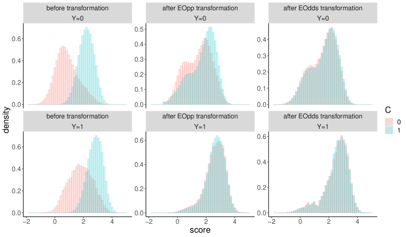
Figure 2. Score distributions before and after EOpp and EOdds transformations.

We apply these transformations on the validation data scores and each time regenerate the online labels (with position bias) based on the rankings of the items given by the transformed scores. Figure 2 validates the usefulness of our algorithms in achieving EOpp and EOdds . Prior to these transformations, it is seen that the conditional score distributions differ greatly between the characteristics. Post-transforming, the conditional score distributions are identical, as required for equalized odds. Recall that the EOpp transformation only guarantees to produce identical score distributions across all groups for positive labels, while EOdds guarantees the same for positive labels as well as for negative labels. These are reflected in Figure 2.

We implemented the Algorithms in R. Based on the training data with 5 million samples (100k queries with 50 slots), the position bias estimation took 7 seconds, the EOpp learning took 9 seconds, and the EOdds learning with 100 bins took 100 seconds on a Macbook Pro with 3.5 GHz Dual-Core Intel Core i7 processor and 16 GB 2133 MHz LPDDR3 memory, demonstrating the scalability of the proposed algorithms.

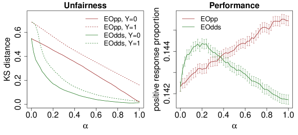
Figure 3. Unfairness and performance for different $\alpha$.

Finally, Figure 3 demonstrates how a desirable performance-fairness trade-off can be achieved via a linear combination of the transformed scores and the original scores given by,

$$\alpha\times(\textrm{transformed~{}score})+(1-\alpha)\times(\textrm{original score}),$$

where $\alpha\in[0,1]$ is a tuning parameter (see (1)). Unfairness and performance are measured via Kolmogorov-Smirnov distance (measuring the closeness of the conditional score distributions between groups) and proportion of positive responses respectively. Note that EOpp and EOdds are both specified through equating conditional distributions and hence a distribution distance metric (such as the Kolmogorov-Smirnov distance) is a natural choice for measuring “unfairness” (or deviations from the desired fairness condition). The performance measured through the proportion of positive labels (cf. click-through-rate in online recommendations) and the error bars in the figure represent one standard deviation of uncertainty. Here, we observe the following:

1. The unfairness decreases to zero as $\alpha$ increases, except for EOpp corresponding to negative labels (as expected).

2. The unfairness corresponding to the EOpp transformation is strictly lower for all values of $\alpha$, while the performance of EOpp is strictly better for $\alpha\geq 0.4$.

3. The performance corresponding to the EOpp transformation is monotonically increasing with $\alpha$. This serves as a counterexample to the popular belief that fairness and performance are always conflicting properties of recommender systems. The improvement in performance by enforcing fairness has also been observed in some recent works (Bello and Honorio, 2020; Islam et al., 2021; Maity et al., 2020). We note that this is possible, for example, when a more relevant group of candidates gets underexposed through a recommendation system (and we can achieve a correct exposure through unfairness mitigation).

5.2. Social Network Application:

Friend or connection recommendation systems are used by many large social network companies such as Facebook, Instagram, LinkedIn, etc. These systems suggests members to connect with others, in order to build their network. Here, a member sending an invitation to connect with a suggested candidate can be viewed as a positive outcome. We apply our methodology to (proprietary) training data used for such a product containing historical recommendations and labels indicating whether an invitation has been sent. Members are categorized as infrequent members (IMs; members who are less active on the platform) or frequent members (FMs) who tend to have greater rates of engagement and correspondingly higher representation in the training data. In this example there is potential for the model to not only be biased against IMs, but for that bias to be reinforced over time, leading to a system that is optimized for the benefit of members who are already highly engaged on the site (also known as “popularity bias” or the “rich getting richer” phenomenon (Abdollahpouri et al., 2019)).

We see an opportunity to apply fairness notions, as a debiasing mechanism, to adjust for the exposure of IMs as candidates being recommended, thus giving them opportunities to be shown and invited. In our experiments, we applied both the EOpp and EOdds reranker to give qualified IMs and FMs equal representation in recommendations. We build the required transformations using two weeks of training data. While serving we apply the transformation on the top 100 candidates. The serving was done via a discretized CDF (with 10000 points) for EOpp and through the estimated transition probabilities (based on 100 bins) for EOdds. Due to the simple transformation in both approaches, we did not see any drastic gain in latency, which is a core-requirement in large-scale recommender systems. The results of the A/B tests on real member traffic are shown in Table 1.

Invitation	Equality of Opportunity		Equalized Odds
Metrics	IM	FM	IM	FM
Sent	+ 5.72%	Neutral	+ 2.77%	Neutral
Accepted	+ 4.85%	Neutral	+ 2.26%	Neutral

Table 1. A/B Experimentation results for rerankers.

Two of the cornerstone metrics for evaluating such experiments are invitations sent and invitations accepted. While one might expect that this post-processing approach would shift invitations away from FMs to IMs and may be detrimental to the metrics for FMs, we were heartened to see more invites being sent to and accepted by IMs without any statistically significant negative impact (pvalue ¿ 0.05) on the FMs. This highlights that re-ranking approaches pursuing fairness have improved overall recommendation quality.

6. Discussion

We have proposed post-processing methods for handling equality of opportunity and equalized odds in relevance score-based rankings and suggested simple mechanisms for controlling the fairness versus performance trade-off. Our post-processing approaches are applicable in many internet-industry applications as they are tailored towards scalability, have a relatively low engineering footprint, and, unlike in-processing methods, can be relatively easily added on top of existing machine-learning/AI pipelines.

We explicitly handled the position bias issue while implicitly assuming that the labels are unbiased. In the presence of label bias, methodology such as (Jiang and Nachum, 2020), which provides a mechanism for imputing debiased labels, can be applied prior to the methods developed in this paper. We considered equality of opportunity and equalized odds as the definition of fairness, which amounts to providing equal opportunity or exposure to equally qualified candidates in a ranking irrespective of their protected attribute status. Here equal qualification is determined by the observed response (i.e., $Y=1$ corresponds to qualified candidates) after correcting for position bias. We note that there are several other existing definitions of fairness that we do not cover in this work, including predictive rate parity (Zafar et al., 2017a), demographic parity (Dwork et al., 2012b), counterfactual fairness (Kusner et al., 2017). These fairness criteria are often conflicting (Saravanakumar, 2021), and the choice of a fairness criterion should be application-specific.

The relative merits of various fairness definitions has been studied in other works including (Corbett-Davies et al., 2017) and (Corbett-Davies and Goel, 2018) and we encourage practitioners to familiarize themselves with the possible benefits and pitfalls before deciding on a fairness criteria. Equality of opportunity may be an appropriate choice when balancing exposure of recommendations resulting in a “positive” outcome is across groups is desirable and equalized odds may be useful when balancing exposure conditional on any outcome label is important. Works such as (Jacobs et al., 2013) and (Aygün and Bó, 2021) demonstrate how well-intentioned fairness initiatives can lead to unintended consequences. Ultimately, we leave it to the practitioners to use their domain expertise to judge the applicability of equality of opportunity or equalized odds and suggest that users carefully monitor the results of fairness mitigation over time to safeguard against any unforeseen harm.

This research can benefit groups that are currently disadvantaged by large-scale automatic decision systems. While we do not see any clear negative outcomes of this work, we remain mindful that fairness is a dynamic problem, and we have addressed it from a static perspective. This work has also not addressed intersectionality explicitly, though the framework can handle some intersectional questions. Good practice requires monitoring the fairness performance of the tools we have developed and as well as assessing whether they have unintended intersectional consequences.

7. Appendix

7.1. Equalized Odds in Rankings

In the main text, we described how we can solve for Equalized Odds when we define $\phi$ as ${\mathbb{E}}\left(|s(X)-\bar{s}(X)|\right)$. Here we give the details when we choose $\phi$ as the ROC-AUC.

A Riemann approximation to the ROC-AUC based on the partition $I_{1},...,I_{K}$ can be computed as

$$\sum\nolimits_{c} \mathbb{P}(C=c)\cdot\sum\nolimits_{k=1}^{K}\mathbb{P}(\bar{s}(X)\in I_{k}\mid Y=0)\sum\nolimits_{k^{\prime}\geq k}\mathbb{P}(\bar{s}(X)\in I_{k^{\prime}}\mid Y=1).$$

It is readily seen from Equation (3.1) that this is a quadratic function of the transition probabilities. Therefore, when using this choice of objective, the optimization problem (3.1) becomes a quadratic program (QP) with $K^{2}\cdot L\cdot(L-1)$ variables for a characteristic $C$ with $L$ categories.

7.2. Position Bias Estimation

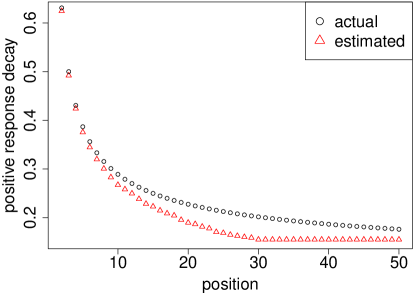
Figure 4. Estimating the position bias $w_{j}=1/\log 2(1+j)$ for $j=2,\ldots,50$, using the adjacent-pairwise importance sampling approach with the threshold $T=30$.

We use the estimator $\hat{w}_{j}=\prod_{r=2}^{\min(j,T)}\hat{\eta}_{r}$ with $T=30$ defined in Section “Position Bias Adjustment” to estimate the position bias for each $j=2,\ldots,50$. Although we estimate each $\eta_{r}$ unbiasedly, but the product of the estimators of $\eta_{r}$’s is no longer guaranteed to be unbiased. This explains the underestimation pattern in Figure 4. We deliberately chose a simulation setting where the estimation of $w_{i}$ is challenging to demonstrate the insensitivity of our mitigation techniques to the position bias estimation errors.

7.3. Proofs

• Let $s_{c,1}$ denote the random variable corresponding to the score $s(X)$ restricted to $C=c$ and $Y=1$. Since $F_{c,1}$ is the CDF of $s_{c,1}$, the distribution of $F_{c,1}(s_{c,1})$ is $Uniform[0,1]$ for all $c$. Hence these transformed scores satisfy equality of opportunity across all thresholds. ∎

• We first prove the results using the following claims and then prove the claims.
   
  Claim 1: For all $j>1$ and for all $t$,

  $$~{}P(s(X)\leq t\mid\gamma=j,~{}Y(j)=1,~{}C=c)$$

  $$= ~{}P(s(X)\leq t\mid\gamma=j,~{}Y(1)=1,~{}C=c).$$

  
  

  Claim 2: For all $j>1$,

  $$P(\gamma=j \mid Y(\gamma)=1,~{}C=c)=\frac{w_{j}P(\gamma=j\mid Y(1)=1,~{}C=c)}{\sum_{r}w_{r}P(\gamma=r\mid Y(1)=1,~{}C=c)}.$$

  Using Claims 1 and 2, we show that the CDF of $s(X)$ given $Y(1)=1$ and $C=c$ equals $F_{c,1}^{*}$.

  $$\quad F_{c,1}^{*}(t)$$

  $$:=~{}\sum_{j}\bigg{\{}P(s(X)\leq t\mid\gamma=j,~{}Y(j)=1,~{}C=c)~{}\frac{P(\gamma=j\mid Y(\gamma)=1,C=c)/w_{j}}{\sum_{r}P(\gamma=r\mid Y(\gamma)=1,C=c)/w_{r}}\bigg{\}}$$

  $$=~{}\sum_{j}\bigg{\{}P(s(X)\leq t\mid\gamma=j,~{}Y(1)=1,~{}C=c)~{}\frac{P(\gamma=j\mid Y(1)=1,C=c)}{\sum_{r}P(\gamma=r\mid Y(1)=1,C=c)}\bigg{\}}$$

  $$=~{}\sum_{j}\big{\{}P(s(X)\leq t\mid\gamma=j,~{}Y(1)=1,~{}C=c)~{}P(\gamma=j\mid Y(1)=1,C=c)\big{\}}$$

  $$=~{}\sum_{j}P(s(X)\leq t,~{}\gamma=j\mid Y(1)=1,~{}C=c)$$

  $$=~{}P(s(X)\leq t\mid Y(1)=1,~{}C=c).$$

  The first equality follows from the definition of $F_{c,1}^{*}$, we use Claims 1 and 2 in the second equality, the third equality follows from the fact that $\sum_{j}P(\gamma=j\mid Y(1)=1,C=c)=1$, and the fourth equality follows from the fact that

  $$\cup_{j}\big{(}\{s(X)\leq t\}\cap\{\gamma=j\}\big{)}=\{s(X)\leq t\}.$$

  We have shown that the conditional distribution of $s(X)$ given $Y(1)=1$ and $C=c$ equals $F_{c,1}^{*}$. This implies that the conditional distribution of $\tilde{s}(X):=F_{c,1}^{*}(s(X))$ given $Y(1)=1$ and $C=c$ is $Uniform[0,~{}1]$ for all $c$. Therefore, the conditional distributions of the position $\tilde{\gamma}$ given $Y(1)=1$ and $C=c$ are identical for all $c$. To see this, note that

  (9) $$P(\tilde{\gamma}\leq j \mid Y(1)=1,~{}C=c)=P(\tilde{s}(X)>U_{(K-j)}\mid Y(1)=1,~{}C=c),$$

  where $K$ is the total number of positions, $U_{(0)}=0$ and for $j<K$, $U_{(K-j)}$ is the $(K-j)$-th order statistic corresponding to $K$ i.i.d. uniform samples. Note that the right hand side of (9) does not depend on $c$ since the conditional distribution of $\tilde{s}(X):=F_{c,1}^{*}(s(X))$ given $Y(1)=1$ and $C=c$ is $Uniform[0,~{}1]$ for all $c$. This completes the proof of the first part of the theorem.

  To prove the second part, we will use Claims 1 and 2 with $(\tilde{s}(X),~{}\tilde{\gamma})$ instead of $(s(X),~{}\gamma)$.

  $$\quad P(\tilde{s}(X)\leq t\mid C=c,~{}Y(\tilde{\gamma})=1)$$

  $$=\sum_{j}\bigg{\{}P(\tilde{s}(X)\leq t\mid\tilde{\gamma}=j,~{}Y(j)=1,~{}C=c)~{}P(\tilde{\gamma}=j\mid Y(\tilde{\gamma})=1,C=c)\bigg{\}}$$

  $$=\frac{\sum_{j}w_{j}~{}P(\tilde{s}(X)\leq t,~{}\tilde{\gamma}=j\mid Y(1)=1,~{}C=c)}{\sum_{r}w_{r}P(\tilde{\gamma}=r\mid Y(1)=1,C=c)}.$$

  Now note that it follows from the first part of theorem that the denominator is identical for each $c$. Furthermore, the numerator does not depend on $c$, since it follows from (9) and the independence of $(\tilde{s}(X)\mid Y(1)=1)$ and $C$ that

  $$~{}P(\tilde{s}(X)\leq t,~{}\tilde{\gamma}=j\mid Y(1)=1,~{}C=c)$$

  $$= ~{}P(U_{(K-j)}<\tilde{s}(X)\leq\min\{U_{(K-j+1)},~{}t\}\mid Y(1)=1).$$

  This completes the second part of the theorem.
   
  Proof of Claim 1: From the second part of Assumption 1, it follows that

  $$~{}P(s(X)\leq t\mid\gamma=j,~{}Y(j)=1,~{}C=c)$$

  $$= ~{}P(s(X)\leq t\mid\gamma=j,~{}Y(j)=1,~{}Y(1)=1,~{}C=c).$$

  Therefore, the results follows from the first part of Assumption 1 that ensures that $Y(j)$ is independent of $s(X)$,  $\gamma$ and $C$ given $Y(1)$.
   
  Proof of Claim 2: For notational convenience, we denote the conditional probabilities given $C=c$ by $P_{c}(\cdot)$. Using the second part of Assumption 1 and then applying the Bayes’ theorem, we get

  $$~{}P_{c}(\gamma=j\mid Y(\gamma)=1)$$

  $$= ~{}P_{c}(\gamma=j\mid Y(\gamma)=1,~{}Y(1)=1)$$

  $$= ~{}\frac{P_{c}(Y(\gamma)=1\mid Y(1)=1,~{}\gamma=j)P_{c}(\gamma=j\mid Y(1)=1)}{\sum_{r}P_{c}(Y(\gamma)=1\mid Y(1)=1,~{}\gamma=r)P_{c}(\gamma=r\mid Y(1)=1)}$$

  $$= ~{}\frac{P(Y(j)=1\mid Y(1)=1)P_{c}(\gamma=j\mid Y(1)=1)}{\sum_{r}P(Y(r)=1\mid Y(1)=1)P_{c}(\gamma=r\mid Y(1)=1)}$$

  $$= ~{}\frac{w_{j}P_{c}(\gamma=j\mid Y(1)=1)}{\sum_{r}w_{r}P_{c}(\gamma=r\mid Y(1)=1)}.$$

  The seconds last equality follows from the first part of Assumption 1, and the last equality follows from the definition of $w_{j}$. ∎

• For notational convenience, we denote the conditional probabilities given $C=c$ by $P_{c}(\cdot)$. Note that

  $$\frac{v_{obs}(c)}{M_{c}} =\frac{\sum_{j}P_{c}(Y(j)=1\mid Y(1)=1,~{}\tilde{\gamma}=j)P_{c}(Y(1)=1,~{}\tilde{\gamma}=j)}{P_{c}(Y(1)=1)}$$

  $$=\frac{\sum_{j}P(Y(j)=1\mid Y(1)=1)P_{c}(Y(1)=1,~{}\tilde{\gamma}=j)}{P_{c}(Y(1)=1)}$$

  $$=\sum_{j}w_{j}P_{c}(\tilde{\gamma}=j\mid Y(1)=1),$$

  where $w_{j}$ is as in Theorem 4.2 and the second equality follows from the first part of Assumption 1. Therefore, the result follows from the first part of Theorem 4.2. ∎

• Fix a $t\in[0,1)$. Assume $t\in I_{k}$, i.e. $i_{k}\leq t<i_{k+1}$. Then,

  $$~{}P(\bar{s}(X)\leq t\mid C=c,Y=y)$$

  $$= ~{}P(\bar{s}(X)\leq t\mid\bar{s}(X)\in I_{k},C=c,Y=y)~{}\times~{}P(\bar{s}(X)\in I_{k}\mid C=c,Y=y)$$

  $$= ~{}F_{k}(t)~{}\times~{}P(\bar{s}(X)\in I_{k}\mid C=c,Y=y)$$

  Now, $F_{k}(t)$ does not depend on $y$ or $c$, and the constraints satisfied in the optimization problem imply that $P(\bar{s}(X)\in I_{k}\mid C=c,Y=y)$ does not depend on $c$ conditionally on $y$. It follows that equalized odds is satisfied in the ranking sense. ∎

• Note that without loss of generality, we can assume that the $\tilde{s}(X))$ given $Y(1)=1$ and $C=c$ is $Uniform[0,1]$. This is because we can transform the score using the same CDF function (since they have the same distribution) to make them $Uniform[0,1]$ for all $c$. Then it follows from the arguments given the proof of Theorem 4.2 that $P(\tilde{s}(X)\leq t\mid C=c,~{}Y(\tilde{\gamma})=1)$ is independent of $c$. ∎

• For notational convenience, we denote the conditional probabilities given $C=c$ by $P_{c}(\cdot)$. By applying Bayes’ Theorem, we get

  $$\mathbb{P}_{c}(s(X)\in I_{k} \mid Y(1)=y)~{}=~{}\frac{\mathbb{P}_{c}(Y(1)=y,~{}s(X)\in I_{k})}{\sum_{\ell}\mathbb{P}_{c}(Y(1)=y,~{}s(X)\in I_{\ell})}.$$

  Next, note that

  $$\qquad\mathbb{P}_{c}(Y(1)=1,~{}s(X)\in I_{\ell})$$

  $$=~{}\sum_{j}\mathbb{P}_{c}(Y(1)=1,~{}\gamma=j,~{}s(X)\in I_{\ell}).$$

  $$=~{}\sum_{j}\bigg{\{}\mathbb{P}_{c}(s(X)\in I_{\ell}\mid Y(1)=1,~{}\gamma=j)~{}\times~{}\mathbb{P}(Y(1)=1,~{}\gamma=j)\bigg{\}}$$

  $$=~{}\sum_{j}\bigg{\{}\mathbb{P}_{c}(s(X)\in I_{\ell}\mid Y(j)=1,~{}\gamma=j)~{}\times~{}\mathbb{P}_{c}(Y(1)=1,~{}\gamma=j)\bigg{\}}$$

  $$=~{}\sum_{j}\frac{\mathbb{P}_{c}(s(X)\in I_{\ell},Y(j)=1,~{}\gamma=j)}{\mathbb{P}_{c}(Y(j)=1\mid Y(1)=1,~{}\gamma=j)}$$

  $$=~{}\sum_{j}\frac{\mathbb{P}_{c}(s(X)\in I_{\ell},Y(j)=1,~{}\gamma=j)}{\mathbb{P}(Y(j)=1\mid Y(1)=1)}$$

  $$=~{}\sum_{j}\frac{\mathbb{P}_{c}(s(X)\in I_{\ell},Y(j)=1,~{}\gamma=j)}{w_{j}}.$$

  The first, second and the fourth equalities follow from the definition of conditional probability, the third equality follows from Claim 1 in the proof of Theorem 4.2, the fifth equality follows from Assumption 1 and the last equality follows from the definition of $w_{j}$.

  Now it follows from the strong law of large numbers that $\frac{n_{c,1,\ell}^{(j)}}{n_{c}}$ converges almost surely to $\mathbb{P}_{c}(s(X)\in I_{\ell},Y(j)=1,~{}\gamma=j)$, where $n_{c}$ is the number of samples corresponding to $C=c$. Hence, we have

  $$\hat{\mathbb{P}}_{c}(s(X)\in I_{k}\mid Y(1)=1)\overset{a.s}{\longrightarrow}\mathbb{P}_{c}(s(X)\in I_{k}\mid Y(1)=1),$$

  where $\overset{a.s}{\longrightarrow}$ denotes almost sure convergence.

  Finally, note that

  $$\mathbb{P}_{c}(Y(1)=0,~{}s(X)\in I_{\ell})$$

  $$=~{} \mathbb{P}_{c}(s(X)\in I_{\ell})-\mathbb{P}_{c}(Y(1)=1,~{}s(X)\in I_{\ell})$$

  $$=~{} \mathbb{P}_{c}(s(X)\in I_{\ell})-\sum_{j}\frac{\mathbb{P}_{c}(s(X)\in I_{\ell},Y(j)=1,~{}\gamma=j)}{w_{j}}.$$

  Therefore, $\hat{\mathbb{P}}_{c}(s(X)\in I_{k}\mid Y(1)=0)\overset{a.s}{\longrightarrow}\mathbb{P}_{c}(s(X)\in I_{k}\mid Y(1)=0)$ follows from the strong law of large numbers similarly. ∎

• Note that

  $${\mathbb{E}}\left(Y(\gamma)\frac{f_{j-1}(s(X))}{f_{j}(s(X))}\mid\gamma=j\right)$$

  $$=~{} \int{\mathbb{E}}\left(Y(\gamma)\frac{f_{j-1}(z)}{f_{j}(z))}\mid\gamma=j,s(X)=z\right)f_{j}(z)dz$$

  $$=~{} \int\mathbb{P}(Y(j)=1\mid\gamma=j,~{}s(X)=z)~{}f_{j-1}(z)dz$$

  $$=~{} \int\mathbb{P}(Y(j)=1\mid Y(1)=1,~{}\gamma=j-1,~{}s(X)=z)~{}\times$$

  $$\qquad\qquad~{}\mathbb{P}(Y(1)=1\mid\gamma=j,~{}s(X)=z)f_{j-1}(z)dz$$

  $$=~{} \mathbb{P}(Y(j)=1\mid Y(1)=1)~{}\times~{}\int\mathbb{P}(Y(1)=1\mid s(X)=z)~{}f_{j-1}(z)dz.$$

  The second last equality follows from the Preservation of Hierarchy assumption in Assumption 1, and the last equality follows from the Homogeneity assumption in Assumption 1. Similarly, we have

  $$~{}E\left[Y(\gamma)\mid\gamma=~{}j-1\right]$$

  $$= ~{}P(Y(j-1)=1\mid Y(1)=1)\times\int P(Y(1)=1\mid s(X)=z)f_{j-1}(z)dz.$$

  This completes the proof of the first part of the theorem, and the second part follows directly from the first part as $P(Y(j-1)=1\mid Y(1)=1)=1$ for $j=2$. ∎

References

- (1)
- Abdollahpouri et al. (2019) Himan Abdollahpouri, Masoud Mansoury, Robin Burke, and Bamshad Mobasher. 2019. The unfairness of popularity bias in recommendation. arXiv preprint arXiv:1907.13286 (2019).
- Agarwal et al. (2018b) Alekh Agarwal, Alina Beygelzimer, Miroslav Dudik, John Langford, and Hanna Wallach. 2018b. A Reductions Approach to Fair Classification. In Proceedings of the 35th International Conference on Machine Learning, Vol. 80. PMLR, 60–69.
- Agarwal et al. (2019) Aman Agarwal, Xuanhui Wang, Cheng Li, Michael Bendersky, and Marc Najork. 2019. Addressing Trust Bias for Unbiased Learning-to-Rank. In The World Wide Web Conference (WWW ’19). Association for Computing Machinery, New York, NY, USA, 4–14.
- Agarwal et al. (2018a) Deepak Agarwal, Kinjal Basu, Souvik Ghosh, Ying Xuan, Yang Yang, and Liang Zhang. 2018a. Online Parameter Selection for Web-based Ranking Problems. In KDD (London, United Kingdom). ACM, New York, NY, USA, 23–32.
- Amaratunga and Cabrera (2001) Dhammika Amaratunga and Javier Cabrera. 2001. Analysis of Data From Viral DNA Microchips. J. Amer. Statist. Assoc. 96, 456 (2001), 1161–1170. https://doi.org/10.1198/016214501753381814
- Aygün and Bó (2021) Orhan Aygün and Inácio Bó. 2021. College Admission with Multidimensional Privileges: The Brazilian Affirmative Action Case. American Economic Journal: Microeconomics 13, 3 (2021), 1–28.
- Barocas et al. (2017) Solon Barocas, Moritz Hardt, and Arvind Narayanan. 2017. Fairness in machine learning. NIPS Tutorial 1 (2017).
- Bechavod and Ligett (2017) Yahav Bechavod and Katrina Ligett. 2017. Penalizing Unfairness in Binary Classification. (2017). arXiv:1707.00044.
- Bello and Honorio (2020) Kevin Bello and Jean Honorio. 2020. Fairness constraints can help exact inference in structured prediction. In Advances in Neural Information Processing Systems 33: Annual Conference on Neural Information Processing Systems 2020, NeurIPS 2020.
- Bolstad et al. (2003) B.M. Bolstad, R.A Irizarry, M. Åstrand, and T.P. Speed. 2003. A comparison of normalization methods for high density oligonucleotide array data based on variance and bias. Bioinformatics 19, 2 (01 2003), 185–193. https://doi.org/10.1093/bioinformatics/19.2.185
- Buolamwini and Gebru (2018) Joy Buolamwini and Timnit Gebru. 2018. Gender shades: Intersectional accuracy disparities in commercial gender classification. In Conference on fairness, accountability and transparency. PMLR, 77–91.
- Calmon et al. (2017) Flavio Calmon, Dennis Wei, Bhanukiran Vinzamuri, Karthikeyan Natesan Ramamurthy, and Kush R Varshney. 2017. Optimized Pre-Processing for Discrimination Prevention. In Advances in Neural Information Processing Systems, I. Guyon, U. V. Luxburg, S. Bengio, H. Wallach, R. Fergus, S. Vishwanathan, and R. Garnett (Eds.), Vol. 30. Curran Associates, Inc., 3992–4001.
- Celis et al. (2017) L. Elisa Celis, Damian Straszak, and Nisheeth K. Vishnoi. 2017. Ranking with Fairness Constraints. arXiv:1704.06840 [cs.DS]
- Corbett-Davies and Goel (2018) Sam Corbett-Davies and Sharad Goel. 2018. The Measure and Mismeasure of Fairness: A Critical Review of Fair Machine Learning. arXiv:1808.00023 [cs.CY]
- Corbett-Davies et al. (2017) Sam Corbett-Davies, Emma Pierson, Avi Feller, Sharad Goel, and Aziz Huq. 2017. Algorithmic Decision Making and the Cost of Fairness (KDD ’17). Association for Computing Machinery, New York, NY, USA, 797–806. https://doi.org/10.1145/3097983.3098095
- Dwork et al. (2012a) Cynthia Dwork, Moritz Hardt, Toniann Pitassi, Omer Reingold, and Richard Zemel. 2012a. Fairness through awareness. In Proceedings of the 3rd innovations in theoretical computer science conference. 214–226.
- Dwork et al. (2012b) Cynthia Dwork, Moritz Hardt, Toniann Pitassi, Omer Reingold, and Richard Zemel. 2012b. Fairness through Awareness. In Proceedings of the 3rd Innovations in Theoretical Computer Science Conference (ITCS ’12). Association for Computing Machinery, New York, NY, USA, 214–226.
- D’Amour et al. (2020) Alexander D’Amour, Hansa Srinivasan, James Atwood, Pallavi Baljekar, D. Sculley, and Yoni Halpern. 2020. Fairness is Not Static: Deeper Understanding of Long Term Fairness via Simulation Studies. In Proceedings of the 2020 Conference on Fairness, Accountability, and Transparency (FAT* ’20). Association for Computing Machinery, 525–534.
- Elwert and Winship (2014) Felix Elwert and Christopher Winship. 2014. Endogenous Selection Bias: The Problem of Conditioning on a Collider Variable. Annual Review of Sociology 40, 1 (2014), 31–53.
- Feldman et al. (2015) Michael Feldman, Sorelle A Friedler, John Moeller, Carlos Scheidegger, and Suresh Venkatasubramanian. 2015. Certifying and removing disparate impact. In proceedings of the 21th ACM SIGKDD international conference on knowledge discovery and data mining. 259–268.
- Geyik et al. (2019) Sahin Cem Geyik, Stuart Ambler, and Krishnaram Kenthapadi. 2019. Fairness-Aware Ranking in Search & Recommendation Systems with Application to LinkedIn Talent Search. In Proceedings of the 25th ACM SIGKDD International Conference on Knowledge Discovery & Data Mining (KDD ’19). Association for Computing Machinery, New York, NY, USA, 2221–2231.
- Goel et al. (2018) Naman Goel, Mohammad Yaghini, and Boi Faltings. 2018. Non-discriminatory machine learning through convex fairness criteria. In Proceedings of the 2018 AAAI/ACM Conference on AI, Ethics, and Society. 116–116.
- Goh et al. (2016) Gabriel Goh, Andrew Cotter, Maya Gupta, and Michael P Friedlander. 2016. Satisfying real-world goals with dataset constraints. In Advances in Neural Information Processing Systems. 2415–2423.
- Gordaliza et al. (2019) Paula Gordaliza, Eustasio Del Barrio, Gamboa Fabrice, and Jean-Michel Loubes. 2019. Obtaining Fairness using Optimal Transport Theory. In Proceedings of the 36th International Conference on Machine Learning (Proceedings of Machine Learning Research, Vol. 97), Kamalika Chaudhuri and Ruslan Salakhutdinov (Eds.). PMLR, 2357–2365.
- Hardt et al. (2016) Moritz Hardt, Eric Price, Eric Price, and Nati Srebro. 2016. Equality of Opportunity in Supervised Learning. In Advances in Neural Information Processing Systems 29, D. D. Lee, M. Sugiyama, U. V. Luxburg, I. Guyon, and R. Garnett (Eds.). Curran Associates, Inc., 3315–3323.
- Islam et al. (2021) Rashidul Islam, Shimei Pan, and James R. Foulds. 2021. Can We Obtain Fairness For Free?. In Proceedings of the 2021 AAAI/ACM Conference on AI, Ethics, and Society (AIES ’21). Association for Computing Machinery, New York, NY, USA, 586–596.
- Jacobs et al. (2013) Rick Jacobs, Kevin Murphy, and Jay Silva. 2013. Unintended Consequences of EEO Enforcement Policies: Being Big is Worse than Being Bad. Journal of Business and Psychology 28, 4 (2013), 467–471.
- Jiang and Nachum (2020) Heinrich Jiang and Ofir Nachum. 2020. Identifying and Correcting Label Bias in Machine Learning. In Proceedings of the Twenty Third International Conference on Artificial Intelligence and Statistics (Proceedings of Machine Learning Research, Vol. 108). PMLR, 702–712.
- Joachims et al. (2017) Thorsten Joachims, Adith Swaminathan, and Tobias Schnabel. 2017. Unbiased Learning-to-Rank with Biased Feedback. In Proceedings of the 10th ACM International Conference on Web Search and Data Mining. Association for Computing Machinery, 781–789.
- Johndrow et al. (2019) James E Johndrow, Kristian Lum, et al. 2019. An algorithm for removing sensitive information: application to race-independent recidivism prediction. The Annals of Applied Statistics 13, 1 (2019), 189–220.
- Kamiran et al. (2012) Faisal Kamiran, Asim Karim, and Xiangliang Zhang. 2012. Decision theory for discrimination-aware classification. In 2012 IEEE 12th International Conference on Data Mining. IEEE, 924–929.
- Kamishima et al. (2012) Toshihiro Kamishima, Shotaro Akaho, Hideki Asoh, and Jun Sakuma. 2012. Fairness-Aware Classifier with Prejudice Remover Regularizer. In Machine Learning and Knowledge Discovery in Databases, Peter A. Flach, Tijl De Bie, and Nello Cristianini (Eds.). Springer Berlin Heidelberg, Berlin, Heidelberg, 35–50.
- Kusner et al. (2017) Matt Kusner, Joshua Loftus, Chris Russell, and Ricardo Silva. 2017. Counterfactual Fairness. In Proceedings of the 31st International Conference on Neural Information Processing Systems (NIPS’17). Curran Associates Inc., Red Hook, NY, USA, 4069–4079.
- Maity et al. (2020) Subha Maity, Debarghya Mukherjee, Mikhail Yurochkin, and Yuekai Sun. 2020. There is no trade-off: enforcing fairness can improve accuracy. arXiv:2011.03173.
- Mary et al. (2019) Jérémie Mary, Clément Calauzenes, and Noureddine El Karoui. 2019. Fairness-aware learning for continuous attributes and treatments. In International Conference on Machine Learning. 4382–4391.
- Morik et al. (2021) Marco Morik, Ashudeep Singh, Jessica Hong, and Thorsten Joachims. 2021. Controlling Fairness and Bias in Dynamic Learning-to-Rank. In Proceedings of the Thirtieth International Joint Conference on Artificial Intelligence, IJCAI-21, Zhi-Hua Zhou (Ed.). International Joint Conferences on Artificial Intelligence Organization, 4804–4808.
- Oosterhuis and de Rijke (2020) Harrie Oosterhuis and Maarten de Rijke. 2020. Policy-Aware Unbiased Learning to Rank for Top-k Rankings. In Proceedings of the 43rd International ACM SIGIR Conference on Research and Development in Information Retrieval (SIGIR ’20). Association for Computing Machinery, New York, NY, USA, 489–498.
- Ovaisi et al. (2020) Zohreh Ovaisi, Ragib Ahsan, Yifan Zhang, Kathryn N. Vasilaky, and Elena Zheleva. 2020. Correcting for Selection Bias in Learning-to-rank Systems. In Proceedings of the 29th International Conference on World Wide Web. 1863–1873.
- Pearl (2000) J. Pearl. 2000. Causality. Models, Reasoning, and Inference. Cambridge University Press, Cambridge.
- Pearl (2009) J. Pearl. 2009. Causal inference in statistics: An overview. Stat. Surv.s 3 (2009), 96–146.
- Pleiss et al. (2017) Geoff Pleiss, Manish Raghavan, Felix Wu, Jon Kleinberg, and Kilian Q Weinberger. 2017. On fairness and calibration. In Advances in Neural Information Processing Systems. 5680–5689.
- Saravanakumar (2021) Kailash Karthik Saravanakumar. 2021. The Impossibility Theorem of Machine Fairness – A Causal Perspective. arXiv:2007.06024.
- Singh and Joachims (2018) Ashudeep Singh and Thorsten Joachims. 2018. Fairness of Exposure in Rankings. In Proceedings of the 24th ACM SIGKDD International Conference on Knowledge Discovery & Data Mining (London, United Kingdom) (KDD ’18). Association for Computing Machinery, New York, NY, USA, 2219–2228. https://doi.org/10.1145/3219819.3220088
- Singh and Joachims (2019) Ashudeep Singh and Thorsten Joachims. 2019. Policy Learning for Fairness in Ranking. In Advances in Neural Information Processing Systems 32. Curran Associates, Inc., 5426–5436.
- Vardasbi et al. (2020) Ali Vardasbi, Harrie Oosterhuis, and Maarten de Rijke. 2020. When Inverse Propensity Scoring Does Not Work: Affine Corrections for Unbiased Learning to Rank. In Proceedings of the 29th ACM International Conference on Information & Knowledge Management (CIKM ’20). Association for Computing Machinery, New York, NY, USA, 1475–1484.
- Wang et al. (2018) Xuanhui Wang, Nadav Golbandi, Michael Bendersky, Donald Metzler, and Marc Najork. 2018. Position Bias Estimation for Unbiased Learning to Rank in Personal Search. In Proceedings of the 11th ACM International Conference on Web Search and Data Mining (WSDM). 610–618.
- Wu et al. (2019) Yongkai Wu, Lu Zhang, and Xintao Wu. 2019. On Convexity and Bounds of Fairness-aware Classification. In The World Wide Web Conference. 3356–3362.
- Zafar et al. (2017a) Muhammad Bilal Zafar, Isabel Valera, Manuel Gomez Rodriguez, and Krishna P. Gummadi. 2017a. Fairness Beyond Disparate Treatment & Disparate Impact: Learning Classification without Disparate Mistreatment. In Proceedings of the 26th International Conference on World Wide Web (WWW ’17). International World Wide Web Conferences Steering Committee, Republic and Canton of Geneva, CHE, 1171–1180.
- Zafar et al. (2017b) Muhammad Bilal Zafar, Isabel Valera, Manuel Gomez Rogriguez, and Krishna P. Gummadi. 2017b. Fairness Constraints: Mechanisms for Fair Classification. In Proceedings of the 20th International Conference on Artificial Intelligence and Statistics (Proceedings of Machine Learning Research, Vol. 54), Aarti Singh and Jerry Zhu (Eds.). PMLR, Fort Lauderdale, FL, USA, 962–970.
- Zafar et al. (2017c) Muhammad Bilal Zafar, Isabel Valera, Manuel Gomez Rogriguez, and Krishna P Gummadi. 2017c. Fairness constraints: Mechanisms for fair classification. In Artificial Intelligence and Statistics. PMLR, 962–970.
- Zemel et al. (2013a) Rich Zemel, Yu Wu, Kevin Swersky, Toni Pitassi, and Cynthia Dwork. 2013a. Learning Fair Representations. In Proceedings of the 30th International Conference on Machine Learning (Proceedings of Machine Learning Research, Vol. 28), Sanjoy Dasgupta and David McAllester (Eds.). PMLR, Atlanta, Georgia, USA, 325–333.
- Zemel et al. (2013b) Rich Zemel, Yu Wu, Kevin Swersky, Toni Pitassi, and Cynthia Dwork. 2013b. Learning Fair Representations. In Proceedings of the 30th International Conference on Machine Learning (Proceedings of Machine Learning Research, Vol. 28), Sanjoy Dasgupta and David McAllester (Eds.). PMLR, Atlanta, Georgia, USA, 325–333.
- Zou and Schiebinger (2018) James Zou and Londa Schiebinger. 2018. AI can be sexist and racist — it’s time to make it fair. Nature 559 (2018), 324–326.