Distinguishing between wet and dry atmospheres of TRAPPIST-1 e and f

Abstract

The nearby TRAPPIST-1 planetary system is an exciting target for characterizing the atmospheres of terrestrial planets. The planets e, f and g lie in the circumstellar habitable zone and could sustain liquid water on their surfaces. During the extended pre-main sequence phase of TRAPPIST-1, however, the planets may have experienced extreme water loss, leading to a desiccated mantle. The presence or absence of an ocean is challenging to determine with current and next generation telescopes. Therefore, we investigate whether indirect evidence of an ocean and/or a biosphere can be inferred from observations of the planetary atmosphere. We introduce a newly developed photochemical model for planetary atmospheres, coupled to a radiative-convective model and validate it against modern Earth, Venus and Mars. The coupled model is applied to the TRAPPIST-1 planets e and f, assuming different surface conditions and varying amounts of CO₂ in the atmosphere. As input for the model we use a constructed spectrum of TRAPPIST-1, based on near-simultaneous data from X-ray to optical wavelengths. We compute cloud-free transmission spectra of the planetary atmospheres and determine the detectability of molecular features using the Extremely Large Telescope (ELT) and the James Webb Space Telescope (JWST). We find that under certain conditions, the existence or non-existence of a biosphere and/or an ocean can be inferred by combining 30 transit observations with ELT and JWST within the K-band. A non-detection of CO could suggest the existence of an ocean, whereas significant CH₄ hints at the presence of a biosphere.

1 Introduction

The nearby TRAPPIST-1 system offers exciting new opportunities for studying the atmospheres of its seven planets with next generation telescopes such as the JWST (James Webb Space Telescope; Gardner et al., 2006; Beichman et al., 2014) or the ELT (European Large Telescope; Gilmozzi & Spyromilio, 2007). Due to short orbital periods and large star-planet contrast ratios, planets orbiting such cool host stars are easier to detect and characterize via the transit method than planets orbiting hotter stars and are therefore prime targets to observe the properties of their atmospheres.

On the other hand the stellar luminosity evolution of M-dwarfs is quite different to that of solar-type stars. In particular the active pre-main sequence phase of the star can be extended and the stellar Ultra Violet (UV) radiation is high for about a billion years (see e.g. Baraffe et al., 2015; Luger & Barnes, 2015). This could lead to a runaway greenhouse state on an ocean-bearing terrestrial planet and a loss of substantial amounts of planetary water vapour (H₂O) before the star enters the main sequence phase (see e.g. Wordsworth & Pierrehumbert, 2013; Ramirez & Kaltenegger, 2014; Luger & Barnes, 2015; Tian & Ida, 2015; Bolmont et al., 2016; Bourrier et al., 2017). Recently Fleming et al. (2020) suggest, that TRAPPIST-1 has maintained high activity with a saturated XUV luminosity (X-ray and extreme UV emission) for several Gyrs. Hence, the planets likely received a persistent and strong XUV flux from the host star for most of their lifetimes.

In such an environment with strong H₂O photolysis and subsequent hydrogen escape it has been suggested that the atmosphere could build up thousands of bar molecular oxygen (O₂) when assuming e.g. inefficient atmospheric loss or surface sinks (Wordsworth & Pierrehumbert, 2014; Luger & Barnes, 2015; Lincowski et al., 2018). This build-up can be prevented if O₂ is absorbed into the surface during the early magma ocean phase (see e.g. Schaefer et al., 2016; Wordsworth et al., 2018) or by extreme UV driven oxygen escape (Tian, 2015; Dong et al., 2018; Guo, 2019; Johnstone, 2020). Grenfell et al. (2018) suggest, that if enough molecular hydrogen (H₂) is present it can react with O₂ from H₂O photolysis to reform water via explosion-combustion reactions.

Bolmont et al. (2016) concluded that the TRAPPIST-1 planets can retain significant amount of water even for strong far UV (FUV) photolysis of H₂O and large hydrogen escape rates. Three (TRAPPIST-1 e, f, and g) of the seven planets lie in the classical habitable zone (HZ), defined as the region around the star where a planet could maintain liquid water on its surface (Kasting et al., 1993). 3D simulations show that only TRAPPIST-1 e would allow for surface liquid water without the need of greenhouse warming from a gas other than H₂O (Wolf, 2017; Turbet et al., 2018). The other two planets require greenhouse gases such as carbon dioxide (CO₂) and thick atmospheres to sustain surface habitability (Turbet et al., 2018).

The large FUV to near UV (NUV) stellar flux ratio of TRAPPIST-1 favors abiotic build-up of O₂ and O₃ in CO₂-rich atmospheres (e.g. Tian et al., 2014). Hence, O₂ or ozone (O₃) cannot be considered as reliable biosignature gases like on Earth (e.g. Selsis et al., 2002; Segura et al., 2007; Harman et al., 2015; Meadows, 2017). Due to weak stellar UV emissions at wavelengths longer than 200 nm, planets orbiting M-stars show an increase in the abundance of certain bioindicators and biomarkers such as methane (CH₄) and nitrous oxide (N₂O) compared to the Earth around the Sun (see Segura et al., 2005; Rauer et al., 2011; Grenfell et al., 2013; Rugheimer et al., 2015; Wunderlich et al., 2019). Assuming the same surface emissions as on Earth, CH₄ would be detectable with the JWST in the atmosphere of a habitable zone Earth-like planet around TRAPPIST-1 (Wunderlich et al., 2019). Krissansen-Totton et al. (2018b) argued that the simultaneous detection of CH₄ and CO₂ in the atmosphere of a planet in the HZ is a potential biosignature. However, the build-up of detectable amounts of CH₄ is also conceivable by large outgassing from a more reducing mantle than Earth.

The detection of CO₂ in cloud-free atmospheres of TRAPPIST-1 planets would be feasible within approximately ten transits with the JWST (see Morley et al., 2017; Krissansen-Totton et al., 2018a; Wunderlich et al., 2019; Lustig-Yaeger et al., 2019; Fauchez et al., 2019; Komacek et al., 2020). The detection of other species, such as O₃ would require many more transits (see e.g. Lustig-Yaeger et al., 2019; Fauchez et al., 2019; Pidhorodetska et al., 2020). Another species which might be detectable in CO₂-rich atmospheres is carbon monoxide (CO), produced by CO₂ photolysis (e.g. Schwieterman et al., 2019). Since CO has only a few abiotic sinks and weak biogenic sources it is often considered as a potential antibiosignature (Zahnle et al., 2008; Wang et al., 2016; Nava-Sedeño et al., 2016; Meadows, 2017; Catling et al., 2018).

Wang et al. (2016) argued that simultaneous observations of O₂ and CO would distinguish a true biosignature (O₂ without CO) from a photochemically produced false positive biosignature (O₂ with CO). However, Rodler & López-Morales (2014) showed that a detection of Earth-like O₂ levels with ELT would only be feasible for a planet around a late M-dwarf at a distance below $\sim$5 pc (see also Snellen et al., 2013; Brogi & Line, 2019; Serindag & Snellen, 2019).

In this study we investigate how the presence of an ocean as an efficient sink for CO would affect the atmospheric concentration of CO and other species. We simulate transmission spectra of TRAPPIST-1 e and TRAPPIST-1 f and determine the detectability of molecular features with the upcoming space-borne telescope JWST and the next generation ground-based telescope ELT. For the JWST we consider low resolution spectroscopy (LRS) and for the ELT we use high resolution spectroscopy (HRS). In particular we show how much CO₂ would be needed to obtain a detectable CO feature in a desiccated atmosphere of TRAPPIST-1 e.

Also the photochemical processes related to the existence of a water reservoir may change the abundances of CO and O₂. The recombination of CO and atomic oxygen into CO₂ via catalytical cycles was suggested to be slower for dry CO₂ atmospheres due to the lower abundances of hydrogen oxides, HO_x (defined as H + OH + HO₂) (see e.g. Selsis et al., 2002; Segura et al., 2007; Krissansen-Totton et al., 2018b).

We use a 1D climate-photochemistry model to calculate the composition profiles of CO and other species such as O₂ and O₃ in CO₂-poor and CO₂-rich atmospheres. In order to consistently simulate the photochemical processes in CO₂-dominated atmospheres we introduced extensive model updates. The stellar Spectral Energy Distribution (SED) is an input for the model. The UV range of the SED is crucial for the photochemical processes in the atmosphere. To our knowledge we are the first study using an SED of TRAPPIST-1 constructed based on measurements in the UV (Wilson et al., submitted). For comparison we also investigate two other SEDs of TRAPPIST-1 with modelled or estimated UV fluxes as input for our climate-photochemistry model.

In Section 2 we introduce the climate-photochemistry model and validate the new version by calculating the atmospheres of modern Earth, Venus and Mars. We compare the results with other photochemical models and available observations. We also describe the line-by-line spectral model used to simulate transmission spectra of TRAPPIST-1 e and TRAPPIST-1 f, and introduce the calculation of the signal to noise ratio (S/N) of atmospheric molecular features. In Section  3 we show the TRAPPIST-1 SEDs used in this study and the considered atmospheric scenarios. Results of the atmospheric modelling, simulated transmission spectra and S/N calculations are presented in Section 4. In Section 5 we discuss our results and in Section 6 we present the summary and conclusion.

2 Methodology

2.1 Climate-chemistry model

To simulate the potential atmospheric conditions of the habitable zone planets TRAPPIST-1 e and TRAPPIST-1 f we use a 1D steady-state, cloud-free, radiative-convective photochemical model, entitled 1D-TERRA. The code is based on the model of Kasting & Ackerman (1986); Pavlov et al. (2000); Segura et al. (2003) and was further developed by e.g. von Paris et al. (2008, 2010); Rauer et al. (2011); von Paris et al. (2015); Gebauer et al. (2018b). We have extensively modified both the radiative-convective part of the model as well as the photochemistry module. The updated version of the model is capable of simulating a wide range of atmospheric temperatures (100 - 1000 K) and pressures (0.01 Pa - 10³ bar). It covers a wide range of atmospheric compositions including potential habitable terrestrial planets, having N₂, CO₂, H₂ or H₂O-dominated atmospheres. The climate module is briefly described in Section 2.2. For a detailed description of the climate module we refer to the companion paper by Scheucher et al. (accepted). Here we give a detailed description of the updated photochemistry model in Section 2.3.

2.2 Climate module

The atmospheric temperature for each of the pressure layers is calculated with our climate module. The radiative transfer module REDFOX uses a flexible k-distribution model for opacity calculations based on the random-overlap assumption (see Scheucher et al., accepted). The radiative transfer is solved using the two-stream approximation (Toon et al., 1989). The module considers 20 absorbers from HITRAN 2016 (Gordon et al., 2017) as well as 81 absorbers in the visible (VIS) and ultraviolet (UV) with cross sections taken from the MPI Mainz Spectral Atlas (Keller-Rudek et al., 2013), the JPL Publication No. 15-10 (Burkholder et al., 2015), Mills (1998) and Zahnle et al. (2008).

Additionally, REDFOX includes Collision-Induced Absorption (CIA) data from HITRAN and MT_CKD continua from Mlawer et al. (2012). Rayleigh scattering is considered using calculated cross sections of CO, CO₂, H₂O, N₂ and O₂ (Allen, 1973) and measured cross sections of He, H₂ and CH₄ (Shardanand & Rao, 1977).

To calculate the H₂O profile up to the cold trap we either use the relative humidity profile of the Earth taken from Manabe & Wetherald (1967) or we use a constant relative humidity throughout the troposphere. Above the cold trap the H₂O profile is calculated with the chemistry module. Godolt et al. (2016) showed that for surface temperatures warmer than the mean surface temperature of the Earth, the relative humidity profile of Manabe & Wetherald (1967) underestimates H₂O abundances in the troposphere compared to 3D studies, hence, the warming due to H₂O absorption would also be underestimated.

2.3 Photochemistry module BLACKWOLF

Table 1: Species considered in the photochemical model.

Atoms	Species
O, H	O, O(1D), O2, O3, H, H2, OH, H2O, HO2, H2O2
C, H	C, C2, CH, CH${}^{3}_{2}$, CH${}^{1}_{2}$, CH3, CH4, C2H, C2H2, C2H3, C2H4, C2H5, C2H6, C3H2, C3H3, CH2CCH2, CH3C2H, C3H5, C3H6, C3H7, C3H8, C4H, C4H2, C5H4
C, O, H	CO, CO2, HCO, H2CO, H3CO, CH3OH, HCOO, HCOOH, CH3O2, CH3OOH, C2HO, C2H2O, CH3CO, C2H3O, CH3CHO, C2H5O, C2H5CHO
N, O	N, N2, NO, NO2, NO3, N2O, N2O5
N, O ,H, C	NH, NH2, NH3, HNO, HNO2, HNO3, HO2NO2, CN, HCN, CNO, HCNO, CH3ONO, CH3ONO2, CH3NH2, C2H2N, C2H4NH, N2H2, N2H3, N2H4
S, O	S, S2, S3, S4, S5, S6, S7, S8, SO, SO2, SO${}^{1}_{2}$, SO${}^{3}_{2}$, SO3, S2O, S2O2
S, O, H, C	HS, H2S, HSO, HSO2, HSO3, H2SO4, CS, CS2, HCS, CH3S, CH4S, OCS, OCS2
Cl, O	Cl, Cl2, ClO, OClO, ClOO, Cl2O, Cl2O2
Cl, O, H, N, S	HCl, CH2Cl, CH3Cl, HOCl, NOCl, ClONO, ClONO2, COCl, COCl2, ClCO3, SCl, ClS2, SCl2, Cl2S2, OSCl, ClSO2

Note. — Each specie only appears once.

Table 2: Reaction rates of bi-molecular reactions (R) in cm³ s^-1, termolecular reactions (M) in cm⁶ s^-1, thermo-dissociation reactions (T) in s^-1, and quantum yields of photolysis reactions (P) used in the photochemical module.

No.	Reaction	Reaction rate or quantum yield	Temperature	Reference
R1	C + H2S $\rightarrow$ CH + HS	$2.1\cdot 10^{-10}$	298	NIST
R2	C + O2 $\rightarrow$ CO + O	$5.1\cdot 10^{-11}\cdot(T/298.0)^{-0.3}$	15 - 295	NIST
R3	C + OCS $\rightarrow$ CO + CS	$1.01\cdot 10^{-10}$	298	NIST
M1	C + H2 + M $\rightarrow$ CH${}^{3}_{2}$ + M	$k_{0}=7.0\cdot 10^{-32}$	300	Moses et al. (2011)
		$k_{\infty}=2.06\cdot 10^{-11}\cdot e^{-57.0/T}$
M2	CH3 + CH3 + M $\rightarrow$ C2H6 + M	$k_{0}=1.68\cdot 10^{-24}\cdot(T/298.0)^{-7.0}\cdot e^{-1390.0/T}$	300 - 2000	Sander et al. (2011)
		$k_{\infty}=6.488\cdot 10^{-11}\cdot(T/298.0)^{-0.5}\cdot e^{-25.0/T}$
M3	CH3 + O2 + M $\rightarrow$ CH3O2 + M	$k_{0}=4.0\cdot 10^{-31}\cdot(T/298.0)^{-3.6}$	200 - 300	NIST
		$k_{\infty}=1.2\cdot 10^{-12}\cdot(T/298.0)^{1.1}$
T1	O3 + M $\rightarrow$ O2 + O + M	$7.16\cdot 10^{-10}\cdot e^{-11200.0/T}\cdot N$	300 - 3000	NIST
T2	HO2 + M $\rightarrow$ O2 + H + M	$2.41\cdot 10^{-8}\cdot(T/298.0)^{-1.18}\cdot e^{-24415.0/T}\cdot N$	200 - 2000	NIST
T3	H2O2 + M $\rightarrow$ OH + OH + M	$2.01\cdot 10^{-7}\cdot e^{-22852.0/T}\cdot N$	700 - 1500	NIST
P1	H2O + h$\nu$ $\rightarrow$ H + OH	0.89 (100 - 144 nm)	298	Burkholder et al. (2015)
		1 (145 - 198 nm)	298	Burkholder et al. (2015)
P2	H2O + h$\nu$ $\rightarrow$ H2 + O(1D)	0.11 (100 - 144 nm)	298	Burkholder et al. (2015)
P3	HO2 + h$\nu$ $\rightarrow$ OH + O	1 (185 - 260 nm)	298	Burkholder et al. (2015)

Note. — The unit of the temperature, $T$, is K and the unit of the number density, $N$, is cm^-3. References with * are wavelength and temperature dependent parametrizations of the quantum yields.

(This table is available in its entirety in a machine-readable form in the online journal. A portion is shown here for guidance regarding its form and content.)

Table 3: Cross sections used in the photochemical module. The unit of the wavelengths range is nm and the unit of the temperature range is K.

Specie	Wavelength	Temperature	Reference
O2	100 - 113	298	Brion et al. (1979)
	115 - 179	298	Lu et al. (2010)
	130 - 175	90 - 298	Yoshino et al. (2005)
	175 - 205	130 - 500	Minschwaner et al. (1992)*
	205 - 245	90 - 298	Burkholder et al. (2015)
	245 - 294	298	Fally et al. (2000)
O3	110 - 186	298	Mason et al. (1996)
	186 - 213	218 - 298	Burkholder et al. (2015)
	213 - 850	193 - 293	Serdyuchenko et al. (2014)
H2O	100 - 121	298	Chan et al. (1993)
	121 - 198	298	Burkholder et al. (2015)

Note. — References with * are wavelength and temperature dependent parametrizations of the cross sections.

(This table is available in its entirety in a machine-readable form in the online journal. A portion is shown here for guidance regarding its form and content.)

We use BLACKWOLF (BerLin Atmospheric Chemical Kinetics and photochemistry module With application to exOpLanet Findings) to calculate the atmospheric composition profiles of terrestrial planets. BLACKWOLF is based on previous photochemistry module versions (Pavlov & Kasting, 2002; Rauer et al., 2011; Gebauer et al., 2018b) which have been used for multiple studies in our department (e.g. Grenfell et al., 2013, 2014; Scheucher et al., 2018; Wunderlich et al., 2019).

The chemical reactions network of BLACKWOLF is fully flexible in the sense that chemical species and reactions can be easily added or removed. Further, the network can be adapted depending on e.g. the main composition, temperature or surface pressure of the planetary atmosphere in question. The full network consists of 1127 reactions for 128 species, including 832 bi-molecular reactions, 117 termolecular reactions, 53 thermo-dissociation reactions and 125 photolysis reactions. It was developed to compute N₂, CO₂, H₂ and H₂O-dominated atmospheres of terrestrial planets orbiting a range of host stars. The network does not include all forward and backward reactions to consistently simulate equilibrium chemistry for high pressure and high temperature regimes. Hence, we limit the usage of the photochemical module to pressures below 100 bar and temperatures below 800 K. Details of the kinetic reactions can be found in Section 2.3.1.

We consider photochemical reactions for 81 absorbers using wavelength and temperature dependent cross sections. The wavelength and temperature coverage with the corresponding references of all quantum yields and cross sections are given in Table 2 and Table 3. All wavelength dependent data is binned to 133 bands between 100 and 850 nm. See Section 2.3.2 for more details on the selection, binning and interpolation of cross section and quantum yield data. For the two-stream radiative transfer, based on Toon et al. (1989), we consider 81 absorbers and the same eight Rayleigh scatterers as in the climate module (Shardanand & Rao, 1977; Allen, 1973).

The model considers upper and lower boundary conditions of each chemical specie. At the upper boundary we prescribe atmospheric escape by setting either a fixed flux $\Phi_{\text{TOA}}$ in molecules cm^-2 s^-1 or an effusion velocity $\nu_{\text{eff}}$ in cm s^-1. We calculate the molecular diffusion coefficients for the diffusion-limited escape velocity of H and H₂ in N₂, CO₂ or H₂-dominated atmospheres from the parametrization shown in Hu et al. (2012). This was derived from the gas kinetic theory and the coefficients are obtained by fitting to experimental data from Marrero & Mason (1972) and Banks (1973). Following the upper limit of Luger & Barnes (2015) we assume that the oxygen escape flux is one-half the hydrogen escape flux.

The lower model boundary is given by either a fixed volume mixing ratio, $f$, or a net input or loss at the surface, which depends on the deposition velocity, $\nu_{\text{dep}}$ in cm s^-1, and the surface emission, $\Phi_{\text{BOA}}$ in molecules cm^-2 s^-1. The volcanic flux, $\Phi_{\text{VOLC}}$, is distributed over the lower 10 km of the atmosphere. The boundary conditions used for the simulation of the TRAPPIST-1 planetary atmospheres are given in Section 3.3. Tropospheric lightning emissions of nitrogen oxides, NO_x (NO, NO₂), are also included based on the Earth lightning model of Chameides et al. (1977).

To account for the wet deposition of soluble species we use the parametrization of Giorgi & Chameides (1985). This parametrization takes as input effective Henry’s law constants, $H^{\prime}$, of all soluble species. We use the values of $H^{\prime}$ published in Giorgi & Chameides (1985) as well as the classical Henry’s law constants, $H$, from Sander (2015) and consider available parametrizations of the temperature dependence for the solubility.

In a 1D photochemical model the vertical transport can be approximated by eddy diffusion. In previous model versions the eddy diffusion was fixed to a given profile by Massie & Hunten (1981), which approximates Earth’s vertical mixing. BLACKWOLF uses a parametrization of the eddy diffusion coefficient, similar to Gao et al. (2015), which is based on the equations shown in Gierasch & Conrath (1985). We introduce the parametrization and compare eddy diffusion profiles for Earth, Venus and Mars in Section 2.3.3.  

2.3.1 Chemical kinetics

The chemical network used in previous studies such as Grenfell et al. (2007); Rauer et al. (2011); Grenfell et al. (2013); Wunderlich et al. (2019) is based on Kasting et al. (1985), Pavlov & Kasting (2002) and Segura et al. (2003) and is able to reproduce the Earth’s atmosphere with an N₂-O₂-dominated composition. This paper introduces an updated and enhanced network also suitable for CO₂ and H₂-dominated atmospheres. All species included are listed in Table 1 and all reactions can be found in the Table 2. Photochemical reactions are discussed in detail in Section 2.3.2. The chemical network setup is designed to be fully flexible, meaning that subsets of species or reactions can be chosen.

A large number of chemical reactions are taken from the network presented in Hu et al. (2012). Since we focus on the atmosphere of terrestrial planets in the habitable zone around their host stars, we do not include reactions which are only valid at temperatures above 800 K. From the network of Hu et al. (2012) we do not include reactions with hydrocarbon molecules that have more than two carbon atoms. For higher hydrocarbon chemistry we include the reactions up to C₅ shown in Arney et al. (2016). This network has been used and validated in multiple studies focusing on the influence of hydrocarbon haze production on atmospheric composition and climate for a range of different atmospheric conditions (e.g. Arney et al., 2016, 2017, 2018).

Furthermore we update the chlorine chemistry for Earth-like atmospheres with the reaction coefficients from Burkholder et al. (2015) and add new reactions, taken from the online database of the National Institute of Standards and Technology (NIST, Mallard et al., 1994). In particular we include reactions which are important for the destruction and build-up of chloromethane (CH₃Cl) for Earth-like atmospheres. Further, we include chlorine and sulphur chemical reactions known to be relevant in CO₂-dominated atmospheres such as Mars and Venus from Zhang et al. (2012). Following e.g. Zahnle et al. (2008) we multiply all termolecular reaction rates by a bathgas factor of 2.5 when CO₂ is the main constituent of the atmosphere and is therefore acting as third body in the termolecular reactions.

If multiple references are found for the same reaction we compare the reaction rates assuming a temperature of 288 K and decide case by case which reaction rate is considered. If the rates do not differ by more than a factor of three, we use the reference which considers a temperature dependence. If non or multiple rates include a temperature dependence we use the reaction rate from the most recent reference. For reaction rates which differ significantly from each other we choose the rate which is in agreement with the rates listed in the NIST database.

To validate that BLACKWOLF is able to simulate the photochemistry of CO₂-dominated atmospheres we model the atmospheres of modern Mars and modern Venus above the cloudtop and compare the results with observations (see Section 2.4).

2.3.2 Cross sections and quantum yields

The cross section data are taken from the MPI Mainz Spectral Atlas (Keller-Rudek et al., 2013), the JPL Publication No. 15-10 (Burkholder et al., 2015), Mills (1998) and Zahnle et al. (2008). In the case that there are multiple cross section data available with the same wavelength and temperature coverage, we follow the recommendations of the JPL Chemical Kinetics and Photochemical Data Publication No. 15-10 (Burkholder et al., 2015). If no recommendation was given, we decided case by case which data to use, depending on the consistency of the data with other publications, the year of publication, temperature coverage and wavelength resolution. The quantum yields of the photochemical reactions are taken from Burkholder et al. (2015); Hu et al. (2012); Mills (1998) and the MPI Mainz Spectral Atlas (Keller-Rudek et al., 2013). The wavelength and temperature range with the corresponding references of all quantum yields and cross sections are given in Table 2 and Table 3.

For cases with a wavelength gap between two datasets we set the cross sections to zero within the gap. We also assume the cross sections to be zero for wavelengths longer or shorter than covered by the available datasets. Quantum yields are interpolated between different datasets. Further, the quantum yields are extrapolated to 100 nm, the lower wavelength limit of the model, and up to the wavelength which corresponds to the bond energy of the reaction stated in Burkholder et al. (2015). Temperature dependent cross sections and quantum yields are interpolated linearly to the temperature of the atmospheric level.

2.3.3 Eddy diffusion

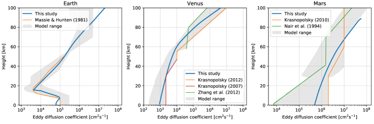
Figure 1: Profiles of eddy diffusion coefficients, $K$ in cm²s^-1 for modern Earth (left panel), Venus (middle panel) and Mars (right panel) calculated with Eq. (1) shown in blue. The $K$ profile of Earth derived from trace gases by Massie & Hunten (1981) is shown in orange. Assumed profiles for Mars in orange from Krasnopolsky (2010a) and in green from Nair et al. (1994). Assumed profiles for Venus are shown in orange from Krasnopolsky (2012), in red from Krasnopolsky (2007) and in green from Zhang et al. (2012). Gray shading indicates range of $K$ for multiple model studies (see text for details).

The eddy diffusion coefficient, $K$, in cm² s^-1 as a function of altitude is assumed analogous to that for heat as derived for free convection by Gierasch & Conrath (1985):

$$K=\frac{H}{3}\left(\frac{L}{H}\right)^{4/3}\left(\frac{R\sigma T^{4}}{\mu\rho C_{\text{p}}}\right)^{1/3},$$ (1)

where $H$ is the scale height, $R$ is the universal gas constant, $\sigma$ is the Stefan-Boltzmann constant, $\mu$ is the atmospheric molecular weight, $\rho$ is the atmospheric density, $C_{\text{p}}$ is the atmospheric heat capacity, and $L$ is the mixing length.

Equation (1) was also used by e.g. Ackerman & Marley (2001) and Gao et al. (2015) to estimate $K$. To fit the $K$ profile of Earth, Mars and Venus we adapt the formula for $L$, which was introduced by Ackerman & Marley (2001):

$$L=\begin{cases}H\cdot\text{max}(0.1,\Gamma/\Gamma_{\text{ad}})&z<z_{\text{ct}}\\ \frac{H_{\text{ct}}}{4}\left(\frac{20}{p_{\text{0}}}+\left(\frac{1}{p}\right)^{1/4}\right)&z\geq z_{\text{ct}}\end{cases},$$ (2)

where $\Gamma$ is the atmospheric lapse rate, $\Gamma_{ad}$ is the adiabatic lapse rate, $p$ is the atmospheric pressure, $p_{\text{0}}$ is the surface pressure, $z_{\text{ct}}$ is the height of the cold trap and $H_{\text{ct}}$ is the scale height at $z_{\text{ct}}$.

For a planet with an ocean, such as Earth, $z_{\text{ct}}$ is the atmospheric layer where water condenses out, i.e. at the lowest layer where $\frac{p_{\text{sat}}}{p}$ starts to increase with height. $p_{\text{sat}}$ is the saturation pressure of water. For a planet without an ocean, such as Mars and Venus, the eddy diffusion can be well described by breaking gravity waves alone (see e.g. Izakov, 2001) and $z_{\text{ct}}$ is set to 0 m.

The left panel of Figure 1 shows the calculated $K$ profile for Earth compared to the $K$ profile derived from trace gases by Massie & Hunten (1981). The gray shaded region represents a range of observational fits from multiple models (Wofsy et al., 1972; Hunten, 1975; Allen et al., 1981). The parametrized values match well the results shown in Massie & Hunten (1981) and lie within the model range except close to the surface, where surface properties can influence transport and towards the upper mesosphere, where e.g. gravity wave breaking can influence mixing and energy budgets. We do not consider a constant eddy diffusion coefficient profile for Earth in the mesosphere and thermosphere as proposed by e.g. Allen et al. (1981) in order to enable the calculation of $K$ to be as general as possible without further assumptions. For most planets $K$ is found to increase towards high altitudes (see e.g. Zhang & Showman, 2018). Note that the model also has the possibility to use a fixed, predefined $K$ profile.

The middle panel of Figure 1 shows reasonable agreement for the calculated $K$ profile of Venus with the assumed profiles from Krasnopolsky (2007), Krasnopolsky (2012) and Zhang et al. (2012). The maximum values of these three studies represent the upper limit of the model range. The lower limit of the model range is taken from Izakov (2001).

The calculated $K$ profile for the Martian atmosphere, compared to the assumed profiles from Krasnopolsky (2010a) and Nair et al. (1994), are shown in the right panel of Figure 1. The lower limit of the model range is from Nair et al. (1994) up to 30 km and from Montmessin et al. (2017) thereabove. The upper limit is from Krasnopolsky (2010a) and Krasnopolsky (2006). Figure 1 shows that the Eq. (1) can represent well the $K$ profiles of Earth, Mars and Venus and hence, is suitable to apply to the scenarios we consider for the TRAPPIST-1 planets.  
 
 

2.4 Model validation

2.4.1 Earth

Table 4: $\Phi_{\text{BOA}}$ and $\Phi_{\text{VOLC}}$ of the Earth in molecules cm^-2 s^-1.

Specie	Anthropogenic	Ref.	Biogenic	Ref.	Volcanic	Ref.	Biogenic and Volcanic
O2	-	-	1.21$\cdot$1012	calc.	-	-	1.21$\cdot$1012
CH4	7.70$\cdot$1010	(1)	6.30$\cdot$1010	(1)	1.12$\cdot$108	(2)	6.31$\cdot$1010
CO	1.16$\cdot$1011	(3)	1.07$\cdot$1011	(3)	3.74$\cdot$108	(2)	1.07$\cdot$1011
N2O	6.58$\cdot$108	(4)	7.80$\cdot$108	(4)	-	-	7.80$\cdot$108
NO	2.46$\cdot$109	(4)	3.38$\cdot$108	(4)	-	-	3.38$\cdot$108
H2S	1.97$\cdot$107	(5)	1.84$\cdot$109	(5)	1.89$\cdot$109	(2)	3.73$\cdot$109
SO2	1.70$\cdot$1010	(5)	-	-	1.34$\cdot$1010	(2)	1.34$\cdot$1010
NH3	3.57$\cdot$109	(6)	8.15$\cdot$108	(6)	-	-	8.15$\cdot$108
OCS	4.54$\cdot$107	(7)	1.39$\cdot$108	(7)	2.67$\cdot$106	(7)	1.42$\cdot$108
HCN	1.32$\cdot$108	(8)	1.27$\cdot$107	(8)	-	-	1.27$\cdot$107
CH3OH	2.91$\cdot$109	(9)	3.35$\cdot$1010	(9)	-	-	3.35$\cdot$1010
CS2	1.15$\cdot$108	(7)	4.98$\cdot$108	(7)	6.23$\cdot$106	(7)	5.05$\cdot$108
CH3Cl	7.97$\cdot$107	(4)	1.39$\cdot$108	(4)	-	-	1.39$\cdot$108
C2H2	9.48$\cdot$108	(8)	-	-	-	-	-
C2H6	7.09$\cdot$108	(4)	8.50$\cdot$108	(10)	5.10$\cdot$106	(10)	8.55$\cdot$108
C3H8	5.52$\cdot$108	(10)	9.49$\cdot$108	(10)	2.29$\cdot$106	(10)	9.51$\cdot$108
HCl	1.32$\cdot$109	(11)	5.13$\cdot$109	(11)	4.42$\cdot$108	(12)	5.57$\cdot$109
H2	7.43$\cdot$1010	(3)	1.86$\cdot$1010	(3)	3.75$\cdot$109	(2)	2.23$\cdot$1010

Note. — The biogenic flux of O₂ corresponds to the value necessary to reproduce a volume mixing ratio of O₂ of 0.21 on modern Earth, assuming a deposition velocity of 1$\cdot$10^-8cm/s. (1) Lelieveld et al. (1998); (2) Catling & Kasting (2017); (3) Hauglustaine et al. (1994); (4) Seinfeld & Pandis (2016); (5) Berresheim et al. (1995); (6) Bouwman et al. (1997); (7) Khalil & Rasmussen (1984); (8) Duflot et al. (2015); (9) Tie et al. (2003); (10) Etiope & Ciccioli (2009); (11) Legrand et al. (2002); (12) Pyle & Mather (2009)

Table 5: $\nu_{\text{dep}}$ as measured for the Earth in cm s^-1.

Specie	$\nu_{\text{dep}}$ (cm s-1)	Reference
O2	1$\cdot$10-8	Arney et al. (2016)
O3	0.4	Hauglustaine et al. (1994)
H2O2	1	Hauglustaine et al. (1994)
CO	0.03	Hauglustaine et al. (1994)
CH4	1.55$\cdot$10-4	Watson (1992)
NO	0.016	Hauglustaine et al. (1994)
NO2	0.1	Hauglustaine et al. (1994)
NO3	0.1	Hauglustaine et al. (1994)
N2O5	4	Hauglustaine et al. (1994)
HNO3	4	Hauglustaine et al. (1994)
HO2NO2	0.4	Hauglustaine et al. (1994)
SO2	1	Sehmel (1980)
NH3	1.7075	Phillips et al. (2004)
OCS	0.01	Seinfeld & Pandis (2016)
CH3OOH	0.25	Hauglustaine et al. (1994)
HCl	0.8	Kritz & Rancher (1980)
HCN	0.044	Duflot et al. (2015)
CH3OH	1.26	Tie et al. (2003)

Note. — For all other species we use $\nu_{\text{dep}}$ of 0.02 cm s^-1, following Hu et al. (2012) and Zahnle et al. (2008).

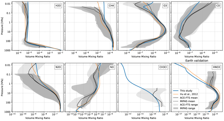
Figure 2: Earth composition profiles for selected species predicted with our photochemistry model shown in blue, compared to the results from Hu et al. (2012) in orange and to MIPAS and ACE-FTS measurements in black. Dark gray shaded regions indicate MIPAS measurement ranges whereas light gray shaded regions indicate ACE-FTS measurement ranges (see text for details).

We first validate our model by simulating the modern Earth around the Sun and comparing the results with observations from measurements of the Michelson Interferometer for Passive Atmospheric Sounding (MIPAS; Fischer et al., 2008) and the Atmospheric Chemistry Experiment Fourier Transform Spectrometer (ACE-FTS; Bernath, 2017). Details of the MIPAS and ACE-FTS data processing can be found in von Clarmann et al. (2009) and Boone et al. (2005) respectively. The references of the individual datasets for each species can be found on the MIPAS web page and the ACE-FTS web page .

We select only the data with high quality, determined as following. For MIPAS data we follow the recommendations that the diagonal element of the averaging kernel needs to be at least 0.03 and the visibility flag must be unity . The ACE-FTS data contains a quality flag indicating physically unrealistic outliers (Sheese et al., 2015). The selected data is averaged for each satellite flyover onto a grid with a resolution of 5^∘ in latitude by 10^∘ in longitude. We repeat this step for each available observation. We take into account 95% of the data and exclude the 5% extremes. The maximum and minimum value for each altitude level represents the measured range shown as gray shading in Figure 2. To calculate the global and annual mean profile of each specie we calculate a monthly mean and from that an annual mean at each grid point. This ensures that each season of the year is equally represented. Finally we average over the grid with a zonal and weighted meridional mean.

Different to our previous studies we do not tune the surface fluxes to reproduce the observed surface abundances of CO, NO₂, CH₄ and CH₃Cl (e.g. Grenfell et al., 2013, 2014; Wunderlich et al., 2019). Instead we use the sum of observed anthropogenic, biogenic and volcanic surface fluxes (see Table 4) and observed $\nu_{\text{dep}}$ (see Table 5). Also included are modern-day tropospheric lightning emissions of NO_x. We apply an upper boundary condition for H and H₂ with the parametrization from Hu et al. (2012). To simulate modern Earth we use the solar spectrum from Gueymard (2004). The temperature profile simulated with the model is shown in the companion paper (Scheucher et al., accepted). To achieve a mean surface temperatures of 288.15 K in our cloud-free model we use a surface albedo of 0.255.

Figure 2 shows that the photochemistry of the Earth can be reproduced well with the new chemical network. We also compare well to the results shown by Hu et al. (2012). Tropospheric abundances of all shown species lie within the measurement range. In the upper stratosphere and mesosphere the abundances of HNO₃ are underestimated in both models compared to measurements. This discrepancy could be due to missing NO_x-related processes, such as energetic particle precipitation, producing NO_x in the upper mesosphere and subsequent dynamical transport into the stratosphere (see e.g. Krivolutsky, 2001; Siskind et al., 2000; López-Puertas et al., 2005; Clilverd et al., 2009; Funke et al., 2005, 2010, 2014, 2016).

2.4.2 Mars

As a second validation case we simulate the atmosphere of modern Mars. We use the atmospheric temperature profile from Haberle et al. (2017), representing a scenario with weak dust loading. The data is based on diurnal averages of Mars Climate Sounder (MCS) observations (Kleinböhl et al., 2009). The radiative-convective climate module is not used here to calculate the temperature profile since we want to focus on the validation of the photochemistry model. The climate validation for Mars is presented in Scheucher et al. (accepted). The mean surface pressure of the reference atmosphere is 5.62 hPa (Haberle et al., 2017). We use a bond albedo of 0.25 (Williams, 2010). The eddy diffusion coefficients are directly calculated in the model (see Section 2.3.3).

In Table 6 we show the boundary conditions used to model the Martian atmosphere. N₂ serves as a fill gas and is 2.82% over the entire atmosphere, which is similar to the measurements of Owen et al. (1977) which suggested a volume mixing ratio of 2.7%.

Table 6: Boundary conditions of modern Mars.

Specie	Lower	Ref.	Upper	Ref.
CO2	$f$ = 0.9532	(1)	$\Phi_{\text{TOA}}$ = 0	-
H2O	$f$ = 3$\cdot$10-4	(1)	$\Phi_{\text{TOA}}$ = 0	-
CH4	$\Phi_{\text{BOA}}$ = 7.5$\cdot$103	(2)	$\Phi_{\text{TOA}}$ = 0	-
SO2	$\Phi_{\text{BOA}}$ = 1.5$\cdot$106	(3)	$\Phi_{\text{TOA}}$ = 0	-
HCl	$\Phi_{\text{BOA}}$ = 2.4$\cdot$104	(4)	$\Phi_{\text{TOA}}$ = 0	-
H2	$\Phi_{\text{BOA}}$ = 0	-	$\nu_{\text{eff}}$ = 3.39	(5)
H	$\Phi_{\text{BOA}}$ = 0	-	$\nu_{\text{eff}}$ = 3080	(6)
O	$\Phi_{\text{BOA}}$ = 0	-	$\Phi_{\text{TOA}}$ = 1$\cdot$107	(7)
O2	$\nu_{\text{dep}}$ = 1$\cdot$10-8	(8)	$\Phi_{\text{TOA}}$ = 0	-
CO	$\nu_{\text{dep}}$ = 1$\cdot$10-8	(9)	$\Phi_{\text{TOA}}$ = 0	-
other	$\nu_{\text{dep}}$ = 2$\cdot$10-2	(7)	$\Phi_{\text{TOA}}$ = 0	-

Note. — See Section 2.3 for description of how the boundaries are included in the model. $\Phi_{\text{BOA}}$ and $\Phi_{\text{TOA}}$ are in molecules cm^-2 s^-1, $\nu_{\text{dep}}$ and $\nu_{\text{eff}}$ are in cm s^-1. Following Zahnle et al. (2008), for all species not listed here we assume a $\nu_{\text{dep}}$ of 0.02 cm s^-1. (1) Owen et al. (1977), (2) $\Phi_{\text{BOA}}$ necessary to fit the mean surface value of $f_{\text{CH${}_{4}$}}$ = 4$\cdot$10^-10 (Webster et al., 2018), (3) $\Phi_{\text{BOA}}$ necessary to fit the upper limit of $f_{\text{SO${}_{2}$}}$ = 3$\cdot$10^-10 (Encrenaz et al., 2011), (4) $\Phi_{\text{BOA}}$ necessary to fit the upper limit of $f_{\text{HCl}}$ = 2$\cdot$10^-10 (Hartogh et al., 2010), (5) $\nu_{\text{eff}}$ necessary to fit $f_{\text{H${}_{2}$}}$ = 1.5$\cdot$10^-5 at TOA (Krasnopolsky & Feldman, 2001); Nair et al. (1994) used $\nu_{\text{eff}}$ = 33.9  cm s^-1, (6) Nair et al. (1994), (7) Zahnle et al. (2008), (8) Arney et al. (2016), (9) Kharecha et al. (2005). We use a constant volume mixing ratio of argon profile of 1.6% (Owen et al., 1977). N₂ serves as a fillgas.

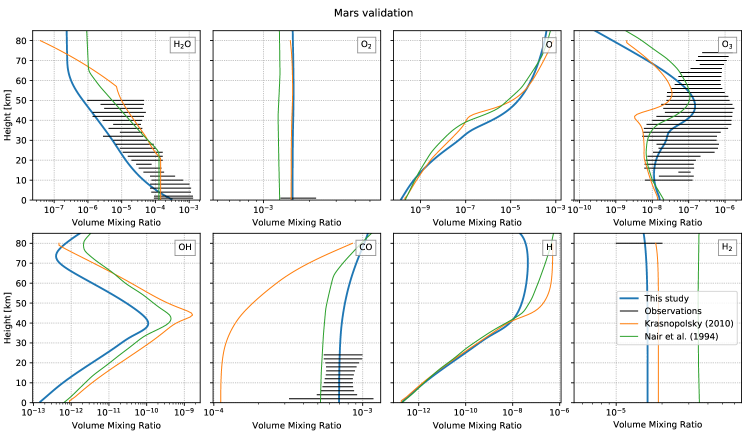
Figure 3: Mars composition profiles for selected species predicted with our photochemistry model shown in blue, compared to the results from Krasnopolsky (2010a) in orange, Nair et al. (1994) in green and a range of multiple observations in black (see text for details).

Figure 3 shows the profile of selected atmospheric species compared to the model results of Krasnopolsky (2010a) and the following measurements. For H₂O we take into account Mars Express PFS (Planetary Fourier Spectrometer) nadir measurements up to 30 km from Montmessin & Ferron (2019) and SPICAM (Spectroscopy for the Investigation of the Characteristics of the Atmosphere of Mars) measurements above 20 km from Fedorova et al. (2009). O₃ ranges are taken from nighttime and sunrise/sunset measurements (Montmessin & Lefèvre, 2013; Lebonnois et al., 2006). CO observational ranges are taken from retrieval uncertainties around 800 ppm from PFS/Mars Express infrared nadir observations (Bouche et al., 2019). The H₂ range at 80 km is given in Krasnopolsky & Feldman (2001) and O₂ range at the surface is taken from Trainer et al. (2019). We compute the observational ranges by finding the lowest and highest value in a 2 km grid from measured profiles or observations of the mixing ratio at a given altitude. Note that surface values are located at 1 km for visibility purposes.

The Martian atmosphere simulated with the photochemistry model compares well with the results from Krasnopolsky (2010a) and Nair et al. (1994). The model simulates H₂O abundances close to the lower minimum of measured concentrations. When using an eddy diffusion flux increased by a factor of ten, more water is transported upwards and the modelled H₂O abundances fit to the measurements (not shown). Since we model an aerosol free atmosphere the low H₂O content is consistent with observations of Vandaele et al. (2019) showing increased atmospheric H₂O during dust storms. Note that Krasnopolsky (2010a) and Nair et al. (1994) used a predefined H₂O profile while we calculate the H₂O profile consistently in the photochemical model. The underestimation of the O₃ content above 60 km may be related to diurnal changes in the solar zenith angle, not included in the model. We obtain a surface O₂ concentration of 1552 ppm which is consistent with the global mean of 1560$\pm$54 ppm inferred by Krasnopolsky (2017) and also in the range of the seasonal variation of O₂ (1300 - 2200 ppm, Trainer et al., 2019).

In summary we show that our photochemistry model gives consistent results compared to previous photochemistry models and observations of the Martian atmosphere. Different from many previous models, we also simulate consistently the chemistry of chlorine, sulphur and methane. The emission fluxes required to reproduce observations of CH₄, HCl and SO₂ are shown in Table 6. The Martian CH₄ chemistry will be discussed in detail in a follow up paper by Grenfell et al. (in prep).

2.4.3 Venus

Table 7: Boundary conditions of modern Venus.

Specie	Lower	Ref.
CO2	$f$ = 0.965	Zhang et al. (2012)
CO	$\nu_{\text{m}}=0.1K/H$	Krasnopolsky (2012)
H2O	$f$ = 4.0$\cdot$10-6	tuned
OCS	$f$ = 1.2$\cdot$10-8	tuned
NO	$f$ = 5.5$\cdot$10-9	Zhang et al. (2012)
HCl	$f$ = 1$\cdot$10-6	tuned (calc. edd. diff.)
HCl	$f$ = 4$\cdot$10-7	Zhang et al. (2012) (K12 edd. diff.)
SO2	$f$ = 3.5$\cdot$10-6	Zhang et al. (2012)
other	$\nu_{\text{m}}=K/H$	Zhang et al. (2012)

Note. — For all species not listed here we assume a maximum deposition velocity $\nu_{\text{m}}=K/H$, using $K$ and $H$ at 58 km to take into account that our BoA is not the surface (see Zhang et al., 2012; Krasnopolsky, 2012). $f_{\text{HCl}}$ = 1$\cdot$10^-6 for the run with a calculated $K$ and $f_{\text{HCl}}$ = 4$\cdot$10^-7 for the run with $K$ taken from Krasnopolsky (2012). N₂ serves as fillgas.

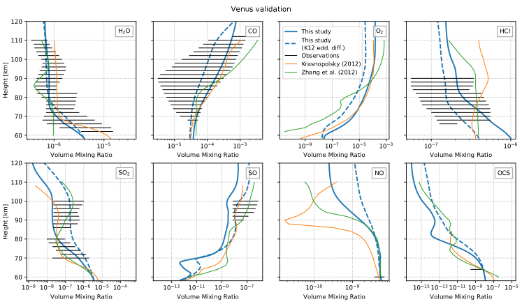
Figure 4: Venus composition profiles for selected species predicted with our photochemistry model with calculated $K$ (solid blue line) and with $K$ taken from Krasnopolsky (2012) with breakpoint $h_{\text{e}}$ at 65 km (K12 edd. diff., dashed blue line), compared to the results from Krasnopolsky (2012), Zhang et al. (2012) and a range of observations inferred from multiple studies (see text for details).

Predicting the atmospheric composition of Venus is challenging since details of the sulphur chemistry are not understood completely (e.g. Mills & Allen, 2007; Zhang et al., 2012; Vandaele et al., 2017). The atmospheric chemistry of Venus below and above the cloud deck is usually modeled separately. We validate our model by calculating the atmosphere of Venus only in the photochemical regime above the cloud top at $\sim$58 km, where direct observations of chemical species are available. The temperature profile is taken from the Venus International Reference Atmosphere VIRA-1 (Seiff et al., 1985).

The boundary conditions are presented in Table 7. Following Zhang et al. (2012) and Krasnopolsky (2012) we use fixed volume mixing ratios at BoA for key species to fit the observed values and we assume a downward flux of all other species depending on $K$ and $H$ (see also Section 2.3.3). Figure 4 shows the profiles of the species with existing observations and profiles taken from Zhang et al. (2012) and Krasnopolsky (2012).

The range of observational values is derived by combining multiple studies. The H₂O range is generated by combining measurements from Bertaux et al. (2007) and measurements shown in Figure 3 of Krasnopolsky (2012). CO measurements are taken from Svedhem et al. (2007) and Figure 2 of Krasnopolsky (2012). HCl measurements are taken from Sandor & Clancy (2012) and Bertaux et al. (2007). For the observational range of SO₂ and SO we use Venus Express solar occultations in the infrared range and SPICAV (Spectroscopy for Investigation of Characteristics of the Atmosphere of Venus) occultations from Belyaev et al. (2012) and submillimeter measurements from Sandor et al. (2010). The OCS observation is taken from Krasnopolsky (2010b) and NO measurements from Krasnopolsky (2006). As for the Mars validation we compute the observational ranges by finding the lowest and highest value in a 2 km grid.

We find that our model is able to reproduce the Venus atmosphere above 58 km and leads to broadly comparable results as for other photochemical models. Our model reproduces the measurements best with a H₂O mixing ratio of 4.0$\cdot$10^-6, which is in between the values shown in Krasnopolsky (2012) and Zhang et al. (2012). The HCl profile of our model is consistent with the decrease between 70 and 100 km found by observations (Sandor & Clancy, 2012) and was not reproduced by the models of Krasnopolsky (2012) and Zhang et al. (2012). On using our calculated eddy diffusion coefficients we underestimate the abundances of SO₂ and SO between 90 and 100 km. Using larger eddy diffusion coefficients from Krasnopolsky (2012) we then lie in the observational range of SO₂ and SO between 90 and 100 km but slightly overestimate the SO₂ abundances around 80 km. This degeneracy may be caused by the missing consideration of sulphur hazes in the upper atmosphere (see e.g. Gao et al., 2014).

In summary we find that we can predict the upper atmosphere of Venus similarly well as other models, even without consideration of the effect of hazes above the cloud layer.

2.5 Transmission spectra

The climate-photochemistry model is used to simulate atmospheric temperature and composition profiles of potential atmospheres of TRAPPIST-1 e and TRAPPIST-1 f. With the resulting profiles we produce transmission spectra of the planetary atmospheres using the ”Generic Atmospheric Radiation Line-by-line Infrared Code” (GARLIC; Schreier et al., 2014, 2018). GARLIC has been used in recent exoplanet studies such as Scheucher et al. (2018); Katyal et al. (2019); Wunderlich et al. (2019).

We simulate transmission spectra including 28 atmospheric species between 0.4 $\mu$m and 12 $\mu$m. Line parameters are taken from the HITRAN 2016 database (Gordon et al., 2017) and the Clough-Kneizys-Davies (CKD) continuum model (Clough et al., 1989). Additionally Rayleigh extinction is considered (Murphy, 1977; Clough et al., 1989; Sneep & Ubachs, 2005; Marcq et al., 2011). In the visible we use the cross sections at room temperature (298 K) for O₃, NO₂, NO₃ and HOCl listed in Table 3.

For the 1D climate-photochemistry simulations we do not consider cloud formation. Hence, all the transmission spectra we calculate in this study show cloud-free conditions. However, an Earth-like extinction from uniformly distributed aerosols in the atmosphere can be considered in GARLIC. The aerosol optical depth, $\tau_{\text{A}}$, at wavelength $\lambda$ ($\mu$m) is expressed following Ångström (1929, 1930):

$$\tau_{\text{A}}=\beta\cdot\lambda^{-\alpha},$$ (3)

assuming that the aerosol size distribution follows the Junge distribution (Junge, 1952, 1955). For the exponent, $\alpha$, we use 1.3, representing the average measured value on Earth (see e.g. Ångström, 1930, 1961). The Ångström turbidity coefficient, $\beta$, is expressed using the cross section data for the Earth’s atmosphere taken from Allen (1976):

$$\beta=1.4\cdot 10^{-27}\cdot N_{\text{c}},$$ (4)

where $N_{\text{c}}$ is the column density in molecules cm^-2 (see also Toon & Pollack, 1976; Kaltenegger & Traub, 2009; Yan et al., 2015). According to Allen (1976) the Eq. (4) corresponds to clear atmospheric conditions with weak scattering by haze or dust.

The transmission spectra from GARLIC are expressed as effective heights:

$$h_{\text{e}}(\lambda)=\int_{0}^{ToA}\Big{(}1-\mathcal{T}(\lambda,z)\Big{)}~{}dz,$$ (5)

where $\mathcal{T}$ is the transmission along the limb with the tangent altitude, $z$. $h_{\text{e}}$ is the integration over all $\mathcal{T}$ from the surface to the top of atmosphere (ToA) at each wavelength, $\lambda$. The measured transit depth, $t_{\text{depth}}$, of a planet with an atmosphere is the sum of the planet radius, $R_{\text{p}}$, and $h_{\text{e}}$ with respect to the stellar radius, $R_{\text{s}}$. The atmospheric transit depth, $t_{\text{atm}}$, only contains the contribution of the atmosphere to the total transit depth:

$$t_{\text{atm}}(\lambda)=\frac{(R_{\text{p}}+h_{\text{e}}(\lambda))^{2}}{R_{\text{s}}^{2}}-\frac{R_{\text{p}}^{2}}{R_{\text{s}}^{2}}.$$ (6)

In order to detect a spectral feature we make use of the wavelength dependence of $t_{\text{atm}}$. To extract the measurable atmospheric signal, $S_{\text{atm}}$, we subtract the minimum atmospheric transit depth, $t_{\text{min}}$, in the considered wavelength range (baseline) from the $t_{\text{atm}}$ at each wavelength point:

$$t_{\text{min}}=\min{(t_{\text{atm}}(\lambda))},$$ (7)

$$S_{\text{atm}}(\lambda)=t_{\text{atm}}(\lambda)-t_{\text{min}}.$$ (8)

The wavelength dependent $S_{\text{atm}}$, expressed as parts per million (ppm), is used to calculate the signal-to-noise ratio (S/N) of molecular features. Taking into account the $h_{\text{e}}(\lambda)$ instead would overestimate the S/N of the spectral features, because that measure would include the continuum extinction.

2.6 Signal-to-noise ratio (S/N)

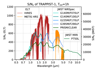
Figure 5: Stellar S/N of TRAPPIST-1 for 1 h integration time and binned to a resolving power of $R$=100,000 for ELT (left y-axis) and a $R$=30 for JWST (right y-axis). The conversion factor from the right to the left y-axis is $\sqrt{\frac{100,000}{30}}$, corresponding to a white noise binning of the S/N_s. The stellar S/N of JWST is the combination of all NIRSpec filter and disperser and MIRI LRS, calculated with the method presented in Wunderlich et al. (2019). We do not consider a partial saturation strategy as suggested by Batalha et al. (2018). The stellar S/N of ELT is calculated with the ESO ETC Version 6.4.0 (Liske, 2008).

Table 8: Wavelength coverage and resolving power, $R$, of the instruments on JWST and ELT used to calculate SNR_s of TRAPPIST-1.

Telescope	Instrument	Wavelength	$R$	Reference
JWST	NIRSpec PRISM/CLEAR	0.6 - 5.3 $\mu$m	$\sim$100	Birkmann et al. (2016)
JWST	NIRSpec G140M/F070LP	0.7 - 1.27 $\mu$m	$\sim$1,000	Birkmann et al. (2016)
JWST	NIRSpec G140M/F100LP	0.97 - 1.84 $\mu$m	$\sim$1,000	Birkmann et al. (2016)
JWST	NIRSpec G235M/F170LP	1.66 - 3.07 $\mu$m	$\sim$1,000	Birkmann et al. (2016)
JWST	NIRSpec G395M/F290LP	2.87 - 5.10 $\mu$m	$\sim$1,000	Birkmann et al. (2016)
JWST	MIRI P750L (LRS)	5.0 - 12 $\mu$m	$\sim$100	Kendrew et al. (2015)
ELT	HIRES	0.37 - 2.5 $\mu$m	100,000	Marconi et al. (2016)
ELT	METIS (HRS)	2.9 - 5.3 $\mu$m	100,000	Brandl et al. (2016)

We determine which atmospheric spectral features of the simulated atmospheres of TRAPPIST-1 e and TRAPPIST-1 f could be detectable with ELT and JWST. Lustig-Yaeger et al. (2019) showed that the S/N for emission spectroscopy of TRAPPIST-1 e and TRAPPIST-1 f is too low to detect spectral features (see also Batalha et al., 2018). Hence, we limit our analysis to transmission spectroscopy.

To calculate the S/N of planetary atmospheric feature, S/N${}_{\text{atm}}$, of a single transit, we first calculate the S/N of the star, S/N${}_{\text{s}}$, integrated over one transit and then multiply this value with $S_{\text{atm}}$:

$$\text{S/N}_{\text{atm}}=\frac{S_{\text{atm}}}{\sqrt{2}}\cdot\text{S/N}_{\text{s}}.$$ (9)

The factor $\frac{1}{\sqrt{2}}$ accounts for the fact that the star is observed during in transit and out of transit. We calculate the number of transits, $n_{\text{tr}}$, necessary to reach an S/N of 5, assuming that all transits improve S/N${}_{\text{s}}$ perfectly. The S/N${}_{\text{s}}$ for JWST NIRSpec and MIRI is determined by the method and instrument specifications presented in Wunderlich et al. (2019) (see Table 8 for the wavelength coverage and resolving power, $R=\frac{\lambda}{\Delta\lambda}$).

The S/N${}_{\text{s}}$ of the ELT High Resolution Spectrograph (HIRES; Marconi et al., 2016) is calculated with the ESO Exposure Time Calculator (ETC) Version 6.4.0 from November 2019 (see updated documentation from Liske, 2008). The ETC uses the background sky model for the Cerro Paranal and considers photon and as well as detector noises such as readout noise and dark current. The ETC assumes a spectrograph with a throughput of 25%, independent of the resolving power. For HIRES or METIS HRS this value might overestimate the real value. For METIS HRS the expected throughput ranges between 6% and 21% (Cárdenas Vázquez, personal communication). Hence, we scale down the S/N${}_{\text{s}}$ for both instruments to an average throughput of 10%.

We assume a telescope with a diameter of 39 m at Paranal in Chile (2,635 m). The planned location of the ELT at Cerro Armazones (3,046 m) is not available in the ETC. The sky conditions are set to a constant airmass of 1.5 and a precipitable water vapour (PWV) of 2.5 (Liske, 2008). The ETC does not provide the possibility to choose the individual ELT instrumentations but we consider the wavelength coverage and $R$ for the instruments planned for the ELT (see Table 8). For each wavelength band we change the radius of the diffraction limited core of the point spread function according to the recommendation in the ETC manual. The wavelengths from 2.9 $\mu$m to 3.4 $\mu$m cannot be calculated by the current version of the ETC.

To simulate an observation of TRAPPIST-1 we scale the stellar spectrum from Wilson et al. (submitted) to the J-band magnitude of 11.35 (Gillon et al., 2016) in order to obtain the input flux distribution.

The S/N${}_{\text{s}}$ for a one hour integration of TRAPPIST-1 for JWST and ELT is shown in Figure 5. The ground-based facility ELT will have a much larger telescope area compared to the space-borne JWST but its capability of detecting spectral features with low resolution spectroscopy is limited to atmospheric windows with minor telluric contamination. However, high-resolution spectra ($R$ $>$ 25,000) resolve individual lines improving their detectability. The Doppler-shift of the lines during the transit with respect to the absorption lines of the Earth’s atmosphere is measurable for close-in planets (see e.g. Birkby, 2018). Previous theoretical and observational studies have shown that a detection of molecules such as O₂, H₂O or CO is feasible via cross-correlation (e.g. Snellen et al., 2013; Birkby et al., 2013; Brogi et al., 2018; Mollière & Snellen, 2019; López-Morales et al., 2019; Sánchez-López et al., 2019).

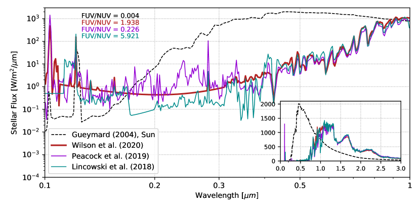
Figure 6: Input stellar spectral energy distribution (SED) of TRAPPIST-1 and the Sun. Red line: TRAPPIST-1 SED with the UV estimated with a semi-empirical model using HST observational data provided by the Mega-MUSCLES survey (Wilson et al., submitted), marked W20 SED. Cyan line: TRAPPIST-1 SED with estimated UV flux by scaling the spectrum of Proxima Centauri (Lincowski et al., 2018), marked L18 SED. Violet line: TRAPPIST-1 SED with calculated UV flux using a semi-empirical non-LTE model Peacock et al. (2019), marked P19 SED. Black line: solar SED taken from Gueymard (2004). For the FUV/NUV ratio the FUV is integrated between 117-175 nm and the NUV is integrated over 175-320 nm (see Tian et al., 2014).

We adopt a simple approach in order to estimate the number of transits which are necessary to detect e.g. O₂, H₂O and CO with the cross-correlation method in our simulated atmospheres. We adapted a formula presented in Snellen et al. (2015) to calculate the signal-to-noise ratio of the planet, considering the wavelength dependency of $S_{\text{atm}}$ and S/N${}_{\text{s}}$

$$\text{S/N}_{\text{atm}}=\frac{\sum_{l=0}^{n_{\text{l}}}S_{\text{atm}}(\lambda_{\text{l}})\cdot S/N_{\text{s}}(\lambda_{\text{l}})}{n_{\text{l}}}\cdot\sqrt{t_{\text{int}}}\cdot\sqrt{n_{\text{l}}},$$ (10)

where $n_{\text{l}}$ is the number of spectral lines and $t_{\text{int}}$ is the integration time. $t_{\text{int}}$ is calculated by $t_{\text{dur}}\cdot n_{\text{tr}}$, with the transit duration, $t_{\text{dur}}$, and the number of transits, $n_{\text{tr}}$. The S/N${}_{\text{s}}$ at the wavelength of the line, $\lambda_{\text{l}}$, used in Eq. (10), is the S/N${}_{\text{s}}$ shifted by one bandwidth to account for the displacement of the spectral line during transit.

Using Eq. (10) we find that a 3$\sigma$ detection of O₂ on an Earth-twin around an M7 star at a distance of 5 pc might be feasible when co-adding 58 transit observations in the J-band with ELT HIRES, assuming a throughput of 20%. Rodler & López-Morales (2014) suggested that 26 transits are needed to detect O₂ when using the same assumptions.

Section 4.5.6 discusses the detectability of the CO spectral feature in the atmosphere of a hypothetical planets around other low mass stars in the solar neighbourhood. For stars on the Northern sky we calculate the S/N${}_{\text{s}}$ for the Thirty Meter Telescope (TMT, Nelson & Sanders, 2008). This will have a smaller telescope area than the ELT but will be located at a higher altitude of 4,064 m, compared to 2,635 m at Paranal. Hence, due to the lower PWV and weaker high-altitude turbulence at Mauna Kea the TMT is expected to have a similar performance as the ELT. We compare the S/N_s of ELT with $R$=4,000 at a Vega magnitude of 16 in the J-band to calculation of the S/N_s with the same specifications using the Infrared Imaging Spectrograph (IRIS) on TMT by Wright et al. (2014) and find that ELT has a 10% lower S/N_s than TMT.

Since the performance of the telecopes during operation is not yet established we simply assume that the TMT provides the same S/N_s as the ELT.

3 Stellar input and model scenarios

3.1 TRAPPIST-1 spectra

The Spectral Energy Distribution (SED) in the UV has a large impact on the photochemisty of atmospheres of terrestrial planets (see e.g. Selsis et al., 2002; Grenfell et al., 2013, 2014; Tian et al., 2014). In this study we use the semi-empirical model spectrum of TRAPPIST-1 from Wilson et al. (submitted), which we will refer to as W20 SED. The constructed SED uses observational data from XMM-Newton for the X-ray regime and from the Hubble Space Telescope (HST) for the 113 to 570 nm range with a gap between 208-279 nm obtained through the Mega-MUSCLES Treasury survey (Froning et al., 2018). The wavelengths larger than 570 nm are filled by Wilson et al. (submitted) with a PHOENIX photospheric model (Allard, 2016; Baraffe et al., 2015).

Figure 6 compares the Mega-MUSCLES TRAPPIST-1 SED with spectra, presented in previous studies. Lincowski et al. (2018) estimated the UV radiation of TRAPPIST-1 by scaling the Proxima Centauri’s spectrum to the Ly$\alpha$ measurements of TRAPPIST-1 from Bourrier et al. (2017), in the following referred to as L18 SED. Peacock et al. (2019) present a semi-empirical non-local thermodynamic equilibrium (non-LTE) model spectrum of TRAPPIST-1, based on the stellar atmosphere code PHOENIX (Hauschildt, 1993; Hauschildt & Baron, 2006; Baron & Hauschildt, 2007), here referred to as P19 SED.

We bin all spectra into 128 bands for the climate model and 133 bands for the photochemistry model. The spectra for TRAPPIST-1, as well as the solar spectrum from Gueymard (2004) are shown in Figure 6. All SEDs are scaled to an integrated total energy of 1361 W/m² which is equal to the energy the Earth receives from the Sun.

Table 9: Planetary parameters used as input for the climate-photochemistry model and to calculate the S/N of spectral features. The planetary radii from Delrez et al. (2018a) are corrected according to Kane (2018). The gravity is calculated using given planetary mass and radius.

Planets	e	f	Reference
Radius ($R_{\earth}$)	0.94	1.08	Kane (2018)
Mass ($M_{\earth}$)	0.772	0.934	Grimm et al. (2018)
Gravity (m/s2)	8.56	7.85	-
Irradiation (S☉)	0.604	0.349	Delrez et al. (2018a)
Transit duration (min)	55.92	63.14	Delrez et al. (2018a)
Impact parameter $b$ ($R_{*}$)	0.24	0.337	Delrez et al. (2018a)

Note. — Using the updated stellar parameters from Kane (2018) the planetary radii are $\sim$3 larger and the gravities $\sim$7 lower than the values used by previous studies such as Lincowski et al. (2018).

Table 10: Mean surface temperature predicted with our 1D climate model (see Scheucher et al., accepted) for different main atmospheric compositions and stellar irradiations of TRAPPIST-1 e and TRAPPIST-1 f (T${}_{\text{1D}}$). S${}_{\text{D18}}$ corresponds to the irradiation values shown in Delrez et al. (2018a) and S${}_{\text{G17}}$ corresponds to the values taken from Gillon et al. (2017). The surface temperatures predicted with various 3D models are shown for comparison (T${}_{\text{3D}}$). The last column shows the reference of the corresponding 3D model study.

Planet	CO2 (bar)	N2 (bar)	CH4 (bar)	T${}_{\text{1D}}$ (S${}_{\text{D18}}$)	T${}_{\text{1D}}$ (S${}_{\text{G17}}$)	T${}_{\text{3D}}$ (S${}_{\text{G17}}$)	Ref.
e	0.01	1	0	253	262	254	(1)
e	0.1	1	0	269	279	273	(1)
e	1	1	0	328	337	331	(1)
e	0	1	0.01	223	231	211	(2)
e	1	0	0	303	312	303	(3)
e	10	0	0	392	401	392	(3)
f	1	0	0	222	229	230	(3)
f	10	0	0	321	334	350	(3)

Note. — (1) Wolf (2017), (2) Turbet et al. (2018), (3) Fauchez et al. (2019)

Table 11: Scenarios assumed as input for the climate-photochemistry model to simulate the atmosphere of TRAPPIST-1 planets. The relative humidity (RH) is assumed to be constant up to the cold trap. The surface fluxes are the same as for pre-industrial Earth (see Table 4). For wet & alive and wet & dead we assume $\nu_{\text{dep}}$ for O₂ and CO according to the underlying scenario. For all other species the $\nu_{\text{dep}}$ shown in Table 5 are used. For each scenario we assume a range of CO₂ surface partial pressures. N₂ serves as a fill gas to reach the assumed surface pressure, p₀.

Scenario	Planet	CO2 (bar)	$p_{0}$ (bar)	RH	Surface flux	O2 $\nu_{\text{dep}}$ (cm s-1)	CO $\nu_{\text{dep}}$ (cm s-1)
Wet & alive	TRAPPIST-1 e	10-3	1.001	80%	Biogenic and Volcanic (see Table 4)	1$\cdot$10-8	3$\cdot$10-2 (1$\cdot$10-8)
	TRAPPIST-1 e	0.01	1.01
	TRAPPIST-1 e	0.1	1.1
	TRAPPIST-1 e	1.0	2.0
	TRAPPIST-1 f	3.6	4.0
	TRAPPIST-1 f	10.8	12.0
Wet & dead	TRAPPIST-1 e	10-3	1.001	80%	Volcanic (see Table 4)	1.5$\cdot$10-4 (1$\cdot$10-8)	1.2$\cdot$10-4 (1$\cdot$10-8)
	TRAPPIST-1 e	0.01	1.01
	TRAPPIST-1 e	0.1	1.1
	TRAPPIST-1 e	1.0	2.0
	TRAPPIST-1 f	3.6	4.0
	TRAPPIST-1 f	10.8	12.0
Dry & dead	TRAPPIST-1 e	10-3	1.001	80%	Volcanic (see Table 4)	1$\cdot$10-8	1$\cdot$10-8
	TRAPPIST-1 e	0.01	1.01
	TRAPPIST-1 e	0.1	1.1
	TRAPPIST-1 e	1.0	2.0
	TRAPPIST-1 f	3.6	4.0
	TRAPPIST-1 f	10.8	12.0

Note. — CO₂-poor atmosphere of TRAPPIST-1 e with CO₂ partial pressures of only 10^-3 and 0.01 bar correspond to a $T_{\text{surf}}$ for the wet & alive run of about 250 K and 260 K, respectively. CO₂ partial pressures of 0.1 bar and 3.6 bar for TRAPPIST-1 e and TRAPPIST-1 f, respectively, correspond to a $T_{\text{surf}}$ of about 273 K for the wet & alive run. CO₂ partial pressures of 1 bar and 10.8 bar for TRAPPIST-1 e and TRAPPIST-1 f, respectively, correspond to a $T_{\text{surf}}$ of about 340 K for the wet & alive run.

O₂ deposition is 1$\cdot$10^-8 for an ocean saturated with O₂ (wet & alive) and for dry & dead conditions without effective O₂ surface sinks (Arney et al., 2016). For wet & dead conditions we assume that the ocean is either saturated or the ocean takes up the O₂ with a $\nu_{\text{dep}}$ of 1.5$\cdot$10^-4 cm s^-1 (Domagal-Goldman et al., 2014; Catling & Kasting, 2017). Schwieterman et al. (2019) used a similar value of $\nu_{\text{dep}}$ = 1.4$\cdot$10^-4 cm s^-1 for anoxic atmospheres.

For wet & alive conditions we assume the same CO deposition of $\nu_{\text{dep}}$ = 3$\cdot$10^-2 cm s^-1 as on Earth (Hauglustaine et al., 1994; Sanhueza et al., 1998), which is larger than the $\nu_{\text{dep}}$ of 1.2$\cdot$10^-4 cm s^-1 calculated for anoxic wet atmospheres (Kharecha et al., 2005; Domagal-Goldman et al., 2014; Catling & Kasting, 2017; Schwieterman et al., 2019). For conditions without effective CO surface sinks we use a $\nu_{\text{dep}}$ of 1$\cdot$10^-8 cm s^-1 (Kharecha et al., 2005; Hu et al., 2020).

3.2 System parameters and habitability

We use the following stellar parameters of TRAPPIST-1: a $T_{\text{eff}}$ of 2516 K (Van Grootel et al., 2018), a radius of 0.124 $R_{\sun}$ (Kane, 2018), a mass of 0.089 $M_{\sun}$ (Van Grootel et al., 2018) and a distance of 12.43 pc (Kane, 2018). Table 9 provides the planetary parameters for planet e and f used to model the atmosphere and to calculate the S/N of the produced transmission spectra. We do not focus here on TRAPPIST-1 g since initial studies with our model (not shown) suggested cold, non-habitable conditions, even assuming several tens of bar of surface CO2, although this is a subject for future study (see e.g. Wolf, 2017; Turbet et al., 2018; Lincowski et al., 2018).

Most previous studies used the planetary parameters from Gillon et al. (2017) with an irradiation of 0.662 S_☉ for TRAPPIST-1 e and an irradiation of 0.382 S_☉ for planet f. In Table 10 we compare the mean surface temperature for different atmospheric compositions and using the irradiation from Gillon et al. (2017) and Delrez et al. (2018a). We also compare the temperatures with results from 3D studies.

1D models have difficulties to simulate the atmosphere of planets orbiting low-mass stars in synchronous rotation self-consistently (see e.g. Yang et al., 2013; Leconte et al., 2015; Barnes, 2017). However, Table 9 shows that the surface temperatures predicted with our 1D model are in general agreement with the results from 3D studies. Using the stellar irradiation from Gillon et al. (2017) we overestimate the temperatures by $\sim$10 K for TRAPPIST-1 e. Only for the Titan-like atmosphere with 0.01 bar CH₄ and 1 bar N₂ do we predict a larger difference of 20 K. For a 10 bar CO₂ atmosphere of TRAPPIST-1 f we obtain a 16 K lower surface temperature compared to Fauchez et al. (2019). Note that we only simulate cloud-free conditions. The consideration of clouds in 1D models would likely but not always lead to a lower surface temperature (see e.g. Kitzmann et al., 2010; Lincowski et al., 2018).

3.3 Model scenarios

As input for the model we use the SEDs shown in Figure 6. The atmosphere in the climate module is divided into 101 pressure levels and the chemistry model into 100 altitude layers. We use the full photochemical network with 1127 reactions for 128 species.

Motivated by the fact that liquid water is a key requirement of life as we know it, we focus here on TRAPPIST-1 e and f, which are found to be favored candidates for habitability (see e.g. Wolf, 2017; Turbet et al., 2018).

We simulate N₂ and CO₂-dominated atmospheres for TRAPPIST-1 e and CO₂-dominated atmospheres for TRAPPIST-1 f. Table 11 shows the assumed surface pressure, $p_{0}$, and the surface partial pressure of CO₂. N₂ serves as a fill gas for each simulation. The partial pressures of CO₂ are chosen according to the amount necessary to reach a surface temperature of $\sim$273 K (0.1 bar for planet e and 3.6 bar for planet f) and $\sim$340 K (1.0 bar for planet e and 10.8 bar for planet f). According to Wordsworth & Pierrehumbert (2013) water loss due to H₂O photolysis and hydrogen escape is expected to be weak for surface temperatures below 340 K (see also Kasting et al., 1993). For TRAPPIST-1 e we additionally use lower CO₂ partial pressures of 10^-3 bar and 0.01 bar in order to compare with Hu et al. (2020) who predicted the composition profiles of TRAPPIST-1 e and f with a 1D photochemistry model using the 3D model output from Wolf (2017).

We assume three scenarios regarding the lower boundary condition: a wet & alive atmosphere with an ocean as well as biogenic and volcanic fluxes as on Earth, a wet & dead atmosphere with an ocean and only volcanic outgassing and a dry & dead atmosphere without an ocean and with only volcanic outgassing (see Table 11). We use the same surface pressure for all three scenarios having the same partial pressure of CO₂. Hence, depending on the amount of other species in the planetary atmosphere, such as O₂ or CO the amount of N₂ differs between the scenarios. However, a difference of the surface pressure impedes the comparison between the scenarios due to effects which are not entirely related to the atmospheric composition, such as the surface temperature, pressure broadening, CIA, the eddy diffusion profile and the H₂O profile in the lower atmosphere.

Biogenic and volcanic surface emissions are the same as measured for Earth (see Table 4). The $\nu_{\text{dep}}$ of CO and O₂ are shown in Table 5. For all other species we assume a $\nu_{\text{dep}}$ as measured for Earth (see Table 5). From Huang et al. (2018) we calculate that the net O₂ emissions into the atmosphere is 1.29$\cdot$10¹² molecules cm^-2 s^-1 (11,030 Tg/yr) without taking into account fossil fuel combustion. To reproduce an O₂ mixing ratio of 0.21 for our Earth validation run (in Section 2.4.1) we need to set a $\nu_{\text{dep}}$ of 2$\cdot$10^-8 cm s^-1 (not shown) which is similar to the O₂ $\nu_{\text{dep}}$=1$\cdot$10^-8 cm s^-1 used by Arney et al. (2016). Hence, we use the value used by Arney et al. (2016) as a lower limit for the deposition velocity of O₂. The corresponding $\Phi_{\text{BOA}}$ is 1.12$\cdot$10¹² molecules cm^-2 s^-1 to obtain an O₂ mixing ratio of 0.21 with our Earth validation run. The escape rates of H, H₂ and O are calculated according to the parametrizations presented in Section 2.3.

4 Results

4.1 Atmospheric profiles of TRAPPIST-1 e with 0.1 bar CO₂

In this Section we discuss the resulting atmospheric profiles of TRAPPIST-1 e assuming a 0.1 bar surface partial pressure of CO₂ in a 1 bar atmosphere. As model input we use all three TRAPPIST-1 spectra from Figure 6 and compare the resulting atmospheric composition.

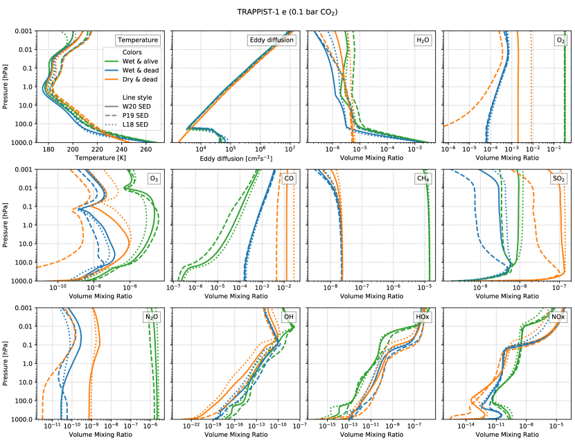
Figure 7: Temperature, eddy diffusion coefficients and composition profiles of TRAPPIST-1 e runs with 0.1 bar CO₂. Different colors represent the three scenarios considered: green for wet & alive, blue for wet & dead and orange for dry & dead. Solid lines represent results using the input TRAPPIST-1 W20 SED, dashed lines show profiles using the P19 SED and dotted lines represent the output using the L18 SED (see also Figure 6).

4.1.1 Temperature

Table 12: $T_{\text{surf}}$ in K of TRAPPIST-1 e for all three scenarios with 0.1 bar CO₂ and different input SED of TRAPPIST-1.

Input SED	Wet & alive	Wet & dead	Dry & dead
W20 SED	273.1	269.6	251.5
P19 SED	272.2	268.2	250.4
L18 SED	273.7	270.9	252.7

Figure 7 shows temperature, eddy diffusion coefficient and composition profiles for selected species for TRAPPIST-1 e with 0.1 bar CO₂. The different scenarios are distinguished by color and the different stellar input spectra are denoted by different line styles. The temperature profiles are very similar for all runs except near the surface where the greenhouse effect of H₂O leads to larger temperatures for the wet scenarios compared to the dry & dead runs. The temperature inversion in the middle atmosphere is lacking due to weak UV absorption by O₃ (see Section 4.1.6). The wet & alive runs show the largest $T_{\text{surf}}$ due to warming from biogenic species such as CH₄ (see Table 12). The impact of the different stellar spectra shown in Figure 6 on the planetary $T_{\text{surf}}$ is generally small.

4.1.2 Eddy diffusion coefficients

For the dry scenario the eddy diffusion coefficient, $K$, near the surface is low and increases continuously towards higher altitudes. This is similar to the $K$ profiles estimated for Venus and Mars (e.g. Nair et al., 1994; Krasnopolsky, 2012). The wet scenarios follow a $K$ profile which is similar to Earth with a decrease of $K$ up to the cold trap and an increase above (Massie & Hunten, 1981). This profile is also similar to that calculated by Lincowski et al. (2018) for the atmosphere of TRAPPIST-1 e, assuming an Earth-like planet covered by an ocean.

4.1.3 H₂O

The water profile in the lower atmosphere depends mainly on the fixed relative humidity and the temperature. For the wet scenarios the relative humidity profile is assumed to be constant at 80% in the lower atmosphere. For the dry runs only the surface H₂O is calculated with the relative humidity, otherwise the H₂O profile is determined chemically. For pressures below 1 hPa H₂O is mainly destroyed photochemically at wavelengths shorter than 200 nm and reformed via HO_x-driven (HO_x = H + OH + HO₂) oxidation of CH₄ into H₂O. The scenario which includes biogenic fluxes of the Earth as additional lower boundary condition (wet & alive) leads to significant H₂O production via CH₄ oxidation (see also Segura et al., 2005; Grenfell et al., 2013; Rugheimer et al., 2015; Wunderlich et al., 2019).

4.1.4 CH₄

The abundances of CH₄ are mainly driven by the surface flux. For the alive scenario we use pre-industrial (biogenic and volcanic) flux measured on Earth (6.31$\cdot$10¹⁰ cm s^-1, see Table 4) and for the dead runs we use only geological sources of CH₄ (1.12$\cdot$10⁸ cm s^-1, see Table 4). The choice of the SED has no impact on the CH₄ abundances in the lower atmosphere. For pressures below 0.1 hPa, where destruction of CH₄ is dominated by photolysis, the choice of the SED has only a weak impact on the CH₄ concentrations. As found in previous works the CH₄ abundances are increased for a planet orbiting an M-dwarf compared to a few ppm on Earth (e.g. Segura et al., 2005; Grenfell et al., 2013, 2014; Rugheimer et al., 2015; Wunderlich et al., 2019). This is mainly due to reduced sources of OH via e.g. H₂O + O(¹D)  $\rightarrow$ 2 OH, where O(¹D) comes mainly from O₃ photolysis in the UV. Cool stars, such as TRAPPIST-1 are weak UV emitters, favoring a slowing in the OH source reaction and less destruction of CH₄ by OH (see e.g. Grenfell et al., 2013).

In Wunderlich et al. (2019) we modelled an Earth-like planet with Earth’s biofluxes around TRAPPIST-1 and found that the atmosphere would accumulate about 3000 ppm of CH₄. The much lower value of around 15 ppm suggested by this study is due to two main reasons. First, for this study we only consider the natural sources of CH₄, whereas in Wunderlich et al. (2019) we also included anthropogenic sources. CH₄ emissions similar to modern Earth would correspond to a very short period of Earth’s history whereas pre-industrial emissions of CH₄ persisted for a much longer time. Second, we consider a non-zero CH₄ deposition velocity of 1.55$\cdot$10^-4 cm/s, reducing the amount of CH₄ accumulated in the atmosphere. We use this measured deposition velocity of CH₄ to validate our model against Earth (see Section 2.4.1). With a zero deposition we would overestimate modern Earth amounts of CH₄ and hence, we also consider a deposition of CH₄ for the TRAPPIST-1 planets.

4.1.5 O₂

The alive scenario assumes a constant Earth-like O₂ flux from photosynthesis rather than a constant mixing ratio at the surface. The resulting mixing ratio for TRAPPIST-1 e with 0.1 bar CO₂ is around 35 %. The increase of O₂ compared to Earth is consistent with results of Gebauer et al. (2018a), who found that the required flux to reach a certain O₂ concentration is reduced on an Earth-like planet around AD Leo compared to the Earth around the Sun. This is due to the lower UV flux of M-dwarfs, compared to solar like stars, resulting in weaker destruction of O₂ in an Earth-like planetary atmosphere. However, for an atmosphere with about 0.35 bar O₂ forest ecosystems would be unlikely because the frequency of wildfires is expected to be increased, preventing the build-up of larger concentrations of O₂ (see e.g. Watson, 1992; Kump, 2008). This effect is not considered in the model.

For the dry & dead runs there is a large spread of O₂ abundances ranging from surface concentrations below 1 ppm using the P19 SED to almost 1 % using the L18 SED. This spectrum has the largest stellar FUV/NUV ratio, which was shown to favor the abiotic build-up of O₂ in CO₂-rich atmospheres as follows (see e.g. Selsis et al., 2002; Segura et al., 2007; Tian et al., 2014; France et al., 2016): CO₂ photolysis below 200 nm leads to CO and atomic oxygen. Then either atomic oxygen produces O₂ (by e.g. O + O + M $\rightarrow$ O₂ + M or O + OH + M$\rightarrow$ O₂+ H + M) or is recombined with CO via the HO_x catalysed reaction sequence, which results overall in CO₂ forming: CO + O $\xrightarrow[]{\text{HO${}_{x}$}}$ CO₂ (see e.g. Selsis et al., 2002; Domagal-Goldman et al., 2014; Gao et al., 2015; Meadows, 2017). The reduced production of HO_x by H₂O destruction in the lower atmosphere for the dry & dead cases, compared to the wet & dead runs, leads to more favorable conditions for abiotic O₂ build-up. Additionally the deposition of O₂ into an unsaturated ocean, as assumed for the wet & dead cases, is stronger than the deposition onto desiccated surfaces for the dry cases (see Kharecha et al., 2005; Domagal-Goldman et al., 2014).

4.1.6 O₃

The production of O₃ in the middle atmosphere depends on the O₂ concentration and the UV radiation in the Schumann-Runge bands and Herzberg continuum (from about 170 nm to 240 nm). The destruction of O₃ is mainly driven by absorption in the Hartley (200 nm - 310 nm), Huggins (310 nm - 400 nm), and Chappuis (400 nm - 850 nm) bands. HO_x and NO_x destroy O₃ via catalytic loss cycles in the middle atmosphere (see e.g. Brasseur & Solomon, 2006; Grenfell et al., 2013). For the scenario with constant O₂ flux of 1.21$\cdot$10¹² molecules cm^-2 s^-1, more O₃ is produced than for the dead runs, where O₂ is only produced abiotically. For the L18 SED with lower UV flux between 170 and 240 nm, the O₃ layer is weaker than for the runs using the other stellar spectra. Due to enhanced abundances of O₂ compared to Earth, we find that more O₃ is produced. O’Malley-James & Kaltenegger (2017) suggested a weaker O₃ layer as on Earth, assuming an O₂ surface partial pressure of 0.21 bar.

4.1.7 CO

Photolysis of CO₂ in the UV produces CO and O. The dry scenario builds up more CO than the wet cases. For the alive runs with additional O₂ surface sources, the CO recombines more efficiently to CO₂ (via CO + O $\xrightarrow[]{\text{HO${}_{x}$}}$ CO₂), resulting in lower CO amounts compared to the dead runs. Additionally we assume a net deposition of CO from the atmosphere to the soil-vegetation system, reducing the amount of CO accumulated in the atmosphere (e.g. Prather et al., 1995; Sanhueza et al., 1998). As for O₂, the abundances of CO are larger for the dry & dead runs than the wet & dead runs mainly due to the assumed strong uptake of CO by the ocean for the wet scenario.

The CO mixing ratios are comparable to the results of Hu et al. (2020). For an atmosphere consisting of 1 bar N₂ and 0.1 bar CO₂ they suggest a partial pressure of CO of about 0.05 bar using a weak $\nu_{\text{dep}}$ of 1$\cdot$10^-8 cm/s and a CO partial pressure of $\sim$1$\cdot 10^{-4}$ bar assuming a direct recombination reaction of O₂ and CO in the ocean. The less effective build-up of CO and abiotic O₂ due to a strong surface sink gives indirect evidence on the presence of a liquid ocean. Hence, under the simulated conditions with strong CO₂ photolysis, CO could not only serve as an ”antibiosignature” gas as discussed in e.g. Zahnle et al. (2008); Wang et al. (2016); Nava-Sedeño et al. (2016); Meadows (2017); Catling et al. (2018) and Schwieterman et al. (2019) but would indirectly suggest the absence of a liquid ocean at the surface.

The largest abundances of CO for the dry scenarios are found using the L18 SED. This is due to the lower abundances of HO_x, in particular OH, which reduce the recombination of CO + O into CO₂. In turn, large amounts of HO_x, like for the dry scenario using the P19 SED, lead to low build-up of CO.

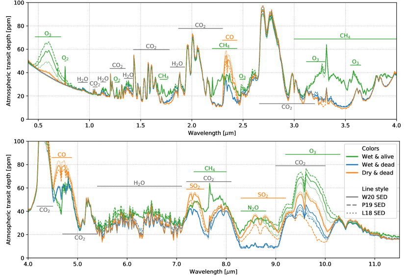
Figure 8: Simulated atmospheric features of the TRAPPIST-1 e runs with 0.1 bar CO₂, represented by cloud-free transit transmission spectra and binned to a constant resolving power of $R$=300 (maximum resolving power of NIRSpec PRISM at 5 $\mu$m). Important atmospheric molecular absorption bands are highlighted with horizontal lines in the color of the scenario with the strongest feature or in gray when all scenarios show a strong feature.

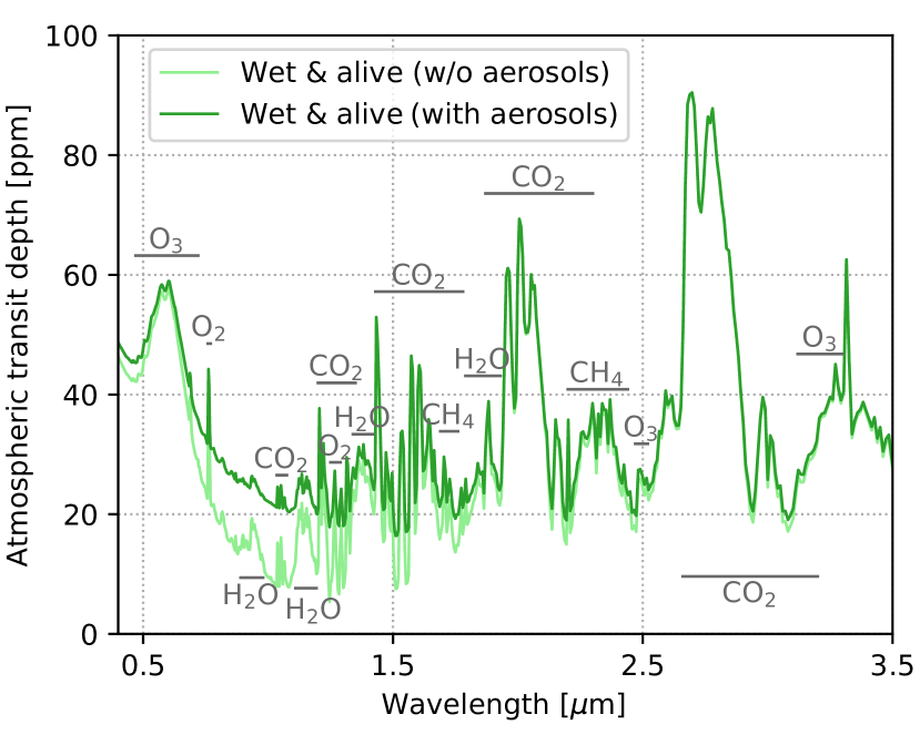
Figure 9: Simulated transmission spectrum of the TRAPPIST-1 e wet & alive run with 0.1 bar CO₂ with and without the impact of aerosol extinction.

4.1.8 SO₂

The main source of SO₂ is volcanic outgassing, which is assumed to be equally distributed over the first 10 km of the atmosphere. For a 1 bar N₂ atmosphere with 0.1 bar CO₂, this corresponds to pressure levels below $\sim$250 hPa. The large $\nu_{\text{dep}}$ of 1 cm/s (Sehmel, 1980) leads to a strong decrease of SO₂ towards the surface for all three scenarios. Due to its large solubility in water, SO₂ is deposited easily over wet surfaces, such as oceans. However, Nowlan et al. (2014) showed that over desert areas the $\nu_{\text{dep}}$ of SO₂ is approximately 0.5 cm/s, hence our value of 1 cm/s which is applied for dry cases as well may overestimate the deposition.

For the wet scenarios we assume Earth-like wet deposition following Giorgi & Chameides (1985). Most SO₂ dissolves into condensed water and is rained out of the atmosphere as sulfate. This process greatly decreases the mixing ratio of SO₂ for the wet cases but not for the dry scenarios.

The remaining SO₂ is transported upwards and is partly destroyed by photolysis. SO₂ photodissociates below 400 nm and strongest below 250 nm (e.g. Manatt & Lane, 1993). Hence, for the scenarios using the P19 SED we find the strongest destruction of SO₂ above 100 hPa.

4.1.9 N₂O

The main N₂O source on Earth are surface biomass emissions. For the alive scenario we find concentrations of N₂O comparable to previous studies such as Rugheimer et al. (2015) and Wunderlich et al. (2019). The photodissociation of N₂O is closely related to the SED around 180 nm (e.g. Selwyn et al., 1977), leading to lower abundances of N₂O using the P19 SED.

4.2 Transmission spectra of TRAPPIST-1 e with 0.1 bar CO₂

Figure 8 shows the simulated transmission spectra of the TRAPPIST-1 e atmosphere scenarios with surface partial pressures of 0.1 bar CO₂, binned to a constant resolving power of $R$=300. The spectra are simulated by the GARLIC model taking as input the chemical and temperature profiles discussed in Section 4.1. We do not take into account the effect of clouds but we include weak extinction from aerosols (see Fig. 9).

The CO₂ absorption features are similarly strong for all runs. The wet & alive runs show strong absorption of O₃ in the VIS at around 600 nm and in the IR at 9.6 $\mu$m. The alive run with the P19 SED shows the largest O₃ features, due to the more pronounced O₃ layer in the middle atmosphere compared to the runs using the other SEDs. The spectral features of abiotic production of O₃ and O₂ for the dead runs are generally much weaker than the biogenic features. This suggests that only the O₃ feature at 9.6 $\mu$m could lead to a false positive detection of O₃.

The CH₄ feature at 2.3 $\mu$m which is visible for the alive runs overlaps in low resolution with the CO feature which occurs for the dead & dry runs. The dead runs using the W20 and L18 SEDs show much larger absorption of CO at 2.3 $\mu$m than the wet & dry runs. For the dead runs with the P19 SED wet and dry conditions are not clearly distinguishable due to the weak build-up of CO in the dry run (see Section 4.1.7).

Weak H₂O absorption in the lower atmosphere of the dry runs result in more pronounced spectral windows between e.g. 1.7 and 1.8 $\mu$m. The H₂O features between 5.5 and 7 $\mu$m do not show a large difference for the various scenarios since these are dominated by absorption higher up in the atmosphere, where the H₂O concentration is predominantly determined by photochemical processes and similar for all cases.

4.3 Atmospheres with increasing CO₂

Table 13: $T_{\text{surf}}$ in K of TRAPPIST-1 e or TRAPPIST-1 f for all scenarios and increasing amount for CO₂. The W20 SED is used as input for the atmospheric model.

Planet	CO2 (bar)	Wet & alive	Wet & dead	Dry & dead
e	10-3	245.6	245.9	238.3
e	0.01	256.7	253.3	242.7
e	0.1	273.1	269.6	251.5
e	1	335.7	331.6	281.1
f	3.6	279.6	272.7	233.5
f	10.8	330.2	327.0	258.9

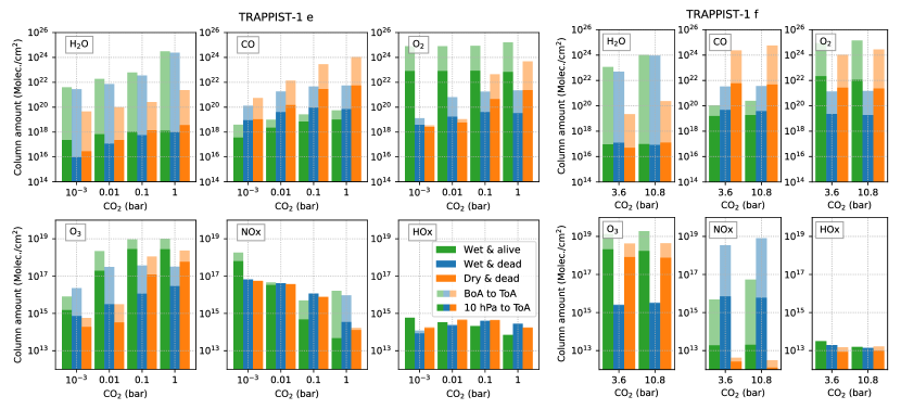
Figure 10: Column amounts (molecules cm^-2) of H₂O, CO, O₂, O₃, HO_x and NO_x for all atmospheric scenarios of TRAPPIST-1 e (left) and TRAPPIST-1 f (right) with increasing partial pressures of CO₂ (see also Table 11). Semi transparent bars show column amounts integrated from BoA to ToA and full filled bars show column amounts integrated from 10 hPa to ToA.

Figure 10 shows the column amount of H₂O, CO, O₂, O₃, NO_x and HO_x for all three scenarios and with increasing partial pressures of CO₂ for TRAPPIST-1 e (left) and TRAPPIST-1 f (right). Semi transparent bars represent column amounts integrated over the entire atmosphere whereas solid filled bars show upper column amounts integrated at pressures below 10 hPa, dominated by photochemical processes. For simulations shown in Figure 10 we use the W20 SED as input for the climate-chemistry model.

4.3.1 H₂O

The H₂O amount near the surface mainly depends on the relative humidity and the near surface temperature, leading to an increase of the H₂O amount towards larger CO₂ partial pressures. Whereas the dry runs show a lower H₂O content integrated over the entire atmosphere than the wet runs, at pressures below 10 hPa the three scenarios are comparable (see also Fig. 6). The $T_{\text{surf}}$ for TRAPPIST-1 e with 1 bar CO₂ and TRAPPIST-1 f with 10.8 bar CO₂ is $\sim$ 340 K for the wet runs. While the total H₂O amount increases for an increasing $T_{\text{surf}}$, the increase in the upper atmospheric column is much less, which suggests that tropospheric climate is difficult to elucidate from observing middle atmosphere H₂O. Further, the mixing ratio below 10^-5 (see Fig. 7) suggests that H₂O loss due to H₂O photolysis and hydrogen escape is expected to be weak for CO₂-rich atmospheres according to Wordsworth & Pierrehumbert (2013).

4.3.2 CO

As discussed in Section 4.1 dry & dead conditions favor an increase in atmospheric CO compared to the wet runs. With increasing CO₂ this effect is strengthened due to the enhanced CO₂ photolysis for intermediate CO₂ amounts. For CO₂ partial pressures of 1 bar there is only weak increase of CO column amounts compared to the atmosphere with 0.1 bar CO₂, if the $\nu_{\text{dep}}$ of CO is 1$\cdot$10^-8 cm/s. For TRAPPIST-1 f runs with 90% CO₂ there is only weak increase of CO compared to the TRAPPIST-1 e run with 50% CO₂ (1 bar partial pressure of CO₂). This is consistent with results of Hu et al. (2020). They suggest, that in CO₂-rich atmospheres of TRAPPIST-1 e a nonzero deposition velocity of 1$\cdot 10^{-8}$cm s^-1 leads to a maximum build-up of CO of around 0.05 bar.

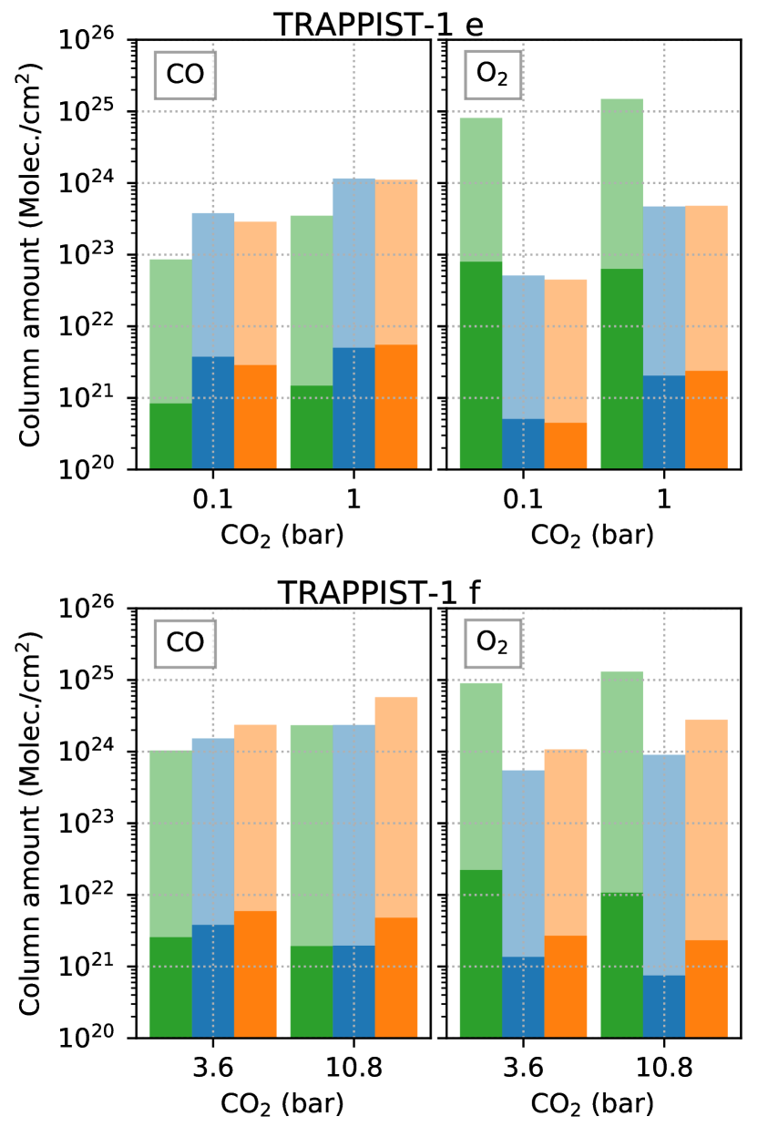
Figure 11: Same as Figure 10 but with a $\nu_{\text{dep}}$ = 1$\cdot$10^-8 cm/s for O₂ and CO, assuming that the wet runs have an ocean saturated with these gases and the biosphere is not an effective sink for CO. Only O₂ and CO are shown because the other species show similar abundances to Figure 10.

For the wet scenarios we assume a much faster deposition of CO due to uptake of the ocean and/or vegetation. The fact that the amount of HO_x is approximately the same for dry and wet surface conditions (see Fig. 10), suggests that for wet atmospheres with low CO₂ the fast deposition of CO accounts for the weak accumulation of CO.

We also simulated the abundances of CO and O₂ for the wet scenarios assuming that the deposition of CO and O₂ into an ocean is weak (see Fig. 11). We find that the concentrations of CO would be equally high for wet & dry conditions. Only for the CO₂-dominated atmosphere of TRAPPIST-1 f more CO would be present in the dry run compared to the wet runs.

Figure 12: O₃ and related composition profiles of TRAPPIST-1 e wet & alive runs with 10^-3 bar CO₂ (dotted line), 0.01 bar CO₂ (dashed line) and 0.1 bar CO₂ (solid line).

4.3.3 O₂

For the alive scenario the abundance of O₂ is mainly driven by the biogenic surface flux, which is equally strong in all alive runs. Due to the high FUV/NUV ratio for TRAPPIST-1 we expect that significant amounts of O₂ are produced abiotically from CO₂ photolysis. The potentially false positive detection of O₂ in CO₂ atmospheres was already discussed by several studies (e.g. Selsis et al., 2002; Segura et al., 2007; Harman et al., 2015; Meadows, 2017). Figure 7 shows that the abundances of abiotic O₂ increase for dry CO₂-dominated atmospheres but are always lower than expected from a biosphere similar to the Earth. On the other hand for wet conditions without a biosphere much less abiotic O₂ is accumulated in a CO₂-dominated atmosphere. This means that weak biogenic O₂ flux would not be distinguishable from a dry N₂ atmosphere with at least 0.1 bar CO₂.

4.3.4 O₃, NO_x and HO_x

The three scenarios show a different O₃ behaviour with increasing CO₂ (see Fig. 10). The alive run with the lowest amount of CO₂ accumulates large amounts of NO_x, destroying most of the O₃. With increasing abundances of CO₂, the temperature increases (see Table 13) and more H₂O evaporates. This leads to more HO_x near the surface, more removal of NO_x into reservoirs such as HO₂NO₂ and less catalytic destruction of O₃ by NO_x (see Fig. 12).

For the dead runs the O₃ is produced abiotically and increases for atmospheres with more CO₂. The dry & dead runs have rather low concentrations of NO_x and HO_x for CO₂-dominated atmospheres, which suggests a weak gas-phase effect upon O₃ for these species. In contrast, the wet & dead conditions lead to a build-up of NO_x for TRAPPIST-1 f with 90% CO₂ near the surface, resulting in very low O₃ abundances in the lower atmosphere.

4.4 Transmission spectra for increasing CO₂

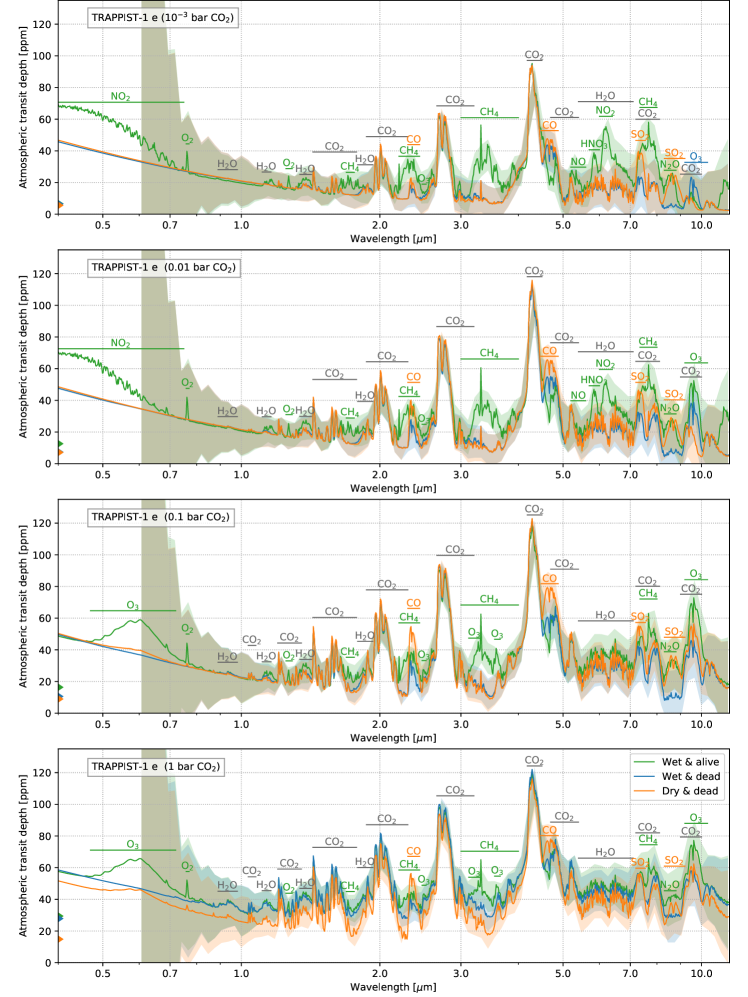
Figure 13: Simulated atmospheric features of TRAPPIST-1 e runs, represented by cloud-free transit transmission spectra and binned to a constant resolving power of $R$=300 (maximum resolving power of NIRSpec PRISM at 5 $\mu$m). Individual plots from top to bottom show atmospheres with increasing partial pressures of CO₂. Shaded regions represent the one sigma error of 30 co-added transit observations with JWST NIRSpec PRISM and MIRI LRS, binned to $R$=30 (minimum resolving power of NIRSpec PRISM at 1 $\mu$m). Important atmospheric molecular absorption bands are highlighted with horizontal lines in the color of the scenario with the strongest feature or in gray when all scenarios show significant features. Coloured triangles indicate minimum atmospheric transit depth of each scenario.

Figure 13 shows the simulated atmospheric appearance of TRAPPIST-1 e during primary transit for the three scenarios and for increasing amounts of CO₂. Several molecular features distinguish the alive run with 10^-3 bar CO₂ from the dead runs. Features from CH₄, O₂ and N₂O are present due to the assumed biogenic flux. Strong CH₄ features are especially prevalent in Earth-like atmospheres with low UV environments in the habitable zone around M-dwarfs (e.g. Segura et al., 2005; Rauer et al., 2011; Wunderlich et al., 2019). Additionally we find a strong NO₂ feature in the VIS as well as NO₂, NO and HNO₃ features between 5 and 7 $\mu$m due to the large amounts of these species in cold, CO₂-poor alive runs (see Fig. 12). These features are found to be present also for strong flaring conditions with cosmic-ray-induced amounts of NO₂ (see e.g. Tabataba-Vakili et al., 2016; Scheucher et al., 2018, 2020). The typical O₃ band around 9.6 $\mu$m is absent due to the large abundances of NO_x species, which can destroy O₃ catalytically.

The dead runs with low CO₂ abundances show little spectral differences between wet and dry scenarios. Only SO₂ features around 7.5 and 8.5 $\mu$m and weak CO bands around 2.3 $\mu$m and 4.7 $\mu$m distinguish the dry & dead run from the wet & dead run. With increasing CO₂ the larger abundances of CO for dry & dead conditions lead to stronger CO absorption bands and clearly separate dry from wet runs. The presence of the CO bands for CO₂-rich atmospheres was also shown by e.g. Meadows (2017) and Schwieterman et al. (2019).

For CO₂ partial pressures of 0.1 bar and above, NO_x is reduced and its spectral features do not appear in the transmission spectrum. O₃ abundances are increased and molecular bands show up in the VIS and at 9.6 $\mu$m. The CH₄ abundances are very similar for all runs and hence the CH₄ absorption at 2.3 $\mu$m and 3.3 $\mu$m for a 1 bar CO₂ should be as strong as for a CO₂-poor atmosphere. However, the increase in CO₂ abundances lead to larger lower atmosphere temperatures, hence more H₂O in this region. Since H₂O absorbs over a wide wavelength range this results in an increase in the offset of the entire spectrum (see e.g. Turbet et al., 2019), reducing the CH₄ features relative to the overall absorption. This is also suggested by Table 14, showing the baseline of TRAPPIST-1 e transmission spectra from Figure 13.

Table 14: Minimum atmospheric transit depth, $t_{\text{min}}$ (ppm) and corresponding $\lambda$ ($\mu$m) of the transmission spectra of TRAPPIST-1 e for all three scenarios and different amount of CO₂. $t_{\text{min}}$ is calculated for a constant $R$ of 300 in the NIRSpec PRISM wavelength range (0.6 - 5.3 $\mu$m).

	Wet & alive		Wet & dead		Dry & dead
CO2	$t_{\text{min}}$	$\lambda$	$t_{\text{min}}$	$\lambda$	$t_{\text{min}}$	$\lambda$
(bar)	(ppm)	($\mu$m)	(ppm)	($\mu$m)	(ppm)	($\mu$m)
10-3	9.44	3.06	6.51	3.51	6.39	3.51
0.01	12.63	2.14	7.39	3.51	7.11	3.51
0.1	16.37	1.51	10.59	3.51	8.96	3.51
1	29.44	1.25	27.86	2.24	14.84	2.24

Note. — $t_{\text{min}}$ depends on $R$ and the considered wavelength range.

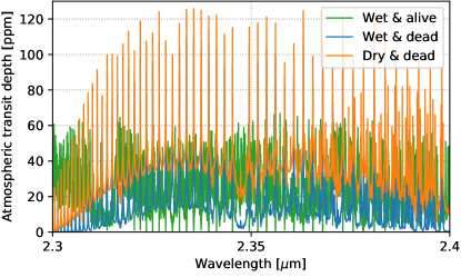
Figure 14: High resolution transmission spectra of TRAPPIST-1 e runs with 0.1 bar CO₂ with a resolving power of $R$=100,000, appropriate for the ELT HIRES. Green line: CH₄ features of the wet & alive run. Blue lines: CO features of the wet & dead run. Orange line: CO features of the dry & dead run. Absorption from species other than CO or CH₄ are subtracted from the spectrum.

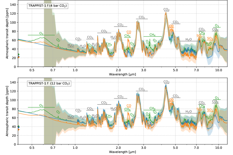
Figure 15: Same as Figure 13 but for TRAPPIST-1 f runs.

The most promising candidates for distinguishing the three scenarios from each other are the CH₄ features, which are just evident in the alive runs as well as strong CO bands for the dry runs. Absorption of CH₄ and CO features overlap at 2.3 - 2.5 $\mu$m, which could inhibit their separation. A simultaneous observation of CH₄ at 3.3 $\mu$m is therefore required as well as measurements of CO at 4.6 $\mu$m. Using JWST NIRSpec PRISM covers 0.60 - 5.30 $\mu$m, however TRAPPIST-1 is close to the saturation limit of NIRSpec PRISM (J $<$ 10.5), resulting in a low duty cycle (see e.g. Batalha & Line, 2017). We do not consider a partial saturation strategy to improve the duty cycle as suggested by Batalha et al. (2018). NIRSpec G235M only covers 1.66 - 3.12 $\mu$m, hence would not be suitable for separating CH₄ and CO. Another possibility to disentangle both features is by observing individual lines with high resolution spectroscopy (HRS). Figure 14 shows the simulated transmission spectra of the TRAPPIST-1 e runs with 0.1 bar CO₂, binned to the resolution of ELT HIRES ($R$=100,000). Since the position of the lines relative to each other differ between CO and CH₄ one could use the cross-correlation technique to determine which absorber causes the spectral lines or even if both species are present.

The transmission spectra of the TRAPPIST-1 f atmospheres show similar spectral features to those of TRAPPIST-1 e with 1 bar CO₂ (see Figure 15).

4.5 Detectability of spectral features

Table 15: Number of transits required to detect spectral features with an S/N of 5 in a cloud-free TRAPPIST-1 e atmosphere with 0.1 bar CO₂ using LRS with JWST NIRSpec or JWST MIRI and HRS with ELT HIRES. For LRS, $\lambda$ corresponds to the central wavelength of the spectral feature whereas for HRS the considered wavelength range is given. For JWST NIRSpec the filter with the largest S/N for the spectral feature is considered (see Table 8 and Figure 5). For potentially detectable features the required number of transits using JWST NIRSpec PRISM is given in parenthesis. Numbers below 30 are highlighted in bold face.

Telescope	Specie ($\lambda$)	Wet & alive	Wet & dead	Dry & dead
JWST	CO2 (4.3 $\mu$m)	5 (11)	4 (9)	4 (8)
ELT	CO2 (1.8-2.3 $\mu$m)	33	28	26
JWST	H2O (1.4 $\mu$m)	170	107	100
ELT	H2O (1.3-2.0 $\mu$m)	1224	1424	865
JWST	CH4 (3.3 $\mu$m)	60 (60)	-	-
ELT	CH4 (2.1-2.5 $\mu$m)	26	7,434	$>$10,000
JWST	CO (2.35 $\mu$m)	-	114	19 (57)
ELT	CO (2.3-2.45 $\mu$m)	437	105	42
JWST	O3 (9.6 $\mu$m)	124	255	258
ELT	O3 (3.4-3.7 $\mu$m)	4,024	$>$10,000	$>$10,000
JWST	O2 (1.27 $\mu$m)	3,012	-	-
ELT	O2 (1.24-1.3 $\mu$m)	910	$>$10,000	$>$10,000
JWST	SO2 (7.35 $\mu$m)	-	-	146
ELT	SO2 (3.9-4.1 $\mu$m)	-	-	$>$10,000
JWST	N2O (8.5 $\mu$m)	1,292	-	-
ELT	N2O (2.1-2.3 $\mu$m)	951	-	-

Note. — The ETC for the ELT does not include the wavelength range 2.9-3.4 $\mu$m which will be covered by METIS (Brandl et al., 2016). Since O₃ absorbs in the L-band we might overestimate the number of transits required to detect O₃.

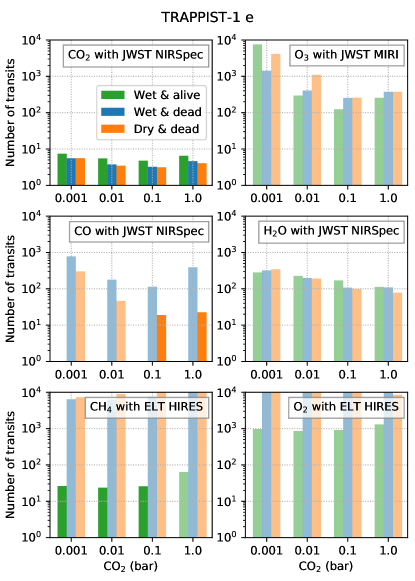
Figure 16: Number of transits required to reach an S/N of 5 for the corresponding spectral features of CO₂ at 4.3 $\mu$m, O₃ at 9.6 $\mu$m, CO at 2.35 $\mu$m and H₂O at 1.4 $\mu$m with JWST NIRSpec (upper and middle panel) and CH₄ from 2.1 to 2.5 $\mu$m and O₂ from 1.24 to 1.3 $\mu$m with ELT HIRES (lower panel) in a cloud-free atmosphere of TRAPPIST-1 e. The x-axes correspond to the increasing partial pressures of CO₂. Full filled bars: required number of transits is below or equal 30. Semi transparent bars: required number of transits is larger than 30.

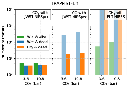
Figure 17: Number of transits required to reach an S/N of 5 for the corresponding spectral features of CO₂ at 4.3 $\mu$m and CO at 2.35 $\mu$m with JWST NIRSpec (left and center) and CH₄ from 2.1 to 2.5 $\mu$m with ELT HIRES (right) in a cloud-free atmosphere of TRAPPIST-1 f. The x-axes correspond to the increasing partial pressures of CO₂. Full filled bars: required number of transits is below or equal 30. Semi transparent bars: required number of transits is larger than 30.

We determine the required number of transits necessary to detect a spectral feature (S/N = 5) with JWST NIRSpec or JWST MIRI. We bin the spectral data until the optimal value is found, leading to the lowest required number of transits. Binning the data decreases the noise contamination but if the binned wavelength range is too large, molecular absorption bands and atmospheric windows overlap, leading to a cancellation of the spectral feature. Due to the unknown systematic error when binning the synthetic spectral data we assume only white noise. This gives an optimistic estimation on the detection feasibility of the JWST. Additionally we estimate the number of transits required to detect spectral absorption lines with ELT HIRES using the cross correlation technique without binning the spectral data (see Section 2.6).

4.5.1 CO₂

Table 15 shows the number of transits needed to detect selected spectral features for all three atmospheric scenarios of TRAPPIST-1 e with 0.1 bar CO₂. For all the calculations we assume cloud-free atmospheric conditions with weak extinction from aerosols (see Eq. (3)).

With JWST NIRSpec G395M/F290LP only about 5 transits are needed to detect the 4.3 $\mu$m CO₂ feature in a cloud-free atmosphere. About twice as many transits are required to detect CO₂ with NIRSpec PRISM. This result is in agreement with other studies such as Fauchez et al. (2019), who showed that the CO₂ at 4.3 $\mu$m of a 1 bar CO₂ atmosphere of TRAPPIST-1 e would be detectable with JWST NIRSpec PRISM by co-adding 9 transits without the existence of clouds. When taking clouds into account, they suggested that 19 transits are required to detect CO₂. For a ground-based telescope such as ELT at wavelengths longer than 4 $\mu$m, the noise contribution from the Earth’s atmosphere leads to very low S/N. The 2.7 $\mu$m feature of CO₂ is not observable with ELT. Hence, only the CO₂ feature around 2.0 $\mu$m might be detectable with ELT HIRES in $\sim$30 transits.

The molecular bands for CO₂ do not greatly increase when increasing the abundances of CO₂ from 10^-3 bar to 1 bar, hence also the number of transits needed to reach the same S/N of 5 are similar for all runs (see Fig. 16). It was shown by Barstow et al. (2016) that even the Earth and a 1 bar Venus-like atmosphere would show similar CO₂ features, which complicates the determination of the underlying atmospheric main composition by retrieval methods.
 

4.5.2 H₂O

A larger CO₂ partial pressure warms the lower atmosphere, leading to more H₂O evaporation in the case of a liquid reservoir. This leads to a more opaque lower atmosphere and an increase in the measured planetary radius (see e.g. von Paris et al., 2011; Madhusudhan & Redfield, 2015). In contrast, in the photochemical regime, H₂O is not greatly increased for warmer surface conditions (see Fig. 10). The effect of the radius increase is much weaker for dry atmospheres, leading to a better detectability of H₂O for dry surface conditions. However, the H₂O spectral features are too weak in all simulated atmospheres of TRAPPIST-1 e and TRAPPIST-1 f to allow for a detection with JWST NIRSpec. This was also concluded by Fauchez et al. (2019) who found that about 150 transits are required to detect H₂O in a cloud-free 1 bar CO₂ atmosphere of TRAPPIST-1 e with JWST.

Most H₂O bands in the NIR overlap with CH₄ absorption features. This could cause a false positive detection of H₂O for large abundances of CH₄ (see e.g. Wunderlich et al., 2019). The cross-correlation technique could disentangle H₂O from CH₄ but we find that by using the largest $\sim$500 H₂O lines about $\sim$1000 transits would be needed to detect H₂O with ELT HIRES.

4.5.3 CH₄

In low CO₂ atmospheres with biogenic surface fluxes the number of CH₄ lines which we identify is much larger than the H₂O lines, enabling a detection of CH₄ with less than 30 transits using ELT HIRES. The detection of the simulated levels of CH₄ would be challenging with JWST NIRSpec.

In contrast to the alive runs, no CH₄ feature is detectable for the dead runs with only geological sources of CH₄. However, since the ability to detect CH₄ mainly depends on the assumed surface flux, which could be weaker for a potential biosphere on an M-dwarf planet (e.g. Cui et al., 2017) or stronger for enhanced volcanic outgassing of CH₄, the detection or non-detection of CH₄ alone would not confirm or rule-out the existence of a biosphere (see also Krissansen-Totton et al., 2018b).

4.5.4 CO

About 10% of CO₂ are needed to produce enough CO photochemically to enable a detection of its molecular absorption feature at 2.35 $\mu$m in a cloud-free atmosphere with JWST NIRSpec G235M if surface sinks of CO are inefficient. For the wet scenarios, with significant CO uptake by an ocean or a biosphere, results suggest, that CO would not be detectable, even for a CO₂-dominated atmosphere. The CO feature at 4.6 $\mu$m overlaps with the CO₂ absorption, requiring a retrieval analysis to disentangle both signals. Only about 10 transits are needed to detect the 4.6 $\mu$m band with JWST. The G395M filter of JWST would be favorable because the CO₂ band at 4.3 $\mu$m and the CO feature at 4.6 $\mu$m could be observed simultaneous.
The CO feature at 2.3 $\mu$m does not overlap with other strong absorption features in the transmission spectrum of the dry scenarios. However, 19 transits are required to detect the CO feature at 2.3 $\mu$m (see Table 15), twice as many as for the detection of the 4.6 $\mu$m CO feature.
The detection of CO with the cross correlation technique has been shown to be feasible for gas giants exoplanets (see e.g. de Kok et al., 2013; Brogi et al., 2014). We find that the detection of CO would require about 40 transits with ELT HIRES in a dry, CO₂-rich, cloud-free atmosphere of TRAPPIST-1 e and f.

4.5.5 Other molecules

Results suggest, that no other molecular absorption features would be observable with JWST or ELT for the atmospheres considered here. Even a detection of the strong NO₂ feature around 6.2 $\mu$m in an alive CO₂-poor atmosphere (see green line in top panel of Fig. 13) would require around 50 transits with JWST MIRI (not shown). The O₃, SO₂ and N₂O features lie in a spectral region where the stellar flux is too low to allow high S/N. The O₂ feature is not strong enough for a detection with JWST NIRSpec. As also suggested by Rodler & López-Morales (2014) we find that the 1.27 $\mu$m band is more favorable than the 0.76 $\mu$m band for detecting O₂ in a planetary atmosphere around a very late M-dwarf. We find that with ELT over 900 transits are required to detect O₂ by cross-correlating the lines between 1.24 and 1.3 $\mu$m, assuming an average throughput of 10% for ELT HIRES. This is consistent with the results of Rodler & López-Morales (2014), who suggested that hundreds of transits are needed to detect O₂ in the atmosphere of Earth around an M7 star at a distance similar to TRAPPIST-1 with ELT using a high resolution spectrograph with a throughput of $\sim$20% (see Origlia et al., 2010).

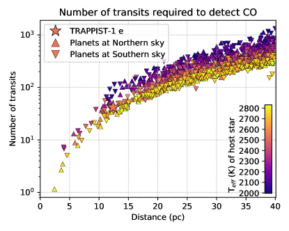
Figure 18: Number of transits required to detect CO with the cross correlation technique between 2.3 - 2.45 $\mu$m with ELT (Southern sky) or TMT (Northern sky) in the atmosphere of hypothetical planets with the same properties as TRAPPIST-1 e but around SPECULOOS targets. We assume that the atmosphere of all planets is that of the 0.1 CO₂ run with dry & dead conditions. The considered planetary atmospheric spectrum assumes cloud-free conditions.

4.5.6 SPECULOOS targets

With a distance of only 12.4 pc from the Sun, TRAPPIST-1 is one of the closest late-type M-dwarfs. However, we show that for the simulated atmospheres, only CO₂ would be potentially detectable within $\sim$10 transits. To further characterize the atmosphere of the planets observing the K-band with HRS might allow to determine whether a spectral feature around 2.3 $\mu$m can be attributed to absorption from CH₄ or CO. Our results suggest, that for a dry & dead atmosphere of TRAPPIST-1 e about 40 transits are required to detect CO with ELT HIRES. To detect an Earth-like O₂ feature with the same number of transits, a host star similar to TRAPPIST-1 is required at $\sim$7 pc or less (see Rodler & López-Morales, 2014; Serindag & Snellen, 2019).

The Search for habitable Planets EClipsing ULtracOOl Stars (SPECULOOS; Delrez et al., 2018b) is a ground-based transit survey which is looking for Earth-sized exoplanets around the nearest late M-dwarfs to brown dwarfs. Figure 18 shows the number of transits required to detect CO with the cross-correlation technique using TMT (Northern Sky) or ELT (Southern sky), assuming a hypothetical planet with the same properties as TRAPPIST-1 e around each member of the target list of SPECULOOS with a $T_{\text{eff}}$ of at least 2000 K (see Gillon et al., 2020). The assumed atmospheric spectral feature is the same as in the dry scenario with 0.1 bar CO₂.

There are only 13 stars within a distance of 7 pc ($T_{\text{eff}}>$2000 K), where the atmospheric O₂ feature of a hypothetical terrestrial planet would be detectable within 40 transits according to Rodler & López-Morales (2014). However, non-LTE effects in the O₂ 1.27 $\mu$m band may prevent a detection (López-Puertas et al., 2018). Figure 18 suggests that more targets exists for which the CO feature could be detected. For late M-dwarfs (2400 K$~{}<~{}T_{\text{eff}}~{}<$ 2800 K) CO could be detected up to $\sim$12pc using ELT or TMT by co-adding 30 transits. Early L-dwarfs ($T_{\text{eff}}<$2400 K) only have slightly smaller stellar radius than late M-dwarfs but are much fainter, resulting in a low S/N and more transits are required to detect atmospheric molecular features with transmission spectroscopy.

5 Discussion

With our climate-photochemistry model, 1D-TERRA, we simulated potential atmospheres of TRAPPIST-1 e and TRAPPIST-1 f. We determined the composition of the planetary atmospheres, assuming N₂ and CO₂-dominated atmospheres with wet and dry surface conditions. We did not consider O₂-rich atmospheres, accumulated from H₂O photolysis during the pre-main sequence phase of TRAPPIST-1 (see e.g. Wordsworth & Pierrehumbert, 2014; Luger & Barnes, 2015; Bolmont et al., 2016). However, an Earth-like biogenic flux of O₂ is considered and O₂ can also build up abiotically via CO₂ photolysis. For detailed discussion of the potential composition and transmission spectra of O₂-dominated atmospheres from H₂O photolysis we refer to Lincowski et al. (2018).

The main goal of our study was to investigate which spectral features of wet or dry planets in the habitable zone could be detectable with the upcoming JWST and ELT. We identify three species which could be detectable in a cloud-free atmosphere of TRAPPIST-1 e or f by co-adding less than 30 transits: CO₂, CH₄ and CO. Under the assumed boundary conditions, CO₂ would be detectable with JWST and ELT with about 10 transits. This is also consistent with several other studies investigating the detectability of the atmospheric features of the TRAPPIST-1 planets (Morley et al., 2017; Batalha et al., 2018; Krissansen-Totton et al., 2018a; Wunderlich et al., 2019; Lustig-Yaeger et al., 2019; Fauchez et al., 2019). However, for N₂-dominated atmospheres the uncertainties of the retrieved CO₂ abundances are up to 2 orders of magnitude when co-adding 10 transits (see Batalha et al., 2018; Krissansen-Totton et al., 2018a).

The effect of clouds and hazes is not considered in the model and we only consider weak extinction by aerosols for the simulation of the transmission spectra. We do not expect a large impact on the chemical composition when considering thin cloud or haze layers (see Venus validation, Figure 4). However, the presence of clouds can significantly reduce the detectability of molecular spectral features (see e.g. Kitzmann et al., 2011a, b; Vasquez et al., 2013; Benneke & Seager, 2013; Bétrémieux & Kaltenegger, 2014; Bétrémieux & Swain, 2017; Moran et al., 2018; Lustig-Yaeger et al., 2019; Fauchez et al., 2019; Komacek et al., 2020; Suissa et al., 2020). We use a similar expression to simulate the effect of aerosol absorption to Kaltenegger & Traub (2009). They conclude that the apparent radius of an atmosphere like on Earth is mainly determined by Rayleigh scattering and aerosol, H₂O and CO₂ absorption. For Earth, the inclusion of realistic cloud coverage has only a small effect on the apparent radius and hence, the detectability of spectral features.

For the wet scenarios with low CO₂ abundances and Earth-like biomass surface emissions we find that CH₄ would be detectable on TRAPPIST-1 e using the cross-correlation technique with less than 30 transits. Increasing the amount of CO₂ leads to additional greenhouse warming and more H₂O evaporated into the atmosphere. More H₂O in the lower atmosphere leads to an increase of the minimum transit depth in the transit spectrum, i.e. the observational baseline (see also Turbet et al., 2019). The strongest CH₄ feature at 3.3 $\mu$m is about 40 ppm above the baseline, when very little H₂O is present in the atmosphere. For a lower atmosphere with a relative humidity of 80% and a $T_{\text{surf}}$ of $\sim$335 K the baseline increases by 20 ppm compared to a cold atmosphere with a $T_{\text{surf}}$ of $\sim$245 K. Due to this effect, for CO₂-dominated atmospheres of TRAPPIST-1 e and TRAPPIST-1 f CH₄ would not be detectable for a pre-industrial Earth-like emission flux of CH₄, since this feature would be partially swamped by the baseline. For these cases the spectral appearance would not suggest the existence of a biosphere within the detection limits, i.e. it would be a false negative detection of CH₄.

Enhanced outgassing when assuming e.g. a more reducing mantle than modern Earth would need to be 2-3 orders of magnitudes larger than for modern Earth to build up as much CH₄ as for the alive scenarios (see also Ryan et al., 2006; Krissansen-Totton et al., 2018b). Since also the outgassing of CO is expected to be large for a highly reduced mantle, simultaneous detection of CO could distinguish an atmosphere with large amounts of outgassed abiotic CH₄ from an atmosphere with mainly biogenic CH₄ (see also Krissansen-Totton et al., 2018b).

The presence of large amounts of CO has been suggested to indicate the absence of life on an exoplanet (Zahnle et al., 2008; Wang et al., 2016; Nava-Sedeño et al., 2016; Meadows, 2017; Catling et al., 2018). We find that the CO feature at 2.3 $\mu$m would be detectable with JWST NIRSpec for a dry atmosphere with at least 0.1 bar CO₂ by co-adding $\sim$20 transits (Fig. 16). In contrast to CH₄, CO would be detectable also for CO₂-dominated atmospheres due to the enhanced CO build-up from CO₂ photolysis.

The detection of CO with ELT HIRES requires twice as much transits than with JWST when assuming an average throughput of 10%. Previous studies such as Snellen et al. (2013) or Serindag & Snellen (2019) assume a mean throughput of 20% for ELT. However, to achieve this large efficiency further development of the instrument design might be necessary (see e.g. Ben-Ami et al., 2018).

For dry surface conditions, without a liquid ocean, we expect that very little CO would be deposited onto the surface. In contrast, the existence of an ocean may inhibit the build-up of substantial amounts of CO in a CO₂-rich atmosphere through catalytic cycles and an effective CO surface sink. This would lead to a non-detection of CO for wet surface conditions. However, the detection of CO in a CO₂-rich atmosphere of an M-dwarf planet could be also compatible with the presence of an ocean and a biosphere with ineffective surface sinks of CO or increased CO surface flux (Krissansen-Totton et al., 2018b; Schwieterman et al., 2019). Hence, the detection of CO does not ultimately discriminate between wet and dry surface conditions but a non-detection of CO and a simultaneous detection of CO₂ in the atmosphere of a potential habitable TRAPPIST-1 planet can hint at an effective surface sink for CO, suggesting the existence of an ocean.

As for CO, we find that abundances of SO₂ are much larger for dry surface conditions than for wet conditions. For the wet scenarios, most of the SO₂ is oxidised into highly soluble sulfate hence efficiently removed from the atmosphere by wet and dry deposition. For the dry scenarios we do not consider any wet deposition. Loftus et al. (2019) suggests that the detection of an H₂SO₄-H₂O haze layer together with SO₂ indicate that the planet does not host significant surface liquid water. The large amounts of SO₂ we find for the dry surface conditions are consistent with their study. However, the detection of SO₂ would not be feasible for any of the dry runs of TRAPPIST-1 e and TRAPPIST-1f with JWST or ELT. Furthermore, the SO₂ may form a haze layer.

For the simulated N₂ and CO₂-dominated atmospheres, one would require large observational times to detect spectral features in the atmospheres of the TRAPPIST-1 planets with JWST or ELT (see also Morley et al., 2017; Batalha et al., 2018; Krissansen-Totton et al., 2018a; Wunderlich et al., 2019; Lustig-Yaeger et al., 2019; Gillon et al., 2020).

In this study we assume white noise only when co-adding multiple transits or binning spectral data to a lower resolution than observed. This assumption may underestimate the required number of transits significantly, especially for weak spectral features (see e.g. Fauchez et al., 2019). Imaging spectroscopy concepts such as the Large UV/Optical/Infrared Surveyor (LUVOIR, The LUVOIR Team, 2019) and the Habitable Exoplanet Observatory (HabEx, Mennesson et al., 2016) may provide new opportunities to observe the atmosphere of terrestrial planets (see e.g. Pidhorodetska et al., 2020). The angular separation between TRAPPIST-1 and TRAPPIST-1 e is only 2.4 milliarcseconds (mas), much smaller than for Proxima Centauri b (37 mas) (O’Malley-James & Kaltenegger, 2019). This might be too small to separate the star and the planets with LUVOIR or HabEx (see also Stark et al., 2015). Hence, transmission spectroscopy is the most promising way to constrain the atmospheric characteristics of the habitable TRAPPIST-1 planets in the next few decades.

The recent detection of H₂O absorption in the atmosphere of the habitable zone planet K2-18b is one example of how the existence of an H₂ envelope could enable the characterization of the atmosphere of potentially rocky planets (Benneke et al., 2019; Tsiaras et al., 2019). Initial observations of the TRAPPIST-1 planets showed no hint of cloud-free H₂ or helium dominated atmospheres, suggesting that atmospheres are dominated by heavier elements (de Wit et al., 2016, 2018; Wakeford et al., 2018; Burdanov et al., 2019). However, hydrogen-rich atmospheres with high-altitude clouds or hazes are also consistent with the observations of the TRAPPIST-1 planets (Moran et al., 2018). Such hydrogen-rich atmospheres of the planets would increase the scale height, leading to improved detectability of spectral features.

6 Summary and Conclusion

We introduced and validated our new chemical network, part of our updated 1D coupled climate-photochemistry model (1D-TERRA). The model is capable of simulating the atmosphere of terrestrial planets over a wide range of temperatures and pressures. Our chemical network is based on those presented by Hu et al. (2012) and Arney et al. (2016). Additionally we added chlorine chemistry and extended the sulphur chemistry with chemical reactions listed in Zhang et al. (2012), in order to simulate Venus-like atmospheres. We showed that the model is able to reproduce modern Earth as well as CO₂-dominated atmospheres such as present on modern Mars and Venus. The resulting composition profiles are consistent with observations and other photochemical models, dedicated to model the atmosphere of Mars (Nair et al., 1994; Krasnopolsky, 2010a) and Venus (Krasnopolsky, 2012; Zhang et al., 2012).

In this paper we simulated the potential atmospheres of the TRAPPIST-1 e and TRAPPIST-1 f planets assuming N₂ and CO₂-dominated atmospheres for three main scenarios regarding the lower boundary condition: first, a wet & alive atmosphere with an ocean as well as biogenic and volcanic fluxes as on Earth, second, a wet & dead atmosphere with an ocean and only volcanic outgassing and, third, a dry & dead atmosphere without an ocean and with only volcanic outgassing (see Table 11). We showed the simulated atmospheric composition and spectral appearance of TRAPPIST-1 e with 0.1 bar CO₂ using three different SEDs as input for the climate-chemistry model. To our knowledge ours is the first study which uses an SED of TRAPPIST-1 which was constructed based on measurements in the UV (Wilson et al., submitted).

Starting from an N₂-dominated atmosphere we increased the surface partial pressures of CO₂ from 10^-3 bar for TRAPPIST-1 e up to 10.8 bar for TRAPPIST-1 f. The main results regarding the composition of the simulated atmospheres are listed below.

Table 16: Important molecular absorption features and corresponding wavelength in $\mu$m of the simulated transmission spectra of TRAPPIST-1 e for all three scenarios and with CO₂-poor (10^-3, 0.01 bar) and CO₂-rich (0.1, 1 bar) atmospheres. In black: strong spectral features, in gray: weak spectral features.

Scenario	CO2-poor (10-3, 0.01 bar)	CO2-rich (0.1, 1 bar)
	O2 (0.76, 1.27)	O2 (0.76, 1.27)
	O3 (9.6)	O3 (0.6, 9.6)
Wet	CH4 (2.3, 3.3, 7.7)	CH4 (2.3, 3.3, 7.7)
& alive	NO2 (below 0.7, 3.45, 6.2)	-
	NO (5.3)	-
	HNO3 (5.85)	-
	N2O (8.5)	-
Wet	O3 (9.6)	O3 (9.6)
& dead	CO (2.35, 4.6)	CO (2.35)
	-	O2 (0.76, 1.27)
Dry	-	O3 (0.6, 9.6)
& dead	CO (2.35, 4.6)	CO (2.35, 4.6)
	SO2 (7.35, 8.7)	SO2 (7.35, 8.7)

• The alive runs with Earth-like biogenic flux accumulate about 50% more O₂ as on modern Earth due to Earth’s weaker UV environment and hence weaker O₂ sinks.

• For dry CO₂-rich atmospheres, the abiotic production of O₂ and O₃ is significant (see also Selsis et al., 2002; Segura et al., 2007; Harman et al., 2015; Meadows, 2017), as expected due to the low FUV/NUV ratio of TRAPPIST-1 (Tian et al., 2014). However, the abundances of abiotic O₂ and O₃ is one order of magnitude lower than those runs with biogenic emissions. In contrast, the wet & dead scenario without biogenic emissions shows little abiotic O₂ and O₃ due to effective O₂ uptake by the ocean.

• CO can be an indirect marker of an ocean, being 100 times larger on an ocean-less world with a CO₂-rich atmosphere (see also Zahnle et al., 2008; Gao et al., 2015; Wang et al., 2016; Nava-Sedeño et al., 2016; Meadows, 2017; Schwieterman et al., 2019; Hu et al., 2020).

• For dry scenarios the mixing ratio of O₂ and O₃ can differ by over two orders of magnitude and abundances of CO and SO₂ can differ by about one order of magnitude depending on the choice of the SED. For the wet scenarios the concentrations of O₃ in the middle atmosphere depend on the choice of the SED by a factor of $\sim$5.

• For dry scenarios the outgassed SO₂ leads to larger atmospheric concentrations than for the wet cases which include wet deposition.

We used the simulated atmospheric composition to calculate cloud-free transmission spectra of TRAPPIST-1 e for all three scenarios. Important spectral features found for the individual scenarios are listed in Table 16.

We used the transmission spectra and the TRAPPIST-1 SED from Wilson et al. (submitted) to calculate the number of transits required to detect molecular features of TRAPPIST-1 e and TRAPPIST-1 f. The results are listed below.

• The detection of CO₂ at 4.3 $\mu$m with JWST NIRSpec PRISM requires $\sim$10 transits assuming cloud-free conditions (similar to findings by Morley et al., 2017; Batalha et al., 2018; Krissansen-Totton et al., 2018a; Wunderlich et al., 2019; Lustig-Yaeger et al., 2019; Fauchez et al., 2019). With the cross-correlation technique using ELT HIRES the CO₂ feature around 2.0 $\mu$m might be detectable by co-adding $\sim$30 transits. CO₂ will be easier to detect for the dry & dead scenario due to weak absorption of H₂O and CH₄.

• For the wet & alive runs CH₄ might be detectable with ELT HIRES for the simulated cloud-free atmospheres of TRAPPIST-1 e with a surface temperature below 330 K. CH₄ is not detectable for any simulated case without biomass flux.

• O₂ is not detectable for the simulated atmospheres of TRAPPIST-1 e or TRAPPIST 1 f using the cross-correlation technique with ELT HIRES (see also Rodler & López-Morales, 2014; Serindag & Snellen, 2019).

• SO₂ indicates that a planet might not host significant surface liquid water. However, SO₂ is not detectable for any of the dry runs of TRAPPIST-1 e and TRAPPIST-1 f with JWST or ELT.

• CO at 2.35 $\mu$m might be detectable with JWST NIRSpec G235M for dry scenarios with weak surface deposition of CO and a CO₂ partial pressure above 0.01 bar. The detection of CO require about 60 transits with JWST NIRSpec PRISM and about 40 transits with ELT HIRES. The CO feature at 4.6 $\mu$m would be detectable with JWST but partially overlaps with CO₂ absorption. Accurate retrieval may be able to disentangle CO and CO₂ with JWST.

We conclude that the three scenarios considered for TRAPPIST-1 e might be distinguishable for cloud-free conditions by combining $\sim$30 transit observations with JWST NIRSpec and ELT HIRES in the K-band (2.0-2.4 $\mu$m), if the CO₂ partial pressures on top of a 1 bar N₂-dominated atmosphere are above 0.01 and below 1 bar. The alive scenario, assuming Earth-like emission of CH₄, could be identified by the detection of CH₄. The non-detection of CO suggests the existence of a surface ocean. In turn, the detection of CO suggests dry surface conditions. A detection of CO₂ and a non-detection of CO and CH₄ suggests that liquid water on the surface reduces the amount of CO in the atmosphere and that biogenic emissions of CH₄ are weak.

References

- Ackerman & Marley (2001) Ackerman, A. S., & Marley, M. S. 2001, ApJ, 556, 872
- Allard (2016) Allard, F. 2016, in SF2A-2016: Proceedings of the Annual meeting of the French Society of Astronomy and Astrophysics, 223–227
- Allen (1976) Allen, C. 1976, University of London
- Allen (1973) Allen, C. W. 1973, Astrophysical quantities
- Allen et al. (1981) Allen, M., Yung, Y. L., & Waters, J. W. 1981, JGR: Space Physics, 86, 3617
- Ångström (1929) Ångström, A. 1929, Geografiska Annaler, 11, 156
- Ångström (1930) —. 1930, Geografiska Annaler, 12, 130
- Ångström (1961) —. 1961, Tellus, 13, 214
- Arney et al. (2018) Arney, G., Domagal-Goldman, S. D., & Meadows, V. S. 2018, AsBio, 18, 311
- Arney et al. (2016) Arney, G., Domagal-Goldman, S. D., Meadows, V. S., et al. 2016, AsBio, 16, 873
- Arney et al. (2017) Arney, G. N., Meadows, V. S., Domagal-Goldman, S. D., et al. 2017, ApJ, 836, 49
- Banks (1973) Banks, P. 1973, G. Kockarts Aeronomy Part A, Academic Press, New York
- Baraffe et al. (2015) Baraffe, I., Homeier, D., Allard, F., & Chabrier, G. 2015, A&A, 577, A42
- Barnes (2017) Barnes, R. 2017, CMDA, 129, 509
- Baron & Hauschildt (2007) Baron, E., & Hauschildt, P. H. 2007, A&A, 468, 255
- Barstow et al. (2016) Barstow, J. K., Aigrain, S., Irwin, P. G., Kendrew, S., & Fletcher, L. N. 2016, MNRAS, 458, 2657
- Batalha et al. (2018) Batalha, N. E., Lewis, N. K., Line, M. R., Valenti, J., & Stevenson, K. 2018, ApJL, 856, L34
- Batalha & Line (2017) Batalha, N. E., & Line, M. R. 2017, ApJ, 153, 151
- Beichman et al. (2014) Beichman, C., Benneke, B., Knutson, H., et al. 2014, PASP, 126, 1134
- Belyaev et al. (2012) Belyaev, D. A., Montmessin, F., Bertaux, J.-L., et al. 2012, Icar, 217, 740
- Ben-Ami et al. (2018) Ben-Ami, S., López-Morales, M., Garcia-Mejia, J., Abad, G. G., & Szentgyorgyi, A. 2018, ApJ, 861, 79
- Benneke & Seager (2013) Benneke, B., & Seager, S. 2013, ApJ, 778, 153
- Benneke et al. (2019) Benneke, B., Wong, I., Piaulet, C., et al. 2019, ApJ, 887, L14
- Bernath (2017) Bernath, P. 2017, JQSRT, 186, 3
- Berresheim et al. (1995) Berresheim, H., Wine, P., & Davis, D. 1995, Composition, chemistry, and climate of the atmosphere, 8, 251
- Bertaux et al. (2007) Bertaux, J.-L., Vandaele, A.-C., Korablev, O., et al. 2007, Natur, 450, 646
- Bétrémieux & Kaltenegger (2014) Bétrémieux, Y., & Kaltenegger, L. 2014, ApJ, 791, 7
- Bétrémieux & Swain (2017) Bétrémieux, Y., & Swain, M. R. 2017, MNRAS, 467, 2834
- Birkby et al. (2013) Birkby, J., de Kok, R., Brogi, M., et al. 2013, MNRAS: Letters, 436, L35
- Birkby (2018) Birkby, J. L. 2018, arXiv preprint arXiv:1806.04617
- Birkmann et al. (2016) Birkmann, S. M., Ferruit, P., Rawle, T., et al. 2016, Proc. SPIE, 9904, 99040B
- Bolmont et al. (2016) Bolmont, E., Selsis, F., Owen, J. E., et al. 2016, MNRAS, 464, 3728
- Boone et al. (2005) Boone, C. D., Nassar, R., Walker, K. A., et al. 2005, Appl. Opt., 44, 7218
- Bouche et al. (2019) Bouche, J., Bauduin, S., Giuranna, M., et al. 2019, JQSRT, 106498
- Bourrier et al. (2017) Bourrier, V., Ehrenreich, D., Wheatley, P., et al. 2017, A&A, 599, L3
- Bouwman et al. (1997) Bouwman, A., Lee, D., Asman, W., et al. 1997, Global biogeochemical cycles, 11, 561
- Brandl et al. (2016) Brandl, B. R., Agócs, T., Aitink-Kroes, G., et al. 2016, Proc. SPIE, 9908, 990820
- Brasseur & Solomon (2006) Brasseur, G. P., & Solomon, S. 2006, Aeronomy of the middle atmosphere: chemistry and physics of the stratosphere and mesosphere, Vol. 32 (Springer Science & Business Media)
- Brion et al. (1979) Brion, C., Tan, K., van der Wiel, M., & van der Leeuw, P. 1979, Journal of Electron Spectroscopy and Related Phenomena, 17, 101
- Brogi et al. (2014) Brogi, M., de Kok, R., Birkby, J., Schwarz, H., & Snellen, I. 2014, A&A, 565, A124
- Brogi et al. (2018) Brogi, M., Giacobbe, P., Guilluy, G., et al. 2018, A&A, 615, A16
- Brogi & Line (2019) Brogi, M., & Line, M. R. 2019, ApJ, 157, 114
- Burdanov et al. (2019) Burdanov, A. Y., Lederer, S. M., Gillon, M., et al. 2019, MNRAS, 487, 1634
- Burkholder et al. (2015) Burkholder, J., Sander, S., Abbatt, J., et al. 2015, Chemical kinetics and photochemical data for use in atmospheric studies: evaluation number 18, Tech. rep., Pasadena, CA: Jet Propulsion Laboratory, National Aeronautics and Space …
- Catling & Kasting (2017) Catling, D. C., & Kasting, J. F. 2017, Atmospheric evolution on inhabited and lifeless worlds (Cambridge University Press)
- Catling et al. (2018) Catling, D. C., Krissansen-Totton, J., Kiang, N. Y., et al. 2018, AsBio, 18, 709
- Chameides et al. (1977) Chameides, W., Stedman, D., Dickerson, R., Rusch, D., & Cicerone, R. 1977, Journal of the Atmospheric Sciences, 34, 143
- Chan et al. (1993) Chan, W., Cooper, G., & Brion, C. 1993, Chemical Physics, 178, 387
- Clilverd et al. (2009) Clilverd, M. A., Seppälä, A., Rodger, C. J., Mlynczak, M. G., & Kozyra, J. U. 2009, JGR: Space Physics, 114
- Clough et al. (1989) Clough, S., Kneizys, F., & Davies, R. 1989, Atmospheric Research, 23, 229
- Cui et al. (2017) Cui, D., Tian, F., Wang, Y., et al. 2017, AsBio, 17, 1219
- de Kok et al. (2013) de Kok, R. J., Brogi, M., Snellen, I. A., et al. 2013, A&A, 554, A82
- de Wit et al. (2016) de Wit, J., Wakeford, H. R., Gillon, M., et al. 2016, Natur, 537, 69
- de Wit et al. (2018) de Wit, J., Wakeford, H. R., Lewis, N. K., et al. 2018, Nature Astronomy, 2, 214
- Delrez et al. (2018a) Delrez, L., Gillon, M., Triaud, A. H. M. J., et al. 2018a, Monthly Notices of the Royal Astronomical Society, 475, 3577
- Delrez et al. (2018b) Delrez, L., Gillon, M., Queloz, D., et al. 2018b, Proc. SPIE, 10700, 107001I
- Domagal-Goldman et al. (2014) Domagal-Goldman, S. D., Segura, A., Claire, M. W., Robinson, T. D., & Meadows, V. S. 2014, ApJ, 792, 90
- Dong et al. (2018) Dong, C., Jin, M., Lingam, M., et al. 2018, Proceedings of the National Academy of Sciences, 115, 260
- Duflot et al. (2015) Duflot, V., Wespes, C., Clarisse, L., et al. 2015, Atmospheric Chemistry and Physics, 15, 10509
- Encrenaz et al. (2011) Encrenaz, T., Greathouse, T. K., Richter, M., et al. 2011, A&A, 530, A37
- Etiope & Ciccioli (2009) Etiope, G., & Ciccioli, P. 2009, Science, 323, 478
- Fally et al. (2000) Fally, S., Vandaele, A., Carleer, M., et al. 2000, Journal of Molecular Spectroscopy, 204, 10
- Fauchez et al. (2019) Fauchez, T. J., Turbet, M., Villanueva, G. L., et al. 2019, ApJ, 887, 194
- Fedorova et al. (2009) Fedorova, A., Korablev, O., Bertaux, J.-L., et al. 2009, Icar, 200, 96
- Fischer et al. (2008) Fischer, H., Birk, M., Blom, C., et al. 2008, ACP, 8, 2151
- Fleming et al. (2020) Fleming, D. P., Barnes, R., Luger, R., & VanderPlas, J. T. 2020, ApJ, 891, 155
- France et al. (2016) France, K., Loyd, R. O. P., Youngblood, A., et al. 2016, ApJ, 820, 89
- Froning et al. (2018) Froning, C. S., France, K., Parke Loyd, R., et al. 2018, in AAS Meeting, Vol. 231
- Funke et al. (2010) Funke, B., López-Puertas, M., García-Comas, M., Stiller, G. P., & von Clarmann, T. 2010, in Astrophysics and Space Science Proc., 181–189
- Funke et al. (2005) Funke, B., López-Puertas, M., Gil-López, S., et al. 2005, JGR: Atmospheres, 110
- Funke et al. (2016) Funke, B., López-Puertas, M., Stiller, G. P., Versick, S., & von Clarmann, T. 2016, ACP, 16, 8667
- Funke et al. (2014) Funke, B., López-Puertas, M., Stiller, G. P., & von Clarmann, T. 2014, JGR, 119, 4429
- Gao et al. (2015) Gao, P., Hu, R., Robinson, T. D., Li, C., & Yung, Y. L. 2015, ApJ, 806, 249
- Gao et al. (2014) Gao, P., Zhang, X., Crisp, D., Bardeen, C. G., & Yung, Y. L. 2014, Icar, 231, 83
- Gardner et al. (2006) Gardner, J. P., Mather, J. C., Clampin, M., et al. 2006, Space Science Reviews, 123, 485
- Gebauer et al. (2018a) Gebauer, S., Grenfell, J., Lehmann, R., & Rauer, H. 2018a, AsBio, 18, 856
- Gebauer et al. (2018b) Gebauer, S., Grenfell, J. L., Lehmann, R., & Rauer, H. 2018b, ACS Earth and Space Chem., 2, 1112
- Gierasch & Conrath (1985) Gierasch, P., & Conrath, B. 1985, Recent Advances in Planetary Meteorology, 121
- Gillon et al. (2016) Gillon, M., Jehin, E., Lederer, S. M., et al. 2016, Natur, 533, 221
- Gillon et al. (2017) Gillon, M., Triaud, A. H., Demory, B.-O., et al. 2017, Natur, 542, 456
- Gillon et al. (2020) Gillon, M., Meadows, V., Agol, E., et al. 2020, arXiv preprint arXiv:2002.04798
- Gilmozzi & Spyromilio (2007) Gilmozzi, R., & Spyromilio, J. 2007, The Messenger, 127, 3
- Giorgi & Chameides (1985) Giorgi, F., & Chameides, W. 1985, JGR: Atmospheres, 90, 7872
- Godolt et al. (2016) Godolt, M., Grenfell, J., Kitzmann, D., et al. 2016, A&A, 592, A36
- Gordon et al. (2017) Gordon, I., Rothman, L., Hill, C., et al. 2017, JQSRT, 203, 3
- Grenfell et al. (2013) Grenfell, J., Gebauer, S., Godolt, M., et al. 2013, AsBio, 13, 415
- Grenfell et al. (2018) Grenfell, J. L., Gebauer, S., Godolt, M., et al. 2018, ApJ, 861, 38
- Grenfell et al. (2014) Grenfell, J. L., Gebauer, S., Paris, P. v., Godolt, M., & Rauer, H. 2014, P&SS, 98, 66
- Grenfell et al. (2007) Grenfell, J. L., Stracke, B., von Paris, P., et al. 2007, P&SS, 55, 661
- Grimm et al. (2018) Grimm, S. L., Demory, B.-O., Gillon, M., et al. 2018, A&A, 613, A68
- Gueymard (2004) Gueymard, C. A. 2004, Solar energy, 76, 423
- Guo (2019) Guo, J. H. 2019, ApJ, 872, 99
- Haberle et al. (2017) Haberle, R. M., Clancy, R. T., Forget, F., Smith, M. D., & Zurek, R. W. 2017, The atmosphere and climate of Mars (Cambridge University Press)
- Harman et al. (2015) Harman, C. E., Schwieterman, E. W., Schottelkotte, J. C., & Kasting, J. F. 2015, ApJ, 812, 137
- Hartogh et al. (2010) Hartogh, P., Jarchow, C., Lellouch, E., et al. 2010, A&A, 521, L49
- Hauglustaine et al. (1994) Hauglustaine, D., Granier, C., Brasseur, G., & Megie, G. 1994, JGR: Atmospheres, 99, 1173
- Hauschildt (1993) Hauschildt, P. 1993, JQSRT, 50, 301
- Hauschildt & Baron (2006) Hauschildt, P. H., & Baron, E. 2006, A&A, 451, 273
- Hu et al. (2020) Hu, R., Peterson, L., & Wolf, E. T. 2020, ApJ, 888, 122
- Hu et al. (2012) Hu, R., Seager, S., & Bains, W. 2012, ApJ, 761, 166
- Huang et al. (2018) Huang, J., Huang, J., Liu, X., et al. 2018, Science bulletin, 63, 1180
- Hunten (1975) Hunten, D. M. 1975, Proceedings of the National Academy of Sciences, 72, 4711
- Izakov (2001) Izakov, M. 2001, P&SS, 49, 47
- Johnstone (2020) Johnstone, C. P. 2020, ApJ, 890, 79
- Junge (1952) Junge, C. 1952, Berichte des deutschen Wetterdienstes in der US-Zone, 35, 261
- Junge (1955) —. 1955, J. Meteorol., 12, 13
- Kaltenegger & Traub (2009) Kaltenegger, L., & Traub, W. A. 2009, ApJ, 698, 519
- Kane (2018) Kane, S. R. 2018, ApJ, 861, L21
- Karman et al. (2019) Karman, T., Gordon, I. E., van der Avoird, A., et al. 2019, Icar, 328, 160
- Kasting & Ackerman (1986) Kasting, J. F., & Ackerman, T. P. 1986, Science, 234, 1383
- Kasting et al. (1985) Kasting, J. F., Holland, H. D., & Pinto, J. P. 1985, JGR: Atmospheres, 90, 10497
- Kasting et al. (1993) Kasting, J. F., Whitmire, D. P., & Reynolds, R. T. 1993, Icar, 101, 108
- Katyal et al. (2019) Katyal, N., Nikolaou, A., Godolt, M., et al. 2019, ApJ, 875, 31
- Keller-Rudek et al. (2013) Keller-Rudek, H., Moortgat, G. K., Sander, R., & Sörensen, R. 2013, Earth System Science Data, 5, 365
- Kendrew et al. (2015) Kendrew, S., Scheithauer, S., Bouchet, P., et al. 2015, PASP, 127, 623
- Khalil & Rasmussen (1984) Khalil, M., & Rasmussen, R. 1984, Atmospheric Environment (1967), 18, 1805
- Kharecha et al. (2005) Kharecha, P., Kasting, J., & Siefert, J. 2005, Geobiology, 3, 53
- Kitzmann et al. (2011a) Kitzmann, D., Patzer, A., von Paris, P., Godolt, M., & Rauer, H. 2011a, A&A, 531, A62
- Kitzmann et al. (2011b) —. 2011b, A&A, 534, A63
- Kitzmann et al. (2010) Kitzmann, D., Patzer, A., von Paris, P., et al. 2010, A&A, 511, A66
- Kleinböhl et al. (2009) Kleinböhl, A., Schofield, J. T., Kass, D. M., et al. 2009, JGR: Planets, 114
- Komacek et al. (2020) Komacek, T. D., Fauchez, T. J., Wolf, E. T., & Abbot, D. S. 2020, ApJ, 888, L20
- Krasnopolsky (2006) Krasnopolsky, V. A. 2006, Icar, 182, 80
- Krasnopolsky (2007) —. 2007, Icar, 191, 25
- Krasnopolsky (2010a) —. 2010a, Icar, 207, 638
- Krasnopolsky (2010b) —. 2010b, Icar, 209, 314
- Krasnopolsky (2012) —. 2012, Icar, 218, 230
- Krasnopolsky (2017) —. 2017, P&SS, 144, 71
- Krasnopolsky & Feldman (2001) Krasnopolsky, V. A., & Feldman, P. D. 2001, Science, 294, 1914
- Krissansen-Totton et al. (2018a) Krissansen-Totton, J., Garland, R., Irwin, P., & Catling, D. C. 2018a, AJ, 156, 114
- Krissansen-Totton et al. (2018b) Krissansen-Totton, J., Olson, S., & Catling, D. C. 2018b, Science advances, 4, eaao5747
- Kritz & Rancher (1980) Kritz, M. A., & Rancher, J. 1980, JGR: Oceans, 85, 1633
- Krivolutsky (2001) Krivolutsky, A. 2001, Advances in Space Research, 27, 1993
- Kump (2008) Kump, L. R. 2008, Nature, 451, 277
- Lebonnois et al. (2006) Lebonnois, S., Quémerais, E., Montmessin, F., et al. 2006, JGR: Planets, 111
- Leconte et al. (2015) Leconte, J., Wu, H., Menou, K., & Murray, N. 2015, Science, 347, 632
- Legrand et al. (2002) Legrand, M., Preunkert, S., Wagenbach, D., & Fischer, H. 2002, JGR: Atmospheres, 107, ACH
- Lelieveld et al. (1998) Lelieveld, J., Crutzen, P. J., & Dentener, F. J. 1998, Tellus B, 50, 128
- Lincowski et al. (2018) Lincowski, A. P., Meadows, V. S., Crisp, D., et al. 2018, ApJ, 867, 76
- Liske (2008) Liske, J. 2008, E-ELT Spectroscopic ETC: Detailed Description, Tech. rep., Technical Report
- Loftus et al. (2019) Loftus, K., Wordsworth, R. D., & Morley, C. V. 2019, ApJ, 887, 231
- López-Morales et al. (2019) López-Morales, M., Ben-Ami, S., Gonzalez-Abad, G., et al. 2019, AJ, 158, 24
- López-Puertas et al. (2005) López-Puertas, M., Funke, B., Gil-López, S., et al. 2005, JGR: Space Physics, 110
- López-Puertas et al. (2018) López-Puertas, M., García-Comas, M., Funke, B., et al. 2018, Atmospheric Measurement Techniques, 11, 2187
- Lu et al. (2010) Lu, H.-C., Chen, H.-K., Chen, H.-F., Cheng, B.-M., & Ogilvie, J. 2010, A&A, 520, A19
- Luger & Barnes (2015) Luger, R., & Barnes, R. 2015, AsBio, 15, 119
- Lustig-Yaeger et al. (2019) Lustig-Yaeger, J., Meadows, V. S., & Lincowski, A. P. 2019, AJ, 158, 27
- Madhusudhan & Redfield (2015) Madhusudhan, N., & Redfield, S. 2015, International Journal of Astrobiology, 14, 177–189
- Mallard et al. (1994) Mallard, W., Westley, F., Herron, J., Hampson, R., & Frizzell, D. 1994, National Institute of Standards and Technology, Gaithersburg, MD
- Manabe & Wetherald (1967) Manabe, S., & Wetherald, R. T. 1967, JAS, 24, 241
- Manatt & Lane (1993) Manatt, S. L., & Lane, A. L. 1993, JQSRT, 50, 267
- Marconi et al. (2016) Marconi, A., Di Marcantonio, P., D’Odorico, V., et al. 2016, Proc. SPIE, 9908, 990823
- Marcq et al. (2011) Marcq, E., Belyaev, D., Montmessin, F., et al. 2011, Icar, 211, 58
- Marrero & Mason (1972) Marrero, T. R., & Mason, E. A. 1972, Journal of Physical and Chemical Reference Data, 1, 3
- Mason et al. (1996) Mason, N. J., Gingell, J. M., Davies, J. A., et al. 1996, Journal of Physics B: Atomic, Molecular and Optical Physics, 29, 3075
- Massie & Hunten (1981) Massie, S., & Hunten, D. 1981, JGR: Oceans, 86, 9859
- Meadows (2017) Meadows, V. S. 2017, AsBio, 17, 1022
- Mennesson et al. (2016) Mennesson, B., Gaudi, S., Seager, S., et al. 2016, Proc. SPIE, 9904, 99040L
- Mills (1998) Mills, F. P. 1998, PhD thesis, California Institute of Technology
- Mills & Allen (2007) Mills, F. P., & Allen, M. 2007, P&SS, 55, 1729
- Minschwaner et al. (1992) Minschwaner, K., Anderson, G. P., Hall, L. A., & Yoshino, K. 1992, JGR, 97, 10103
- Mlawer et al. (2012) Mlawer, E. J., Payne, V. H., Moncet, J.-L., et al. 2012, Philosophical Transactions of the Royal Society A: Mathematical, Physical and Engineering Sciences, 370, 2520
- Mollière & Snellen (2019) Mollière, P., & Snellen, I. 2019, A&A, 622, A139
- Montmessin & Ferron (2019) Montmessin, F., & Ferron, S. 2019, Icar, 317, 549
- Montmessin & Lefèvre (2013) Montmessin, F., & Lefèvre, F. 2013, Nature Geoscience, 6, 930
- Montmessin et al. (2017) Montmessin, F., Korablev, O., Lefèvre, F., et al. 2017, Icar, 297, 195
- Moran et al. (2018) Moran, S. E., Hörst, S. M., Batalha, N. E., Lewis, N. K., & Wakeford, H. R. 2018, AJ, 156, 252
- Morley et al. (2017) Morley, C. V., Kreidberg, L., Rustamkulov, Z., Robinson, T., & Fortney, J. J. 2017, ApJ, 850, 121
- Moses et al. (2011) Moses, J. I., Visscher, C., Fortney, J. J., et al. 2011, The Astrophysical Journal, 737, 15
- Murphy (1977) Murphy, W. F. 1977, The Journal of Chemical Physics, 67, 5877
- Nair et al. (1994) Nair, H., Allen, M., Anbar, A. D., Yung, Y. L., & Clancy, R. T. 1994, Icar, 111, 124
- Nava-Sedeño et al. (2016) Nava-Sedeño, J. M., Ortiz-Cervantes, A., Segura, A., & Domagal-Goldman, S. D. 2016, AsBio, 16, 744
- Nelson & Sanders (2008) Nelson, J., & Sanders, G. H. 2008, Proc. SPIE, 7012, 70121A
- Nowlan et al. (2014) Nowlan, C. R., Martin, R. V., Philip, S., et al. 2014, Global Biogeochemical Cycles, 28, 1025
- O’Malley-James & Kaltenegger (2017) O’Malley-James, J. T., & Kaltenegger, L. 2017, MNRAS Letters, 469, L26
- O’Malley-James & Kaltenegger (2019) —. 2019, MNRAS, 485, 5598
- Origlia et al. (2010) Origlia, L., Oliva, E., Maiolino, R., et al. 2010, Proc. SPIE, 7735, 77352B
- Owen et al. (1977) Owen, T., Biemann, K., Rushneck, D., et al. 1977, JGR, 82, 4635
- Pavlov & Kasting (2002) Pavlov, A. A., & Kasting, J. 2002, AsBio, 2, 27
- Pavlov et al. (2000) Pavlov, A. A., Kasting, J. F., Brown, L. L., Rages, K. A., & Freedman, R. 2000, JGR: Planets, 105, 11981
- Peacock et al. (2019) Peacock, S., Barman, T., Shkolnik, E. L., Hauschildt, P. H., & Baron, E. 2019, ApJ, 871, 235
- Phillips et al. (2004) Phillips, S. B., Arya, S. P., & Aneja, V. P. 2004, Atmospheric Environment, 38, 3469
- Pidhorodetska et al. (2020) Pidhorodetska, D., Fauchez, T., Villanueva, G., & Domagal-Goldman, S. 2020, arXiv preprint arXiv:2001.01338
- Prather et al. (1995) Prather, M., Derwent, R., Ehhalt, D., et al. 1995, IPCC Report 1994
- Pyle & Mather (2009) Pyle, D., & Mather, T. 2009, Chemical Geology, 263, 110
- Ramirez & Kaltenegger (2014) Ramirez, R. M., & Kaltenegger, L. 2014, ApJL, 797, L25
- Rauer et al. (2011) Rauer, H., Gebauer, S., von Paris, P., et al. 2011, A&A, 529, A8
- Rodler & López-Morales (2014) Rodler, F., & López-Morales, M. 2014, ApJ, 781, 54
- Rugheimer et al. (2015) Rugheimer, S., Kaltenegger, L., Segura, A., Linsky, J., & Mohanty, S. 2015, ApJ, 809, 57
- Ryan et al. (2006) Ryan, S., Dlugokencky, E. J., Tans, P. P., & Trudeau, M. E. 2006, Geophys. Res. Lett., 33
- Sánchez-López et al. (2019) Sánchez-López, A., Alonso-Floriano, F., López-Puertas, M., et al. 2019, A&A, 630, A53
- Sander (2015) Sander, R. 2015, Atmospheric Chemistry & Physics, 15
- Sander et al. (2011) Sander, S., Friedl, R., Abbatt, J., et al. 2011, JPL publication, 10
- Sandor & Clancy (2012) Sandor, B. J., & Clancy, R. T. 2012, Icar, 220, 618
- Sandor et al. (2010) Sandor, B. J., Clancy, R. T., Moriarty-Schieven, G., & Mills, F. P. 2010, Icar, 208, 49
- Sanhueza et al. (1998) Sanhueza, E., Dong, Y., Scharffe, D., Lobert, J., & Crutzen, P. 1998, Tellus B: Chemical and Physical Meteorology, 50, 51
- Schaefer et al. (2016) Schaefer, L., Wordsworth, R. D., Berta-Thompson, Z., & Sasselov, D. 2016, ApJ, 829, 63
- Scheucher et al. (2018) Scheucher, M., Grenfell, L., Wunderlich, F., et al. 2018, ApJ, 863
- Scheucher et al. (accepted) Scheucher, M., Wunderlich, F., Grenfell, J. L., et al. accepted, ApJ
- Scheucher et al. (2020) Scheucher, M., Herbst, K., Schmidt, V., et al. 2020, ApJ
- Schreier et al. (2014) Schreier, F., Gimeno García, S., Hedelt, P., et al. 2014, JQSRT, 137, 29
- Schreier et al. (2018) Schreier, F., Städt, S., Hedelt, P., & Godolt, M. 2018, Molecular Astrophysics, 11, 1
- Schwieterman et al. (2019) Schwieterman, E. W., Reinhard, C. T., Olson, S. L., et al. 2019, ApJ, 874, 9
- Segura et al. (2005) Segura, A., Kasting, J. F., Meadows, V., et al. 2005, AsBio, 5, 706
- Segura et al. (2003) Segura, A., Krelove, K., Kasting, J. F., et al. 2003, AsBio, 3, 689
- Segura et al. (2007) Segura, A., Meadows, V., Kasting, J., Crisp, D., & Cohen, M. 2007, A&A, 472, 665
- Sehmel (1980) Sehmel, G. A. 1980, Atmospheric Environment (1967), 14, 983
- Seiff et al. (1985) Seiff, A., Schofield, J., Kliore, A., et al. 1985, Advances in Space Research, 5, 3
- Seinfeld & Pandis (2016) Seinfeld, J. H., & Pandis, S. N. 2016, Atmospheric chemistry and physics: from air pollution to climate change (John Wiley & Sons)
- Selsis et al. (2002) Selsis, F., Despois, D., & Parisot, J.-P. 2002, A&A, 388, 985
- Selwyn et al. (1977) Selwyn, G., Podolske, J., & Johnston, H. S. 1977, Geophys. Res. Lett., 4, 427
- Serdyuchenko et al. (2014) Serdyuchenko, A., Gorshelev, V., Weber, M., Chehade, W., & Burrows, J. P. 2014, Atmospheric Measurement Techniques, 7, 625
- Serindag & Snellen (2019) Serindag, D. B., & Snellen, I. A. G. 2019, ApJ, 871, L7
- Shardanand & Rao (1977) Shardanand, & Rao, A. D. P. 1977, Absolute Rayleigh scattering cross sections of gases and freons of stratospheric interest in the visible and ultraviolet regions
- Sheese et al. (2015) Sheese, P. E., Boone, C. D., & Walker, K. A. 2015, Atmospheric Measurement Techniques, 8, 741
- Siskind et al. (2000) Siskind, D. E., Nedoluha, G. E., Randall, C. E., Fromm, M., & Russell III, J. M. 2000, Geophys. Res. Lett., 27, 329
- Sneep & Ubachs (2005) Sneep, M., & Ubachs, W. 2005, JQSRT, 92, 293
- Snellen et al. (2015) Snellen, I., de Kok, R., Birkby, J., et al. 2015, A&A, 576, A59
- Snellen et al. (2013) Snellen, I. A. G., de Kok, R. J., le Poole, R., Brogi, M., & Birkby, J. 2013, ApJ, 764, 182
- Stark et al. (2015) Stark, C. C., Roberge, A., Mandell, A., et al. 2015, ApJ, 808, 149
- Suissa et al. (2020) Suissa, G., Mandell, A. M., Wolf, E. T., et al. 2020, ApJ, 891, 58
- Svedhem et al. (2007) Svedhem, H., Titov, D. V., Taylor, F. W., & Witasse, O. 2007, Natur, 450, 629
- Tabataba-Vakili et al. (2016) Tabataba-Vakili, F., Grenfell, J., Grießmeier, J.-M., & Rauer, H. 2016, A&A, 585, A96
- The LUVOIR Team (2019) The LUVOIR Team. 2019, arXiv preprint arXiv:1912.06219
- Tian (2015) Tian, F. 2015, EPSL, 432, 126
- Tian et al. (2014) Tian, F., France, K., Linsky, J. L., Mauas, P. J., & Vieytes, M. C. 2014, EPSL, 385, 22
- Tian & Ida (2015) Tian, F., & Ida, S. 2015, Nature Geoscience, 8, 177
- Tie et al. (2003) Tie, X., Guenther, A., & Holland, E. 2003, Geophys. Res. Lett., 30
- Toon et al. (1989) Toon, O. B., McKay, C., Ackerman, T., & Santhanam, K. 1989, JGR, 94, 16287
- Toon & Pollack (1976) Toon, O. B., & Pollack, J. B. 1976, Journal of Applied Meteorology, 15, 225
- Trainer et al. (2019) Trainer, M. G., Wong, M. H., McConnochie, T. H., et al. 2019, JGR: Planets, 124, 3000
- Tsiaras et al. (2019) Tsiaras, A., Waldmann, I. P., Tinetti, G., Tennyson, J., & Yurchenko, S. N. 2019, Nat. Astron., 1
- Turbet et al. (2019) Turbet, M., Ehrenreich, D., Lovis, C., Bolmont, E., & Fauchez, T. 2019, A&A, 628, A12
- Turbet et al. (2018) Turbet, M., Bolmont, E., Leconte, J., et al. 2018, A&A, 612, A86
- Van Grootel et al. (2018) Van Grootel, V., Fernandes, C. S., Gillon, M., et al. 2018, ApJ, 853, 30
- Vandaele et al. (2017) Vandaele, A., Korablev, O., Belyaev, D., et al. 2017, Icar, 295, 16
- Vandaele et al. (2019) Vandaele, A. C., Korablev, O., Daerden, F., et al. 2019, Natur, 568, 521
- Vasquez et al. (2013) Vasquez, M., Schreier, F., Gimeno García, S., et al. 2013, A&A, 557, A46
- von Clarmann et al. (2009) von Clarmann, T., Höpfner, M., Kellmann, S., et al. 2009, Atmospheric Measurement Techniques, 2, 159
- von Paris et al. (2011) von Paris, P., Cabrera, J., Godolt, M., et al. 2011, A&A, 534, A26
- von Paris et al. (2008) von Paris, P., Rauer, H., Grenfell, J. L., et al. 2008, P&SS, 56, 1244
- von Paris et al. (2015) von Paris, P., Selsis, F., Godolt, M., et al. 2015, Icar, 257, 406
- von Paris et al. (2010) von Paris, P., Gebauer, S., Godolt, M., et al. 2010, A&A, 522, A23
- Wakeford et al. (2018) Wakeford, H. R., Lewis, N. K., Fowler, J., et al. 2018, AJ, 157, 11
- Wang et al. (2016) Wang, Y., Tian, F., Li, T., & Hu, Y. 2016, Icar, 266, 15
- Watson (1992) Watson, R. 1992, The IPCC Scientific Assessment.
- Webster et al. (2018) Webster, C. R., Mahaffy, P. R., Atreya, S. K., et al. 2018, Science, 360, 1093
- Williams (2010) Williams, D. 2010, Mars Fact Sheet. National Space Science Data Center. NASA
- Wilson et al. (submitted) Wilson, D. J., Froning, C. S., Duvvuri, G. M., et al. submitted, ApJ
- Wofsy et al. (1972) Wofsy, S. C., McConnell, J. C., & McElroy, M. B. 1972, JGR, 77, 4477
- Wolf (2017) Wolf, E. T. 2017, ApJL, 839, L1
- Wordsworth & Pierrehumbert (2014) Wordsworth, R., & Pierrehumbert, R. 2014, ApJ, 785, L20
- Wordsworth & Pierrehumbert (2013) Wordsworth, R. D., & Pierrehumbert, R. T. 2013, ApJ, 778, 154
- Wordsworth et al. (2018) Wordsworth, R. D., Schaefer, L. K., & Fischer, R. A. 2018, AJ, 155, 195
- Wright et al. (2014) Wright, S. A., Larkin, J. E., Moore, A. M., et al. 2014, Proc. SPIE, 9147, 3208
- Wunderlich et al. (2019) Wunderlich, F., Godolt, M., Grenfell, J. L., et al. 2019, A&A, 624, A49
- Yan et al. (2015) Yan, F., Fosbury, R. A., Petr-Gotzens, M. G., et al. 2015, IJA, 14, 255
- Yang et al. (2013) Yang, J., Cowan, N. B., & Abbot, D. S. 2013, ApJL, 771, L45
- Yoshino et al. (2005) Yoshino, K., Parkinson, W., Ito, K., & Matsui, T. 2005, J. Mol. Spectrosc., 229, 238
- Zahnle et al. (2008) Zahnle, K., Haberle, R. M., Catling, D. C., & Kasting, J. F. 2008, JGR: Planets, 113
- Zhang et al. (2012) Zhang, X., Liang, M. C., Mills, F. P., Belyaev, D. A., & Yung, Y. L. 2012, Icar, 217, 714
- Zhang & Showman (2018) Zhang, X., & Showman, A. P. 2018, ApJ, 866, 1