Notion of information and independent component analysis

Abstract

Partial orderings and measures of information for continuous univariate random variables with special roles of Gaussian and uniform distributions are discussed. The information measures and measures of non-Gaussianity including third and fourth cumulants are generally used as projection indices in the projection pursuit approach for the independent component analysis. The connections between information, non-Gaussianity and statistical independence in the context of independent component analysis is discussed in detail.

Keywords Dispersion $\cdot$ entropy $\cdot$ kurtosis $\cdot$ partial orderings

1 Introduction

In the engineering literature independent component analysis (ICA) [12, 23] is often described as a search for the uncorrelated linear combinations of the original variables that maximize non-Gaussianity. The estimation procedure then usually has two steps. First, the vector of principal components is found and the components are standardized to have zero means and unit variances, and second, the vector is further rotated so that the new components maximize a selected measure of non-Gaussianity. It is then argued that the components obtained in this way are made as independent as possible or that they display the components with maximal information. [12] for example give a heuristic argument that, according to the central limit theorem, weighted sums of independent non-Gaussian random variables are closer to Gaussian than the original ones. In this paper, we discuss and clarify the somewhat vague connections between non-Gaussianity, independence and notions of information in the context of the independent component analysis.

In Section 2 we first introduce descriptive measures for location, dispersion, skewness and kurtosis of univariate random variables with some discussion of corresponding partial orderings. In this part of the paper we assume that the considered univariate random variable $x$ has a finite mean $E(x)$ and variance $Var(x)$, cumulative distribution function $F$ and continuously differentiable probability density function $f$. Skewness, kurtosis and other cumulants of the standardized variable $(x-E(x))/\sqrt{Var(x)}$ are often used to measure non-Gaussianity of the distribution of $x$. The most popular measures of statistical information are the differential entropy $H(f)=-\int f(x)\log(f(x))dx$ and the Fisher information in the location model, that is, $J(f)=\int f(x)[f^{\prime}(x)/f(x)]^{2}dx$. These and other information measures with related partial orderings and their use as measures of non-Gaussianity are discussed in the later part of Section 2.

The multivariate independent components model is discussed in Section 3. It is then assumed that, for a $p$-variate random vector $\mathbf{x}$, there is a linear operator $\mathbf{A}\in\mathbb{R}^{p\times p}$ such that $\mathbf{A}\mathbf{x}$ has independent components. Under certain assumptions, the projection pursuit approach can be used to find the rows of $\mathbf{A}$ one-by-one and various information measures as well as cumulants have been used as projection indices. In Section 3 the connections between non-Gaussianity, independence and information in this context is discussed in detail. The paper ends with some final remarks in Section 4.

2 Some characteristics of a univariate distribution

2.1 Location, dispersion, skewness and kurtosis

We consider a continuous random variable $x$ with the finite mean $E(x)$, finite variance $Var(x)$, density function $f$ and cumulative density function $F$. Location, dispersion, skewness and kurtosis are often considered by defining the corresponding measures or functionals for these properties. Location and dispersion measures, write $T(x)$ and $S(x)$, are functions of the distribution of $x$ and defined as follows.

Definition 2.1.

1. $T(x)\in\mathbb{R}$ is a location measure if $T({ax+b})=aT(x)+b$, for all $\forall a,b\in\mathbb{R}$.

2. $S(x)\in\mathbb{R}_{+}$ is a dispersion measure if $S({ax+b})=|a|S(x)$, for all $\forall a,b\in\mathbb{R}$.

Clearly, if $T$ is a location measure and $x$ is symmetric around $\mu$, then $T(x)=\mu$ for all location measures. For squared dispersion measures $S^{2}$, [10] considered the concepts of additivity, subadditivity and superadditivity. These concepts appear to be crucial in developing tools for the independent component analysis and are defined as follows.

Definition 2.2.

Let $S^{2}$ be a squared dispersion measure.

1. $S^{2}$ is additive if $S^{2}(x+y)=S^{2}(x)+S^{2}(y)$ for all independent $x$ and $y$.

2. $S^{2}$ is subadditive if $S^{2}(x+y)\leq S^{2}(x)+S^{2}(y)$ for all independent $x$ and $y$.

3. $S^{2}$ is superadditive if $S^{2}(x+y)\geq S^{2}(x)+S^{2}(y)$ for all independent $x$ and $y$.

The mean $E(x)$ and the variance $Var(x)$ are important and most popular location and squared dispersion measures. It is well known that $Var(x+y)=Var(x)+Var(y)$ for independent $x$ and $y$, and $E(x+y)=E(x)+E(y)$ is true even for dependent $x$ and $y$. These additivity properties are highly important in certain applications and in fact characterize the mean and variance among continuous measures as follows.

Theorem 2.1.

1. Let a location measure $T$ be additive and continuous at $N(0,1)$, that is, $z_{n}\to_{d}z\sim N(0,1)$ implies that $T(z_{n})\to T(z)=0$. Then $T(x)=E(x)$ for all $x$ with finite second moments.

2. Let a squared dispersion measure $S^{2}$ be additive and continuous at $N(0,1)$, that is, $z_{n}\to_{d}z\sim N(0,1)$ implies that $S^{2}(z_{n})\to S^{2}(z)>0$. Then $S^{2}(x)=S^{2}(z)\ Var(x)$ for all $x$ with finite second moments.

Comparison of different location measures $T_{1}$ and $T_{2}$ and dispersion measures $S_{1}$ and $S_{2}$, provides measures of skewness and kurtosis as

$$\mathrm{Sk}(x)=\frac{T_{1}(x)-T_{2}(x)}{S(x)}\ \ \mbox{and}\ \ \mathrm{Ku}(x)=\frac{S_{1}^{2}(x)}{S_{2}^{2}(x)}.$$

Classical measures of skewness and kurtosis proposed in the literature can be written in this way. Note that both measures are affine invariant in the sense that

$$\mathrm{Sk}({ax+b})=sgn(a)\mathrm{Sk}(x)\ \ \mbox{and}\ \ \mathrm{Ku}({ax+b})=\mathrm{Ku}(x).$$

If $x$ has a symmetric distribution, then $\mathrm{Sk}(x)=0$. In the literature, kurtosis measures are thought to measure the peakedness and/or the heaviness of the tails of the density of $x$ but, as we will see in Section 2.3, $\mathrm{Ku}(x)$ as defined here may be a global measure of deviation from the normality and have also been used as an affine invariant information measure for some special choices of the dispersion measures $S_{1}$ and $S_{2}$.

Moment and cumulant generating functions defined as

$$E\left[e^{tx}\right]=\sum_{k=0}^{\infty}{\mu_{k}t^{k}}{/k!}\ \ \mbox{and}\ \ \log E\left[e^{tx}\right]=\sum_{k=0}^{\infty}{\kappa_{k}t^{k}}{/k!}$$

respectively, generate classical measures, i.e., moments $E(x)=\mu_{1}(x)$ and $Var(x)=\mu_{2}(x-\mu_{1}(x))$ and cumulants $\kappa_{3}(x^{st})$ and $\kappa_{4}(x^{st})$ where $x^{st}={(x-E(x))}/{\sqrt{Var(x)}}$. The cumulants $\kappa_{k}$, $k=1,2,...$ are additive as $\log E\left[e^{tx}\right]$ is additive, and $\kappa_{k}^{2/k}(x-E(x))$, $k=2,3,...$ are subadditive squared dispersion measures which follows from the Minkowski inequality, see [10]. Another class of measures is given by the quantiles $q_{u}=F^{-1}(u)$, $0<u<1$, with corresponding measures such as

$$q_{1/2},\ \ q_{1-u}-q_{u},\ \ \frac{q_{u}+q_{1-u}-2q_{1/2}}{q_{1-u}-q_{u}},\ \ \mbox{and}\ \ \frac{q_{1-u}-q_{u}}{q_{1-v}-q_{v}},\ \ \ 0<u<v<\frac{1}{2}.$$

These quantile based measures provide robust alternatives to moment based measures. To our knowledge, they however lack the additivity properties stated in Definition 2.2 which makes them unsuitable for usage in the independent component analysis.

An alternative strategy to consider the properties of distributions is to define partial orderings for location, dispersion, skewness and kurtosis. For continuous $x$ and $y$ with cumulative distribution functions $F$ and $G$, write $\Delta(x)=G^{-1}(F(x))-x$. The function $\Delta(x)$ is called a shift function of $x$ as $x$ when shifted by $\Delta(x)$ and has the distribution of $y$. The transformation $x\mapsto x+\Delta(x)$ is also known as the (univariate) Monge-Kantorovich optimal transport map. Using function $\Delta$ we can naturally define the following partial orderings [3, 4, 36, 25].

1. Location ordering: $\Delta$ is positive.

2. Dispersion ordering: $\Delta$ is increasing.

3. Skewness ordering: $\Delta$ is convex.

4. Kurtosis ordering: $\Delta$ is concave-convex.

[3, 4, 25] then stated that, in addition to the affine equivariance and invariance properties, the measures of location, dispersion, skewness and kurtosis should be monotone with respect to corresponding orderings. For finding monotone measures in the dispersion case, for example, $\Delta$ is increasing if and only if

$$E[C(x-E(x))]\leq E[C(y-E(y))] C$$ for all convex .  

which is also called the dilation order. It implies for example that the measures $(E[|x-E(x)|^{k}])^{1/k}$, $k>1$, are monotone dispersion measures.

2.2 Information and discrete distributions

Consider a discrete random variable with $k$ possible values (‘alphabets’) with probabilities listed in $p=(p_{1},...,p_{k})$. Write $p_{(1)}\leq...\leq p_{(k)}$ for the ordered probabilities. It is sometimes presumed that a distribution $p$ is informative if it can provide ‘surprises’ with very small $p_{i}$’s. On the other hand, people often claim that $p$ is informative if the result of the experiment is known with a high probability, that is, if only one or few values have high $p_{i}$’s. These somewhat naive characterizations suggest the following well-known partial ordering for discrete distributions [19].

Definition 2.3.

Majorization : $p\prec q$ if $\displaystyle\sum_{i=1}^{j}p_{(i)}\geq\sum_{i=1}^{j}q_{(i)}$, $j=1,...,k$, and then $p$ is said to be majorized by $q$.

Majorization is nothing but a dispersion ordering (and a dilation order) for the discrete distributions with $k$ equiprobable values $p_{1},...,p_{k}$ in $[0,1]$ with mean $1/k$. Then, according to [27],

$$p\prec q \Leftrightarrow p=q\mathbf{L} \mathbf{L}$$ with some doubly stochastic matrix

$$\Leftrightarrow \sum_{i=1}^{k}C(p_{i})\leq\sum_{i=1}^{k}C(q_{i}) C$$ for all continuous convex .

The doubly stochastic matrix $\mathbf{L}$ is a matrix with non-negative elements such that all row sums and all column sums are one. The doubly stochastic operator $\mathbf{L}$ is then in fact a convex combination of permutations;  $p$ is obtained from $q$ by this ‘smoothing’ and is therefore less informative. Further, for all $p$,

$$(1/k,...,1/k)\prec p\prec(0,...,0,1)$$

and, for simple mixtures, $p\prec q\ \ \Rightarrow\ \ p\prec\lambda p+(1-\lambda)q\prec q,\ 0\leq\lambda\leq 1.$

We can now give the following.

Definition 2.4.

Let $p=(p_{1},...,p_{k})$ list the probabilities of $k$ possible values of a discrete random variable, that is, $p_{1},...,p_{k}\in[0,1],\sum_{i=1}^{k}p_{i}=1$. A measure $M(p)$ is a information measure if it is monotone with respect to majorization.

Note that, as $(p_{1},...,p_{k})\prec(p_{(1)},...,p_{(k)})\prec(p_{1},...,p_{k})$, the definition implies that the information measures are invariant under permutations of the probabilities in $(p_{1},...,p_{k})$. The equivalent conditions for majorization then suggest quantities such as

$$H(p)=-\sum_{i=1}^{k}\log(p_{i})p_{i},\ \ \ H^{*}(p)=\sum_{i=1}^{k}p_{i}^{2}\ \ \ \mbox{and}\ \ \ \ H^{**}(p)=p_{(k)}$$

and $-H$, $H^{*}$ and $H^{**}$ are monotone information measures that easily extend to continuous and multivariate cases. The Shannon’s entropy [30] $-\sum_{i=1}^{k}\log_{2}(p_{i})p_{i}$ is often seen as a measure of ability to compress the data  (e.g. lower bound for the expected number of bits to store the data).

2.3 Some information measures for continuous distributions

Consider next a continuous random variable $x$ with the continuously differentiable probability density function $f$ and finite variance $Var(x)$. The three measures from the discrete case straightforwardly extend in the continuous case to

$$H(x) = -E[\log f(x)]=-\int_{-\infty}^{\infty}f(x)\log f(x)dx,$$

$$H^{*}(x) = E[f(x)]=\int_{-\infty}^{\infty}f^{2}(x)dx,\ \ \mbox{and}$$

$$H^{**}(x) = \sup_{x}f(x)=f(x_{mode}),\ \ \mbox{if the mode $x_{mode}$ exists}.$$

The Fisher information in the location model $f(\cdot-\mu)$ at $\mu=0$ given by

$$J(x)=\int_{-\infty}^{\infty}f(x)\left(\frac{f^{\prime}(x)}{f(x)}\right)^{2}dx.$$

is also often used as an information measure [16].

The measure $H(x)$ is popular in the literature and known as the differential entropy. Under certain restrictions, the measure has the following maximizers [7]. For the distributions on $\mathbb{R}$ with a fixed variance, $H(x)$ is maximized if $x$ has a normal distribution. For distributions on $\mathbb{R}_{+}$ with a fixed mean, $H(x)$ is maximized at the exponential distribution. For distributions on a finite interval, $H(x)$ is maximized at the uniform distribution on that interval. Note that, in the Bayesian analysis, these three distributions are often used as priors that reflect ‘total ignorance’.

We next show that the three straightforward extensions $H$, $H^{*}$ and $H^{**}$ as well as the Fisher information $J$ provide squared dispersion measures as in Definition 2.1 but with an interesting additional invariance property. First note that the measures are invariant under location shift of the distribution but not under rescaling of the variable. Recall that information as stated for discrete distributions is invariant under the permutations of the probabilities in $(p_{1},...,p_{k})$. All permutations consist of successive pairwise exchanges of two probabilities. In the continuous case, similar elemental probability density transformations may be constructed as follows. For all $a<a+\Delta<b<b+\Delta$ and density function $f$, write

$$f_{a,b,\Delta}(x)=\left\{\begin{array}[]{ll}f(x),&\hbox{$x\in\mathbb{R}-[a,a+\Delta]-[b,b+\Delta]$}\\ f(b+(x-a)),&\hbox{$x\in[a,a+\Delta]$}\\ f(a+(x-b)),&\hbox{$x\in[b,b+\Delta]$}\end{array}\right.$$

The transformation allows the manipulation of the properties of the distribution in many ways. The transformation can for example be used to move some probability mass from the centre of distribution to the tails and in this way to manipulate the variance and the kurtosis of the distribution for example. As far as we know, this transformation has not been discussed in the literature. It is surprising that the information measures $H$, $H^{*}$, $H^{**}$ and $J$ provide dispersion measures which are invariant under these transformations.

Theorem 2.2.

The entropy power $e^{2H(x)}$ and measures $[H^{*}(x)]^{-2}$, $[H^{**}(x)]^{-2}$ and $[J(x)]^{-1}$ are squared dispersion measures that are invariant under the transformations $f\to f_{a,b,\Delta}$. The measures $e^{2H(x)}$ and $[J(x)]^{-1}$ are superadditive.

2.4 Affine invariant information measures

We now further discuss the properties of the dispersion measures in Theorem 2.2 and, to find affine invariant information measures, consider the ratios of the variance to these squared dispersion measures. The ratio of the variance to the entropy power, that is, $Var(x)e^{-2H(x)}$ is minimized at the normal distribution [7]. In a neighbourhood of a normal distribution the negative entropy $-H(x)$ has an interesting approximation using third and fourth cumulants. [13] showed that the negative differential entropy for the density $f(x)=\varphi(x)(1+\epsilon(x))$ where $\varphi$ is the density of $N(0,1)$ and $\epsilon$ is a well-behaved “small” function that satisfies $E[\epsilon(z)z^{k}]=0$, $z\sim N(0,1)$, $k=0,1,2$, can be approximated by $(1/2)\int\varphi(x)\epsilon^{2}(x)dx\approx(\kappa_{3}^{2}(x)+(1/4)\kappa_{4}^{2}(x))/12$.

Next, $[H^{*}(x)]^{-2}$ is a (squared) dispersion measure, and therefore  $[H^{*}(x)]^{2}Var(x)$ provides an affine invariant information measure. For symmetric distributions, it preserves the concave-convex kurtosis ordering of van Zwet and $12[H^{*}(x)]^{2}Var(x)$ is in fact the efficiency of the Wilcoxon rank test with respect to the $t$-test. Also, for symmetric distributions, $4[H^{**}(x)]^{2}Var(x)$ is a kurtosis measure in the van Zwet sense and simultaneously the efficiency of the sign test with respect to the $t$-test. We also mention that, if $Q(x)=E\left[f(F^{-1}(u))/\varphi(\Phi^{-1}(u))\right]$ with $u\sim U(0,1)$, then $Q^{-2}(x)$ is a squared dispersion measure and $Q^{2}(x)Var(x)$ is the efficiency of the van der Waerden test with respect to the $t$-test in the symmetric case. By the Chernoff-Savage theorem, it attains its minimum 1 at the normal distribution. See [6, 9].

Finally, the information measure $Var(x)J(x)\geq 1$ is minimized at the normal distribution. In the location estimation problem in the symmetric case, $Var(x)J(x)$ is also the asymptotic relative efficiency of the maximum likelihood estimate of the symmetry centre with respect to the sample mean [29].

2.5 Information orders for continuous distributions

We next outline how to construct partial orderings for information in the univariate continuous case. Let first $x$ be a continuous random variable with density $f$ on $(0,1)$. If $m(y)=\mu\{u:f(u)>y\}$ where $\mu$ is Lebesgue measure, then the function $f_{\downarrow}(u)=\sup\{y:m(y)>u\},\ \ u\in(0,1),$ provides the decreasing rearrangement of $f$. Note that any density function on $(0,1)$ can be approximated by a simple density function $f(x)=\sum_{i=1}^{k}\alpha_{i}\chi_{A_{j}}(x)$, where $\alpha_{1}<\alpha_{2}<\cdots<\alpha_{k}$, and $A_{1},...,A_{k}$ are disjoint Lebesque-measurable sets on $(0,1)$ and $\chi_{A}$ is the characteristic function of set $A$. Then

$$m(y)=\sum_{i=1}^{k}\beta_{i}\chi_{B_{i}}(y)\ \ \mbox{and}\ \ f_{\downarrow}(u)=\sum_{i=1}^{k}\alpha_{i}\chi_{[\beta_{i-1},\beta_{i})}(u),$$

where $\beta_{i}=\sum_{j=1}^{i}\mu(A_{j})$, $B_{i}=[\alpha_{i+1},\alpha_{i})$ for $i=1,2,\ldots,k$, and $\beta_{0}=\alpha_{k+1}=0$. For a better insight, see Figure  1. For more details and examples, see e.g. [15].

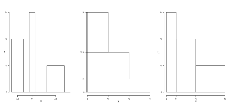
Figure 1: Simple function $f$ (left), its distribution function $m$ (middle) and decreasing rearrangement $f_{\downarrow}$ (right)

Using the decreasing rearrangement we can give the following definitions.

Definition 2.5.

Let $f$ and $g$ be density functions on the interval $(0,1)$. Then $g$ has more information than $f$, write $f\prec g$, if

$$\int_{0}^{u}f_{\downarrow}(v)dv\leq\int_{0}^{u}g_{\downarrow}(v)dv,\ \ \mbox{for all $u\in(0,1)$}$$

Definition 2.6.

Let $\mathcal{F}_{(0,1)}$ be the set of density functions $f$ on the interval $(0,1)$. Then $M_{(0,1)}:\mathcal{F}_{(0,1)}\to\mathbb{R}$ is an information measure if it is monotone with respect to the partial ordering in Definition 2.5

The distribution with minimum information is the uniform distribution on $(0,1)$. Information measures are easily found, see [28], as $f\prec g$ if and only if

$$\int_{0}^{1}C(f(u))du\leq\int_{0}^{1}C(g(u))du\ \ \mbox{for all continuous convex functions $C$}$$

[28] also discusses how to construct linear operators $L$ for which $f=Lg\prec g$ when $f\prec g$.

Consider next a continuous random variable $x$ on $\mathbb{R}$ with pdf $f$. To find a location and scale-free version of the density, [31] proposed the transformation

$$f(x),\ x\in\mathbb{R}\ \ \to\ \ f^{*}(u)=\frac{f(F^{-1}(u))}{H^{*}(x)},\ u\in(0,1).$$

Then $f^{*}$, called the probability density quantile (pdQ), is a probability density function on $(0,1)$ which is invariant under linear transformations of the original variable $x$ [31]. It is also true that, for given $f^{*}$, the original $f$ is known up location and scale. Using this density transformation, the definition of an invariant information measure for densities on $\mathbb{R}$ can be given as follows.

Definition 2.7.

Let $\mathcal{F}_{\mathbb{R}}$ be a set of density functions $f$ on $\mathbb{R}$ and let $M_{(0,1)}:\mathcal{F}_{(0,1)}\to\mathbb{R}$ be an information measure for distributions on $(0,1)$. Then $M_{\mathbb{R}}:f\to M_{(0,1)}(f^{*})$ is an information measure in the set $\mathcal{F}_{\mathbb{R}}$.

Note that $M_{\mathbb{R}}$ is not an extension of $M_{(0,1)}$ meaning that, $f\in\mathcal{F}_{(0,1)}$ does not imply that $M_{\mathbb{R}}(f)=M_{(0,1)}(f)$. $M_{\mathbb{R}}$ is invariant under rescaling of $f$ while $M_{(0,1)}$ is not.

Applying Definition 2.7 and choosing convex $C(u)=-log(u)$ and $C(u)=log(u)u$, we get location and scale invariant information measures for $f$ such as

$$\exp\{-2\int\log(f^{*}(u))du\}=e^{2H(x)}[H^{*}(x)]^{2}$$

and

$$\exp\{4\int\log(f^{*}(u))f^{*}(u)du\}\ =e^{-2H(f^{2}/H^{*}(x))}[H^{*}(x)]^{-2},$$

which attain their minimum at the uniform distribution and are invariant under the transformations $f\to f_{a,b,\Delta}$. For more details see e.g. [32].

To replace the transformation $f\to f^{*}$ by a transformation to densities on $(0,1)$ for which minimum information is attained at any density $g$, one can use the following adjustment.

Theorem 2.3.

Let $x$ and $y$ be random variables on $\mathbb{R}$ with the probability density functions $f$ and $g$ and cumulative distribution functions $F$ and $G$, respectively. Then

$$f:g(u)=\frac{f(G^{-1}(u))}{g(G^{-1}(u))}$$

is a density function on $(0,1)$ and its differential entropy is $-H(f:g)\geq 0$ is the Kullback-Leibler (KL) divergence between the distributions of $x$ and $y$.

Let again $x$ have a density $f$ and let $\varphi$ and $\Phi$ be the pdf and the cdf of a normal distribution with mean $E(x)$ and variance $Var(x)$. Then one can show, using similar arguments as in [31], that

$$f:\varphi(u)=\frac{f(\Phi^{-1}(u))}{\varphi(\Phi^{-1}(u))},\ \ u\in(0,1)$$

is a location and scale-free density and information measures in Definition 2.6 applied to the set of densities $\tilde{f}=f:\varphi$ attain their minimums when $f$ has a normal distribution. A collection of information measures is given by $\int C(\tilde{f}(u))du$ with continuous and convex functions $C$ and then we get for example again

$$\exp\{2\int log(\tilde{f}(u))\tilde{f}(u)du\}=(2\pi e)e^{-2H(x)}Var(x).$$

We next provide examples on the probability density functions $f$, $f^{*}$ and $\tilde{f}$ when $f$ is the density of Gaussian, Laplace, Lognormal and Uniform distributions. Also a mixture of two Gaussian distributions denoted by $GMM(\mu_{1},\mu_{2},\sigma_{1},\sigma_{2},w)$ is considered with the densities $w\varphi_{\mu_{1},\sigma_{1}}(x)+(1-w)\varphi_{\mu_{2},\sigma_{2}}(x)$, $0\leq w\leq 1$. Figure 2 then shows the impact of the transformations $f\to f^{*}$ and $f\to\tilde{f}$ in these cases.

Table 1: The power entropy and the $[H^{*}]^{-2}$ measure for some continuous distributions and their transformations.

Distribution	$e^{2H(f)}$	$e^{2H(f^{*})}$	$e^{2H(\tilde{f})}$		$H^{*}(f)^{-2}$	$H^{*}(f^{*})^{-2}$	$H^{*}(\tilde{f})^{-2}$
N(0,1)	17.079	0.824	1.000		12.566	0.750	1.000
Laplace(1)	29.556	0.680	0.887		16.000	0.719	0.783
Lognormal(0,1)	17.079	0.642	0.308		7.622	0.537	0.186
U(0,1)	1.000	1.000	0.703		1.000	1.000	0.567
GMM($0,4,1,2,0.4$)	100.000	0.862	0.855		78.000	0.792	0.756

Table LABEL:t1 provides for the same distributions the power entropies $e^{2H(\cdot)}$ and $H^{*}(\cdot)^{-2}$ for $f$, $f^{*}$ and $\tilde{f}$. Note that the information measures applied to $f$ are not invariant under rescaling of $x$ as opposed to $f^{*}$ and $\tilde{f}$. For example for the settings we use in the Table LABEL:t1, the normal and lognormal densities have the same power entropy just by accident and the equality is not generally true.

Figure 2: Comparison of $f$, $f^{*}$ and $\tilde{f}$ for five distributions.

For better understanding on the measures, we illustrate the behavior of $e^{H(\cdot)}$ and $H^{*}(\cdot)^{-2}$ in the GMM model with four fixed and one varying parameter, each in turn. In Figure 3 both information measure curves are plotted in the same figures to compare the shapes of the curves as well as the occurrences of extreme values. The curves for $\tilde{f}$ with varying location and scale seem natural as minimum information is attained as GMM gets “closer” to the normal distribution. Results for $f^{*}$ and varying location seem strange in a sense where one would expect decreasing behaviour of both measures as the distance in means increases, as it is case for $\tilde{f}$, while the result for $f$ in all three cases could simply be explained with decrease in information as a result of increase in overall variance of the mixture. $e^{H(\cdot)}$ and $H^{*}(\cdot)^{-2}$ seem to behave almost proportionally in all cases. In cases of $f^{*}$ and $\tilde{f}$ where the majorization is well defined, such behaviour is indeed expected, as the reciprocals of both $e^{H(\cdot)}$ and $H^{*}(\cdot)^{-2}$ are information measures for both $f^{*}$ and $\tilde{f}$. However, further investigations into this matter will be conducted in the future.

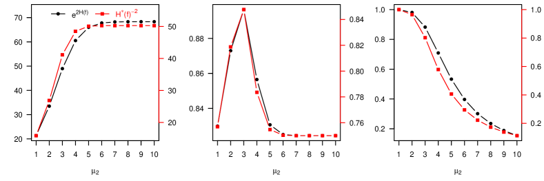
(a) GMM($0,\mu_{2},1,1,0.5$) where $\mu_{2}$ varies.

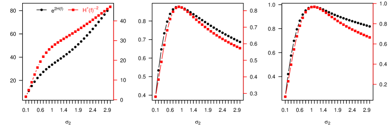
(b) GMM($0,2,1,\sigma_{2},0.5$) where $\sigma_{2}$ varies.

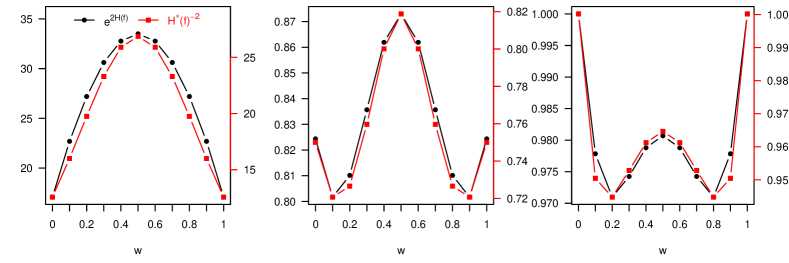
(c) GMM($0,2,1,1,w$) where $w$ varies.

Figure 3: Power entropy and $[H^{*}]^{-2}$ for different GMMs when always one parameter varies. The left vertical axis corresponds to power entropy and the right axis to $[H^{*}]^{-2}$. The left panel gives the measures for $f$, the middle for $f^{*}$ and the right for $\tilde{f}$.

3 Independent component analysis

3.1 Some preliminaries

In this section we consider multivariate random variables. For a $p$-variate random vector $\mathbf{x}$ with finite second moments, the mean vector and covariance matrix are $E(\mathbf{x})\in\mathbb{R}^{p}$ and $Cov(\mathbf{x})\in\mathbb{R}^{p\times p}$, respectively. Let $Cov(\mathbf{x})=\mathbf{U}\mathbf{D}\mathbf{U}^{\prime}$ be the eigenvector-eigenvalue decomposition of the covariance matrix. Then $Cov(\mathbf{x})^{-1/2}:=\mathbf{U}\mathbf{D}^{-1/2}\mathbf{U}^{\prime}$ and $\mathbf{x}^{st}=Cov(\mathbf{x})^{-1/2}(\mathbf{x}-E(\mathbf{x}))$ standardizes $\mathbf{x}$, that is, $E(\mathbf{x}^{st})=\mathbf{0}$ and $Cov(\mathbf{x}^{st})=\mathbf{I}_{p}$. The set of $p\times r$, $r\leq p$, matrices with orthonormal columns is denoted by $\mathcal{O}^{p\times r}$. Thus $\mathbf{U}\in\mathcal{O}^{p\times r}$ implies $\mathbf{U}^{\prime}\mathbf{U}=\mathbf{I}_{r}$. The set of $p\times p$ diagonal matrices with positive diagonal elements is denoted by $\mathcal{D}^{p\times p}$. If $\mathbf{U}\in\mathcal{O}^{p\times p}$ and $\mathbf{D}\in\mathcal{D}^{p\times p}$ then $\mathbf{x}\to\mathbf{U}\mathbf{x}$ and $\mathbf{x}\to\mathbf{D}\mathbf{x}$, $\mathbf{x}\in\mathbb{R}^{p}$, are a rotation operator and a componentwise rescaling operator, respectively. Let $\mathbf{A}\in\mathbb{R}^{p\times q}$ be a matrix with rank $r\leq\min\{p,q\}$. Then the linear operator $\mathbf{A}$ may be written as (singular value decomposition, SVD) $\mathbf{A}=\mathbf{U}\mathbf{D}\mathbf{V}^{\prime}=\sum_{i=1}^{r}d_{i}\mathbf{u}_{i}\mathbf{v}_{i}^{\prime}$ where $\mathbf{U}=(\mathbf{u}_{1},...,\mathbf{u}_{r})\in\mathcal{O}^{p\times r}$, $\mathbf{V}=(\mathbf{v}_{1},...,\mathbf{v}_{r})\in\mathcal{O}^{q\times r}$, and $\mathbf{D}\in\mathcal{D}^{r\times r}$.

3.2 Elliptical model and independent components model

Let $\mathbf{x}$ be a $p$-variate vector with the full-rank covariance matrix $Cov(\mathbf{x})$. We say that $\mathbf{x}$ has a spherical distribution if there exists a $\boldsymbol{\mu}$ such that $(\mathbf{x}-\boldsymbol{\mu})\sim\mathbf{U}(\mathbf{x}-\boldsymbol{\mu})$ for all orthogonal $\mathbf{U}$. In the following we first define the elliptic and independent components distributions (see for example [23, 24] for more details).

Definition 3.1.

Let $\mathbf{x}\in\mathbb{R}^{p}$ be a $p$-variate random vector.

1. $\mathbf{x}$ has an elliptical distribution if there exists a nonsingular $\mathbf{A}\in\mathbb{R}^{p\times p}$ such that $\mathbf{A}\mathbf{x}$ has a spherical distribution.

2. $\mathbf{x}$ has an independent components distribution if there exists a nonsingular $\mathbf{A}\in\mathbb{R}^{p\times p}$ such that $\mathbf{A}\mathbf{x}$ has independent components.

We next provide some results on how the matrix $\mathbf{A}$ can be found in different cases.

Theorem 3.1.

Let $\mathbf{x}$ be a $p$-variate random vector with a full-rank covariance matrix $Cov(\mathbf{x})=\mathbf{U}\mathbf{D}\mathbf{U}^{\prime}$. Then we have the following.

1. $[\mathbf{V}\mathbf{D}^{-1/2}\ \mathbf{U}^{\prime}]\mathbf{x}$ has uncorrelated components for all orthogonal $\mathbf{V}$.

2. If $\mathbf{x}$ has an elliptical distribution, $[\mathbf{V}\mathbf{D}^{-1/2}\ \mathbf{U}^{\prime}]\mathbf{x}$ has a spherical distribution for all orthogonal $\mathbf{V}$.

3. If $\mathbf{x}$ has an independent components distribution, $[\mathbf{V}\mathbf{D}^{-1/2}\ \mathbf{U}^{\prime}]\mathbf{x}$ has independent components for some choice(s) of orthogonal $\mathbf{V}$.

4. If $\mathbf{x}$ has both an elliptical distribution and an independent component distribution then $[\mathbf{V}\mathbf{D}^{-1/2}\ \mathbf{U}^{\prime}]\mathbf{x}$ has independent Gaussian components for all orthogonal $\mathbf{V}$, that is, $\mathbf{x}$ has a multivariate Gaussian distribution.

3.3 Projection pursuit and independent component analysis

Let $\mathbf{x}$ have an independent components distribution such that $\mathbf{z}=\mathbf{A}\mathbf{x}+\mathbf{b}$ is standardized ($E(\mathbf{z})=\mathbf{0}$ and $Cov(\mathbf{z})=\mathbf{I}_{p}$) and has independent components. Theorem 3.1 then implies that $\mathbf{A}=\mathbf{V}^{\prime}Cov(\mathbf{x})^{-1/2}$ where the rotation matrix $\mathbf{V}$ can be chosen as $\mathbf{V}=(\mathbf{V}_{1},\mathbf{V}_{2})$ separating non-Gaussian independent components in $\mathbf{V}_{1}^{\prime}Cov(\mathbf{x})^{-1/2}\mathbf{x}$ and Gaussian independent components in $\mathbf{V}_{2}^{\prime}Cov(\mathbf{x})^{-1/2}\mathbf{x}$. Note that $\mathbf{V}_{2}$ is only unique up to right multiplication by an orthogonal matrix. A generally accepted strategy is to find $\mathbf{V}_{1}=(\mathbf{v}_{1},...,\mathbf{v}_{q})\in\mathcal{O}^{p\times q}$ such that the components of $\mathbf{V}_{1}^{\prime}\mathbf{x}^{st}$ are as ‘non-Gaussian as possible’. The Gaussian part $\mathbf{V}_{2}^{\prime}Cov(\mathbf{x})^{-1/2}\mathbf{x}$ is thought to be just the noise part and, for other components, it is argued that the sum of independent random variables is ‘more Gaussian’ than the original variables. The noise interpretation of the Gaussian part may be motivated by the following. A random vector has a multivariate normal distribution if and only if all linear combinations of the marginal variables have univariate normal distributions, that is, there are no ‘interesting’ directions. The normal distribution is the only distribution for which all third and higher cumulants are zero. As seen before, a Gaussian distribution is the distribution with the poorest information among distributions with the same variance (highest entropy, smallest Fisher information).  For a thorough discussion of Gaussian distributions, see [14].

Let $D(x)$ then be the projection index, i.e., the functional that is used to measure non-Gaussianity. In the one-by-one projection pursuit approach the first direction $\mathbf{v}_{1}$ ($\mathbf{v}_{1}^{\prime}\mathbf{v}_{1}=1$) maximizes $D(\mathbf{v}_{1}^{\prime}\mathbf{x}^{st})$, the second direction $\mathbf{v}_{2}$ is orthogonal to $\mathbf{v}_{1}$ ($\mathbf{v}_{2}^{\prime}\mathbf{v}_{2}=1,\mathbf{v}_{2}^{\prime}\mathbf{v}_{1}=0$) and maximizes $D(\mathbf{v}_{2}^{\prime}\mathbf{x}^{st})$ and so on. After finding $\mathbf{v}_{1},...,\mathbf{v}_{j-1}$, we optimize the Lagrangian function

$$L(\mathbf{v};\lambda_{j1},...,\lambda_{jj})=D(\mathbf{v}^{\prime}\mathbf{x}^{st})-\lambda_{jj}(\mathbf{v}^{\prime}\mathbf{v}-1)-\sum_{i=1}^{j-1}\lambda_{ji}\mathbf{v}^{\prime}\mathbf{v}_{i}.$$

Then $\mathbf{v}_{j}$ solves the (estimating) equation $(\mathbf{I}_{p}-\sum_{i=1}^{j-1}\mathbf{v}_{i}\mathbf{v}_{i}^{\prime})\mathbf{T}(\mathbf{v})=(\mathbf{T}(\mathbf{v})^{\prime}\mathbf{v})\mathbf{v},$ where $\mathbf{T}(\mathbf{v})=\partial D(\mathbf{v}^{\prime}\mathbf{x}^{st})/\partial\mathbf{v}$. From the computational point of view, this suggests a fixed-point algorithm. The estimation equation also provides a way to find the limiting distribution of the estimate, since the estimate is obtained when the theoretical multivariate distribution is replaced by the empirical one. See for example [20, 21, 22] and references therein for more details.

The following questions naturally arise. How should one choose the projection index $D(x)$ to find the independent components? Are the independent components provided by the most informative directions as has been often stated in the literature? These questions are partially answered by the following.

Theorem 3.2.

Let $\mathbf{z}=\mathbf{A}\mathbf{x}+\mathbf{b}=(z_{1},...,z_{p})^{\prime}$ be the vector of standardized independent components.

1. Let $D(x)$ be a subadditive squared dispersion measure.
   Then $D(\mathbf{v}^{\prime}\mathbf{x}^{st})\leq\max_{j}D(z_{j})$.

2. Let $D(x)$ be a superadditive squared dispersion measure.
   Then $D(\mathbf{v}^{\prime}\mathbf{x}^{st})\geq\min_{j}D(z_{j})$.

Based on Theorem 3.2 and the discussion above we can now end the paper with the following conclusions. If $D(x)$ is subadditive then it can be used as a projection index. For example the cumulants $\kappa_{2k+1}^{2/(2k+1)}(x)$ and $\kappa_{2k+2}^{2/(2k+2)}(x)$, $k=1,2,\ldots$, when calculated for standardized distributions, provide squared dispersion measures that are subadditive. Therefore they can be used as projection indices. For superadditive $D(x)$, the functional $(D(x))^{-1}$ is a valid projection index as $(D(\mathbf{v}^{\prime}\mathbf{x}^{st}))^{-1}\leq\max_{j}(D(z_{j}))^{-1}$. As seen before, entropy power $e^{H(x)}$ and the inverse of Fisher information, $J^{-1}(x)$ are superadditive squared dispersion measures. Note that in both cases $D(\mathbf{v}^{\prime}\mathbf{x}^{st})$ is in fact a ratio of two squared dispersion functions, and the projection index measures deviation from Gaussianity using a skewness, kurtosis or information measure. As mentioned in Section 3.3, $(\kappa_{3}^{2}(x)+(1/4)\kappa_{4}^{2}(x))/12$ provides an approximation of negative differential entropy in a neighborhood of Gaussian distribution and is a valid projection index as well. For further discussion, see [10]. Note also that one of the most popular ICA procedures in the engineering community, the so called fastICA, uses a projection index of the form $D(x)=|E[C(x)])|$ where $C$ is such a function that, if $z\sim N(0,1)$ then $E[C(z)]=0$. Examples of valid choices of $C$ are $C(z)=z^{3}$ and $C(z)=z^{4}-3$ providing again the third and fourth cumulants, respectively.

4 Final remarks

The usage of various information criteria is popular in independent component analysis. The connections between notions of information and statistical independence and the special role of the Gaussian distribution were discussed in detail in the paper. We also introduced new ideas and partial orderings for information which utilize transformed location and scale-free probability density functions. In independent component analysis with unknown marginal densities, the estimation of the value of the adapted information measure in a given direction is highly challenging and it has to be done again and again when applying the fixed point algorithm for the correct direction. Substantial research is therefore still needed for these tools to be of practical value.

5 Appendix: The Proofs

Proof of Theorem 2.1. Let $x_{1},...,x_{n}$ be a random sample from a distribution of $x$ with the mean value $E(x)$ and variance $Var(x)$. By the central limit theorem,

$$z_{n}=\frac{1}{\sqrt{n}}\sum_{i=1}^{n}\frac{x_{i}-E(x)}{\sqrt{Var(x)}}\to_{d}z\sim N(0,1).$$

Therefore, by additivity and affine equivariance,

$$T(z_{n})=\sqrt{\frac{n}{Var(x)}}(T(x)-E(x))\to 0\ \ \mbox{and}\ \ S^{2}(z_{n})=\frac{S^{2}(x)}{Var(x)}\to S^{2}(z)$$

and the result follows. For similar results in the multivariate case, see [34].

Proof of Theorem 2.2. The invariances of the measures $H(x)$, $H^{*}(x)$, $H^{**}(x)$ and $J(x)$ under location shifts $f(x)\to f(x+b)$, sign change $f(x)\to f(-x)$ as well as under $f\to f_{a,b,\Delta}$ follow easily from their definitions and from the definition of the Riemann integral. We therefore only have to consider rescaling $f(x)\to(1/a)f(x/a)$ with $a>0$. Then $H(ax)=-\int(1/a)f(x/a)\log((1/a)f(x/a))dx=-\int f(x)\log((1/a)f(x))dx=H(x)+\log(a)$ and therefore $e^{2H(ax)}=a^{2}e^{H(x)}$. In a similar way one can show that $[H^{*}(ax)]^{-2}=a^{2}[H^{*}(x)]^{-2}$. Also easily $[H^{**}(ax)]^{-2}=a^{2}[H^{**}(x)]^{-2}$. As $f^{\prime}(x)\to(1/a^{2})f^{\prime}(x/a)$ one also easily shows that $[J(ax)]^{-1}=a^{2}[J(x)]^{-1}$. Thus all the four measure are scale equivariant and therefore squared dispersion measures.

Proof of Theorem 2.3. $f:g$ is indeed a density function since it is trivially nonnegative and $\int_{0}^{1}(f:g)(u)\mathrm{d}u=\int_{0}^{1}\frac{f(G^{-1}(u))}{g(G^{-1}(u))}\mathrm{d}u=\int_{-\infty}^{\infty}f(x)\mathrm{d}x=1$ with the substitution $x=G^{-1}(u)$. Similary, $-H(f:g)=\int_{0}^{1}(f:g)(u)\log((f:g)(u))\mathrm{d}u=\int_{-\infty}^{\infty}f(x)\log\frac{f(x)}{g(x)}\mathrm{d}x=D(f||g).$

Proof of Theorem 3.1. (1) Let $\mathbf{V}$ be orthogonal. As $Cov([\mathbf{V}\mathbf{D}^{-1/2}\mathbf{U}^{\prime}]\mathbf{x})=\mathbf{V}\mathbf{D}^{-1/2}\mathbf{U}^{\prime}Cov(\mathbf{x})\mathbf{U}\mathbf{D}^{-1/2}\mathbf{V}^{\prime}=\mathbf{V}\mathbf{V}^{\prime}=\mathbf{I}_{p}$, the components of $[\mathbf{V}\mathbf{D}^{-1/2}\mathbf{U}^{\prime}]\mathbf{x})$ are uncorrelated. (2) Assume that $\mathbf{A}\mathbf{x}$ is spherical with $\mathbf{A}=\mathbf{V}\mathbf{C}\mathbf{W}^{\prime}$ rescaled so that $Cov(\mathbf{A}\mathbf{x})=\mathbf{I}_{p}$. As $\mathbf{A}Cov(\mathbf{x})\mathbf{A}^{\prime}=\mathbf{I}_{p}$, $Cov(\mathbf{x})=(\mathbf{A}^{\prime}\mathbf{A})^{-1}$ and $\mathbf{W}\mathbf{C}^{-2}\mathbf{W}^{\prime}=\mathbf{U}\mathbf{D}\mathbf{U}^{\prime}$. Therefore $\mathbf{W}=\mathbf{U}$ and $\mathbf{C}=\mathbf{D}^{-1/2}$ and we can conclude that $[\mathbf{V}\mathbf{D}^{-1/2}\mathbf{U}^{\prime}]\mathbf{x}$ is spherical for any orthogonal $\mathbf{V}$. (If $\mathbf{x}$ is spherical then $\mathbf{V}\mathbf{x}$ is spherical for all orthogonal $\mathbf{V}$.) (3) Let $\mathbf{A}\mathbf{x}$ with $\mathbf{A}=\mathbf{V}\mathbf{C}\mathbf{W}^{\prime}$ have independent and standardized components so that $Cov(\mathbf{A}\mathbf{x})=\mathbf{I}_{p}$. As in (2), $\mathbf{A}$ must be $\mathbf{V}\mathbf{D}^{-1/2}\mathbf{U}^{\prime}$ but now for some $\mathbf{V}$ only. (It is not true that if $\mathbf{x}$ has independent standardized components then $\mathbf{V}\mathbf{x}$ has independent components for any choice of $\mathbf{V}$.) (4) Based on (2) and (3), there exist an $\mathbf{A}=\mathbf{V}\mathbf{D}^{-1/2}\mathbf{U}^{\prime}$ such that $\mathbf{A}\mathbf{x}$ has a spherical distribution with independent components. Then by the Maxwell-Hershell theorem, $\mathbf{A}\mathbf{x}$ has a multivariate normal distribution. For the proof of the Maxwell-Hershell theorem, see e.g. Proposition 4.11. in [5].

Proof of Theorem 3.2. Let $\mathbf{z}=\mathbf{A}\mathbf{x}+\mathbf{b}=(z_{1},...,z_{p})^{\prime}$ be a vector of standardized independent components. By Theorem 3.1, $\mathbf{z}=\mathbf{V}\mathbf{x}^{st}$ with some orthogonal $\mathbf{V}$. If $\mathbf{u}^{\prime}\mathbf{u}=1$ then also $(\mathbf{V}\mathbf{u})^{\prime}(\mathbf{V}\mathbf{u})=1$ and therefore $D(\mathbf{u}^{\prime}\mathbf{x}^{st})=D(\mathbf{u}^{\prime}\mathbf{V}\mathbf{z})\leq\sum(\mathbf{V}^{\prime}\mathbf{u})_{i}^{2}D(z_{i})\leq\max_{j}D(z_{j})$ for subadditive squared dispersion measure $D$ and $D(\mathbf{u}^{\prime}\mathbf{x}^{st})=D(\mathbf{u}^{\prime}\mathbf{V}\mathbf{z})\geq\sum(\mathbf{V}^{\prime}\mathbf{u})_{i}^{2}D(z_{i})\geq\min_{j}D(z_{j})$ for superadditive squared dispersion measure $D$.

6 Acknowledges

The work of KN has been supported by the Austrian Science Fund (FWF) Grant number P31881-N32.

References

- [1] A. R. Barron: Entropy and the central limit theorem. Ann. Probab. 14 (1986), 336–342.
- [2] A. J. Bell, T. J. Sejnowski: An information-maximization approach to blind separation and blind deconvolution. Neural Comput. 7 (1995), 1129–1159.
- [3] P. J. Bickel, E. L. Lehmann: Descriptive statistics for nonparametric models II: Location. Ann. Stat. 3 (1975), 1045–1069.
- [4] P. J. Bickel, E. L. Lehmann: Descriptive statistics for nonparametric models III: Dispersion. Ann. Stat. 4 (1976), 1139–1158.
- [5] M. Bilodeau, D. Brenner: Theory of multivariate statistics. Springer Texts in Statistics. New York: Springer (1999).
- [6] H. Chernoff, I. R. Savage: Asymptotic normality and efficiency of certain nonparametric test statistics. Ann. Math. Stat. 29 (1958), 972–994.
- [7] T. Cover, J. Thomas: Elements of information theory. New York: John Wiley & Sons. (1991).
- [8] L. Faivishevsky, J. Goldberger: ICA based on a smooth estimation of the differential entropy. Advances in Neural Information Processing Systems 21 (2008), 433–440.
- [9] J. L. Hodges, E. L. Lehmann: The efficiency of some nonparametric competitors of the t-test. Ann. Math. Stat. 27 (1956), 324–335.
- [10] P. J. Huber: Projection pursuit. Ann. Stat. 13 (1985), 435–475.
- [11] A. Hyvärinen: New approximations of differential entropy for independent component analysis and projection pursuit. Advances in Neural Information Processing Systems, 10 (1998), 273–279.
- [12] A. Hyvärinen, J. Karhunen, E. Oja: Independent component analysis. John Wiley & Sons, New York (2001)
- [13] M. C. Jones, R. Sibson: What is projection pursuit? J. R. Stat. Soc., Ser. A 150, (1987), 1–36.
- [14] K. Kim, G. Shevlyakov: Why Gaussianity? IEEE Signal Process. Mag. 25 (2008), 102–113.
- [15] E. Kristiansson: Decreasing Rearrangement and Lorentz L(p,q) Spaces (Thesis). Department of Mathematics of the Lulea University of Technology, (2002). Available at: http://citeseerx.ist.psu.edu/viewdoc/download?doi=10.1.1.111.1244&rep=rep1&type=pdf.
- [16] S. Kullback: Information theory and statistics. John Wiley and Sons, Inc., New York; Chapman and Hall, Ltd., London 1959.
- [17] E. G. Learned-Miller, J. W. Fisher III: ICA using spacings estimates of entropy. J. Mach. Learn. Res. 4 (2004), 1271–1295.
- [18] B. G. Lindsay, W. Yao: Fisher information matrix: A tool for dimension reduction, projection pursuit, independent component analysis, and more. Can. J. Statistics 40 (2012), 712–730.
- [19] A. W. Marshall, I. Olkin: Inequalities: Theory of majorization and its applications. Mathematics in Science and Engineering, Vol. 143. Academic Press, New York, 1979.
- [20] J. Miettinen, K. Nordhausen, H. Oja, S. Taskinen: Deflation-based FastICA with adaptive choices of nonlinearities. IEEE Trans. Signal Process. 62 (2014), 5716–5724.
- [21] J. Miettinen, K. Nordhausen, H. Oja, S. Taskinen: Fourth moments and independent component analysis. Stat. Sci. 30 (2015), 372–390.
- [22] J. Miettinen, K. Nordhausen, H. Oja, S. Taskinen, J. Virta: The squared symmetric fastICA estimator. Signal Process. 131 (2017), 402–411.
- [23] K. Nordhausen, H. Oja: Independent component analysis: a statistical perspective. Wiley Interdiscip. Rev. Comput. Stat. 10 (2018), e1440.
- [24] K. Nordhausen, H. Oja: Robust nonparametric inference. Annu. Rev. Stat. Appl. 5 (2018), 473–500.
- [25] H. Oja: On location, scale, skewness and kurtosis of univariate distributions. Scand. J. Stat. 8 (1981), 154–68.
- [26] E. Parzen: Quantile probability and statistical data modeling. Statist. Sci. 19 (2004), 652–662.
- [27] J. E. Pečarić, F. Proschan, Y. L. Tong: Convex functions, partial orderings, and statistical applications. Mathematics in Science and Engineering, 187. Academic Press, Boston, 1992.
- [28] J. V. Ryff: On the representation of doubly stochastic operators. Pacific J. Math. 13 (1963), 1379–1386.
- [29] R. Serfling: Asymptotic relative efficiency in estimation. International Encyclopedia of Statistical Science. Springer (2011), 68–72.
- [30] C. E. Shannon: A mathematical theory of communication. The Bell System Technical Journal, 27 (1948), 379–423.
- [31] R. G. Staudte: The shapes of things to come: probability density quantiles. Statistics, 51 (2017), 782–800.
- [32] R. G. Staudte, A. Xia: Divergence from, and convergence to, uniformity of probability density quantiles. Entropy, 20 (2018), Paper No. 317, 10.
- [33] V. Vigneron, C. Jutten: Fisher information in source separation problems. Lecture Notes in Computer Science 3195 (2004), 168–176.
- [34] J. Virta: On characterizations of the covariance matrix. (2018), Preprint available as arXiv:1810.01147.
- [35] J. Virta, K. Nordhausen: On the optimal nonlinearities for gaussian mixtures in FastICA. Latent Variable Analysis and Signal Separation. 13th International Conference, LVA/ICA 2017, Grenoble, France, February 21-23, 2017, Proceedings, 427–437.
- [36] W. R. van Zwet: Convex transformations of random variables. Mathematical Centre Tracts, Mathematisch Centrum, Amsterdam, 1964.