A general framework for defining and optimizing robustness

Abstract

Robustness of neural networks has recently attracted a great amount of interest. The many investigations in this area lack a precise common foundation of robustness concepts. Therefore, in this paper, we propose a rigorous and flexible framework for defining different types of robustness properties for classifiers. Our robustness concept is based on postulates that robustness of a classifier should be considered as a property that is independent of accuracy, and that it should be defined in purely mathematical terms without reliance on algorithmic procedures for its measurement. We develop a very general robustness framework that is applicable to any type of classification model, and that encompasses relevant robustness concepts for investigations ranging from safety against adversarial attacks to transferability of models to new domains. For two prototypical, distinct robustness objectives we then propose new learning approaches based on neural network co-training strategies for obtaining image classifiers optimized for these respective objectives.

1 Introduction

Machine learning models have reached impressive levels of performance for solving various types of classification problems. Famously, convolutional neural networks [7, 18], are the state-of-the-art method for image classification (see, e.g., [33, 39, 16]). However, the phenomenon of adversarial examples [32, 8] has raised serious concerns about the reliability of these machine learning solutions, especially in safety-critical applications. Autonomous driving and counterfeit bill detection are two intuitive examples where safety concerns play a fundamental role. The vulnerability of machine learning models to adversarial examples is widely interpreted as a lack of robustness of these models, and a large amount of recent work investigates robustness properties, with a strong focus on deep neural network models. Research in this area has been pursued both from the perspective of formal verification with its traditional objective of rigorously proving safety properties of hard- and software systems [26, 4, 3, 1, 2, 37], and from the perspective of machine learning with its traditional objective of optimizing expected values of performance measures [21, 11, 5, 28, 31].

The original motivation derived from adversarial examples led to a focus on robustness against small adversarial perturbations. As noted by [6], this needs to be distinguished from robustness under larger scale distribution shifts. The former is a particular concern in order to guard against vulnerability to targeted attacks, whereas the latter is important for applications where the characteristics of test cases may (eventually) differ from the original training data.

In most works, the focus is on one of two separate issues: either assessing the robustness properties of a given model, or improving the robustness properties of learned classifiers by developing new training techniques. Works with a background in formal verification mostly focus on the first issue, while in the field of machine learning the second plays a larger role. However, in machine learning, too, the problem of assessing robustness has received a lot of attention, especially in connection with designing adversarial attacks [8, 21, 11, 31].

The underlying concept of robustness used in different works often only is implicit in a proposed loss function and/or the experimental protocol used to evaluate robustness properties. As a result, there does not yet appear to be a common full understanding of what robustness actually is, and how it relates to other properties of classification models. For example, [35] have argued that the objectives of robustness and accuracy are in conflict with each other, whereas [29] come to somewhat opposite conclusions: they argue that robustness and generalization capabilities are in conflict only when robustness is designed to defend against “off-manifold” attacks, i.e., adversarial examples that do not follow the data distribution, whereas they are consistent with each other in the scenario of “on-manifold” adversarial examples. Similarly, there exist somewhat conflicting results with regard to the question whether robustness against adversarial examples and against distribution shifts are in conflict with each other, or whether these two objectives can be aligned [6, 27].

Underlying these differences are not so much theoretical or empirical discrepancies, as conceptual differences about what one wants to capture with robustness. In this paper we first aim to put the analysis of robustness properties on a more solid foundation by developing a general framework for the specification of different robustness concepts that captures most of the concepts previously used (implicitly or explicitly) in the literature, and that helps to clarify their basic structural differences. We propose a flexible framework that captures in a coherent manner different robustness concepts ranging from safety against adversarial attacks to the ability to adapt to distribution changes. In this manner, we draw a direct link between the goals of learning robust and safe classifiers on the one hand, and the traditional objectives of transfer learning on the other hand.

We then use our robustness definitions as the conceptual basis for developing robust learning techniques in two protypical application settings: learning neural network classifiers that are robust against small adversarial perturbations, and learning image classifiers that are robust with respect to larger distribution shifts. Like most of previous research on robustness which focusses on neural network technology for image classification problems, we, too, use readily available image benchmark datasets and standard neural network architectures to evaluate our methods. However, it is one of our core objectives that the conceptual framework is generally applicable to all types of classification models, and the developed techniques are not specifically tied to image data.

The key contributions of this paper are:

• A general analysis and specification framework for robustness concepts for classification models.

• Development of robust learning techniques for two prototypical instantiations of the robustness framework covering two very different points in the robustness spectrum.

2 A Robustness Framework

We are considering classification problems given by an input space $\mathcal{X}$, a label space $\mathcal{Y}=\{0,\ldots,K-1\}$, and a data distribution consisting of an input distribution $P(X)$, and a conditional label distribution $P(Y|X)$. A classifier is any mapping $f:\mathcal{X}\rightarrow\mathcal{Y}$. By as slight abuse of notation we also use $Y$ to denote the true labeling functions $Y:\mathcal{X}\rightarrow\mathcal{Y}$ defined by $Y(x):=\operatorname*{arg\,max}_{y}P(Y=y|X=x)$. Most existing notions of robustness require that $\mathcal{X}$ is endowed with a metric. Usually, ${\mathcal{X}}\subseteq\mathbb{R}^{d}$ for some $d\geq 1$, with a metric induced by one of the standard norms on $\mathbb{R}^{d}$. In the following we will assume that ${\mathcal{x}}$ is of this form.

Underlying our robustness framework are the following two postulates:

P1.

Robustness is orthogonal to accuracy (or generalization). In particular, a constant classifier with $f(x)=y$ for some fixed $y\in\mathcal{Y}$ and all $x\in\mathcal{X}$ always is maximally robust. This does not entail that robustness and accuracy are necessarily in conflict; only that they are separate, distinguishable objectives.

P2.

Robustness of a model $f$ is defined only in terms of $f$ itself, and the given classification problem. In particular, robustness is not dependent on specific (algorithmic) tools for assessing robustness.

P1 makes our concept of robustness different from robustness metrics used e.g. by [34] or [6], where robustness measures are directly tied to accuracy. These differences notwithstanding, the measures we propose are consistent with these earlier proposals in that they arguably extract their pure robustness components. P2 implies that e.g. success rates of particular adversarial example generators as used e.g. in [30], or the CLEVER scoring algorithm of [36] are not robustness measures in our sense per se, but rather tools for approximate evaluations of proper robustness measures.

P2 can be refined to a hierarchy of robustness concepts reflecting their dependence on different elements: we distinguish three types of robustness concepts, according to whether robustness is defined in terms of

Type 1:

only the classifier $f$,

Type 2:

the classifier $f$, and the input distribution $P(X)$

Type 3:

$f,P(X)$, and the label distribution $P(Y|X)$

We now develop a flexible framework that can accommodate a wide range of robustness concepts of all three types. In the following, ${\cal A}({\cal X})$ denotes the $\sigma$-algebra of Borel sets on ${\cal X}$.

Definition 1

(Basic $Q$-Robustness Measure) Let $f$ be a classifier and

$$\begin{array}[]{llll}Q:&{\cal X}\times{\cal A}({\cal X})&\rightarrow&[0,1]\\ &(x,A)&\mapsto&Q(A|x)\end{array}$$ (1)

a transition kernel on ${\cal X}$. The function

$$\begin{array}[]{rcl}\rho_{Q}^{f}:\ \ \mathcal{X}&\rightarrow&[0,1]\\ x&\mapsto&Q(\{x^{\prime}:f(x^{\prime})=f(x)\}|x)\end{array}$$ (2)

is called the basic robustness measure of $f$ with respect to $Q$.

In conjunction with a distribution $P()$ on ${\cal X}$, a kernel $Q$ defines the probability measure $\int_{\cal X}Q(\cdot|x)dP(x)$ on ${\cal X}$. We denote this measure as $Q\circ P$.

Example 1

Let $\epsilon>0$. We denote with $B_{\epsilon}(x)$ the open $\epsilon$-ball around $x$ (according to a chosen metric on ${\cal X}$). Let $Q_{\epsilon}(\cdot|x)$ be the uniform distribution on $B_{\epsilon}(x)$ ($x\in{\cal X}$). $\rho_{Q_{\epsilon}}^{f}(x)$ then is the probability that a perturbation of $x$ with a uniform random noise vector of length $\leq\epsilon$ is assigned by $f$ the same label as $x$.

The basic robustness measure measures the stability of the classifiers output when examples $x$ are randomly perturbed according to the distribution $Q(\cdot|x)$. Integrating $\rho_{Q}^{f}(x)$ over $x$ gives an overall robustness score for $f$ relative to $Q$-perturbations. However, simply taking the integral over $\rho_{Q}^{f}$ is too crude to encode many important versions of robustness. We therefore generalize the basic robustness measure by adding functions that allow to extract specific features of $\rho_{Q}^{f}$.

Definition 2

($Q,H,G$-Robustness Function) Let $H:[0,1]\rightarrow\mathbb{R}^{+}$ be a monotone increasing function, and $G:{\cal X}\rightarrow\mathbb{R}^{+}$. Then

$$\begin{array}[]{rcl}{\rho}_{Q,H,G}^{f}:\ \ \mathcal{X}&\rightarrow&\mathbb{R}^{+}\\ x&\mapsto&H(\rho_{Q}^{f}(x))G(x)\end{array}$$ (3)

is the robustness function of $f$ defined by $Q,H$ and $G$.

Integrating the robustness function then gives a robustness score for a classifier:

Definition 3

($Q,H,G$-Robustness Score) For a given $f$, $Q$, $H$, and $G$ we define the $Q,H,G$-robustness score

$$R_{Q,H,G}^{f}=\int_{\mathcal{X}}{\rho}^{f}_{Q,H,G}(x)dx.$$ (4)

We note that for a constant classifier $f(x)=i\in{\cal Y}\ (x\in{\cal X})$ we have $\rho^{f}_{Q}(x)=1$ for all $x$, and by the monotony of $H$ then also $H(\rho^{f}_{Q}(x))$ is the maximal possible value for all $x$. This implies that for all $Q,H,G$, $R_{Q,H,G}^{f}$ is maximal for a constant classifier, i.e., postulate P1 is satisfied.

The robustness score of Definition 3 only relates to a single perturbation model $Q$. Often, one will want to consider different forms of perturbations, possibly weighted by a probability distribution.

Definition 4

(${\cal Q},H,G$-Robustness Score) Let ${\cal Q}$ be a family of transition kernels $Q_{{\boldsymbol{\lambda}}}$ parameterized by ${\boldsymbol{\lambda}}\in A\subseteq\mathbb{R}^{k}$. Let ${\cal Q}$ be equipped with a probability distribution defined by a density function $q_{\cal Q}$ on $A$. Let $H$ and $G$ as in Definition 3. Then we define the ${\cal Q}$-robustness score as

$$R_{{\cal Q},H,G}^{f}=\int_{A}R_{Q_{{\boldsymbol{\lambda}}},H,G}^{f}q_{\cal Q}({\boldsymbol{\lambda}})d{\boldsymbol{\lambda}}.$$ (5)

We next illustrate how the general robustness concepts introduced by Definitions 1-4 can be instantiated to obtain previously proposed and novel robustness concepts of types 1-3. To simplify descriptions, from now on we assume that $\mathcal{X}$ is the $m$-dimensional unit hypercube, and we denote with $d=\sqrt{m}$ its diameter. In this paper, we will consider for $H$ only the two functions

$$\begin{array}[]{llll}H(p)&=&{\mathbf{1}}(p)&:={\mathbb{I}}[p=1],\ \ \mbox{and}\\ H(p)&=&{\mathit{i}d}(p)&:=p\end{array}$$

with ${\mathbb{I}}[\cdot]$ the indicator function. Thus, with $H={\mathbf{1}}$ we are only interested in whether the predicted label of $x$ will be almost surely preserved under the perturbation $Q(\cdot|x)$, which leads to robustness concepts related to safety guarantees under adversarial perturbations, wheras $H={\mathit{i}d}$ leads to robustness concepts concerned with preservation of predictive accuracy.

Example 2

(Geometry of decision regions; type 1.) For $\epsilon>0$ let $Q_{\epsilon}$ be defined as in Example 1. Define

$${\cal Q}_{[0,d]}:=\{Q_{\epsilon}|\epsilon\in[0,d]\}$$

and let $q_{{\cal Q}_{0}}$ be the uniform density on $[0,d]$. Let $H={\mathbf{1}}$, and $G(x)\equiv 1$. Under mild regularity conditions on $f$ we then have that

$${\mathbf{1}}(\rho^{f}_{Q_{\epsilon}}(x))={\mathbb{I}}[\forall x^{\prime}\in B_{\epsilon}(x):f(x^{\prime})=f(x)],$$ (6)

i.e. the probabilistic statement $Q_{\epsilon}(\ldots)=1$ can be sharpened into a categorical “for all” statement. Then

$$R^{f}_{{\cal Q}_{[0,d]},{\mathit{i}d},1}=\int_{0}^{d}\int_{\cal X}\rho^{f}_{Q_{\epsilon},{\mathbf{1}},1}(x)dxd\epsilon=\int_{\cal X}\int_{0}^{d}\rho^{f}_{Q_{\epsilon},{\mathbf{1}},1}(x)d\epsilon dx.$$ (7)

The inner integral on the right is equal to the minimum distance from $x$ to a decision boundary of $f$, i.e., the classifier margin at $x$. Integrating over ${\cal X}$ then gives that $R^{f}_{{\cal Q}_{[0,d]},{\mathit{i}d},1}$ is the average margin for points $x\in{\cal X}$. This robustness measure only depends on the geometric complexity of the decision regions of $f$.

Example 3

(Margin curves; type 2.)

Let ${\cal Q}_{[0,d]}$ be as in Example 2. Assume that $P(X)$ has a density function $p(x)$ relative to the uniform distribution, and let $G(x):=p(x)$. Then, under the same regularity assumptions as in Example 2, $R_{Q_{\epsilon},{\mathbf{1}},p}$ is the probability that a point $x$ sampled according to $P(X)$ has no adversarial example at distance $\leq\epsilon$. Empirical estimates of this integral based on a number of test points $x_{i}$ correspond to robustness scores in terms of success rates of adversarial example generators (where the precision of the estimate then also is affected by the effectiveness of the generator). Seen as a function of $\epsilon$, $R^{f}_{Q_{\epsilon},{\mathbf{1}},p}$ defines the margin curves of [9] (up to a $1-\ldots$ inversion). Integrating over $\epsilon\in[0,d]$ yields $R^{f}_{{\cal Q}_{[0,d]},{\mathbf{1}},p}$, which measures robustness as the area under the margin curve.

Example 4

(label aware; type 3.) Label-aware (type 3) robustness functions can be obtained by conditioning the perturbation distribution $Q_{\epsilon}(\cdot|x)$ also on the label of $x$. Thus we let

$$Q_{\epsilon,Y}(\cdot|x):=Q_{\epsilon}(\cdot|x)|\{x^{\prime}:Y(x^{\prime})=Y(x)\},$$

where we use the general notation $P|A$ to denote a probability distribution $P$ conditioned on an event $A\in{\cal A}({\cal X})$. With $H$ and $G$ as in Example 3, one now obtains the robustness concept implicitly (through the definition of the expected adversarial loss function) used in [35] and adapted in [9].

In all the preceding examples the data distribution $P(X)$ was only used to weigh the contribution of points $x\in{\cal X}$ to the overall robustness score. It was not used in the definition of the perturbation model ${\cal Q}$. The resulting robustness models then capture scenarios where datapoints generated by $Q\circ P$ can be off-manifold in the sense of [29]. For the more conservative setting of robustness with respect to on-manifold adversarial examples, one can also use $P()$ in the definition of $Q$ by letting

$$Q_{\epsilon,P}(\cdot|x):=P|B_{\epsilon}(x).$$

In all preceding examples, we can substitute $Q_{\epsilon,P}$ for $Q_{\epsilon}$, and thereby obtain on-manifold versions of the given robustness concepts. The question of whether an off-manifold or on-manifold concept of robustness is more appropriate is quite subtle. The former is more relevant when robustness against malicious attacks or substantial distribution changes is required; the latter may be sufficient when only robustness against distribution changes is required that are induced e.g. by changing observation biases, but do not modify the underlying nature of the sampling population.

None of the preceding definitions and examples takes the accuracy of the model $f$ into account, i.e., we never considered whether $f(x)=Y(x)$. This is in line with our stipulation that robustness as a concept is orthogonal to accuracy. Obviously, one ultimately wants robustness to lead to accuracy gains under some conditions. In order to link robustness to accuracy, we first give and explicit definition for an assumption that usually implicitly made for adversarial perturbations or common corruptions.

Definition 5

Let $P$ be a distribution on ${\cal X}$ with density function $p()$, and $\epsilon>0$. A kernel $Q$ is $(P,\epsilon)$-label preserving if

$$\int Q(\{x^{\prime}:Y(x^{\prime})=Y(x)|x\})p(x)dx\geq 1-\epsilon$$

Viewing $Q$ as a formal model for adversarial perturbations or corruption mechanisms, standard assumptions in the literature would translate into an assumption that $Q$ is $(P,0)$-label preserving. We can now formulate the following trivial but noteworthy relationship between robustness and accuracy:

Proposition 6

Let $f$ have accuracy $\alpha$ on data sampled according to the distribution $P$. Let $Q$ be $(P,\epsilon)$-label preserving, and assume that $R^{f}_{Q,{\mathit{i}d},p}=1-\delta$. Then $f$ has accuracy on data sampled according to $Q\circ P$ of at least $\alpha-\epsilon-\delta$.

Proof  Let $A=\{x|f(x)=Y(x)\}$ be the set of inputs on which $f$ makes correct predictions. Then $P(A)=\alpha$. Using that $Q(\cdot|\cdot)$ is non-negative, and therefore the integral of $Q(\cdot|x)$ over the full space is always greater or equal the partial integral over $A$, we obtain:

$$(Q\circ P)(A)=\int Q(A|x)p(x)dx\geq\int_{A}Q(A|x)p(x)dx\\ \geq\int_{A}Q(\{x^{\prime}:Y(x^{\prime})=Y(x)\}\cap\{x^{\prime}:f(x^{\prime})=f(x)\}|x)p(x)dx\\ \geq\int_{A}(1-Q(\{x^{\prime}:Y(x^{\prime})\neq Y(x)\}|x)-Q(\{x^{\prime}:f(x^{\prime})\neq f(x)\}|x))p(x)dx\\ =\alpha-\int_{A}Q(\{x^{\prime}:Y(x^{\prime})\neq Y(x)\}|x)p(x)dx-\int_{A}Q(\{x^{\prime}:f(x^{\prime})\neq f(x)\}|x)p(x)dx\\ \geq\alpha-\int Q(\{x^{\prime}:Y(x^{\prime})\neq Y(x)\}|x)p(x)dx-\int Q(\{x^{\prime}:f(x^{\prime})\neq f(x)\}|x)p(x)dx\geq\alpha-\epsilon-\delta.$$ (8)

 

3 Optimizing a Given Robustness Measure

In this section we consider the case where a target robustness version is fully specified in terms of specific ${\cal Q},H,G$. An important case of this nature is the one described in Example 3, which has been quite extensively considered for neural network classifiers. We therefore also focus in this section on neural network classifiers $f$. We assume that classification is performed by taking the $\operatorname*{arg\,max}$ over an output layer produced by a softmax function. We denote with $\hat{f}(x)\in[0,1]^{K}$ the network output for input $x$; $\hat{f}(x)[j]$ denotes the $j$th component of $\hat{f}(x)$.

3.1 Robust co-training for $R^{f}_{{\cal Q}_{[0,{d}]},{{\mathbf{1}}},{p}}$

Existing approaches for training $f$ with high $R^{f}_{Q_{\epsilon},{\mathbf{1}},p}$ scores include data augmentation with adversarial examples [21] and the use of customized regularization terms in the loss function [11]. The construction of adversarial examples is computationally expensive, especially when it has to be repeated in each iteration of the training loop for $f$. We therefore propose a hybrid approach that employs computationally cheap adversarial example generation to define a regularization term in the loss function for $f$.

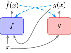
Figure 1: Co-training of classifier $f$ and adversarial generator. Solid arrows represent input/output relations; dashed arrows represent dependence of the loss function.

Concretely, our approach consists of co-training the classifier $f$, and a generator $g$ that maps inputs $x$ to approximate adversarial examples $g(x)$. Given a (current) classifier $f$, our loss function for $g$ for a training example $x$ is

$${\cal L}_{g}(x,\theta_{g})=\frac{1}{2}\|g(x;\theta_{g})-x\|^{2}+\max(\hat{f}(g(x;\theta_{G}))[i]-\hat{f}(g(x;\theta_{G}))[j],\ 0),$$ (9)

where $\theta_{g}$ are the trainable parameters of $g$, $i=f(x)$ is the label associated with $x$ by $f$, and $j\in{\cal Y}$ is the label with the second highest value in $\hat{f}(g(x;\theta_{G}))$. The first term of the loss function enforces that $g(x)$ is close to $x$. The second term is equal to zero if $f(g(x))\neq f(x)$, i.e., $g(x)$ is adversarial in the sense that it is labeled differently from $x$.

Given a (current) generator $g$, the classifier $f$ is trained using the following loss function for a labeled training example $(x,y)$:

$${\cal L}_{f}(x,\theta_{f})=-\log(\hat{f}(x)[y])+\lambda\frac{CE(\hat{f}(x),\hat{f}(g(x))}{1+\parallel x-g(x)\parallel^{2}}.$$ (10)

The first term here is the standard log loss. The second term is our robustness regularizer. It is essentially inversely proportional to how successful the generator $g$ is: the loss increases if $g$ finds close adversarial examples, i.e. $\parallel x-g(x)\parallel^{2}$ is small, and it increases when the output of $f$ at $g(x)$ is very different from the output of $f$ at $x$, as measured by $CE(\hat{f}(x),\hat{f}(g(x))$.

The models $f$ and $g$ are co-trained by an alternating stochastic gradient descent as shown in Algorithm 1.

Input: $D$, $f$, $g$, batchsize;

Randomly initialize $f$ and $g$;

while not converged do

       $\{I^{(f)}_{1},\ldots,I^{(f)}_{K}\}$ = shuffle(D) //create $K$ mini-batches according to batchsize;

       $\{I^{(g)}_{1},\ldots,I^{(g)}_{K}\}$ = shuffle(D);

       for $i=1$ to $K$ do

             $x^{\prime}_{j}=g(x_{j})\quad\forall\ j=1,\ldots,|I^{(f)}_{i}|$;

             Perform SGD update on $f$ using augmented mini-batch $\{x_{j},x^{\prime}_{j}\ |\ j=1,\ldots,|I_{i}^{(f)}|\}$;

             Perform SGD update on $g$ using inputs from $I_{i}^{(g)}$;

            

       end for

      

end while

Algorithm 1 Regularization Training for $R^{f}_{{\cal Q}_{[0,d]},{\mathbf{1}},p}$

3.2 Robustness Evaluation

Having learned a classifier $f$, we want to evaluate its $R^{f}_{{\cal Q}_{[0,d]},{\mathbf{1}},p}$ score. To obtain an empirical estimate based on a set of test points $x^{(i)}$, one would ideally determine precisely the classifier margin at each $x^{(i)}$. Since this is infeasible, we resort as usual to the distance between $x^{(i)}$ and an adversarial example for $x^{(i)}$ as an upper approximation of the margin. For this purpose we could re-use the generator model $g$ constructed in our robust training approach. However, this would lead to an unfair advantage of our models in comparsion to models learned using other robust training approaches. For scoring, we therefore construct adversarial examples $x^{*}$ using an ensemble approach, where we consider a set of state-of-the-art strategies for generating adversarial examples, FGSM [8], PGD [21], and BG [11]. Starting from a trained model $f$, for each $x$ in the test set, we construct the set $Adv(x)=\{x_{FGSM},x_{PDG},x_{BG}\}$, where its elements are generated according to the strategies mentioned above. Then, for each $x^{\prime}\in Adv(x)$ we consider $\hat{x}=x+\epsilon_{x^{\prime}}(x^{\prime}-x)$, where $\epsilon$ is the smallest positive real number such that $f(x+\epsilon(x^{\prime}-x))\neq f(x)\}$. In practise $\epsilon$ is estimated by a binary search under the assumption that there is only one decision boundary on the line between $x$ and $x^{\prime}$. Finally, we select from among $\hat{x}_{FGSM}$, $\hat{x}_{PDG}$, $\hat{x}_{BG}$ the one that lies closest to $x$ as the adversarial example $x^{*}$.

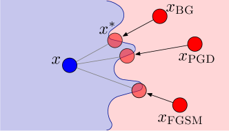
Figure 2: Ensemble approach for adversarial example construction. Shown are the decision boundary, a test point $x$, the adversarial examples generated for $x$ by the methods BG, PGD, FGSM, their associated points $\hat{x}$, and the finally selected $x^{*}$.

3.3 Experimental results

Figure 3: Qualitative and quantitative robustness results for the MNIST, CIFAR-10, SVHN, and F-MNIST. The legends report the area under the curves as quantitative measure of robustness. Higher areas corresponds to more robust models.

We evaluated the proposed training approach for Example 3 on 4 datasets: MNIST [19], CIFAR-10 [17], SVHN [23], and F(ashion)-MNIST [38]. MNIST contains $28\times 28$ pixel gray scale handwritten digits uniformly distributed over $10$ classes, divided in $60,000$ and $10,000$ examples for training and test respectively. SVHN contains $32\times 32$ pixel RGB images of street view house numbers uniformly distributed over $10$ classes, divided in $73,257$ and $26,032$ examples for training and test respectively. CIFAR-10 contains $32\times 32$ pixel RGB natural images uniformly distributed over $10$ classes, divided in $50,000$ and $10,000$ examples for training and test respectively. Finally F-MNIST is a dataset of Zalando’s article $28\times 28$ images, consisting of a training set of $60,000$ examples and a test set of $10,000$ examples, uniformly distributed within $10$ classes.

For each dataset we compared 3 neural networks $f$ which share the same structure: a model trained without any robustness regularization, a model trained with the regularization penalty from [11] , and a model trained according to our proposed regularization penalty defined in Equation 10, in conjunction with the adversarial generator described in Section 3.1.

For MNIST, SVHN, and F-MNIST we used for $f$ the same convolutional neural network architecture. For CIFAR-10, we used instead the state-of-the-art model ResNet 20 described in [10]. The generator $g$ is another convolutional neural network, whose structure is the same for all the datasets (with the exception of the filters of the last layer that depend whether the input picture is grayscale or RGB). The implementation details of $f$ and $g$ are described in the supplementary material. We first trained the models without any robustness regularization, obtaining accuracies as shown in the first column of Table 1. We then trained using the robustness regularizer of [11] (in the following referred to as Hein method) and our approach using different values of the $\lambda$ parameter that trades off accuracy vs. robustness (cf. Equation 10; Hein has a corresponding parameter). We report in the following the results that were obtained with the $\lambda$ parameter value that matched most closely the learning without robustness regularization in terms of test set accuracy. The second and third column of Table 1 show the obtained accuracies. Note that here we are not so much interested in improving the state of the art in terms of accuracy, but in improving robustness of reasonably accurate models. Therefore, we compare the robustness scores on models that have similar accuracies.

Table 1: Classification accuracies for the three setups for all the datasets.

Data set	No Reg.	Hein	Ours
MNIST	99.42%	99.12%	99.49%
CIFAR-10	91.15%	90.61%	90.38%
SVHN	92.64%	92.08%	92.33%
F-MINST	93.47%	92.80%	93.57%

For evaluating the robustness of the models, we used the adversarial example construction described in Section 3.2. In Figure 3 we plot the $R^{f}_{Q_{\epsilon},{\mathbf{1}},p}$ scores against $\epsilon$-values. These are essentially the marginal curves defined by [9]. The areas under these curves, i.e. our $R^{f}_{{\cal Q}_{[0,d]},{\mathbf{1}},p}$ score are reported in the legends, denoted with $R$. The results suggest that our proposed method allows to learn more robust models while keeping the accuracy almost unchanged. We also evaluated the effectiveness of the three methods BG, FGSM and PGD for generating adversarial examples. Due to the space limitation this analysis is reported in the supplementary material.

4 Unknown, large distribution shifts

In contrast to the adversarial robustness considered in the previous section, robustness under distribution shift or common corruptions [27] addresses the situation where new test cases may differ substantially from the original training data, which in our framework means that the conditional distribution $Q(\cdot|x)$ is not concentrated in an $\epsilon$-neighborhood of $x$. Without such a locality assumption on $Q$, it is then very difficult to encapsulate a sufficiently general robustness requirement by the specification of a specific family ${\cal Q}$ in analogy to ${\cal Q}_{[0,d]}$ of the previous section.

Recent investigations on distribution shift robustness are mostly based on image benchmark datasets, where an existing collection of labeled images is extended with additional test sets consisting of original test images that are modified by different types of corruptions, such as blurring, rotations, or change in brightness. Corrupted test sets of this kind have been introduced for the MNIST character recognition set [22], and for ImageNet [12]. The goal then is to train a model on original, uncorrupted, training data, such that it maintains high accuracy on the corrupted test images. Trying to obtain robustness in this setting by robust training techniques developed for adversarial robustness has met with limited success [22, 27]. Current state-of-the-art approaches for corruption robustness are based on training set augmentation, where additional training instances are generated from a mixture of pre-defined image perturbations [13], or added Gaussian noise sampled from a noise distribution optimized by co-training the classifier and the noise generator [27].

Most existing approaches are quite tightly linked to image data and neural network classifiers. We propose a general method that is not based on any specific properties of image data, and that can be combined with any type of classifier. Seeing that in this context a preservation of accuracy is the goal (not resistance to adversarial attacks), we are aiming for robustness as measured by $R^{f}_{Q,{\mathit{i}d},p}$ (cf. Proposition 6). However, the transition kernel $Q$ modeling the shift in the data distribution is not known a-priori. Our general idea is to

1.

learn a classifier $f$ from labeled training examples $(x,y)$ sampled from $P(X)P(Y|X)$;

2.

from original data points $x$, and new unlabeled examples $\tilde{x}$ sampled from $Q\circ P$, learn a transfer mapping $T$ that approximates an inversion of the transition $x\mapsto\tilde{x}\sim Q(|x)$;

3.

classify new test instances $\tilde{x}$ as $f(T(\tilde{x}))$.

The learning of $f$ and $T$ are completely separate, which allows the method to be used in conjunction with any type of classifier. Since in step 2. we are using examples from $Q\circ P$, this approach does not follow the strict condition that all training has to be done on the original, uncorrupted training set. However, the approach reflects a realistic application scenario, where one modifies an original classifier $f$ to a classifier $f\circ T$ adapted to a changing data distribution. It is important to note that for this adaptation we neither require labeled examples $(\tilde{x},y)$, nor do we use supervision in the form of given pairs $(x,\tilde{x})$ for which $\tilde{x}\sim Q(\cdot|x)$. In effect, our approach can be seen as a type of transductive transfer learning in the sense of [25].

Our approach for constructing a transfer model $T$ follows a paired auto-encoder architecture that in similar form has previously been used for the quite different application of deep fake generation [24]. We jointly train a pair of autoencoders to reconstruct samples of original points $x$, and corrupted points $\tilde{x}$. The two autoencoderes share the same encoder $E$, but have different decoders, $D_{1}$ and $D_{2}$, as depicted in Figure 4 (left) for the case of clean and corrupted MNIST digits. The transfer function $T$ then is defined as $T(\tilde{x})=D_{1}(E(\tilde{x}))$ (see Figure 4 (right)).

Table 2: Classification accuracies for NN and SVM models using different robust robust training techniques. For both models, the first row reprents the average accuracy over the 15 different corruption types. The second row shows the accuracy on the original MNIST test set. The standard deviation are estimated by training the models (including the autoencoders) with 5 different weight initializations.

Model	Plain	Gauss	Transfer-Separate				Transfer-Joint
			0	128	1024	30k	128	1024	30k
NN	86.3$\pm$0.52	88.5$\pm$0.38	86.4$\pm$0.87	88.5$\pm$0.44	91.1$\pm$0.16	92.8$\pm$0.09	88.5$\pm$0.17	91.5$\pm$0.05	92.1$\pm$0.15
	99.1$\pm$0.03	99.3$\pm$0.05	99.1$\pm$0.03	99.0$\pm$0.02	99.0$\pm$0.04	99.1$\pm$0.01	99.0$\pm$0.01	99.1$\pm$0.05	99.1$\pm$0.01
SVM	69.7	70.6$\pm$0.07	70.7$\pm$0.74	81.0$\pm$0.89	86.2$\pm$0.41	87.8$\pm$0.30	83.1$\pm$0.67	85.4$\pm$0.41	85.4$\pm$0.40
	98.4	97.9$\pm$0.02	98.3$\pm$0.06	98.3$\pm$0.06	98.2$\pm$0.02	98.3$\pm$0.03	98.2$\pm$0.07	98.3$\pm$0.05	98.3$\pm$0.03

We evaluate our method using the C-MNIST [22] suite of 15 corruptions applied to the MNIST training and test sets. We consider two different classifers: a Neural Network (NN), and a support vector machine (SVM) with RBF kernel. For the NN we used the same architecture as used by [22]. The details regarding the structure and the training of $f$, $E$, $D_{1}$, and $D_{2}$ are reported in the supplementary material. We use two different evaluation setups:

• Transfer-Separate: we train and test transfer models with data of one of the 15 corruption types at a time. Hence, in total we construct 15 different pairs of autoencoders. Corrupted test images are classified using the transfer model learned from examples of the corresponding corruption type.

• Transfer-Joint: for training, we pool all the 15 corruption types into one set for training a single pair of autoencoders. Test images with all corruption types are classified using the same resulting transfer model.

For both Transfer-Separate and Transfer-Joint we use for training $N_{o}=60k-15N_{c}$ examples $x$ from the original MNIST dataset and $N_{c}\in\{0,128,1024,30k\}$ examples $\tilde{x}$ for each of the 15 corruption classes from the C-MNIST training set. We ensure that none of the $\tilde{x}$ used for training is the corrupted version of a clean $x$ also used for training. The case $N_{c}=0$, means that we only train one autoencoder consisting of $E$, and $D_{1}$ which then still can be used as a transfer model for new, corrupted examples. There is no difference between Transfer-Joint and Transfer-Separate in this case.

Figure 4: Transfer by paired auto-encoders

As baselines we consider Plain classifiers wich are obtained by standard training on clean images, and then used without modifications to classify noisy images. As a second baseline we used data augmentation by adding Gaussian noise to the original MNIST pictures. The Gaussian noise centered in 0 with standard deviation of 0.1, was applied independently for each pixel. NN and SVM classifiers were then learned from a mix of clean and noisy examples.

Table 2 shows a summary of results. For each classifer we report the accuracy on corrupted test images, averaged over the 15 corruption types, and the accuracy for the original MNIST test set We first observe that adding a robust training approach nowhere leads to a significant decrease in the clean data accuracy. Both the Plain NN and SVM models are significantly less accuracte on the noisy than the clean data, where the gap is even more pronounced for SVM than NN. The Gauss baseline for robust training in this experiment only led to a minor improvement. This is in contrast to findings by [27], who reported that Gaussian noise augmentation can be quite effective. However, they also show that a very careful calibration of the Gaussian noise generation is required. The results for both Transfer approaches show a significant improvement of classification accuracy for the corrupted examples as the number of noisy training examples increases. This improvement is consistent for the NN and SVM models. Most remarkably, perhaps, the results for Transfer-Separate and Transfer-Joint are very similar, showing that a single transfer model $T$ can handle a wide range of different data transformations.

[22] reported an accuracy of $91.91\%$ for what should correspond exactly to our Plain NN model. We were unable to reproduce their results, and only obtained the $86.30\%\pm 0.52$ shown in the table. [27] report and accuracy of $92.2\%$ for their trained Gaussian noise augmentation approach. However, these results are not directly comparable, since [27] use a different neural network architecture.

5 Conclusions

We have introduced a general framework for defining robustness of classifiers. Our framework allows flexible definitions for different types of robustness that in a uniform manner permit to calibrate robustness objectives with respect to different assumptions on the nature of adversarial attacks or distribution changes that one wants to protect against. Our framework establishes a natural link between the recent work in robustness, and more established work in the area of transfer learning. Considering two specific robustness concepts, we have developed new training methods for image classifiers for these robustness objectives. Our results show particularly promising results in a learning setting where a classifier can be incrementally trained to become more robust by being exposed to novel, unlabeled examples.

While being greatly motivated by the conceptual framework, our algorithmic solutions are not directly linked to the formal foundations we laid in this paper. A possible line of future work can be the development of more generic training methods that can then be simply instantiated for a given robustness objectives. On the theoretical side, an interesting question would be to what extent robustness for a given measure $R_{Q,H,G}$ implies lower bounds on the robustness according to another measure $R_{Q^{\prime},H^{\prime},G^{\prime}}$, and, thus, whether one type of robustness as a training objective typically leads to models that are robust in a wider sense.

Supplementary Material

Appendix A Details for Section 3.3

A.1 Model architectures used in the experiments

For the experiments, we chose a relatively simple convolutional neural network, which is considered the state-of-the-art method for image classification (see, e.g., [33]), and it can still provide reasonable high accuracies. The convolutional neural network $f$ architecture used for MNIST [19], SVHN [23], and F(ashion)-MNIST [38] is depicted in Figure 5. $N=28$, $C=1$ for F-MNIST and MNIST, while $N=32$, $C=3$ for SVHN. Each convolutional layer ($5\times 5$ kernels; stride 1; 128 channels), is followed by batch normalization [14] and LeakyReLU [20] activations ($\alpha=0.1$). The two dense layers has $1024$ and $10$ units respectively. The first is followed by batch normalization and LeakyReLU activations; the second is followed by softmax activations). For CIFAR-10 [17] we used for $f$ the ResNet20 architecture described in [10].

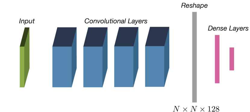
Figure 5: Architecture of $f$ used for F-MNIST, MNIST, and SVHN.

$g$ is another convolutional neural network, whose structure, depicted in Figure 6, is the same for all the datasets (with the exception of the filters of the last layer that depend whether the input picture is grayscale or RGB). $N=28$, $C=1$ for F-MNIST and MNIST, while $N=32$, $C=3$ for SVHN and CIFAR-10. Here again each intermediate convolutional layer ($5\times 5$ kernels; stride 1; 128 channels), is followed by batch normalization and LeakyReLU activations ($\alpha=0.1$). The output layer is another convolutional layer with sigmoid activations.

Figure 6: Architecture of $g$ used for F-MNIST, MNIST, SVHN. and CIFAR-10.

For each dataset we reserved $10\%$ of examples as validation set. During the training, we then selected the best model based on the accuracy on the validation set. For F-MNIST, MNIST and SVHN. The weights of $f$ and $g$ are updated with Adam [15] optimizer on mini-batches of size 32 for 10 epochs. For both $f$ and $g$ the learning rates are set to $0.001$ for the first 5 epochs , and $1\mathrm{e}{-4}$ after. For CIFAR-10 the weights of $f$ and $g$ are updated with Adam optimizer on mini-batches of size 32 for 200 epochs. The learning rates are set to $0.001$ for the first 80 epochs, $1\mathrm{e}{-4}$ until the 120th epoch, $1\mathrm{e}{-5}$ until the 160th epoch, and finally $0.5\mathrm{e}{-6}$ after. We used the MNIST dataset contained in the tensorflow library (https://www.tensorflow.org) and the F-MNIST dataset downloadable from https://github.com/zalandoresearch/fashion-mnist.

A.2 Additional results

Table 3: For each method and dataset, the columns represent the percentage of closest adversarial examples to the original examples, after the binary search.

Dataset	No Reg			Hein			Ours
	BG	FGSM	PGD	BG	FGSM	PGD	BG	FGSM	PGD
MNIST	97.84	0.58	1.58	71.92	0.88	27.20	13.68	0.52	85.80
CIFAR-10	99.78	0.00	0.22	99.96	0.00	0.04	98.77	0.00	1.23
SVHN	93.53	6.38	0.09	92.78	7.21	0.01	92.78	7.21	0.01
F-MNIST	93.17	6.18	0.65	92.46	7.03	0.51	82.43	6.28	11.29

Table 3 reports the percentage of training examples for which the respective methods led to the final closest adversarial example $x^{*}$ (for each dataset and for each method). The results suggest that the BG technique produces in general closer adversarial examples to the original inputs. It is worth pointing out that this shows that the results reported in Figure 3 are mostly based on adversarial examples generated by the BG method, which the Hein method is designed to defend against.

Examples of adversarial examples generated with the BG algorithm and their $L_{2}$-distance to the original data point are depicted in Figure 7. This illustrates that the adversarial example for our method is visually significantly more distinct than the adversarial examples for the other two methods. A larger and systematic set of illustrative examples is given in the supplementary material.

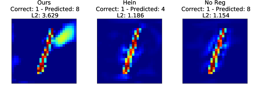
Figure 7: Examples of adversarial examples closed to the margin generated by using  [11] for the three models. The three adversarial examples are generated according to the same input picture. From left to right, the adversarial examples are constructed from the models with the proposed regularization, the regularization proposed by [11], and no regularization.

Appendix B Details for Experiments of Section 4

Layer notation:

• Conv2D($c$, $k$, $s$, $a$) / Conv2DTranspose($c$, $k$, $s$, $a$), where $c$ is the number of filters, $k$ is the kernel size, $s$ is the stride, and $a$ is the activation function;

• MaxPooling($s$), where $s$ is the stride;

• Dense($u$,$a$), where $u$ represents the number of units, and $a$ the activation function;

• Dropout($r$), where $r$ represents the rate;

The Neural Network classifer has the following structure:

$$\text{Conv2D(32, 3, 1, `relu')}\rightarrow\text{Conv2D(64, 3, 1,`relu')}\rightarrow$$

$$\text{MaxPooling(2)}\rightarrow\text{Dropout(0.25)}\rightarrow\text{Flatten()}\rightarrow$$

$$\text{Dense(128, `relu')}\rightarrow\text{Dropout(0.5)}\rightarrow$$

Dense(10, ‘softmax’)

We reserved $10\%$ of examples as validation set. During the training, we then selected the best model based on the accuracy on the validation set. The weights of the model are updated with Adam [15] optimizer on mini-batches of size 32 for 50 epochs. The learning rate is set to $0.001$.

SVM uses the RBF kernel with $\gamma=0.05$ and $C=5$.

The architecture for $E$ is the following:

$$\text{Conv2D(32, 3, 2, `relu')}\rightarrow\text{Conv2D(64, 3, 2,`relu')}\rightarrow$$

$$\text{Conv2D(128, 3, 2, `relu')}\rightarrow\text{Flatten()}\rightarrow$$

Dense(128, ‘linear’)

$D_{1}$ and $D_{2}$ share the following architecture:

$$\text{Dense(2048, `relu')}\rightarrow\text{Dense(7*7*64, `relu')}\rightarrow$$

$$\text{Reshape((7,7,64))}\rightarrow$$

$$\text{Conv2DTranspose(64, 3, 2, `relu')}\rightarrow$$

$$\text{Conv2DTranspose(32, 3, 2, `relu')}\rightarrow$$

$$\text{Conv2DTranspose(1, 3, 1, `sigmoid')}\rightarrow$$

$E$, $D_{1}$, and $D_{2}$ are jointly trained minimizing the reconstruction loss for 100 epochs. We used Adam with learning rate equals to $1e-3$ and batch size 32.

Table 4: Classification accuracies for all the corruptions of C-MNIST datasets for the neural network model.

Model	Plain	Gauss	Transfer-Separate				Transfer-Joint
			0	128	1024	30k	128	1024	30k
brightness	98.8$\pm$0.02	75.1$\pm$0.52	98.8$\pm$0.02	98.6$\pm$0.03	98.6$\pm$0.03	98.9$\pm$0.04	98.7$\pm$0.05	98.9$\pm$0.05	98.9$\pm$0.01
canny edges	81.2$\pm$0.46	79.9$\pm$0.53	81.5$\pm$0.46	81.1$\pm$0.63	81.7$\pm$0.64	81.8$\pm$0.54	81.5$\pm$0.32	81.8$\pm$0.20	81.5$\pm$0.20
dotted line	97.2$\pm$0.52	98.3$\pm$0.39	97.0$\pm$0.52	97.3$\pm$0.31	97.4$\pm$0.23	98.4$\pm$0.08	93.4$\pm$0.51	95.3$\pm$0.38	98.7$\pm$0.22
fog	93.9$\pm$0.60	64.6$\pm$0.44	93.9$\pm$1.00	93.0$\pm$0.72	97.3$\pm$0.21	98.9$\pm$0.02	86.4$\pm$1.48	95.2$\pm$0.43	95.3$\pm$0.66
glass blur	89.7$\pm$0.48	92.8$\pm$0.42	89.8$\pm$0.56	92.2$\pm$1.48	93.9$\pm$0.22	93.4$\pm$0.56	92.9$\pm$0.08	92.6$\pm$0.30	92.3$\pm$0.24
identity	99.1$\pm$0.03	99.3$\pm$0.71	99.1$\pm$0.03	99.0$\pm$0.02	99.0$\pm$0.04	99.1$\pm$0.01	99.0$\pm$0.01	99.1$\pm$0.05	99.1$\pm$0.01
impulse noise	88.6$\pm$0.78	93.4$\pm$0.58	88.8$\pm$1.12	84.7$\pm$2.04	90.4$\pm$0.31	93.8$\pm$0.68	71.4$\pm$0.33	92.4$\pm$0.27	93.4$\pm$0.22
motion blur	84.7$\pm$1.41	95.8$\pm$0.14	84.6$\pm$2.11	82.3$\pm$1.01	91.2$\pm$0.55	96.0$\pm$0.28	91.9$\pm$0.41	93.8$\pm$0.26	93.2$\pm$0.32
rotate	90.7$\pm$0.10	92.1$\pm$0.24	90.7$\pm$0.10	90.1$\pm$0.07	91.1$\pm$0.41	91.9$\pm$0.09	90.5$\pm$0.13	91.0$\pm$0.04	92.1$\pm$0.07
scale	91.5$\pm$0.23	94.3$\pm$0.33	91.5$\pm$0.29	87.4$\pm$0.87	87.6$\pm$0.33	94.4$\pm$0.18	90.9$\pm$0.47	92.7$\pm$0.21	94.1$\pm$0.11
shear	97.1$\pm$0.09	98.0$\pm$0.50	97.1$\pm$0.11	95.6$\pm$0.17	96.3$\pm$1.44	96.9$\pm$0.08	96.8$\pm$0.08	97.4$\pm$0.07	97.5$\pm$0.07
shot noise	97.6$\pm$0.12	97.7$\pm$0.33	97.6$\pm$0.08	91.6$\pm$3.34	97.3$\pm$0.31	97.3$\pm$0.07	97.7$\pm$0.10	97.8$\pm$0.08	97.8$\pm$0.10
spatter	96.8$\pm$0.06	98.4$\pm$0.40	96.8$\pm$0.08	94.7$\pm$1.38	95.1$\pm$0.20	97.2$\pm$0.09	96.8$\pm$0.16	96.9$\pm$0.07	96.9$\pm$0.10
stripe	33.8$\pm$4.50	95.6$\pm$0.11	33.3$\pm$7.50	78.1$\pm$1.21	90.8$\pm$0.44	93.5$\pm$0.46	85.2$\pm$2.19	93.6$\pm$0.55	93.9$\pm$0.42
translate	52.6$\pm$0.12	51.8$\pm$0.16	52.5$\pm$0.20	56.8$\pm$1.19	56.5$\pm$0.27	56.3$\pm$0.27	56.2$\pm$0.17	56.8$\pm$0.06	53.1$\pm$0.04
zigzag	87.6$\pm$0.32	89.5$\pm$0.37	87.6$\pm$0.38	92.9$\pm$0.42	92.7$\pm$0.31	96.2$\pm$0.23	86.8$\pm$0.48	88.4$\pm$0.28	95.5$\pm$0.20

Table 5: Classification accuracies for all the corruptions of C-MNIST datasets for the SVM model.

Model	Plain	Gauss	Transfer-Separate				Transfer-Joint
			0	128	1024	30k	128	1024	30k
brightness	69.7	97.7$\pm$0.02	98.1$\pm$0.09	98.0$\pm$0.03	97.9$\pm$0.07	98.2$\pm$0.03	98.1$\pm$0.04	98.1$\pm$0.02	98.1$\pm$0.06
canny edges	69.7	34.4$\pm$0.05	60.4$\pm$1.12	44.3$\pm$1.82	72.5$\pm$1.03	70.3$\pm$1.14	58.5$\pm$1.13	62.7$\pm$1.49	61.5$\pm$1.18
dotted line	69.7	97.0$\pm$0.02	97.2$\pm$0.22	94.1$\pm$0.54	95.2$\pm$0.50	98.0$\pm$0.08	95.5$\pm$0.27	96.1$\pm$0.39	96.5$\pm$0.23
fog	69.7	58.8$\pm$0.12	94.2$\pm$0.94	92.4$\pm$0.65	96.8$\pm$0.18	98.2$\pm$0.04	84.6$\pm$1.56	91.6$\pm$1.00	91.1$\pm$0.86
glass blur	69.7	93.8$\pm$0.06	90.7$\pm$1.03	94.0$\pm$2.35	95.0$\pm$0.32	96.2$\pm$0.15	94.7$\pm$0.34	95.6$\pm$0.19	95.5$\pm$0.19
identity	69.7	97.9$\pm$0.02	98.3$\pm$0.06	98.3$\pm$0.06	98.2$\pm$0.02	98.3$\pm$0.03	98.2$\pm$0.07	98.3$\pm$0.05	98.3$\pm$0.03
impulse noise	69.7	25.4$\pm$0.04	92.6$\pm$0.52	63.7$\pm$3.42	89.3$\pm$0.75	94.0$\pm$0.64	73.9$\pm$2.52	91.9$\pm$0.34	93.4$\pm$0.65
motion blur	69.7	85.8$\pm$0.11	84.7$\pm$0.77	83.0$\pm$0.65	89.3$\pm$0.40	93.4$\pm$0.45	87.3$\pm$0.34	88.0$\pm$0.57	88.1$\pm$0.70
rotate	69.7	86.9$\pm$0.02	88.2$\pm$0.13	87.7$\pm$0.03	87.3$\pm$0.20	88.2$\pm$0.06	88.1$\pm$0.12	88.5$\pm$0.08	88.5$\pm$0.12
scale	69.7	51.1$\pm$0.39	64.1$\pm$0.75	63.5$\pm$0.78	65.2$\pm$1.26	67.6$\pm$1.09	63.7$\pm$1.03	64.4$\pm$0.92	64.0$\pm$0.84
shear	69.7	93.8$\pm$0.02	94.8$\pm$0.13	93.3$\pm$0.16	92.4$\pm$0.19	94.5$\pm$0.15	94.7$\pm$0.12	95.0$\pm$0.08	95.0$\pm$0.07
shot noise	69.7	97.1$\pm$0.06	97.1$\pm$0.18	95.4$\pm$1.20	96.6$\pm$0.24	97.7$\pm$0.06	97.2$\pm$0.13	97.5$\pm$0.11	97.5$\pm$0.07
spatter	69.7	96.7$\pm$0.04	96.1$\pm$0.28	94.7$\pm$1.21	95.3$\pm$0.22	96.9$\pm$0.04	96.6$\pm$0.11	96.8$\pm$0.08	96.7$\pm$0.07
stripe	69.7	10.3$\pm$0.00	22.4$\pm$4.71	77.9$\pm$0.83	92.1$\pm$0.41	94.5$\pm$0.59	88.4$\pm$1.64	94.6$\pm$0.66	94.8$\pm$0.45
translate	69.7	21.6$\pm$0.05	23.5$\pm$0.15	22.5$\pm$0.31	21.3$\pm$0.30	21.0$\pm$0.18	23.3$\pm$0.10	23.2$\pm$0.13	22.9$\pm$0.22
zigzag	69.7	80.8$\pm$0.12	89.1$\pm$0.78	93.3$\pm$0.26	94.2$\pm$0.46	97.2$\pm$0.11	87.5$\pm$1.12	84.8$\pm$0.52	84.2$\pm$0.68

References

- Bunel et al. [2017] Rudy Bunel, Ilker Turkaslan, Philip H. S. Torr, Pushmeet Kohli, and M. Pawan Kumar. Piecewise linear neural network verification: A comparative study. CoRR, abs/1711.00455, 2017. URL http://arxiv.org/abs/1711.00455.
- Cisse et al. [2017] Moustapha Cisse, Piotr Bojanowski, Edouard Grave, Yann Dauphin, and Nicolas Usunier. Parseval networks: Improving robustness to adversarial examples. In Doina Precup and Yee Whye Teh, editors, Proceedings of the 34th International Conference on Machine Learning, volume 70 of Proceedings of Machine Learning Research, pages 854–863, International Convention Centre, Sydney, Australia, 06–11 Aug 2017. PMLR. URL http://proceedings.mlr.press/v70/cisse17a.html.
- Dvijotham et al. [2018] Krishnamurthy Dvijotham, Robert Stanforth, Sven Gowal, Timothy Mann, and Pushmeet Kohli. A dual approach to scalable verification of deep networks. arXiv preprint arXiv:1803.06567, 2018.
- Ehlers [2017] Ruediger Ehlers. Formal verification of piece-wise linear feed-forward neural networks. In International Symposium on Automated Technology for Verification and Analysis, pages 269–286. Springer, 2017.
- Elsayed et al. [2018] Gamaleldin Elsayed, Dilip Krishnan, Hossein Mobahi, Kevin Regan, and Samy Bengio. Large margin deep networks for classification. In Advances in neural information processing systems, pages 842–852, 2018.
- Ford et al. [2019] Nicolas Ford, Justin Gilmer, Nicholas Carlini, and Ekin D. Cubuk. Adversarial examples are a natural consequence of test error in noise. In International Conference on Machine Learning, pages 2280–2289. PMLR, 2019.
- Fukushima [1980] Kunihiko Fukushima. Neocognitron: A self-organizing neural network model for a mechanism of pattern recognition unaffected by shift in position. Biological cybernetics, 36(4):193–202, 1980.
- Goodfellow et al. [2014] Ian J Goodfellow, Jonathon Shlens, and Christian Szegedy. Explaining and harnessing adversarial examples. arXiv preprint arXiv:1412.6572, 2014.
- Göpfert et al. [2019] Christina Göpfert, Jan Philip Göpfert, and Barbara Hammer. Adversarial robustness curves. arXiv preprint arXiv:1908.00096, 2019.
- He et al. [2016] Kaiming He, Xiangyu Zhang, Shaoqing Ren, and Jian Sun. Deep residual learning for image recognition. In Proceedings of the IEEE conference on computer vision and pattern recognition, pages 770–778, 2016.
- Hein and Andriushchenko [2017] Matthias Hein and Maksym Andriushchenko. Formal guarantees on the robustness of a classifier against adversarial manipulation. In Advances in Neural Information Processing Systems, pages 2266–2276, 2017.
- Hendrycks and Dietterich [2018] Dan Hendrycks and Thomas Dietterich. Benchmarking neural network robustness to common corruptions and perturbations. In International Conference on Learning Representations, 2018.
- Hendrycks et al. [2019] Dan Hendrycks, Norman Mu, Ekin Dogus Cubuk, Barret Zoph, Justin Gilmer, and Balaji Lakshminarayanan. Augmix: A simple data processing method to improve robustness and uncertainty. In International Conference on Learning Representations, 2019.
- Ioffe and Szegedy [2015] Sergey Ioffe and Christian Szegedy. Batch normalization: Accelerating deep network training by reducing internal covariate shift. arXiv preprint arXiv:1502.03167, 2015.
- Kingma and Ba [2014] Diederik P Kingma and Jimmy Ba. Adam: A method for stochastic optimization. arXiv preprint arXiv:1412.6980, 2014.
- Kolesnikov et al. [2019] Alexander Kolesnikov, Lucas Beyer, Xiaohua Zhai, Joan Puigcerver, Jessica Yung, Sylvain Gelly, and Neil Houlsby. Large scale learning of general visual representations for transfer. arXiv preprint arXiv:1912.11370, 2019.
- Krizhevsky et al. [2009] Alex Krizhevsky, Geoffrey Hinton, et al. Learning multiple layers of features from tiny images. Technical report, Citeseer, 2009.
- LeCun et al. [1989] Yann LeCun, Bernhard Boser, John S Denker, Donnie Henderson, Richard E Howard, Wayne Hubbard, and Lawrence D Jackel. Backpropagation applied to handwritten zip code recognition. Neural computation, 1(4):541–551, 1989.
- LeCun et al. [1998] Yann LeCun, Léon Bottou, Yoshua Bengio, Patrick Haffner, et al. Gradient-based learning applied to document recognition. Proceedings of the IEEE, 86(11):2278–2324, 1998.
- Maas et al. [2013] Andrew L Maas, Awni Y Hannun, and Andrew Y Ng. Rectifier nonlinearities improve neural network acoustic models. In Proc. icml, volume 30, page 3, 2013.
- Madry et al. [2018] Aleksander Madry, Aleksandar Makelov, Ludwig Schmidt, Dimitris Tsipras, and Adrian Vladu. Towards deep learning models resistant to adversarial attacks. In 6th International Conference on Learning Representations, ICLR 2018, Vancouver, BC, Canada, April 30 - May 3, 2018, Conference Track Proceedings. OpenReview.net, 2018. URL https://openreview.net/forum?id=rJzIBfZAb.
- Mu and Gilmer [2019] Norman Mu and Justin Gilmer. Mnist-c: A robustness benchmark for computer vision. arXiv preprint arXiv:1906.02337, 2019.
- Netzer et al. [2011] Yuval Netzer, Tao Wang, Adam Coates, Alessandro Bissacco, Bo Wu, and Andrew Y Ng. Reading digits in natural images with unsupervised feature learning. In Advances in Neural Information Processing Systems, 2011.
- Nguyen et al. [2019] Thanh Thi Nguyen, Cuong M. Nguyen, Dung Tien Nguyen, Duc Thanh Nguyen, and Saeid Nahavandi. Deep learning for deepfakes creation and detection. CoRR, abs/1909.11573, 2019. URL http://arxiv.org/abs/1909.11573.
- Pan and Yang [2009] Sinno Jialin Pan and Qiang Yang. A survey on transfer learning. IEEE Transactions on knowledge and data engineering, 22(10):1345–1359, 2009.
- Ruan et al. [2018] Wenjie Ruan, Xiaowei Huang, and Marta Kwiatkowska. Reachability analysis of deep neural networks with provable guarantees. In Proceedings of the 27th International Joint Conference on Artificial Intelligence, pages 2651–2659. AAAI Press, 2018.
- Rusak et al. [2020] Evgenia Rusak, Lukas Schott, Roland S Zimmermann, Julian Bitterwolf, Oliver Bringmann, Matthias Bethge, and Wieland Brendel. A simple way to make neural networks robust against diverse image corruptions. In European Conference on Computer Vision, pages 53–69. Springer, 2020.
- Sinha et al. [2019] Abhishek Sinha, Mayank Singh, Nupur Kumari, Balaji Krishnamurthy, Harshitha Machiraju, and VN Balasubramanian. Harnessing the vulnerability of latent layers in adversarially trained models. arXiv preprint arXiv:1905.05186, 2019.
- Stutz et al. [2019] David Stutz, Matthias Hein, and Bernt Schiele. Disentangling adversarial robustness and generalization. In Proceedings of the IEEE Conference on Computer Vision and Pattern Recognition, pages 6976–6987, 2019.
- Su et al. [2018] Dong Su, Huan Zhang, Hongge Chen, Jinfeng Yi, Pin-Yu Chen, and Yupeng Gao. Is robustness the cost of accuracy?–a comprehensive study on the robustness of 18 deep image classification models. In Proceedings of the European Conference on Computer Vision (ECCV), pages 631–648, 2018.
- Su et al. [2019] Jiawei Su, Danilo Vasconcellos Vargas, and Kouichi Sakurai. One pixel attack for fooling deep neural networks. IEEE Transactions on Evolutionary Computation, 2019.
- Szegedy et al. [2013] Christian Szegedy, Wojciech Zaremba, Ilya Sutskever, Joan Bruna, Dumitru Erhan, Ian Goodfellow, and Rob Fergus. Intriguing properties of neural networks. arXiv preprint arXiv:1312.6199, 2013.
- Szegedy et al. [2017] Christian Szegedy, Sergey Ioffe, Vincent Vanhoucke, and Alexander A Alemi. Inception-v4, inception-resnet and the impact of residual connections on learning. In Thirty-First AAAI Conference on Artificial Intelligence, 2017.
- Tramèr and Boneh [2019] Florian Tramèr and Dan Boneh. Adversarial training and robustness for multiple perturbations. In 2019 Conference on Neural Information Processing Systems (NeurIPS), volume 32, 2019.
- Tsipras et al. [2018] Dimitris Tsipras, Shibani Santurkar, Logan Engstrom, Alexander Turner, and Aleksander Madry. Robustness may be at odds with accuracy. arXiv preprint arXiv:1805.12152, 2018.
- Weng et al. [2018] Tsui-Wei Weng, Huan Zhang, Pin-Yu Chen, Jinfeng Yi, Dong Su, Yupeng Gao, Cho-Jui Hsieh, and Luca Daniel. Evaluating the robustness of neural networks: An extreme value theory approach. In International Conference on Learning Representations, 2018.
- Wicker et al. [2020] Matthew Wicker, Luca Laurenti, Andrea Patane, and Marta Kwiatkowska. Probabilistic safety for bayesian neural networks. In Conference on Uncertainty in Artificial Intelligence, pages 1198–1207. PMLR, 2020.
- Xiao et al. [2017] Han Xiao, Kashif Rasul, and Roland Vollgraf. Fashion-mnist: a novel image dataset for benchmarking machine learning algorithms. arXiv preprint arXiv:1708.07747, 2017.
- Xie et al. [2019] Qizhe Xie, Eduard Hovy, Minh-Thang Luong, and Quoc V Le. Self-training with noisy student improves imagenet classification. arXiv preprint arXiv:1911.04252, 2019.