Controlling the quantum speed limit time for unital maps via filtering operations

Abstract

The minimum time a system needs to change from an initial state to a final orthogonal state is called quantum speed limit time. Quantum speed limit time can be used to quantify the speed of the quantum evolution. The speed of the quantum evolution will increase, if the quantum speed limit time decreases. In this work we will use relative purity based bound for quantum speed limit time. It is applicable for any arbitrary initial state. Here, we investigate the effects of filtering operation on quantum speed limit time. It will be observed that for some intervals of filtering operation parameter the quantum speed limit time is decreased by increasing filtering operation parameter and for some other intervals it is decreased by decreasing filtering operation parameter.

I Introduction

The dynamical speed of a quantum evolution is one of the most important concepts in quantum theory. It also has wide applications in quantum theory, such as quantum communication Duan ; Bekenstein , quantum metrology Giovannetti1 ; Giovannetti2 , optimal control Caneva and etc. Quantum theory sets a bound on speed of the evolution of quantum systems. The minimal time it takes for the quantum system to transform from an initial state to a target state is known as quantum speed limit (QSL) time. QSL time determines the maximum speed of dynamical evolution. There have been many attempts to introduce a comprehensive bound for QSL time. In Ref.Mandelstam , Mandelstam and Tamm have introduced a bound for QSL time in closed quantum systems, which reads

$$\tau\geq\tau_{QSL}=\frac{\pi\hbar}{2\Delta E},$$ (1)

where $\Delta E=\sqrt{\langle\hat{H}^{2}\rangle-\langle\hat{H}\rangle^{2}}$ is the variation of energy of the initial state and $\hat{H}$ is time-independent Hamiltonian describing the dynamics of quantum system. This bound is called MT bound. In Ref.Margolus , Margolus and Levitin have introduced the bound for closed quantum system based on the mean energy $E=\langle\hat{H}\rangle$ as

$$\tau\geq\tau_{QSL}=\frac{\pi\hbar}{2E},$$ (2)

this bound is called ML bound. Using these two bounds one can obtain a comprehensive bound as followsGiovannetti3

$$\tau\geq\tau_{QSL}=\max\left\{\frac{\pi\hbar}{2\Delta E},\frac{\pi\hbar}{2E}\right\}$$ (3)

In Refs.Jones ; Deffner ; Pfeifer ; Pfeifer1 ,the generalizations of the MT and ML bounds to nonorthogonal states and to driven systems have been determines. The QSL time for the dynamics of open systems is also investigated in Refs. Taddei ; delCampo ; Deffner1 . An unified bound of QSL time including both MT and ML types for non- Markovian dynamics has formulated in Ref. Deffner1 . However this bound is used for initial pure state and it is not feasible for mixed initial states. In Ref.zhang , the authors introduce the bound for QSL time which can be used for arbitrary initial states. They obtained a QSL time for mixed initial states by introducing relative purity as the distance measure, which can define the speed of evolution starting from an arbitrary initial state in the dynamics of open quantum systems.

QSL time is inversely related to the speed of the quantum evolution. It means that when QSL time is shortened, the speed of the quantum evolution will increase. Too much efforts have been done to obtain a short QSL timeMin ; Zhang1 ; Song ; Wu . It has been shown that memory effects in non-Markovian dynamics of open quantum systems can reduce the QSL time Xu . It has been also shown that the external classical driving can speed up the quantum evolutionZhang1 . In Ref. Song , the authors have used dynamical decoupling pulses to increase the speed of the quantum evolution. In this work, we will show how the application of filtering operation can effect QSL time for the case of unital noises. Filtering operation is defined by a non-trace-preserving map which can increase the entanglement with some probability. However, it is shown that the filtering operation is a very effective scheme to suppress the decoherence Li . We will show that for unital noises the quantum speed limit increases by increasing filtering parameter. The work is organized as follow. In Sec.II give a brief introduction about the relative purity based QSL time for open quantum systems. The results and discussion is provided in Sec.III. Finally, the paper is closed with a brief conclusion in Sec.IV

II quantum speed limit time for open quantum systems

The dynamic of an open quantum system can be characterized by the time dependent master equation as

$$\dot{\rho}_{t}=L_{t}\left(\rho_{t}\right),$$ (4)

where $\rho_{t}$ is the state of the open quantum system at time $t$ and $L_{t}$ is the time-dependent positive generator. The QSL time is the minimal time it takes for a system to evolve from an initial state $\rho_{\tau}$ at initial time $\tau$ to a final state $\rho_{\tau}+\tau_{D}$ at time $\tau+\tau_{D}$, where $\tau_{D}$ is the deriving time. In Ref.zhang , the authors have used relative purity to introduced the unified bound for QSL time. They have shown that this QSL time is used for arbitrary initial mixed and pure states. One can obtain the relative purity between initial state $\rho_{\tau}$ and final state $\rho_{\tau}+\tau_{D}$ as

$$f\left(\tau+\tau_{D}\right)=\frac{\operatorname{tr}\left(\rho_{\tau}\rho_{\tau+\tau_{D}}\right)}{\operatorname{tr}\left(\rho_{\tau}^{2}\right)}$$ (5)

For open quantum system, the ML bound state can be obtain as (See Ref.zhang for more details)

$$\tau\geq\frac{\left|f\left(\tau+\tau_{D}\right)-1\right|tr\left(\rho_{\tau}^{2}\right)}{\overline{\sum_{i=1}^{n}\sigma_{i}\rho_{i}}},$$ (6)

where $\sigma_{i}$ and $\rho_{i}$ are the singular values of $\mathcal{L}_{t}(\rho_{t})$ and $\rho_{\tau}$, respectively and $\overline{\square}=\frac{1}{\tau_{D}}\int_{\tau}^{\tau+\tau_{D}}\square dt$. The MT bound of QSL-time for open quantum systems can be obtain as

$$\tau\geq\frac{|f(\tau+\tau_{D})-1|tr(\rho_{\tau}^{2})}{\overline{\sqrt{\sum_{i=1}^{n}\sigma_{i}^{2}}}}.$$ (7)

By combining the results for ML and MT bound, one can arrive at the following general result for QSL time

$$\tau_{QSL}=\max\{\frac{1}{\overline{\sum_{i=1}^{n}\sigma_{i}\rho_{i}}},\frac{1}{\overline{\sqrt{\sum_{i=1}^{n}\sigma_{i}^{2}}}}\}\times|f(\tau+\tau_{D})-1|tr(\rho_{\tau}^{2}).$$ (8)

In Ref.zhang , the authors have shown that the ML bound of the QSLT is tighter than MT bound for open quantum systems. From Eq.8, it is obvious that QSL time is always smaller than deriving time $\tau_{D}$. QSL time is inversely related to speed of the quantum evolution. This means that the speed of quantum evolution increases when the QSL time is shortened, and vice versa.

III Control of the QSL time with filtering operation

In this section we want to study the effects of filtering operation on QSL time. At first we will review the notions of filtering operation and unital noise and then give two example to study the influence of the filtering operation on QSL time of the unital noises.

III.1 Filtering operation

In the following analysis, we assume that the local filtering operation is implemented on open quantum system at time $t$. The filtering operation can be written in the computational basis as

$$F=\left(\begin{array}[]{cc}{\sqrt{1-k}}&{0}\\ {0}&{\sqrt{k}}\end{array}\right)$$ (9)

where $k$ is the filtering operationparameter with $0<k<1$. When this operation is performed on quantum system, the final state can be written as

$$\rho_{f}(t)=\frac{F\rho_{t}F^{{\dagger}}}{tr(F\rho_{t}F^{{\dagger}})}.$$ (10)

III.2 Unital quantum noise

Any completely positive trace preserving (CPTP) noise $\Phi$ can be represented in Kraus form as

$$\Phi\left(\rho\right)=\sum_{k}E_{k}^{\dagger}\rho E_{k}$$ (11)

where $\rho$ is the initial state of the open quantum system and $E_{k}$’s are Kraus operators with $\sum_{k}E_{k}E_{k}^{\dagger}=I$. A CPTP noise $\Phi$ is unital if and only if $\sum_{k}E_{k}^{\dagger}E_{k}=I$, i.e. maps the identity operator to itself in the same space, $\Phi(I)=I$. Here, we will consider two exaple of unital noises which are : phase damping dynamical model and dephasing model with colored noise

III.2.1 phase damping dynamical model

Here we consider a two-level quantum system which interacts with bosonic environment. The dynamics of quantum system can be describe by following Hamiltonian

$$H=\frac{\omega_{0}}{2}\sigma_{3}+\sum_{k}\omega_{k}b_{k}^{{\dagger}}b_{k}+\sigma_{3}\sum_{k}(g_{k}b_{k}^{{\dagger}}+g_{k}^{*}b_{k}),$$ (12)

where $\sigma_{3}$ is the Pauli operator in the z-direction, $\omega_{0}$ represents the two-level system frequency, $b_{k}$ and $b_{k}^{{\dagger}}$ are the annihilation creation operators, respectively. $g_{k}$ is the coupling constant between system and bosonic environment. In this model the dynamics of quantum system system is characterized by the following time-dependent master equation Palma

$$\mathcal{L}(\rho(t))=\frac{\gamma(t)}{2}(\sigma_{3}\rho(t)\sigma_{3}-\rho(t)),$$ (13)

where $\gamma(t)$ is the time-dependent dephasing rate. In this model, the off-diagonal elements of the density matrix of quantum system decay with the decoherence factor $e^{-\Gamma(t)}$, while the diagonal elements remain unchange. For the case in which the temperature of the environment is zero, $\Gamma(t)$ is given by

$$\Gamma(t)=4\int d\omega J(\omega)\frac{1-\cos\omega t}{\omega^{2}},$$ (14)

where $J(\omega)$ is the spectral density of the environment Palma . IHere, we consider the Ohmic-like spectral density for the environment

$$J(\omega)=\omega_{c}^{1-s}\omega^{s}e^{-\frac{\omega}{\omega_{c}}},$$ (15)

where $\omega_{c}$ is the cutoff frequency and $s$ is Ohmicity parameter. Based on the value of Ohmicity parameter, the environment is sub-Ohmic ($s<1$), Ohmic ($s=1$), and super-Ohmic ($s>1$). In this model the dynamic is non-Markovian when $s\in[2.5,5.5]$ Haseli1 . The model can be characterized by the following Kraus operators

$$E_{1}(t)=\sqrt{\frac{1+e^{-\Gamma(t)}}{2}}\sigma_{0},\quad E_{2}(t)=\sqrt{\frac{1-e^{-\Gamma(t)}}{2}}\sigma_{3}.\\$$ (16)

After applying filtering operation on evolved density matrix, the final density matrix is obtained as

$$\rho_{f}(t)=\left(\begin{array}[]{cc}\frac{1-k}{2}&\frac{1}{2}p_{t}\sqrt{1-k}\sqrt{k}\\ \frac{1}{2}p_{t}\sqrt{1-k}\sqrt{k}&\frac{m}{2}\\ \end{array}\right),$$ (17)

where $p_{t}=e^{-\Gamma(t)}$. From Eq.(8), the QSL time is obtained as

$$\tau_{QSL}=\sqrt{\frac{k(1-k)}{2}}\frac{p_{\tau}(p_{\tau+\tau_{D}}-p_{\tau})}{\frac{1}{\tau_{D}}\int_{\tau}^{\tau+\tau_{D}}\dot{p}_{t}dt}.$$ (18)

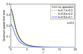
Figure 1: Quantum speed limit time as a function of initial time $\tau$ for sub Ohmic environment $s=0.5$ for different value of filtering operation parameter.

In Fig.(1), QSL time is plotted as a function of initial time $\tau$ for sub Ohmic environment $s=0.5$ for different value of filtering operation parameter $k$. It is obvious that the increasing of the filtering operation parameter in the region, $0.5<k<1$ leads to quantum speedup of quantum evolution. While increasing the filtering operation parameter in the region $0<k<0.5$ slowdown the quantum evolution.

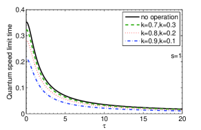
Figure 2: Quantum speed limit time as a function of initial time $\tau$ for Ohmic environment $s=1$ for different value of filtering operation parameter.

Fig.2, represents the QSL time for Ohmic environment $s=1$ with different value of filtering operation parameters. As can be seen, the QSL time is decreased by increasing of the filtering operation parameter in the region, $0.5<k<1$. So, in this region increasing filtering operation parameter speedup the quantum evolution. We also observe that the QSL time is increased by increasing filtering operation in the region $0<k<0.5$.

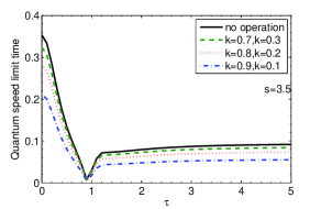
Figure 3: Quantum speed limit time as a function of initial time $\tau$ for super Ohmic environment $s=3.5$ for different value of filtering operation parameter.

Fig.3, shows the QSL time for super Ohmic environment $s=3.5$ with various value of filtering operation parameters. As can be seen, the QSL time is decreased by increasing of the filtering operation parameter in the region, $0.5<k<1$. We also observe that the QSL time is increased by increasing the filtering operation parameter in the region $0<k<0.5$. The fluctuation observed in the QSL time is due to the non-Markovian property of the noise.

III.2.2 dephasing model with colored noise

Now, we consider the interaction between a two-level quantum system with an environment which has the property of a random telegraph signal noise. The dynamics of quantum system is characterized by time dependent Hamiltonian

$$H(t)=\sum_{m=1}^{3}\Gamma_{m}(t)\sigma_{m},$$ (19)

where $\sigma_{m}$’s are the Pauli operators in ($x,y,z$) directions. $\Gamma_{m}(t)$’s are random variable which follow the statistics of a random telegraph signal. $\Gamma_{m}(t)$ depends on the random variable $n_{m}(t)$ as $\Gamma_{m}(t)=\alpha_{m}n_{m}(t)$, Where $n_{m}(t)$ has a Poisson distribution with an average value equal to $t/2\tau_{m}$ and $\alpha_{m}$’s are coin-flip random variables that randomly can have values $\pm\alpha_{m}$. Here, we consider dephasing model with colored noise with $\alpha_{1}=\alpha_{2}=0$ and $\alpha_{3}=\alpha$. In this model, the dynamics can be defined via the following Kraus operators

$$E_{1}(t)=\sqrt{\frac{1+\Lambda_{t}}{2}}\sigma_{0},\quad E_{2}(t)=\sqrt{\frac{1-\Lambda_{t}}{2}}\sigma_{3},\\$$ (20)

where $\Lambda_{t}=e^{-t/2\Delta}[\cos(\mu t/2\Delta)+\sin(\mu t/2\Delta)/\mu]$, $\mu=\sqrt{(4\alpha\Delta)^{2}-1}$. The dynamic is non-Markovian for $\alpha\Delta\geq 1/2$. After applying filtering operation on evolved density matrix, the final density matrix is obtained as

$$\rho_{f}(t)=\left(\begin{array}[]{cc}\frac{1-k}{2}&\frac{1}{2}\Lambda_{t}\sqrt{1-k}\sqrt{k}\\ \frac{1}{2}\Lambda_{t}\sqrt{1-k}\sqrt{k}&\frac{k}{2}\\ \end{array}\right),$$ (21)

From Eq.(8), the QSL time is obtained as

$$\tau_{QSL}=\sqrt{\frac{k(1-k)}{2}}\frac{\Lambda_{\tau}(\Lambda_{\tau+\tau_{D}}-\Lambda_{\tau})}{\frac{1}{\tau_{D}}\int_{\tau}^{\tau+\tau_{D}}\dot{\Lambda}_{t}dt}.$$ (22)

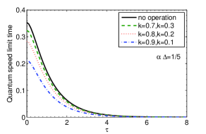
Figure 4: Quantum speed limit time as a function of initial time $\tau$ with $\alpha\Delta=1/5$ for different value of filtering operation parameter.

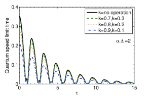
Figure 5: Quantum speed limit time as a function of initial time $\tau$ with $\alpha\Delta=2$ for different value of filtering operation parameter.

In Fig.(4), QSL time is plotted as a function of initial time $\tau$ for $\alpha\Delta=1/5$ with different value of filtering operation parameter $k$. It is obvious that the increasing of the filtering operation parameter in the region, $0.5<k<1$ leads to quantum speedup of quantum evolution. While the increasing of the filtering operation parameter in the region, $0<k<0.5$ leads to slowdown of quantum evolution.

Fig.5, represents the QSL time as a function of initial time for $\alpha\Delta=2$ with different value of filtering operation parameters. As can be seen, the QSL time is decreased by increasing of the filtering operation parameter in the region, $0.5<k<1$. While the QSL time is increased by increasing filtering operation parameter in the region, $0<k<0.5$. The fluctuation observed in the QSL time is due to the non-Markovian property of the noise.

IV Conclusion

In this work we investigated the effects of filtering operation on QSL time. We observed that the QSL time is decreased by increasing of the filtering operation parameter in the region, $0.5<k<1$. In other words in this region one can speedup the quantum evolution by increasing the filtering operation parameters. We can also observe that the quantum speed limit time is decreased by decreasing filtering operation parameter in the region, $0<k<0.5$. In other word, in this region one can slowdown the quantum evolution by increasing the filtering operation parameters.

References

- (1) L. M. Duan, M. D. Lukin, J. I. Cirac and P. Zoller, Nature 414, 413 (2001).
- (2) J. D. Bekenstein, Phys. Rev. Lett. 46, 623 (1981).
- (3) V. Giovannetti, S. Lloyd, and L. Maccone, Phys. Rev. Lett. 96, 010401 (2006).
- (4) V. Giovannetti, S. Lloyd and Lorenzo Maccone, Nat. Phot. 5, 222 (2011).
- (5) T. Caneva, et al, Phys. Rev. Lett. 103, 240501 (2009).
- (6) L. Mandelstam, I.G. Tamm : The uncertainty relation between energy and time in non-relativistic quantum mechanics. J. Phys. 9, 249 (1945).
- (7) N. Margolus, L.B. Levitin : The maximum speed of dynamical evolution. Physica (Amsterdam) 120 D, 188 (1998).
- (8) V. Giovannetti, S. Lloyd, L. Maccone : Quantum limits to dynamical evolution. Phys. Rev. A 67, 052109 (2003).
- (9) P. Jones, P. Kok : Geometric derivation of the quantum speed limit. Phys. Rev. A 82, 022107 (2010).
- (10) S. Deffner, E. Lutz : Energy-time uncertainty relation for driven quantum systems. J. Phys. A: Math. Theor. 46, 335302 (2013).
- (11) P. Pfeifer : How fast can a quantum state change with time? Phys. Rev. Lett. 70, 3365–3368 (1993).
- (12) P. Pfeifer, J. Frhlich : Generalized time-energy uncertainty relations and bounds on lifetimes of resonances. Rev. Mod. Phys. 67, 759–779 (1995).
- (13) M. M. Taddei, B. M. Escher, L. Davidovich, and R. L. de Matos Filho: Quantum speed limit for physical processes. Phys. Rev. Lett. 110, 050402 (2013).
- (14) A. del Campo, I. L. Egusquiza, M. B. Plenio, and S. F. Huelga: Quantum speed limits in open system dynamics. Phys. Rev. Lett. 110, 050403 (2013).
- (15) S. Deffner and E. Lutz : Quantum speed limit for non-Markovian dynamics. Phys. Rev. Lett. 111, 010402 (2013).
- (16) Y. Zhang, W. Han, Y. Xia, J. Cao, H. Fan : Quantum speed limit for arbitrary initial states. Sci. Rep. 4, 4890 (2014).
- (17) Yu. Min, Mao-Fa Fang, Zou. Hong-Mei : Quantum speed limit time of a two-level atom under differentquantum feedback control. Chin. Phys. B . 25(9): 090301 (2016).
- (18) Zhang, Y. J., Han, W., Xia, Y. J., Cao, J. P., Fan, H.: Classical-driving-assisted quantum speed-up. Phys. Rev. A 91 032112 (2015).
- (19) Y. J. Song, Q. S. Tan, L. M. Kuang : Control quantum evolution speed of a single dephasing qubit for arbitrary initial states via periodic dynamical decoupling pulses. Sci. Rep. 7 43654 (2017).
- (20) Y. N. Wu, J. Wang, H. Z. Zhang, : Quantum speedup of an atom coupled to a photonic-band-gap reservoir. Quantum Inf. Process 16 22 (2017).
- (21) Z.Y. Xu, S. Luo, W. L. Yang, C. Liu, S. Zhu : Quantum speedup in a memory environment. Phys, Rev. A 89, 012307 (2014).
- (22) JQ. Li, L. Bai, JQ. Liang: Entropic uncertainty relation under multiple bosonic reservoirs with filtering operator. Quantum Inf Process 17: 206 (2018).
- (23) G.M. Palma, K.A. Suominen, A.K. Ekert, Proc. R. Soc. Lond. A 452, 567–584 (1996).
- (24) S. Haseli, S. Salimi and A. S. Khorashad, Quantum Inf. Process. 14: 3581 (2015).