Deep Learning Enabled Semantic Communication Systems

Abstract

Recently, deep learned enabled end-to-end (E2E) communication systems have been developed to merge all physical layer blocks in the traditional communication systems, which make joint transceiver optimization possible. Powered by deep learning, natural language processing (NLP) has achieved great success in analyzing and understanding a large amount of language texts. Inspired by research results in both areas, we aim to provide a new view on communication systems from the semantic level. Particularly, we propose a deep learning based semantic communication system, named DeepSC, for text transmission. Based on the Transformer, the DeepSC aims at maximizing the system capacity and minimizing the semantic errors by recovering the meaning of sentences, rather than bit- or symbol-errors in traditional communications. Moreover, transfer learning is used to ensure the DeepSC applicable to different communication environments and to accelerate the model training process. To justify the performance of semantic communications accurately, we also initialize a new metric, named sentence similarity. Compared with the traditional communication system without considering semantic information exchange, the proposed DeepSC is more robust to channel variation and is able to achieve better performance, especially in the low signal-to-noise (SNR) regime, as demonstrated by the extensive simulation results.

.

I Introduction

BASED on Shannon and Weaver [1], communication could be categorized into three levels: i) transmission of symbols; ii) semantic exchange of transmitted symbols; iii) effects of semantic information exchange. The first level of communication mainly concerns about the successful transmission of symbols from the transmitter to the receiver, where the transmission accuracy is mainly measured at the level of bits or symbols. The second level of communication deals with the semantic information sent from the transmitter and the meaning interpreted at the receiver, named as semantic communication. The third level deals with the effects of communication that turn into the ability of the receiver to perform certain tasks in the way desired by the transmitter.

In the past decades, communications primarily focus on how to accurately and effectively transmit symbols (measured by bits) from the transmitter to the receiver. In such systems, bit-error rate (BER) or symbol-error rate (SER) is usually taken as the performance metrics [2]. With the development from the first generation (1G) to the fifth generation (5G), the achieved transmission rate has been improved tens of thousands of times and the system capacity is gradually approaching to the Shannon limit. Recently, various new applications appear, such as autonomous transportation, consumer robotics, environmental monitoring, and tele-health [3, 4]. The interconnection of these applications will generate a staggering amount of data in the order of zetta-bytes. Besides, these applications need to support massive connectivity over limited spectrum resources but require lower latency, which poses critical challenges to traditional source-channel coding. Semantic communications can process data in the semantic domain by extracting the meanings of data and filtering out the useless, irrelevant, and unessential information, which further compresses data while reserving the meanings. Moreover, semantic communication is expected to be robust to terrible channel environments, i.e., low signal-to-noise ratio (SNR) region, which fits well the applications requiring high reliability. These factors motivate us to develop intelligent communication systems by considering the semantic meaning behind digital bits to enhance the accuracy and efficiency of communications.

Different from the conventional communications, semantic communications aim to transmit the information relevant to the transmission goal. For example, for text transmission, the meaning is thereby essential information and the expression, i.e., is expression of word, are unnecessary. By doing so, the data traffic would be reduced significantly. Such a system could be particularly useful when the bandwidth is limited, the SNR is low, or the BER/SER is high in typical communication systems.

Historically, the concept of semantic communication was developed several decades ago. Inspired by Shannon and Weaver [1], Carnap et al. [5] were the first to introduce the semantic information theory (SIT) based on logical probabilities ranging over the contents. Afterwards, a generic model of semantic communication (GMSC) was proposed as an extension of the SIT, where the concepts of semantic noise and semantic channel were first defined [6]. As pointed out in [7], the analysis and design of a communication system for optimal transmission of intelligence are faced with several challenges. For instance, how to define error in the intelligence transmission? In [8], a lossless semantic data compression theory by applying the GMSC was developed, which means that data can be compressed at semantic level so that the size of the data to be transmitted can be reduced significantly. Recently, an end-to-end (E2E) semantic communication framework integrates the semantic inference and physical layer communication problems, where the transceiver is optimized to reach the Nash equilibrium while minimizing the average semantic errors [9]. However, the semantic error in [9] measures the meaning of each word rather than the whole sentence. These aforementioned works provide some insights and remarks for the design of semantic communications, but many issues remain unexplored.

Recent advancements on deep learning (DL) based natural language processing (NLP) and communication systems inspire us to investigate semantic communication to realize the second level communications as aforementioned [10, 11, 12, 13, 14, 15]. The considered semantic communication system mainly focuses on the joint semantic-channel coding and decoding, which aims to extract and encode the semantic information of sentences rather than simply a sequence of bits or a word. For the semantic communication system, we face the following questions:

• Question 1: How to define the meaning behind the bits?

• Question 2: How to measure the semantic error of sentences?

• Question 3: How to jointly design the semantic and channel coding?

In this paper, we investigate the semantic communication system by applying machine translation techniques in NLP to physical layer communications. Specifically, we propose a DL enabled semantic communication system (DeepSC) to address the aforementioned challenges. The main contributions of this paper are summarized as follows:

• Based on the Transformer [16], a novel framework for the DeepSC is proposed, which can effectively extract the semantic information from texts with robustness to noise. In the proposed DeepSC, a joint semantic-channel coding is designed to cope with channel noise and semantic distortion, which addresses aforementioned Question 3.

• The transceiver of the DeepSC is composed of semantic encoder, channel encoder, channel decoder, and semantic decoder. To understand the semantic meaning as well as maximize the system capacity at the same time, the receiver is optimized with two loss functions: cross-entropy and mutual information. Moreover, a new metric is proposed to accurately reflect the performance of the DeepSC at the semantic level. These address the aforementioned Questions 1 and 2.

• To make the DeepSC applicable to various communication scenarios, deep transfer learning is adopted to accelerate the model re-training. With the re-trained model, the DeepSC can recognise various knowledge input and recover semantic information from distortion.

• Based on extensive simulation results, the proposed DeepSC outperforms the traditional communication system and improves the system robustness at the low SNR regime.

The rest of this paper is organized as follows. Related work is briefly reviewed in Section II. The framework of a semantic communication system is presented and a corresponding problem is formulated in Section III. Section IV details the proposed DeepSC and extends it to dynamic environments. Numerical results are presented in Section VI to show the performance of the DeepSC. Finally, Section VII concludes this paper.

$Notation$: $\mathbb{C}^{n\times m}$ and $\mathbb{R}^{n\times m}$ represent sets of complex and real matrices of size $n\times m$, respectively. Bold-font variables denote matrices or vectors. $x\sim{\cal CN}(\mu,\sigma^{2})$ means variable $x$ follows a circularly-symmetric complex Gaussian distribution with mean $\mu$ and covariance $\sigma^{2}$. $(\cdot)^{T}$ and $(\cdot)^{H}$ denote the transpose and Hermitian, respectively. $\Re\{\cdot\}$ and $\Im\{\cdot\}$ refer to the real and imaginary parts of a complex number. Finally, ${\bf a}\otimes{\bf b}$ indicates the inner product of vectors $\bf a$ and $\bf b$.

II Related Work

This section provides a brief review of the related work on the E2E physical layer communication systems and the deep neural network (DNN) techniques adopted in NLP.

II-A End-to-End Physical Layer Communication Systems

DL techniques have shown great potential in processing various intelligent tasks, i.e., computer vision and NLP. Meanwhile, it is possible to train neural networks and run them on mobile devices due to the increasing hardware computing capability. In the communication area, some pioneering works have been carried on DL based E2E physical layer communication systems, which merge the blocks in traditional communication systems [17, 18, 19, 20, 21, 22, 23]. By adopting the structure of autoencoder in DL and removing block structure, the transmitter and receiver in the E2E system are optimized jointly as an E2E reconstruction task. It has been demonstrated that such an E2E system outperforms uncoded binary phase shift keying (BPSK) and Hamming coded BPSK in terms of BER [17]. Besides, there are several initial works on dealing with the missing channel gradient during training. A DNN based two-phase of training processing has been proposed, where the transceiver is trained by an stochastic channel model and the receiver is fine-tuned under real channels [18]. Reinforcement learning has been exploited in [19] to acquire the channel gradient under an unknown channel model, which achieves better performance than the differential quadrature phase-shift keying (DQPSK) over real channels. A conditional generative adversarial net (GAN) has been applied in [20] to use a DNN to represent the channel distortion so that the gradients can pass through a unknown channel to the transmitter DNN during the training of the E2E communication system. Meta-learning combined with a limited number of pilots has been developed for training the transceiver and enables the fast training of network with less amount of data [21].

Considering the types of sources, the joint source-channel coding for texts [22] and images [23] aims to recover the source information at the receiver directly rather than the digital bits. Meanwhile, traditional metrics, such as BER, cannot reflect the performance for such systems well. Therefore, word-error rate and peak signal-to-noise ratio (PSNR) are adopted for measuring the accuracy of source information recovery.

II-B Semantic Representation in Natural Language Processing

NLP makes machines understand human languages, with the main goal to understand the syntax and text. Initially, natural language can be described by the joint probability model according to the context [24]. Thus, language models provide context to distinguish words and phrases that have similar semantic meaning. Although such NLP technologies based on statistical model are developed to describe the probability of a certain word coming after another in a sentence, it is hard to deal with long sentences, i.e. the ones over 15 words, and the syntax. To understand long sentences, the word2vec model in [25] captures the relationship among words, which makes similar words ending up with a closer distance in the vector space. Even if these dense word vectors can capture the relationship among words, they fail to describe syntax information. In order to solve such problems, the underlying meaning of texts is represented by using various DL techniques, which is able to extract the semantic information in long sentences and their syntax. A deep contextualized word representation has been proposed in [26], which models both complex characteristics of word usages, e.g., syntax and semantics, and how these usages vary across linguistic contexts (i.e., to model polysemy). However, the above word representation approaches are designed for specific tasks and may need to be redesigned whenever the task changes. In [27], a general word representation model, named bidirectional encoder representations from transformers (BERT), has been developed to provide word vectors for various NLP tasks without requiring redesign of word representations.

II-C Comparison of State-of-Art NLP Techniques

There are three types of neural networks used for NLP tasks, including recurrent neural networks (RNNs), convolutional neural networks (CNNs) and fully-connected neural networks (FCNs) [28]. By introducing RNNs, language models can learn the whole sentences and capture the syntax information effectively [29]. However, for long sentences, particularly, the distance between subject and predicate is more than 10 words, RNNs cannot find the correct subject and predicate. For example, for sentence “the person who works in the new post office is walking to the store”, RNNs fail to recognise the relationship between “the person” and “is”. Besides, because of linear sequence structure, RNNs lack of parallel computing capability, which means that RNNs are time-consuming. CNNs were born with the capability of parallel computing [30]. However, even if CNNs can use deeper network to extract semantic information in long sentences, its performance is not as good as that of RNNs because the kernel size in CNNs is small to guarantee the computational efficiency. By combining with the attention mechanism, language models based on FCNs, such as Transformer [16], pay more attention to the useful semantic information for performance improvement on various NLP tasks. It is worth noting that the Transformer has the advantages of both RNNs and CNNs [16]. Particularly, the self-attention mechanism is adopted, which enables the models to understand sentences regardless of their lengths.

III System Model and Problem Formulation

The considered system model consists of two levels: semantic level and transmission level, as shown in Fig. 1. The semantic level addresses semantic information processing for encoding and decoding to extract the semantic information. The transmission level guarantees that semantic information can be exchanged correctly over the transmission medium. Overall, we consider an intelligent E2E communication system with the stochastic physical channel, where the transmitter and the receiver have certain background knowledge, i.e., different training data. The background knowledge could be various for different application scenarios.

Definition 1

Semantic noise is a type of disturbance in the exchange of a message that interferes with the interpretation of the message due to ambiguity in words, a sentence or symbols used in the message transmission.

Definition 2

Physical channel noise is caused by the physical channel impairment, such as, additive white Gaussian noise (AWGN), fading channel, and multiple path, which incurs the signal attenuation and distortion.

III-A Problem Description

As in Fig. 1, the transmitter maps a sentence, $\bf s$, into a complex symbol stream, $\bf x$, and then passes it through the physical channel with transmission impairments, such as distortion and noise. The received, $\bf y$, is decoded at the receiver to estimate the original sentence, ${\bf s}$. We jointly design the transmitter and receiver with DNNs since DL enables us to train a model with inputting variable-length sentences and different languages.

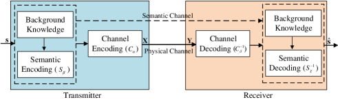
Figure 1: The framework of proposed DL enabled semantic communication system, DeepSC.

Particularly, we assume that the input of the DeepSC is a sentence, ${\mathbf{s}}=\left[{{w_{1}},{w_{2}},\cdots,{w_{L}}}\right]$, where $w_{l}$ represents the $l$-th word in the sentence. As shown in Fig. 1, the transmitter consists of two parts, named semantic encoder and channel encoder, to extract the semantic information from $\bf s$ and guarantee successful transmission of semantic information over the physical channel. The encoded symbol stream can be represented by

$${\mathbf{x}}={C_{{\bm{{\bm{\alpha}}}}}}\left({{S_{{{\bm{\beta}}}}}\left({\mathbf{s}}\right)}\right),$$ (1)

where ${\bf{x}}\in{\mathbb{C}^{M\times 1}}$, ${S_{{\bm{\beta}}}}\left(\cdot\right)$ is the semantic encoder network with the parameter set ${{\bm{\beta}}}$ and ${C_{\bm{\alpha}}}\left(\cdot\right)$ is the channel encoder with the parameter set $\mathbf{{\bm{\alpha}}}$. In order to simplify the analysis, we assume the coherent time is $M$. If $\bf x$ is sent, the signal received at the receiver will be

$${\bf{y}}=h{\bf{x}}+{\bf{n}},$$ (2)

where ${\bf{y}}\in{C^{M\times 1}}$, $h$ represents the Rayleigh fading channel with ${\cal CN}\left({0,1}\right)$ and ${\bf n}\sim{\cal CN}\left({0,\sigma_{n}^{2}}\right)$. For E2E training of the encoder and the decoder, the channel must allow back-propagation. Physical channels can be formulated by neural networks. For example, simple neural networks could be used to model the AWGN channel, multiplicative Gaussian noise channel, and the erasure channel [22]. While for the fading channels, more complicated neural networks are required [20]. In this paper, we mainly consider the AWGN channels and Rayleigh fading channels for simplicity while focus on semantic coding and decoding.

As shown in Fig. 1, the receiver includes channel decoder and semantic decoder to recover the transmitted symbols and then transmitted sentences, respectively. The decoded signal can be represented as

$${\mathbf{\hat{s}}}={S^{-1}_{\bm{\chi}}}\left({{C^{-1}_{\bm{\delta}}}\left({\mathbf{y}}\right)}\right),$$ (3)

where the $\bf\hat{s}$ is the recovered sentence, $C^{-1}_{\bm{\delta}}\left(\cdot\right)$ is the channel decoder with the parameter set ${\bm{\delta}}$ and $S^{-1}_{\bm{\chi}}\left(\cdot\right)$ is the semantic decoder network with the parameter set $\mathbf{{\bm{\chi}}}$.

The goal of the system is to minimize the semantic errors while reducing the number of symbols to be transmitted. However, we face two challenges in the considered system. The first challenge is how to design joint semantic-channel coding. The other one is semantic transmission, which has not been considered in the traditional communication system. Even if the existing communication system can achieve a low BER, several bits, distorted by the noise and beyond error correction capability, could lead to understanding difficulty as the partial semantic information of the whole sentence might be missed. In order to achieve successful recovery at semantic level, we design semantic and channel coding jointly in order to keep the meaning between $\hat{\bf s}$ and $\bf s$ unchanged, which is enabled by a new DNN framework. The cross-entropy (CE) is used as the loss function to measure the difference between $\bf s$ and $\bf\hat{s}$, which can be formulated as

$${\cal L}_{\rm CE}({\mathbf{s}},{\mathbf{\hat{s}}};{\bm{\alpha}},{\bm{\beta}},{\bm{\chi}},{\bm{\delta}})=$$ (4)

$$-\sum\limits_{l=1}{{q\left({{w_{l}}}\right)}\log\left({p\left({{w_{l}}}\right)}\right)}+(1-{q\left({{w_{l}}}\right)})\log\left({1-p\left({{w_{l}}}\right)}\right),$$

where $q(w_{l})$ is the real probability that the $l$-th word, $w_{l}$, appears in estimated sentence $\bf s$, and $p({w_{l}})$ is the predicted probability that the $i$-th word, $w_{i}$, appears in sentence $\hat{\bf s}$. The CE can measure the difference between two probability distributions. Through reducing the loss value of CE, the network can learn the word distribution, $q(w_{l})$, in the source sentence, $\bf s$, which indicates that the syntax, phrase, the meaning of words in context can be learnt by the network. Besides, jointly designing and training semantic-channel coding can make the whole network learning the knowledge for the specific goal. In other words, the channel coding can pay more attention in protecting the semantic information related to transmission goal while neglecting other irrelevant information. Separately designing will make channel coding addressing all information equally.

III-B Channel Encoder and Decoder Design

One important goal on designing a communication system is to maximize the capacity or the data transmission rate. Compared with BER, the mutual information can provide extra information to train a receiver. The mutual information of the transmitted symbols, $\bf x$, and the received symbols, $\bf y$, can be computed by

$$I\left({\bf x;y}\right) =\int{{}_{{\mathcal{X}}\times{\mathcal{Y}}}p\left({x,y}\right)\log\frac{{p\left({x,y}\right)}}{{p\left(x\right)p\left(y\right)}}}dxdy$$ (5)

$$={\mathbb{E}}_{p(x,y)}\left[{\log\frac{{p\left({x,y}\right)}}{{p\left(y\right)p\left(x\right)}}}\right],$$

where $(\bf x,\bf y)$ is a pair of random variables with values over the space ${{\mathcal{X}}\times{\mathcal{Y}}}$, where $\cal X$ and $\cal Y$ are the spaces for $\bf x$ and $\bf y$. $p(x)$ and $p(y)$ are the marginal probability of sending $\bf x$ and received $\bf y$, respectively, and $p(x,y)$ is the joint probability of $\bf x$ and $\bf y$. The mutual information is equivalent to the Kullback-Leibler (KL) divergence between the marginal probabilities and the joint probability, which is given by

$$I\left({\bf x;y}\right)={D_{\rm KL}}\left({p\left({x,y}\right)\left\|{p\left(x\right)p\left(y\right)}\right.}\right).$$ (6)

From [31], we have the following theorem,

Theorem 1

The KL divergence admits the following dual representation

$${D_{\rm KL}}\left({P\left\|Q\right.}\right)=\mathop{\sup}\limits_{T:\Omega\to R}{E_{P}}\left[T\right]-\log\left({{E_{Q}}\left[{{e^{T}}}\right]}\right),$$ (7)

where the supremum is taken over all functions $T$ such that the two expectations are finite.

According to Theorem 1, the KL divergence can also be represented as

$${D_{\rm KL}}\left({p\left({x,y}\right)\left\|{p\left(x\right)p\left(y\right)}\right.}\right)\geqslant{{\mathbb{E}}_{p\left({x,y}\right)}}\left[T\right]-\log\left({{{\mathbb{E}}_{p\left(x\right)p\left(y\right)}}\left[{{e^{T}}}\right]}\right).$$ (8)

Thus, the lower bound of $I\left({\bf x;y}\right)$ can be obtained from (6) and (8). In order to find a tight bound on the $I\left({\bf x;y}\right)$, an unsupervised method is used to train the network $T$, where $T$ can be approximated by neural network. Meanwhile, the expectation in (8) can be computed by sampling, which converges to the true value as the number of samples increases. Then, we can optimize the encoder by maximizing the mutual information defined in (8) and the related loss function can be given by

$${\cal L}_{\rm MI}({\bf x,y};T)={{\mathbb{E}}_{p\left({x,y}\right)}}\left[f_{T}\right]-\log\left({{{\mathbb{E}}_{p\left(x\right)p\left(y\right)}}\left[{{e^{f_{T}}}}\right]}\right),$$ (9)

where $f_{T}$ is composed by a neural network, in which the inputs are samples from $p(x,y)$, $p(x)$, and $p(y)$. In our proposed design, $\bf x$ is generated by the function $C_{\bm{\alpha}}$ and $S_{\bm{\beta}}$, thus the loss function can be represented by ${\cal L}_{\rm MI}({\bf x,y};T,{\bm{\alpha}},{\bm{\beta}})$ with

$${\cal L}_{\rm MI}({\bf x,y};T,{\bm{\alpha}},{\bm{\beta}})\leqslant I(\bf x;y).$$ (10)

From (10), the loss function can be used to train neural networks to get ${\bm{\alpha}}$, ${\bm{\beta}}$, and $T$. For example, the mutual information can be estimated by training network $T$ when the encoders $\bf{\bm{\alpha}}$ and $\bf{\bm{\beta}}$ are fixed. Similarly, the encoder can be optimized by training ${\bm{\alpha}}$ and ${\bm{\beta}}$ when the mutual information is obtained.

III-C Performance Metrics

Performance criteria are important to the system design. In the E2E communication system, the BER is usually taken as the training target by the transmitter and receiver, which sometimes neglects the other aspect goals of communication. For text transmission, BER cannot reflect performance well. Except from human judgement to establish the similarity between sentences, bilingual evaluation understudy (BLEU) score is usually used to measure the results in machine translation [32], which will be used as one of the performance metrics in this paper. However, the BLEU score can only compare the difference between words in two sentences rather than their semantic information. Therefore, we initialize a new metric, named sentence similarity, to describe the similarity level of two sentences in terms of their semantic information, which is introduced in the following. This provides a solution to Question 2.

III-C1 BLEU Score

Through counting the difference of $n$-grams between transmitted and received texts, where $n$-grams means that the size of a word group. For example, for sentence “weather is good today”, $1$-gram: “weather”, “is”, “good” and “today”, $2$-grams: “weather is”, “is good” and “good today”. The same rule applies for the rest.

For the transmitted sentence $\bf s$ with length $l_{\bf s}$ and the decoded sentence $\bf\hat{s}$ with length $l_{\bf\hat{s}}$, the BLEU can be expressed as

$$\log{\text{BLEU = min}}\left({1-\frac{l_{\bf\hat{s}}}{l_{\bf s}},0}\right)+\sum\limits_{n=1}^{N}{{u_{n}}\log{p_{n}}},$$ (11)

where $u_{n}$ is the weights of $n$-grams and $p_{n}$ is the $n$-grams score, which is

$${p_{n}}=\frac{{\sum\nolimits_{k}{\min\left({{C_{k}}\left({{\mathbf{\hat{s}}}}\right),{C_{k}}\left({\mathbf{s}}\right)}\right)}}}{{\sum\nolimits_{k}{\min\left({{C_{k}}\left({{\mathbf{\hat{s}}}}\right)}\right)}}},$$ (12)

where $C_{k}(\cdot)$ is the frequency count function for the $k$-th elements in $n$-th grams.

The output of BLEU is a number between 0 and 1, which indicates how similar the decoded text is to the transmitted text, with 1 representing highest similarity. However, few human translations will attain the score of 1 since word error may not make the meaning of a sentence different. For instance, the two sentences, “my car was parked there” and “my automobile was parked there”, have the same meaning but with different BLEU scores since they use different words. To characterize such a feature, we propose a new metric, the sentence similarity, at the sentence level in addition to the BLEU score.

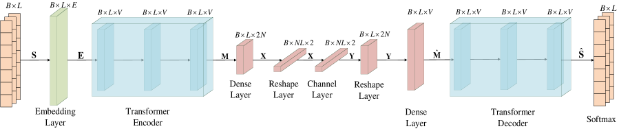
Figure 2: The proposed neural network structure for the semantic communication system.

III-C2 Sentence Similarity

A word can take different meanings in different contexts. For instance, the meanings of mouse in biology and machine are different. The traditional method, such as word2vec [25], cannot recognise the polysemy, of which the problem is how to use an numerical vector to express the word while the numerical vector varies in different contexts. According to the semantic similarity, we propose to calculate the sentence similarity between the original sentence, $\bf s$, and the recovered sentence, $\bf\hat{s}$, as

$${\text{match}}\left({\bf\hat{s},s}\right)=\frac{{{\bm{B}_{\bm{\Phi}}}\left({\bf{s}}\right)\cdot{\bm{B}_{\bm{\Phi}}}{{\left({{\bf{\hat{s}}}}\right)}^{T}}}}{{\left\|{{\bm{B}_{\bm{\Phi}}}\left({\bf{s}}\right)}\right\|\left\|{\bm{B_{\bm{\Phi}}}\left({{\bf{\hat{s}}}}\right)}\right\|}},$$ (13)

where ${\bm{B}_{\bm{\Phi}}}$, representing BERT [27], is a huge pre-trained model including billions of parameters used for extracting the semantic information. The sentence similarity defined in (13) is a number between 0 and 1, which indicates how similar the decoded sentence is to the transmitted sentence, with 1 representing highest similarity and 0 representing no similarity between $\bf s$ and $\bf\hat{s}$.

Compared with BLEU score, BERT has been fed by billions of sentences. Therefore, it has already learnt the semantic information from these sentences and can generate different semantic vectors in different contexts effectively. With the BERT, the semantic information behind a transmitted sentence, $\bf s$, can be expressed as $\bf c$. Meanwhile, the semantic information conveyed by the estimated sentence is expressed as $\bf\hat{c}$. For $\bf c$ and $\bf\hat{c}$, we can compute the sentence similarity by $\text{match}(\bf c,\bf\hat{c})$.

IV Proposed Deep Semantic Communication Systems

In this section, we propose a DNN for the considered semantic communication system, named as DeepSC, of which the Transformer is adopted for text understanding. Then, transfer learning is adopted to make the DeepSC applicable to different background knowledge and dynamic communication environments. This provides the solutions to Question 1,3.

IV-A Basic Model

The proposed DeepSC is as shown in Fig 2. Particularly, the transmitter consists of a semantic encoder to extract the semantic features from the texts to be transmitted and a channel encoder to generate symbols to facilitate the transmission subsequently. The semantic encoder includes multiple Transformer encoder layers and the channel encoder uses dense layers with different units. The AWGN channel is interpreted as one layer in the model. Accordingly, the DeepSC receiver is composited with a channel decoder for symbol detection and a semantic decoder for text estimation, the channel decoder includes dense layers with different units and the semantic decoder includes multiple Transformer decoder layers. The loss function can be expressed as

$${\cal L}_{\rm total}={\cal L}_{\rm CE}({\mathbf{s}},{\mathbf{\hat{s}}};{\bm{\alpha}},{\bm{\beta}},{\bm{\chi}},{\bm{\delta}})-\lambda{\cal L}_{\rm MI}({\bf x,y};T,{\bm{\alpha}},{\bm{\beta}}),$$ (14)

where the first term is the loss function considering the sentence similarity, which aims to minimize the semantic difference between $\bf s$ and $\bf\hat{s}$ by training the whole system. The second one is the loss function for mutual information, which maximize the achieved data rate during the transmitter training. The parameter $\lambda$ ($0\leq\lambda\leq 1$) is the weight for the second term.

The core of Transformer is the multi-head self-attention mechanism, which enables the Transformer to view the previous predicted word in the sequence, thereby better predicting the next word. Fig. 3 gives an example of the self-attention mechanism for the word ‘it’. From Fig. 3, attention attend to a distant dependency of the pronoun, ‘it’, completing pronoun reference “the animal”, which demonstrates that the self-attention mechanism can learn the semantic and therefore solve aforementioned Question 1.

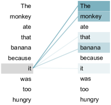
Figure 3: An example of the self-attention mechanism following long-distance dependency in the Transformer encoder.

Algorithm 1 DeepSC network training algorithm.

Initialization: Initial the weights $\bf W$ and bias $\bf b$.

1:  Input: The background knowledge set $\cal K$.

2:  Create the index to words and words to index, and then embedding words.

3:  while Stop criterion is not met do

4:     Train the mutual information estimated model.

5:     Train the whole network.

6:  end while

7:  Output: The whole network $S_{\bm{\beta}}(\cdot),C_{\bm{\alpha}}(\cdot),C^{-1}_{\bm{\delta}}(\cdot),S^{-1}_{\bm{\chi}}(\cdot)$.

As shown in Algorithm 1, the training process of the DeepSC consists of two phases due to different loss functions. After initializing the weights, $\bf W$, bias, $\bf b$, and using embedding vector to represent the input words, the first phase is to train the mutual information model by unsupervised learning to estimate the achieved data rate for the second phase. The second phase is to train the whole system with (14) as the loss function. Each phase aims to minimize the loss by gradient descent with mini-batch until the stop criterion is met, the max number of iteration is reached, or none of terms in the loss function is decreased any more. Different from performing semantic coding and channel coding separately, where the channel encoder/decoder will deal with the digital bits rather than the semantic information, the joint semantic-channel coding can preserve semantic information when compressing data, which provides the detailed solution for aforementioned Question 3. The two training phases are described in the following:

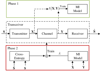
Figure 4: The training framework of the DeepSC: phase 1 trains the mutual information estimation model; phase 2 trains the whole network based on the cross-entropy and mutual information.

IV-A1 Training of mutual information estimation model

The mutual information estimation model training process is illustrated in Fig. 4 and the pseudocode is given in Algorithm 2. First, the knowledge set ${\cal K}$ generates a minibatch of sentences ${\mathbf{S}}\in{\Re^{B\times L\times 1}}$, where $B$ is the batch size, $L$ is the length of sentences. Through the embedding layer, the sentences can be represented as a dense word vector ${\bf E}\in{\Re^{B\times L\times E}}$, where $E$ is the dimension of the word vector. Then, pass the semantic encoder layer to obtain ${\bf M}\in{\Re^{B\times L\times V}}$, the semantic information conveyed by $\bf S$, where $V$ is the dimension of Transformer encoder’s output. Then, $\bf M$ is encoded into symbols ${\bf X}$ to cope with the effects from the physical channel, where ${\bf X}\in{\Re^{B\times NL\times 2}}$. After passing through the channel, the receiver obtains signal $\bf Y$ distorted by the channel noise. Based on (9), the loss, ${\cal L}_{\rm MI}({\bf X},{\bf Y};T,{\bm{\alpha}},{\bm{\beta}})$, can be computed based on the transmitted symbols, $\bf X$, and the received symbols, $\bf Y$, under the AWGN channels. Finally, according to computed ${\cal L}_{\rm MI}$, the stochastic gradient descent (SGD) is exploited to optimize the weights and bias of $f_{T}(\cdot)$.

Algorithm 2 Train mutual information estimation model.

1:  Input: The knowledge set $\cal K$.

2:  Transmitter:

3:    BatchSource(${\cal K}$) $\to$ $\bf S$.

4:    $S_{\bm{\beta}}(\bf S)\to{\bf M}$.

5:    $C_{\bm{\alpha}}(\bf M)\to{\bf X}$.

6:    Transmit $\bf X$ over the channel.

7:  Receiver:

8:    Receive $\bf Y$.

9:    Compute loss ${\cal L}_{\rm MI}$ by (9).

10:    Train $T$ $\to$ Gradient descent ($T,{\cal L}_{\rm MI}$).

11:  Output: The mutual information estimated model $f_{T}(\cdot)$.

IV-A2 Whole network training

The whole network training process is illustrated in Algorithm 3. First, minibatch $\bf S$ from knowledge $\cal K$ is encoded into $\bf M$ at the semantic level, then $\bf M$ is encoded into symbol ${\bf X}$ for transmission over the physical channels. At the receiver, distorted symbols $\bf Y$ are received and then decoded by the channel decoder layer, where ${\hat{\bf M}}\in{\Re^{B\times L\times V}}$ is the recovered semantic information of the sources. Afterwards, the transmitted sentences are estimated by the semantic decoder layer. Finally, the whole network is optimized by the SGD, where the loss is computed by (14).

Algorithm 3 Train the whole network.

1:  Input: The knowledge set $\cal K$.

2:  Transmitter:

3:    BatchSource(${\cal K}$) $\to$ $\bf S$.

4:    $S_{\bm{\beta}}(\bf S)\to{\bf M}$.

5:    $C_{\bm{\alpha}}(\bf M)\to{\bf X}$.

6:    Transmit $\bf X$ over the channel.

7:  Receiver:

8:    Receive $\bf Y$.

9:    $C^{-1}_{\bm{\delta}}(\bf Y)\to\hat{\bf M}$.

10:    $S^{-1}_{\bm{\chi}}({\hat{\bf M}})\to\hat{\bf S}$.

11:    Compute loss function ${\cal L}_{\rm total}$ by (14).

12:    Train ${\bm{\beta}},{\bm{\alpha}},{\bm{\delta}},{\bm{\chi}}$ $\to$ Gradient descent (${\bm{\beta}},{\bm{\alpha}},{\bm{\delta}},$ ${\bm{\chi}},{\cal L}_{\rm total}$).

13:  Output: The whole network $S_{\bm{\beta}}(\cdot),C_{\bm{\alpha}}(\cdot),C^{-1}_{\bm{\delta}}(\cdot),S^{-1}_{\bm{\chi}}(\cdot)$.

IV-B Transfer Learning for Dynamic Environment

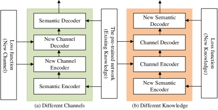
Figure 5: Transfer learning based training framework: (a) re-train channel encoder and decoder for different channels; (b) re-train semantic encoder and decoder for different background knowledge.

Algorithm 4 Transfer learning based training for dynamic environment.

Initialization: Load the pre-trained model $S_{\bm{\beta}}(\cdot),C_{\bm{\alpha}}(\cdot)$,
$C^{-1}_{\bm{\delta}}(\cdot),S^{-1}_{\bm{\chi}}(\cdot)$.

0:  Training for different background knowledge

1:  Input: The different background knowledge set ${\cal K}_{1}$ .

2:  Freeze $C_{\bm{\alpha}}(\cdot)$ and $C^{-1}_{\bm{\delta}}(\cdot)$.

3:  Redesign and train part of $S_{\bm{\beta}}(\cdot)$ and $S^{-1}_{\bm{\chi}}(\cdot)$.

4:  while Stop criterion is not met do

5:     Train the mutual information estimated model.

6:     Train the whole network.

7:  end while

8:  Output: The adopted whole network.

8:  Training for different channel conditions

9:  Input: The background knowledge set $\cal K$ with the different channel parameters.

10:  Freeze $S_{\bm{\beta}}(\cdot)$ and $S^{-1}_{\bm{\chi}}(\cdot)$.

11:  Redesign and re-train part of $C_{\bm{\alpha}}(\cdot)$ and $C^{-1}_{\bm{\delta}}(\cdot)$.

12:  while Stop criterion is not met do

13:     Train the mutual information estimated model.

14:     Train the whole network.

15:  end while

16:  Output: The re-trained network.

In practice, different communication scenarios result in the different channels and the training data. However, the re-training of transmitter and receiver to meet the requirements of dynamic scenarios introduces extra costs. To address this, a deep transfer learning approach is adopted, which focuses on storing knowledge gained while solving a problem and applying it to a different but related problem.

The training process of adopting transfer learning is illustrated in Fig. 5 and the pseudocode is given in Algorithm 4, where the training modules, mutual information estimation model training, and whole network training, are the same as Algorithm 2 and Algorithm 3. First, load the pre-trained transmitter and receiver based on knowledge ${\cal K}_{0}$ and channel ${\cal N}_{0}$. For applications with different background knowledge, we only need to redesign and train part of the semantic encoder and decoder layers and freeze the channel encoder and decoder layers. For different communication environments, we redesign and train part of the channel encoder and decoder layers and freeze the semantic encoder and decoder layers. If the knowledge and channel are totally different, the pre-trained transceiver can also reduce the time consumption because the weights of some layers in the pre-trained model can be reused in the new model even if the most layers need to redesign. After the other modules are trained, we will unfreeze them and train the whole network with few epochs to converge to the global optimum.

V Numerical Results

In this section, we compare the proposed DeepSC with other DNN algorithms and the traditional source coding and channel coding approaches under the AWGN channels and Rayleigh fading channels, where we assume perfect CSI for all schemes. The transfer learning aided DeepSC is also verified under the erase channel and fading channel as well as different background knowledge.

V-A Simulation Settings

The adopted dataset is the proceedings of the European Parliament [33], which consists of around 2.0 million sentences and 53 million words. The dataset is pre-processed into lengths of sentences with 4 to 30 words and is split into training data and testing data.

In the experiment, we set three Transformer encoder and decoder layer with 8 heads and the channel encoder and decoder are set as dense with 16 units and 128 units, respectively. For the mutual information estimation model, we set two dense layers with 256 units and one dense layer with 1 unit to mimic the function $T$ in (7), where 256 units can extract full information and 1 unit can integrate information. These settings can be found in Table V-B. For the baselines, we adopt joint source-channel coding based on neural network and the typical methods for separate source and channel codings.

• DNN based joint source-channel coding [22]: The network consists of Bi-directional Long Short-Term Memory (BLSTM) layers. We label it as JSCC [22] in the simulation figures.

• Traditional methods: To perform the source and channel coding separately, we use the following technologies respectively:

  • Source coding: Huffman coding, fixed-length coding (5-bit), and Brotli coding, where Brotli coding uses 2nd context model to compress the context information and every 128 sentences are compressed together in the simulation.

  • Channel coding: Turbo coding [34] and Reed-Solomon (RS) coding [35]. We adopt turbo decoding method is log-MAP algorithm with 5 iterations.

The BLEU and sentence similarity are used to measure the performance. The simulation is performed by the computer with Intel Core i7-9700 CPU@3.00GHz and NVIDIA GeForce GTX 2060.

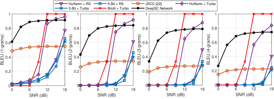
(a) AWGN

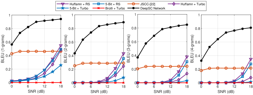
(b) Rayleigh Fading

Figure 6: BLEU score versus SNR for the same total number of transmitted symbols, with Huffman coding with RS (30,42) in 64-QAM, 5-bit coding with RS (42, 54) in 64-QAM, Huffman coding with Turbo coding in 64-QAM, 5-bit coding with Turbo coding in 128-QAM, Brotli coding with Turbo coding in 8-QAM; the DNN based JSCC [22] trained over the AWGN channels and Rayleigh fading channels, our proposed DeepSC trained over the AWGN channels and Rayleigh fading channels.

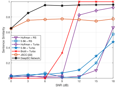
(a) AWGN

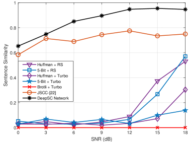
(b) Rayleigh Fading

Figure 7: Sentence similarity versus SNR for the same total number of transmitted symbols, with Huffman coding with RS (30,42) in 64-QAM; 5-bit coding with RS (42, 54) in 64-QAM; Huffman coding with Turbo coding in 64-QAM; 5-bit coding with Turbo coding in 128-QAM; Brotli coding with Turbo coding in 8-QAM; an E2E trained over the AWGN channels and Rayleigh fading channels  [22]; our proposed DeepSC trained over the AWGN channels and Rayleigh fading channels.

V-B Basic Model

Fig. 6 shows the relationship between the BLEU score and the SNR under the same number of transmitted symbols over AWGN and Rayleigh fading channels, where the traditional approaches use 8-QAM, 64-QAM, and 128-QAM for the modulation. Among the traditional baselines in Fig. 6(a), Brotli coding outperforms the Huffman and fixed-length encoding over AWGN channels when the turbo coding is adopted for channel coding. The traditional approaches perform better than the DNN based method when the SNR is above 12 dB since the distortion from channel is decreased, where the Brotli with turbo coding performs better than the DeepSC. We observe that all DL enabled approaches are more competitive in the low SNR regime.

Table I: The setting of the developed semantic network.

	Layer Name	Units	Activation
Transmitter (Encoder)	3$\times$Transformer Encoder	128 (8 heads)	Linear
	Dense	256	Relu
	Dense	16	Relu
Channel	AWGN	None	None
Receiver (Decoder)	Dense	256	Relu
	Dense	128	Relu
	3$\times$Transformer Decoder	128 (8 heads)	Linear
	Prediction Layer	Dictionary Size	Softmax
MI Model	Dense	256	Relu
	Dense	256	Relu
	Dense	1	Relu

In Fig. 6(b), the DL enabled approaches outperform all traditional approaches over the Rayleigh fading channels, where RS coding is better than turbo coding in terms of 2-grams to 4-grams. This is because RS coding is linear block coding with long block-length, and can correct long series of bits, however, turbo coding is a type of convolutional coding with short block-length, so that the adjacent words have higher error rate. DeepSC is not only suitable for short block-length but also performs better in decoding adjacent words, i.e., 4-grams. Note that the BLEU score of the method with Brotil coding and turbo coding is always 0 over Rayleigh fading channels. This is because that 128 sentences are compressed together, while Brotil decoding requires error-free codes after channel decoding for the codes corresponding to the 128 sentences. However, it is almost to guarantee the error-free transmission over Rayleigh fading channels. Therefore, we fail to restore any of the 128 sentences compressed together in Brotil coding as shown in Fig. 6(b). Besides, the lower BLEU score of the DL enabled approaches may not be caused by word errors. For example, it may be due to substitutions of words using synonyms or rephrasing, which does not change the meaning of the word. Fig. 6 also demonstrates that the joint semantic-channel coding design outperforms the traditional methods, which provides solution to Question 1 and 3.

Table II: The sample sentences between different methods over Rayleigh fading channels when SNR is 18 $dB$.

Transmitted sentence	it is an important step towards equal rights for all passengers.
DeepSC	it is an important step towards equal rights for all passengers.
JSCC-[22]	it is an essential way towards our principles for democracy.
Huffman + Turbo coding	rt is a imeomant step tomdrt equal rights for atp passurerrs.
Huffman + RS coding	it is an important step towards ewiral rlrsuo for all passengess.
Bit5 + Turbo coding	it is an yoportbnt ssep sowart euual qighd fkr ill passeneers.
Bit5 + RS coding	it iw an ymp!rdbnd stgo to!atds eq.al ryghts dkr alk passengers.

Fig. 7 shows that the proposed performance metric, the sentence similarity, with respect to the SNR under the same total number of symbols, where the traditional approaches use 8-QAM, 64-QAM and 128-QAM. In Fig. 7(a), the proposed metric has shown the same tendency compared with the BLEU scores. Note that for part of the traditional methods, i.e., Huffman with Turbo coding, even if it can achieve about 20% word accuracy in BLEU score (1-gram) from Fig. 6(a) when SNR = 9 dB, people are usually unable to understand the meaning of texts full of errors. Thus, the sentence similarity in Fig. 7(a) almost converges to 0. For the DeepSC, it achieves more than 90% word accuracy in BLEU score (1-gram) when SNR is higher than 6 dB in Fig. 6(a), which means people can understand the texts well. Therefore the sentence similarity tends to 1. Fig. 6(b) and Fig. 7(b) show the same tendency. The benchmark, including the DNN based JSCC method in [22] under Rayleigh fading channels, also gets much higher score than the traditional approaches in terms of the sentence similarity since it can capture the features of the syntax and the relationship of the words, as well as present texts that is easier for people to understand. Few representative results are shown in Table II.

In brief, we can conclude that the tendency in sentence similarity is more closer to human judgment and the DeepSC achieves the best performance in terms of both BLEU score and sentence similarity. Compared to the simulation results with BLEU score as the metric, the sentence similarity score can better measure the semantic error, which solves the Question 2.

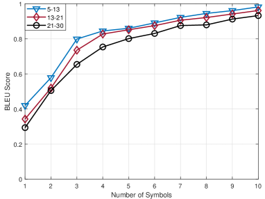
Figure 8: BLEU score (1-gram) versus the average number of symbols used for one word in the DeepSC, SNR = 12 dB.

Fig. 8 illustrates that the impact of the number of symbols per word on the 1-gram BLEU score when SNR is 12 dB. As the number of symbols per word grows, the BLEU scores increase significantly due to the increasing distance between constellations gradually. Generally, people can understand the basic meaning of transmitted sentences with over 85% word accuracy in BLEU score (1-gram). For short sentences consisted of 5 to 13 words, our proposed DeepSC can achieve 85% accuracy with 4 symbols per word, which means that we can use fewer symbols to represent one word in the environment that mainly transmits short sentences. Therefore, it can achieve high speed transmission rate. For longer sentences consisted from of 21 to 30 words, the proposed DeepSC faces more difficulties to understand the complex structure of the sentences in the transmitted texts. Hence the performance is degraded with longer sentences. One way to improve the BLEU score is to increase the average number of symbols used for each word.

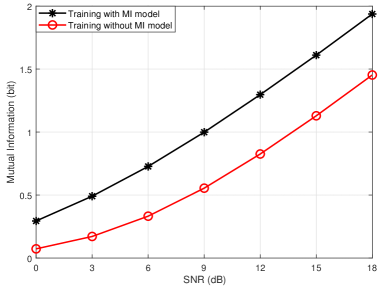
Figure 9: SNR versus mutual information for different trained encoders, with 8 symbols per word.

V-C Mutual Information

Fig. 9 demonstrates the relationship between SNR and mutual information after training. As we can imagine, the mutual information increases with SNR. From the figure, the performance of the transceiver trained with the mutual information estimation model outperforms that without such a model. From Fig. 9, with the proposed mutual information estimation model, the obtained mutual information at SNR = 4 dB is approximately same as that without the training model at SNR = 9dB. From another point of view, the mutual information estimation model leads to better learning results, i.e., data distribution, at the encoder to achieve higher data rate. In addition, this shows that introducing (9) in loss function can improve the mutual information of the system.

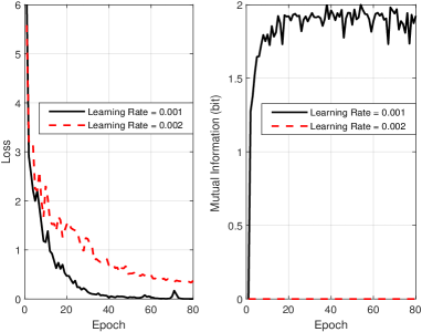
Figure 10: The impact of different learning rates with training SNR = 12 dB.

Fig. 10 draws the relationship between the loss value in (14) and the mutual information with increasing epoch. Fig. 12 indicates the relationship between BLEU score and SNR. The two figures are based on models with the same structure but different training parameters, i.e., learning rate. In Fig. 10, the obtained mutual information is different, i.e., the mutual information of model with learning rate 0.001 increases along with decreasing loss value while the other one with learning rate 0.002 stays zero although the loss values of two models gradually converge to a stable state. From Fig. 12, the BLEU score with learning rate 0.001 outperforms that with learning rate 0.002, which means that even if the neural network converges to a stable state, it is possible that gradient decreases to a local minimum instead of the global minimum. During the training process, the mutual information can be used as a tool to decide whether the model converges effectively.

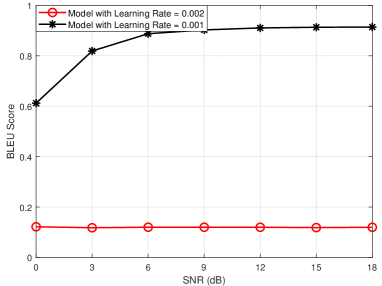
Figure 11: BLEU score (1-gram) versus SNR for different learning rates, with training SNR = 12 dB.

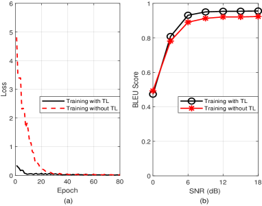
Figure 12: Transfer learning (TL) aided DeepSC with different background knowledge: (a) loss values versus the number of training epochs, (b) BLEU score (1-gram) versus the SNR.

V-D Transfer Learning for Dynamic Environment

In this experiment, we present the performance of transfer learning aided DeepSC for two tasks: transmitter and receiver re-training over different channels and diffident background knowledge.

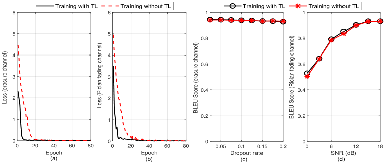
Figure 13: Transfer learning aided DeepSC with different channels: (a) loss values versus epochs under the erasure channel; (b) Loss values versus epochs under the Rician fading channel; (c) BLEU score (1-gram) versus the dropout rate; (d) BLEU score (1-gram) versus the SNR.

Fig. 12 shows the training efficiency and the performance for different background knowledge, where the model will be trained and re-trained in new background knowledge with the same channel (AWGN) for different background knowledge. The models have the same structure and re-train with the same parameters in each scenario. From Fig. 12(a), the epochs are reduced from 30 to 5 to reach convergence. In Fig. 12(b), the pre-trained model can provide additional knowledge so that the corresponding model training outperforms that of re-training the whole system. This demonstrates that the transfer learning aided DeepSC can help the transceiver to accommodate the new requirements of communication environment.

Fig. 13 shows the training efficiency and the performance for different channels, where the DeepSC transceiver is pre-trained under the AWGAN channel, and then it is re-trained under the erasure channel and the Rician fading channel, respectively, with the same background knowledge. The models have the same structure and re-train with the same parameters in each scenario. From Fig. 13(a) and Fig. 13(b), the adoption of the pre-trained model can speed up the training process for both the erasure channel and Rician fading channel. In Fig. 13(c) and Fig. 13(d), the performance of the DeepSC with pre-trained model is similar to that without pre-trained model channel while the required complexity is reduced significantly as less number of epochs is required during the re-training process. It is further noted that the BLEU score achieved by the DeepSC is slightly degraded under the fading channel, especially in the lower SNR region, compared to that under the erasure channel.

V-E Complexity Analysis

The computational complexities of the proposed DeepSC, the JSCC in [22], the RS coding, Turbo coding, are compared in Table III in terms of the average processing runtime per sentence. All the DL enabled approaches have lower runtime than the traditional approaches, where turbo coding costs much longer runtime in log-map iterations and the JSCC [22] requires the lowest average time due to its simple network architecture, however, it comes with poorer semantic processing capability. As a comparison, the runtime of our proposed DeepSC significantly outperforms the traditional schemes and is slight higher than JSCC [22] but with significant performance improvement.

Table III: The average sentence processing runtime versus various schemes.

	DeepSC	JSCC [22]	RS coding	Turbo coding
Runtime	3.27ms	2.71ms	4.14ms	8.59ms

VI Conclusions

In this paper, we have proposed a semantic communication system, named DeepSC, which jointly performs the semantic-channel coding for texts transmission. With the DeepSC, the length of input texts and output symbols are variable, and the mutual information is considered as a part of the loss function to achieve higher data rate. Besides, the deep transfer learning has been adopted to meet different transmission conditions and speed up the training of new networks by exploiting the knowledge from the pre-trained model. Moreover, we initialized sentence similarity as a new performance metric for the semantic error, which is a measure closer to human judgement. The simulation results has demonstrated that the DeepSC outperforms various benchmarks, especially in the low SNR regime. The proposed transfer learning aided DeepSC has shown its ability to adapt to different channels and knowledge with fast convergence speed. Therefore, our proposed DeepSC is a good candidate for text transmission, especially in the low SNR regime, which could be very useful for cases with massive number of devices to be connected with the limited spectrum resource.

We conclude the difference between semantic communication systems and conventional communication systems into the following:

1. Different data processing domains. The former process data in semantic domain while the latter compress data in entropy domain.

2. Different communication targets. The conventional communication systems focus on the exact data recovery while the semantic communication systems serve for the decisions or targets of the transmission.

3. Different system designs. The conventional systems only design and optimize the information transmission modules, which are contained in the traditional transceiver, however, the semantic systems jointly design the whole information processing blocks from source information to final targets of applications.

Following the concept of semantic communications proposed in this paper, we have developed L-DeepSC [36] and DeepSC-S [37] for text and speech transmission.

References

- [1] C. E. Shannon and W. Weaver, The Mathematical Theory of Communication. The University of Illinois Press, 1949.
- [2] D. Tse and P. Viswanath, Fundamentals Wireless Communication. Cambridge University Press, 2005.
- [3] L. Atzori, A. Iera, and G. Morabito, “The internet of things: A survey,” Computer Networks, vol. 54, no. 15, pp. 2787–2805, May 2010.
- [4] F. Jameel, Z. Chang, J. Huang, and T. Ristaniemi, “Internet of autonomous vehicles: architecture, features, and socio-technological challenges,” IEEE Wireless Commun., vol. 26, no. 4, pp. 21–29, 2019.
- [5] R. Carnap, Y. Bar-Hillel et al., An Outline of A Theory of Semantic Information. RLE Technical Reports 247, Research Laboratory of Electronics, Massachusetts Institute of Technology., Cambridge MA, Oct. 1952.
- [6] J. Bao, P. Basu, M. Dean, C. Partridge, A. Swami, W. Leland, and J. A. Hendler, “Towards a theory of semantic communication,” in IEEE Network Science Workshop, West Point, NY, USA, Jun. 2011, pp. 110–117.
- [7] B. H. Juang, “Quantification and transmission of information and intelligence—history and outlook [DSP history],” IEEE Signal Processing Mag., vol. 28, no. 4, pp. 90–101, Jul. 2011.
- [8] P. Basu, J. Bao, M. Dean, and J. Hendler, “Preserving quality of information by using semantic relationships,” Pervasive Mob. Comput., vol. 11, pp. 188–202, Apr. 2014.
- [9] B. Guler, A. Yener, and A. Swami, “The semantic communication game,” IEEE Trans. Cogn. Comm. Networking, vol. 4, no. 4, pp. 787–802, Sep. 2018.
- [10] D. Bahdanau, K. Cho, and Y. Bengio, “Neural machine translation by jointly learning to align and translate,” in Proc. Int’l. Conf. Learning Representations (ICLR’15), San Diego, CA, USA, May 2015.
- [11] E. Cambria and B. White, “Jumping NLP curves: A review of natural language processing research [review article],” IEEE Comput. Intell. Mag., vol. 9, no. 2, pp. 48–57, Apr. 2014.
- [12] N. Farsad and A. Goldsmith, “Neural network detection of data sequences in communication systems,” IEEE Trans. Signal Process., vol. 66, no. 21, pp. 5663–5678, Sep. 2018.
- [13] H. He, C. Wen, S. Jin, and G. Y. Li, “Model-driven deep learning for MIMO detection,” IEEE Trans. Signal Process., vol. 68, pp. 1702–1715, Feb. 2020.
- [14] H. Sun, X. Chen, Q. Shi, M. Hong, X. Fu, and N. D. Sidiropoulos, “Learning to optimize: Training deep neural networks for interference management,” IEEE Trans. Signal Process., vol. 66, no. 20, pp. 5438–5453, Aug. 2018.
- [15] Z. Qin, H. Ye, G. Y. Li, and B.-H. F. Juang, “Deep learning in physical layer communications,” IEEE Wireless Commun., vol. 26, no. 2, pp. 93–99, Apr. 2019.
- [16] A. Vaswani, N. Shazeer, N. Parmar, J. Uszkoreit, L. Jones, A. N. Gomez, Ł. Kaiser, and I. Polosukhin, “Attention is all you need,” in Advances Neural Info. Process. Systems (NIPS’17), Long Beach, CA, USA. Dec. 2017, pp. 5998–6008.
- [17] T. O’Shea and J. Hoydis, “An introduction to deep learning for the physical layer,” IEEE Trans. Cogn. Comm. & Networking, vol. 3, no. 4, pp. 563–575, Oct. 2017.
- [18] S. Dörner, S. Cammerer, J. Hoydis, and S. ten Brink, “Deep learning based communication over the air,” IEEE J. Sel. Topics Signal Processing, vol. 12, no. 1, pp. 132–143, Dec. 2018.
- [19] F. A. Aoudia and J. Hoydis, “Model-free training of end-to-end communication systems,” IEEE J. Sel. Areas Commun., vol. 37, no. 11, pp. 2503–2516, Aug. 2019.
- [20] H. Ye, L. Liang, G. Y. Li, and B. Juang, “Deep learning based end-to-end wireless communication systems with conditional GAN as unknown channel,” IEEE Trans. Wireless Commun., vol. 19, no. 5, pp. 3133–3143, Feb. 2020.
- [21] S. Park, O. Simeone, and J. Kang, “End-to-end fast training of communication links without a channel model via online meta-learning,” arXiv preprint arXiv:2003.01479, Mar. 2020.
- [22] N. Farsad, M. Rao, and A. Goldsmith, “Deep learning for joint source-channel coding of text,” in Proc. IEEE Int’l. Conf. Acoustics Speech Signal Process. (ICASSP’18), Calgary, AB, Canada, Apr. 2018, pp. 2326–2330.
- [23] E. Bourtsoulatze, D. B. Kurka, and D. Gündüz, “Deep joint source-channel coding for wireless image transmission,” IEEE Trans. Cogn. Comm.Networking, vol. 5, no. 3, pp. 567–579, May 2019.
- [24] R. Kneser and H. Ney, “Improved backing-off for M-gram language modeling,” in Proc. IEEE Int’l. Conf. Acoustics Speech Signal Process. (ICASSP’95), Detroit, Michigan, USA, May 1995, pp. 181–184.
- [25] T. Mikolov, K. Chen, G. Corrado, and J. Dean, “Efficient estimation of word representations in vector space,” in Proc. Int’l. Conf. Learning Representations (ICLR’13), Scottsdale, Arizona, USA, May 2013.
- [26] M. E. Peters, M. Neumann, M. Iyyer, M. Gardner, C. Clark, K. Lee, and L. Zettlemoyer, “Deep contextualized word representations,” in Proc. North American Chapter of the Assoc. for Comput. Linguistics: Human Language Tech., (NAACL-HLT’18), New Orleans, Louisiana, Jun. 2018, pp. 2227–2237.
- [27] J. Devlin, M. Chang, K. Lee, and K. Toutanova, “BERT: pre-training of deep bidirectional transformers for language understanding,” in Proc. North American Chapter of the Assoc. for Comput. Linguistics: Human Language Tech., (NAACL-HLT’19), Minneapolis, MN, USA, Jun. 2019, pp. 4171–4186.
- [28] M. Schuster and K. K. Paliwal, “Bidirectional recurrent neural networks,” IEEE Trans. Signal Process., vol. 45, no. 11, pp. 2673–2681, Nov. 1997.
- [29] A. Graves, “Generating sequences with recurrent neural networks,” arXiv preprint arXiv:1308.0850, Aug. 2013.
- [30] N. Kalchbrenner, E. Grefenstette, and P. Blunsom, “A convolutional neural network for modelling sentences,” in Proc. Annual Meeting Assoc. Comput. Linguistics (ACL’14), Baltimore, MD, USA, Jun. 2014, pp. 655–665.
- [31] M. I. Belghazi, A. Baratin, S. Rajeshwar, S. Ozair, Y. Bengio, A. Courville, and D. Hjelm, “Mutual information neural estimation,” in Int’l. Conf. Machine Learning (ICML’18), Stockholm, Sweden, Jul. 2018, pp. 531–540.
- [32] K. Papineni, S. Roukos, T. Ward, and W. Zhu, “Bleu: a method for automatic evaluation of machine translation,” in Proc. Annual Meeting Assoc. Comput. Linguistics (ACL’02), Philadelphia, PA, USA, Jul. 2002, pp. 311–318.
- [33] P. Koehn, “Europarl: A parallel corpus for statistical machine translation,” in MT summit, vol. 5. Citeseer, Sep. 2005, pp. 79–86.
- [34] C. Heegard and S. B. Wicker, Turbo coding. Springer Science & Business Media, 2013, vol. 476.
- [35] I. S. Reed and G. Solomon, “Polynomial codes over certain finite fields,” J. the Society for Industrial and Applied Math., vol. 8, no. 2, pp. 300–304, Jan. 1960.
- [36] H. Xie and Z. Qin, “A lite distributed semantic communication system for internet of things,” IEEE J. Sel. Areas Commun., vol. 39, no. 1, pp. 142–153, Jan. 2021.
- [37] Z. Weng, Z. Qin, and G. Y. Li, “Semantic communications for speech signals,” in Proc. IEEE Int’l. Conf. on Comm. (ICC’21), Montreal, Canada, Jun 2021.