Tight Bounds for the Probability of Connectivity
in Random K-out Graphs

Abstract

Random K-out graphs are used in several applications including modeling by sensor networks secured by the random pairwise key predistribution scheme, and payment channel networks. The random K-out graph with $n$ nodes is constructed as follows. Each node draws an edge towards $K$ distinct nodes selected uniformly at random. The orientation of the edges is then ignored, yielding an undirected graph. An interesting property of random K-out graphs is that they are connected almost surely in the limit of large $n$ for any $K\geq 2$. This means that they attain the property of being connected very easily, i.e., with far fewer edges ($O(n)$) as compared to classical random graph models including Erdős-Rényi graphs ($O(n\log n)$). This work aims to reveal to what extent the asymptotic behavior of random K-out graphs being connected easily extends to cases where the number $n$ of nodes is small. We establish upper and lower bounds on the probability of connectivity when $n$ is finite. Our lower bounds improve significantly upon the existing results, and indicate that random K-out graphs can attain a given probability of connectivity at much smaller network sizes than previously known. We also show that the established upper and lower bounds match order-wise; i.e., further improvement on the order of $n$ in the lower bound is not possible. In particular, we prove that the probability of connectivity is $1-\Theta({1}/{n^{K^{2}-1}})$ for all $K\geq 2$. Through numerical simulations, we show that our bounds closely mirror the empirically observed probability of connectivity.

I Introduction

Random graphs constitute an important framework for analyzing the underlying structural characteristics of complex real-world networks such as communication networks, social networks and biological networks[1, 2, 3]. A class of random graphs called the random K-out graphs is one of the earliest known models of random graphs [4, 5]. The random K-out graph comprising $n$ nodes, denoted by $\mathbb{H}(n;K)$, is constructed as follows. Each node draws $K$ edges towards $K$ distinct nodes chosen uniformly at random from all other nodes. The orientation of the edges is then ignored, yielding an undirected graph. Due to their unique connectivity properties, random K-out graphs have received renewed interest for analyzing secure wireless sensor networks and routing in cryptocurrency networks.

In the context of wireless sensor networks (WSNs), random K-out graphs have been used extensively for evaluating strategies for secure communication. The limited computation and communication capabilities of WSNs precludes the use of traditional key exchange protocols for establishing secure connectivity [6, 7, 8]. Moreover, WSNs deployed for applications such as battlefield surveillance and environmental monitoring are vulnerable to adversarial attacks and operational failures. For facilitating secure connectivity in WSNs, Eschenauer and Gligor [6] proposed the random predistribution of symmetric cryptographic keys. Subsequently, several variants of random key predistribution schemes have been studied; see [9, 8] and the references therein. A widely adopted approach is the random pairwise key predistribution introduced by Chan et al. [10]. The random pairwise scheme is implemented in two phases. In the first phase, each sensor node is paired offline with $K$ distinct nodes chosen uniformly at random among all other sensor nodes. Next, a unique pairwise key is inserted in the memory of each of the paired sensors. After deployment, two sensor nodes can communicate securely only if they have at least one key in common. ; see Figure 1. In Section II, we provide more details about the implementation of this scheme. The deployment of unique, pairwise keys brings several advantages including resilience against node capture and replication attacks, and quorum-based key revocation [10].

In the context of cryptocurrency networks, a growing body of work is investigating the efficacy of routing protocols over different network topologies [11, 12, 13]. A structure analogous to random K-out graphs have been proposed to make message propagation robust to de-anonymization attacks [14, Algorithm 1]. In order to make cryptocurrency networks more scalable, payment channel networks (PCNs) such as the Lightning network have been introduced. A key challenge in the design of PCNs is the trade-off between the number of edges in the network (which is constrained since each edge corresponds to funds escrowed in the PCN) and connectivity (which is desirable to facilitate transactions between participating nodes). Given their ability to get connected with a relatively smaller number of edges, random K-out graphs offer a promising potential for informing the topological properties of such networks.

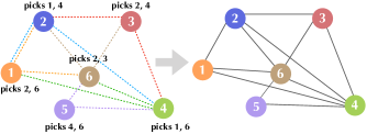
Figure 1: A WSN with $6$ nodes secured by the random pairwise key predistribution scheme with scheme parameter $K=2$. Each node randomly selects $K=2$ nodes and unique pairwise cryptographic keys are given to node pairs per selection. Two nodes can communicate securely if they have at least one key in common. This induces a graph with edges corresponding to node pairs that share a key.

In several networked applications, connectivity is a fundamental determinant of the system performance. For instance, connectivity enables any pair of nodes to exchange messages in a communication network, or exchange funds in a cryptocurrency network. However, establishing links can be costly and often the goal is to obtain a connected network as efficiently as possible, i.e., by using the least amount of resources (links). The connectivity of random K-out graphs and their heterogeneous variants have been extensively studied [4, 15, 16, 17]. It is known [15, 4] that random K-out graphs are connected with probability tending to one (as $n\rightarrow\infty$) if and only if $K\geq 2$. In particular, the following zero-one law holds:

$$\lim_{n\to\infty}\mathbb{P}\left[\mathbb{H}(n;K)\text{ is connected}\right]=\begin{cases}1&\mathrm{if}~{}~{}K\geq 2,\\ 0&\mathrm{if}~{}~{}K=1.\end{cases}$$ (1)

A key advantage of $\mathbb{H}(n;K)$ is its ability to get connected very easily. With $K=2$, $\mathbb{H}(n;K)$ contains at most 2n edges meaning that on average, each node has a degree of less than 4. On the other hand, the classical Erdős-Rényi (ER) random graph [18] requires an average degree of the order of $\log n$ for connectivity; other models with similar connectivity behavior to ER graphs include random key graphs [19] and random geometric graphs [20]. Most existing results for random K-out graphs describe the behavior of the network when the number of nodes $n$ approaches $\infty$ in the form of asymptotic zero-one laws. However, in practical scenarios, the number of nodes in the network are often constrained to be finite. This raises the need to go beyond the asymptotic results (valid for $n\rightarrow\infty$) and obtain as tight bounds as possible for the case when $n$ is small.

Let $P(n;K)$ denote the probability of connectivity of $\mathbb{H}(n;K)$ as a function of the number of nodes ($n$) and the number of selections ($K$) per node. Connectivity is a monotonic increasing property in the number of edges and as a consequence $P(n;K)$ increases as $K$ increases. The case where $K=2$ corresponds to the critical threshold (1) for connectivity. Therefore, we first focus on deriving bounds on $P(n;K)$ for the case $K=2$, and then generalize them to all $K\geq 2$. First, we derive the best known lower bound for $P(n;2)$, i.e., the probability of connectivity for $K=2$. Next, by deriving an upper bound on $P(n;2)$, we show that the lower bound matches the upper bound order-wise, implying that further improvement on the order of $n$ is not possible. While our key focus is on the $K=2$ threshold, we also derive the lower and upper bounds for all $K\geq 2$, with our lower bound beating the existing bounds for all $K\geq 2$; see Section III for a detailed comparison of the bounds and the empirical probability of connectivity. Moreover, to the best of our knowledge, our work is the first to derive an upper bound on $P(n;K)$, which shows that the lower bound is order-wise optimal. The matching upper and lower bounds for the general case $K=2$ derived in this paper establish that the probability of connectivity is $1-\Theta({1}/{n^{K^{2}-1}})$, i.e, the probability of not being connected decays as $\Theta({1}/{n^{K^{2}-1}})$. Our results significantly improve the probabilistic guarantees for network designs that induce random K-out graphs. For example, we show that $n=30$ (resp. $n=60$) is sufficient to have a probability of connectivity of $1-10^{-4}$ (resp. $1-10^{-5}$), while the best known previous result would indicate that $n\geq 72$ (resp. $n\geq 150$) is necessary.

Organization: In Section II we describe the random pairwise scheme and the resulting random K-out graphs. In Section III we present our bounds for connectivity in random K-out graphs and compare them with existing results. We present the proofs of the lower and upper bounds, respectively in Sections IV and V, and conclude in Section VI.

Notation: All limits are understood with the number of nodes $n$ going to infinity. While comparing asymptotic behavior of a pair of sequences $\{a_{n}\},\{b_{n}\}$, we use $a_{n}=\mathrm{o}(b_{n})$, $a_{n}=\omega(b_{n})$, $a_{n}=O(b_{n})$, $a_{n}=\Theta(b_{n})$, and $a_{n}=\Omega(b_{n})$ with their meaning in the standard Landau notation. All random variables are defined on the same probability triple $(\Omega,{\mathcal{F}},\mathbb{P})$. Probabilistic statements are made with respect to this probability measure $\mathbb{P}$, and we denote the corresponding expectation operator by $\mathbb{E}$. The cardinality of a discrete set $A$ is denoted by $|A|$ and the set of all positive integers by $\mathbb{N}_{0}$.

II Model: Random K-out Graphs

The random pairwise key predistribution scheme of Chan et al. is parametrized by two positive integers $n$ and $K$ such that $K<n$. This scheme is implemented as follows. Consider a network comprising of $n$ nodes indexed by labels $i=1,2,\dots n$ with unique IDs: ${\rm Id}_{1},\ldots,{\rm Id}_{n}$. Each of the $n$ nodes draws $K$ edges towards $K$ distinct nodes chosen uniformly at random from among all other nodes. Nodes $v_{i}$ and $v_{j}$ are deemed to be paired if at least one of them selected the other; i.e., either $v_{i}$ selects $v_{j}$, or $v_{j}$ selects $v_{i}$, or both. Once the offline pairing process is complete, the set of keys to be inserted to nodes are determined as follows. For any $v_{i},v_{j}$ that are paired with each other as described above, a unique pairwise key $\omega_{ij}$ is generated and inserted in the memory modules of both nodes $v_{i}$ and $v_{j}$ along with the corresponding node IDs. It is important to note that $\omega_{ij}$ is assigned exclusively to nodes $v_{i}$ and $v_{j}$ to be used solely in securing the communication between them. In the post-deployment key-setup phase, nodes first broadcast their IDs to their neighbors following which each node searches for the corresponding IDs in their key rings. Finally, nodes that have been paired verify each others’ identities through a cryptographic handshake [10].

Let $\mathcal{N}:=\{1,2,\dots,n\}$ denote the set of node labels. For each $i\in\mathcal{N}$, let $\Gamma_{n,i}\subseteq\mathcal{N}_{-i}$ denote the labels selected by node $v_{i}$ (uniformly at random from $\mathcal{N}_{-i}$). Specifically, for any subset $A\subseteq{\cal N}_{-i}$, we have

$$\mathbb{P}{[\Gamma_{n,i}=A]}=\left\{\begin{array}[]{cl}{{n-1}\choose{K}}^{-1}&\mbox{if $|A|=K$}\\ 0&\mbox{otherwise.}\end{array}\right.$$ (2)

Thus, the selection of $\Gamma_{n,i}$ is done uniformly amongst all subsets of ${\cal N}_{-i}$ which are of size exactly $K$. Under the full-visibility assumption, i.e., when one-hop secure communication between a pair of sensors hinges solely on them having a common key, a WSN comprising of $n$ sensors secured by the pairwise key predistribution scheme can be modeled by a random K-out graph defined as follows. With $n=2,3,\ldots$ and positive integer $K<n$, we say that two distinct nodes $v_{i}$ and $v_{j}$ are adjacent, denoted by $v_{i}\sim v_{j}$ if they have at least one common key in their respective key rings. More formally,

$$v_{i}\sim v_{j}~{}~{}\quad\mbox{if}~{}~{}~{}\quad j\in\Gamma_{n,i}\vee i\in\Gamma_{n,j}.$$ (3)

Let $\mathbb{H}(n;K)$ denote the undirected random graph on the vertex set $\{v_{1},\ldots,v_{n}\}$ induced by the adjacency notion (3). In the literature on random graphs, $\mathbb{H}(n;K)$ is often referred to as a random $K$-out graph and have been widely studied [5, 4, 21, 15, 22, 23].

III Results and Discussion

In this section, we present our main results, upper and lower bounds for the probability of connectivity of $\mathbb{H}(n;K)$, and compare them with existing results. Throughout, we write

$$P(n;K):=\mathbb{P}[{~{}\mathbb{H}(n;K)~{}\mbox{is connected}~{}}].$$

III-A Main results

We provide our first technical result– an upper bound for the probability of connectivity $P(n;K)$.

Theorem III.1 (Upper Bound)

For any fixed positive integer $K\geq 2$, we have

$$P(n;K)\leq 1-\frac{({K!})^{K}e^{-K(K+1)}}{{K+1}}\cdot\frac{1}{n^{K^{2}-1}}(1+\mathrm{o}(1))$$ (4)

We present the asymptotic version of the upper bound in Theorem III.1 to make it easier to interpret; see Appendix for the more detailed bound with an explicit expression replacing the $(1+o(1))$ term in (4). The dependence of the upper bound on the scheme parameter $K$ can be succinctly captured as follows.

Remark III.2

For a fixed positive integer $K\geq 2$,

$$P(n;K)=1-\Omega\left(\frac{1}{n^{K^{2}-1}}\right).$$ (5)

Given a fixed value of the parameter $K$ ($K\geq 2$), we derive the upper bound on the probability of connectivity by computing the likelihood of existence of isolated components comprising $K+1$ nodes. Due to space constraints, we outline the proof for the case of $K=2$ in Section IV and present the full proof ($K\geq 2$) in the Appendix. In our second main result, we derive an order-wise matching lower bound and show that the probability of connectivity is also $1-O\left(\frac{1}{n^{K^{2}-1}}\right)$.

Theorem III.3 (Lower Bound)

For any fixed positive integer $K\geq 2$, for all $n\geq 4(K+2)$, we have

$$P(n;K)\geq 1-c(n;K)Q(n;K)$$ (6)

where,

$$c(n;K) =\frac{e^{-(K^{2}-1)(1-\frac{K+1}{n})}}{\sqrt{2\pi(K+1)}}\sqrt{\frac{n}{(n-K-1)}},$$ (7)

$$Q(n;K) =\left(\frac{K+1}{n}\right)^{K^{2}-1}+\frac{n}{2}\left(\frac{K+2}{n}\right)^{(K+2)(K-1)}$$ (8)

Remark III.4

For any fixed positive integer $K\geq 2$ we have

$$P(n;K)=1-O\left(\frac{1}{n^{K^{2}-1}}\right).$$ (9)

This shows that our lower bound (6) for connectivity matches our upper bound (4), and is therefore order-wise optimal. Combining (5) and (9), we obtain the following result.

Corollary III.5

For any positive integer $K\geq 2$, for all $n\geq 4(K+2)$, we have

$$P(n;K)=1-\Theta\left(\frac{1}{n^{K^{2}-1}}\right)$$ (10)

The above equation indicates how rapidly $P(n;K)$ converges to one as $n$ grows large.

III-B Previous results in [15, 4]

We present a summary of the related lower bounds [15, 4] on the probability of connectivity. To the best of our knowledge, our work is the first to compute an upper bound on the probability of connectivity for random K-out graphs.

III-B1 Earlier results by Yağan and Makowski [15]

It was established [15, Theorem 1] that for $K\geq 2$,

$$P(n;K)\geq 1-a(K)Q(n;K)$$ (11)

holds for all $n\geq n(K)$ with $n(K)=4(K+2)$, where

$$a(K)=e^{-\frac{1}{2}(K+1)(K-2)}.$$ (12)

III-B2 Earlier results by Fenner and Frieze [4]

A lower bound for probability of connectivity can be inferred from the proof of [4, Theorem 2.1, p. 348]. Upon inspecting Eqn. 2.2 in [4, p. 349] with $p=0$; it can be inferred that

$$P(n;K)\geq 1-b(n;K)Q(n;K)$$ (13)

holds for all $n$ and $K$ such that $K<n$, where

$$b(n;K)=\frac{12n}{12n-1}\sqrt{\frac{1}{2\pi(K+1)}}\sqrt{\frac{n}{n-K-1}}.$$ (14)

Observe from (6), (11) and (13), that the smaller the values of $c(n;K),a(K)$ and $b(n;K)$, the better is the corresponding lower bound. As discussed in [15], the bound (13) by Fenner and Frieze is tighter than (11) when $K=2$, while (11) is tighter than (13) for all $K\geq 3$. Upon examining (7), (12) and (14), we can see that our bound given in Theorem III.1 is tighter than both (11) and (13) for all $K\geq 2$. We illustrate the performance of these bounds in the succeeding discussion.

III-C Discussion

Through simulations, we study how our upper and lower bounds compare with the empirically observed probability of connectivity. We consider a network secured by the pairwise scheme with parameter $K=2$ and compute the empirical probability of connectivity as we vary the number of nodes $n$. For each parameter pair $(n,K)$, we generate $10^{6}$ independent realizations of $\mathbb{H}(n;K)$. To obtain the empirical probability of connectivity, we divide the number of instances for which the generated graph is connected by the total number ($10^{6}$) of instances generated; see Figure 2. Next, we compare the lower bound for $P(n;K)$ presented in Theorem III.3 with the corresponding bounds in [15, 4]. Recall from (1) that $K=2$ is the critical threshold for connectivity of $\mathbb{H}(n;K)$ in the limit of large network size; thus, we focus on the case $K=2$ throughout the simulations. Substituting $K=2$ in (8), (7), (12) and (14), we obtain the following lower bounds on $P(n;2)$,

$$\textrm{YM \cite[cite]{[\@@bibref{}{Yagan2013Pairwise}{}{}]}}:P(n;2)\geq 1-\frac{155}{n^{3}}$$ (15)

$$\textrm{FF \cite[cite]{[\@@bibref{}{FennerFrieze1982}{}{}]}}:P(n;2)\geq 1-\frac{155}{n^{3}}\cdot\frac{12n/(12n-1)}{\sqrt{6\pi}}\sqrt{\frac{n}{n-3}}$$ (16)

$$\textrm{This work}:P(n;2)\geq 1-\frac{155}{n^{3}}\cdot\frac{e^{-(3-\frac{9}{n})}}{\sqrt{6\pi}}\sqrt{\frac{n}{n-3}}$$ (17)

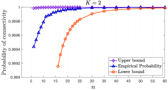
Figure 2: A zoomed in view of our results and empirical probability of connectivity (computed by averaging $10^{6}$ independent experiments for each data point) for $K=2$ as a function of $n$ for $n\geq 16$. The lower bound corresponds to Theorem III.3 and the upper bound corresponds to Theorem III.1.

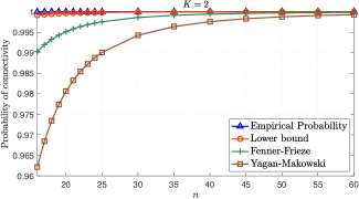
Figure 3: Lower bounds and empirical probability of connectivity (computed by averaging $10^{6}$ independent experiments for each data point) for $K=2$ as a function of $n$ for $n\geq 16$. Our lower bound given in Theorem III.3 significantly improves the existing lower bounds by Yağan and Makowski [15], and Fenner and Frieze [4].

With $K=2$, we plot the lower bounds (6), (11) and (13) for comparison in Figure 3. In Table I, we compare the mean number of realizations of $\mathbb{H}(n;K)$ generated until one disconnected realization is observed corresponding to the lower bounds (15), (16) and (17) for $K=2$.

Our results show that $\mathbb{H}(n;K)$ gets connected with probabilistic guarantees as high as $99.92\%$ even when $K=2$ and network consisting of as few as $16$ nodes. These results complete and complement the existing asymptotic zero-one laws for random K-out graphs.

	Mean number of disconnected realizations
$n$	Theorem III.3	YM [15]	FF [4]
16	1 in 1183	1 in 26	1 in 102
20	1 in 2645	1 in 51	1 in 205
25	1 in 5753	1 in 100	1 in 409
35	1 in 17834	1 in 276	1 in 1145

TABLE I: Comparison of the lower bound (6) with existing lower bounds (11) and (13) from [15] and [4], respectively for $K=2$. The entries in the table corresponds to the mean number of realizations of $\mathbb{H}(n;K)$ generated until one disconnected realization is observed.

IV Upper bound on probability of connectivity

For easier exposition, we give a proof of Theorem III.1 here for $K=2$. Due to space constraints, the general version of our proof for $K\geq 2$ is given in the Appendix. For $K=2$, each node selects at least two other nodes and there can be no isolated nodes or node pairs in $\mathbb{H}(n;K)$. Thus, for $K=2$, the smallest possible isolated component is a triangle, i.e., a complete sub-networks over three nodes such that each node selects the other two nodes. To derive the upper bound on connectivity, we first derive a lower bound on the probability of existence of isolated triangles in $\mathbb{H}(n;K)$. In the proof for the general case $(K\geq 2)$ presented in the Appendix, we investigate the existence of isolated components of size $K+1$.

Let $\Delta_{ijk}$ denote the event that nodes $v_{i},v_{j}$ and $v_{k}$ form an isolated triangle in $\mathbb{H}(n;K)$. The number of isolated triangles in $\mathbb{H}(n;K)$, denoted by $Z_{n}$ is given by

$$Z_{n}=\sum_{1\leq i<j<k\leq n}\mathds{1}\{\Delta_{ijk}\}$$ (18)

Note that the existence of one or more isolated triangles ($Z_{n}\geq 1$), implies that $\mathbb{H}(n;K)$ is not connected. Thus, we can upper bound the probability of connectivity of $\mathbb{H}(n;K)$ as

$$\mathbb{P}[~{}\mathbb{H}(n;K)\text{~{}is connected}~{}]$$

$$=1-\mathbb{P}[~{}\mathbb{H}(n;K)\text{~{}is \emph{not} connected}~{}]$$

$$=1-\mathbb{P}[~{}\exists\text{~{}at least one isolated \emph{sub-network} in~{}}\mathbb{H}(n;K)~{}]$$

$$\leq 1-\mathbb{P}[~{}\exists\text{~{}at least one {isolated} \emph{triangle} in~{}}\mathbb{H}(n;K)~{}]$$

$$=1-\mathbb{P}[~{}Z_{n}\geq 1~{}].$$ (19)

where,

$$\vspace{-1mm}[Z_{n}\geq 1]=\cup_{1\leq i<j<k\leq n}\mathds{1}\{\Delta_{ijk}\}.$$ (20)

In the succeeding discussion, we assume $K=2$ and use the Bonferroni inequality [24] to lower bound the union of the events $\mathds{1}\{\Delta_{ijk}\}$, where $1\leq i<j<k\leq n$.

$$\mathbb{P}[~{}Z_{n}\geq 1~{}]$$

$$\geq\sum_{i<j<k}\mathbb{P}[~{}\Delta_{ijk}~{}]-\sum_{i<j<k}\sum_{x<y<z}\mathbb{P}[~{}\Delta_{ijk}\cap\Delta_{xyz}~{}]$$ (21)

For all $1\leq i<j<k\leq n$ and $1\leq x<y<z\leq n$, we have

$$\mathbb{P}[~{}\Delta_{ijk}~{}]=\left(\frac{{1}}{{n-1\choose 2}}\right)^{3}\left(\frac{{n-4\choose 2}}{{n-1\choose 2}}\right)^{n-3}$$ (22)

Moreover, note that if the sets $\{i,j,k\}$ and $\{x,y,z\}$ have one or more nodes in common, then these sets cannot simultaneously constitute isolated triangles; i.e., the events $\Delta_{ijk}$, $\Delta_{xyz}$ are mutually exclusive if $\{i,j,k\}\cap\{x,y,z\}\neq\emptyset$. Thus,

$$\mathbb{P}[~{}\Delta_{ijk}\cap\Delta_{xyz}~{}]=\begin{cases}&0\text{~{}~{}~{}if~{}}\{i,j,k\}\cap\{x,y,z\}\neq\phi,\\ &\left(\frac{{1}}{{n-1\choose 2}}\right)^{6}\left(\frac{{n-7\choose 2}}{{n-1\choose 2}}\right)^{n-6}\text{otherwise}.\end{cases}$$ (23)

We now calculate the term appearing in (21) in turn. We have

$$\sum_{i<j<k}\mathbb{P}[~{}\Delta_{ijk}~{}] ={n\choose 3}\mathbb{P}[~{}\Delta_{ijk}~{}]$$

$$={n\choose 3}\left(\frac{{1}}{{n-1\choose 2}}\right)^{3}\left(\frac{{n-4\choose 2}}{{n-1\choose 2}}\right)^{n-3}$$

$$=\frac{{4n}}{{3(n-1)^{2}(n-2)^{2}}}\prod_{\ell=1}^{2}\left(1-\frac{3}{n-\ell}\right)^{n-3}$$

$$\geq\frac{{4}}{{3n^{3}}}\left(1-\frac{3}{n-2}\right)^{2n-6},$$ (24)

and

$$\sum_{i<j<k}\sum_{x<y<z}\mathbb{P}[~{}\Delta_{ijk}\cap\Delta_{xyz}~{}]$$

$$={n\choose 3}{n-3\choose 3}\left(\frac{{1}}{{n-1\choose 2}}\right)^{6}\left(\frac{{n-7\choose 2}}{{n-1\choose 2}}\right)^{n-6}$$

$$=\frac{{16n(n-3)(n-4)(n-5)}}{{9(n-1)^{5}(n-2)^{5}}}\prod_{\ell=1}^{2}\left(1-\frac{6}{n-\ell}\right)^{n-6}$$

$$\leq\frac{{16n^{4}}}{{9(n-2)^{10}}}\left(1-\frac{6}{n-1}\right)^{2n-12}.$$ (25)

Substituting (24) and (25) in (21), we obtain

$$\mathbb{P}[~{}Z_{n}\geq 1~{}]$$

$$\geq\sum_{i<j<k}\mathbb{P}[~{}\Delta_{ijk}~{}]-\sum_{i<j<k}\sum_{x<y<z}\mathbb{P}[~{}\Delta_{ijk}\cap\Delta_{xyz}~{}]$$

$$\geq\frac{{4}}{3{n^{3}}}\left(1-\frac{3}{n-2}\right)^{2n-6}-\frac{{16n^{4}}}{{9(n-2)^{10}}}\left(1-\frac{6}{n-1}\right)^{2n-12}$$

$$=\frac{{4e^{-6}}}{3{n^{3}}}(1+\mathrm{o}(1))$$ (26)

Reporting this into (19) leads to establishing Theorem III.1 for $K=2$. More compactly, this result can be stated as $P(n;2)=1-\Omega\left(\frac{1}{n^{3}}\right)$. We prove the more general result for $K\geq 2$ in the Appendix. The next Section is devoted establishing a matching lower bound on the probability of connectivity.

V Lower bound on probability of connectivity

Fix $n=2,3,\ldots$ and consider a fixed positive integer $K$. The conditions

$$2\leq K\quad\mbox{and}\quad e(K+2)<n$$ (27)

are enforced throughout. Note that the condition $e(K+2)<n$ automatically implies $K<n$.

V-A Preliminaries

Before proceeding with the proof, we discuss one of the key steps which distinguishes our proof and improves upon existing[15, 4] bounds. In contrast to the standard bound ${n\choose r}\leq\left(\frac{ne}{r}\right)^{r}$ used in [15], we upper bound ${n\choose r}$ using a variant [25] of Stirling formula. For all $x=1,2,\dots$, we have

$$\sqrt{2\pi}x^{x+0.5}e^{-x}e^{\frac{1}{12x+1}}<x!<\sqrt{2\pi}x^{x+0.5}e^{-x}e^{\frac{1}{12x}},$$ (28)

which gives

$${n\choose{r}} \leq\frac{1}{\sqrt{2\pi}}\left(\frac{n}{n-r}\right)^{n-r}\left(\frac{n}{r}\right)^{r}\frac{\sqrt{n}}{\sqrt{n-r}\sqrt{r}}$$

$$\qquad\cdot\exp\left\{\frac{1}{12n}-\frac{1}{12(n-r)+1}-\frac{1}{12r+1}\right\}$$

$$\leq\frac{1}{\sqrt{2\pi}}\left(\frac{n}{n-r}\right)^{n-r}\left(\frac{n}{r}\right)^{r}\frac{\sqrt{n}}{\sqrt{n-r}\sqrt{r}},$$ (29)

since

$$\frac{1}{12n}-\frac{1}{12(n-r)+1}-\frac{1}{12r+1}<0$$

Using the upper bound for ${n\choose r}$ as presented in (29) eventually leads to the factor $e^{-(K^{2}-1)(1-\frac{K+1}{n})}$ improvement in the lower bound on probability of connectivity in Theorem III.3. Next, we note that for $0\leq K\leq x\leq y$,

$$\frac{{x\choose K}}{{y\choose K}}=\prod_{\ell=0}^{K-1}\left(\frac{x-\ell}{y-\ell}\right)\leq\left(\frac{x}{y}\right)^{K}$$ (30)

since $\frac{x-\ell}{y-\ell}$ decreases as $\ell$ increases from $\ell=0$ to $\ell=K-1$. Lastly, for all $x\in\mathbb{R}$, we have

$$1\pm x \leq e^{\pm x}.$$ (31)

V-B Proof of Theorem III.3

If $\mathbb{H}(n;K)$ is not connected, then there exists a non-empty subset $S$ of nodes that is isolated. Further, since each node is paired with at least $K$ neighbors, $|S|\geq K+1$. Let $C_{n}(K)$ denote the event that $\mathbb{H}(n;K)$ is connected. We have

$$C_{n}(K)^{c}\subseteq\bigcup_{S\in\mathcal{P}_{n}:~{}|S|\geq K+1}~{}B_{n}(K;S)$$ (32)

where $\mathcal{P}_{n}$ stands for the collection of all non-empty subsets of ${\cal N}$. Let $\mathcal{P}_{n,r}$ denotes the collection of all subsets of ${\cal N}$ with exactly $r$ elements. A standard union bound argument yields

$${\mathbb{P}}\left[{C_{n}(K)^{c}}\right] \leq \sum_{S\in\mathcal{P}_{n}:K+1\leq|S|\leq\lfloor\frac{n}{2}\rfloor}{\mathbb{P}}\left[{B_{n}(K;S)}\right]$$ (33)

$$= \sum_{r=K+1}^{\lfloor\frac{n}{2}\rfloor}\left(\sum_{S\in\mathcal{P}_{n,r}}{\mathbb{P}}\left[{B_{n}(K;S)}\right]\right).$$

For each $r=1,\ldots,n$, let $B_{n,r}(K)=B_{n}(K;\{1,\ldots,r\})$. Under the enforced assumptions, exchangeability implies

$${\mathbb{P}}\left[{B_{n}(K;S)}\right]={\mathbb{P}}\left[{B_{n,r}(K)}\right],\quad S\in\mathcal{P}_{n,r}$$

and since $|\mathcal{P}_{n,r}|={n\choose r}$, we have

$$\sum_{S\in\mathcal{P}_{n,r}}{\mathbb{P}}\left[{B_{n}(K;S)}\right]={n\choose r}~{}{\mathbb{P}}\left[{B_{n,r}(K)}\right]$$ (34)

Substituting (34) into (33) we obtain

$${\mathbb{P}}\left[{C_{n}(K)^{c}}\right] \leq\sum_{r=K+1}^{\lfloor\frac{n}{2}\rfloor}{n\choose r}~{}{\mathbb{P}}\left[{B_{n,r}(K)}\right].$$

$$\leq\sum_{r=K+1}^{\lfloor\frac{n}{2}\rfloor}{n\choose r}\left({{r-1}\choose K}\over{{n-1}\choose K}\right)^{r}\left({{n-r-1}\choose K}\over{{n-1}\choose K}\right)^{n-r}.$$ (35)

Using (30) in (35) together with (29), we conclude that

$${\mathbb{P}}\left[{C_{n}(K)^{c}}\right]$$

$$\leq\sum_{r=K+1}^{\lfloor\frac{n}{2}\rfloor}{n\choose r}\left(\frac{r-1}{n-1}\right)^{rK}\left(1-\frac{r}{n-1}\right)^{(n-r)K}$$ (36)

$$\leq\sum_{r=K+1}^{\lfloor\frac{n}{2}\rfloor}{n\choose r}\left(\frac{r}{n}\right)^{rK}\left(1-\frac{r}{n}\right)^{(n-r)K}$$

$$\leq\sum_{r=K+1}^{\lfloor\frac{n}{2}\rfloor}\frac{1}{\sqrt{2\pi}}\left(\frac{n}{n-r}\right)^{n-r}\left(\frac{n}{r}\right)^{r}\frac{\sqrt{n}}{\sqrt{n-r}\sqrt{r}}$$

$$\qquad\cdot\left(\frac{r-1}{n-1}\right)^{rK}\left(1-\frac{r}{n-1}\right)^{(n-r)K}$$

$$=\sum_{r=K+1}^{\lfloor\frac{n}{2}\rfloor}\frac{\sqrt{n}}{\sqrt{2\pi}\sqrt{n-r}\sqrt{r}}\left(\frac{r}{n}\right)^{r(K-1)}\left(1-\frac{r}{n}\right)^{(n-r)(K-1)}$$

$$\leq\sum_{r=K+1}^{\lfloor\frac{n}{2}\rfloor}\frac{\sqrt{n}}{\sqrt{2\pi}\sqrt{n-r}\sqrt{r}}\left(\frac{r}{n}\right)^{r(K-1)}e^{-\left(\frac{r}{n}\right){(n-r)(K-1)}},$$ (37)

where (37) follows from (31). For $K+1\leq r\leq\lfloor\frac{n}{2}\rfloor,$ we have

$$r(n-r)\geq(K+1)(n-K-1)$$ (38)

Substituting in (37),

$${{\mathbb{P}}\left[{C_{n}(K)^{c}}\right]}$$

$$\leq\sum_{r=K+1}^{\lfloor\frac{n}{2}\rfloor}\frac{\sqrt{n}}{\sqrt{2\pi}\sqrt{n-K-1}\sqrt{K+1}}\left(\frac{r}{n}\right)^{r(K-1)}$$

$$\qquad\cdot e^{-\left(\frac{K+1}{n}\right){(n-K-1)(K-1)}}$$

$$=\sum_{r=K+1}^{\lfloor\frac{n}{2}\rfloor}\left(\frac{r}{n}\right)^{r(K-1)}\frac{e^{-(K^{2}-1)(1-\frac{K+1}{n})}}{\sqrt{2\pi(K+1)}}\sqrt{\frac{n}{(n-K-1)}}.$$

$$=c(n;K)\sum_{r=K+1}^{\lfloor\frac{n}{2}\rfloor}\left(\frac{r}{n}\right)^{r(K-1)}$$

$$=c(n;K)\left(\frac{K+1}{n}\right)^{K^{2}-1}+c(n;K)\sum_{r=K+2}^{\lfloor\frac{n}{2}\rfloor}\left(\frac{r}{n}\right)^{r(K-1)}$$ (39)

with $c(n;K)$ given by (7). Due to space constraints we in present the sequence of steps leading to the final bound in Theorem III.3 in the Appendix.

VI Conclusions

In this work we derive upper and lower bounds for connectivity for random K-out graphs when the number of nodes is finite. Our matching upper and lower bounds prove that the probability of connectivity is $1-\Theta({1}/{n^{K^{2}-1}})$ for all $K\geq 2$. Our lower bound is shown to significantly improve the existing ones. In particular, our results further strengthen the applicability of random K-out graphs as an efficient way to construct a connected network topology even when the number of nodes is small. It would be interesting to pursue further applications of K-out graphs in the context of cryptographic payment channel networks.

Appendix

VI-A Upper bound on probability of connectivity for $K\geq 2$

In Section IV we proved Theorem III.1 for the case $K=2$. In this section, we prove the upperbound for the general case $K\geq 2$. Let $K$ be a fixed positive integer such that $K\geq 2$. Let $\Delta_{i_{1}\dots i_{K+1}}$ denote the event that nodes $v_{i},v_{j},\dots,v_{K+1}$ form an isolated component in $\mathbb{H}(n;K)$. The number of such isolated components of size $K+1$ in $\mathbb{H}(n;K)$, denoted by $Z_{n}$ is given by

$$Z_{n}=\sum_{1\leq i_{1}<i_{2}\dots<i_{K+1}\leq n}\mathds{1}\{\Delta_{i_{1}\dots i_{K+1}}\}$$ (40)

Note that the existence of one or more isolated components of size $K+1$ ($Z_{n}\geq 1$), implies that $\mathbb{H}(n;K)$ is not connected. We can upper bound the probability of connectivity of $\mathbb{H}(n;K)$ as

$$\mathbb{P}[~{}\mathbb{H}(n;K)\text{~{}is connected}~{}]$$

$$=1-\mathbb{P}[~{}\mathbb{H}(n;K)\text{~{}is \emph{not} connected}~{}]$$

$$=1-\mathbb{P}[~{}\exists\text{~{}at least one isolated \emph{sub-network}}~{}]$$

$$\leq 1-\mathbb{P}[~{}\exists\text{~{}at least one {isolated} component of size $K+1$}~{}]$$

$$=1-\mathbb{P}[~{}Z_{n}\geq 1~{}].$$ (41)

where,

$$\{Z_{n}\geq 1\}=\bigcup_{1\leq i_{1}<i_{2}\dots<i_{K+1}\leq n}\mathds{1}\{\Delta_{i_{1}\dots i_{K+1}}\}.$$ (42)

In the succeeding discussion, we use the Bonferroni inequality [24] to lower bound the union of the events given in (41).

$$\mathbb{P}[~{}Z_{n}\geq 1~{}]$$

$$\geq\sum_{i_{1}<i_{2}\dots<i_{K+1}}\mathbb{P}[~{}\Delta_{i_{1}\dots i_{K+1}}~{}]$$ (43)

$$\qquad-\sum_{i_{1}<i_{2}\dots<i_{K+1}}\sum_{j_{1}<j_{2}\dots<j_{K+1}}\mathbb{P}[~{}\Delta_{i_{1}\dots i_{K+1}}\cap\Delta_{j_{1}\dots j_{K+1}}~{}]$$ (44)

For all $1\leq i_{1}<i_{2}\dots<i_{K+1}\leq n$ and $1\leq j_{1}<j_{2}\dots<j_{K+1}\leq n$, we have

$$\mathbb{P}[~{}\Delta_{i_{1}\dots i_{K+1}}~{}]=\left(\frac{{1}}{{n-1\choose K}}\right)^{K+1}\left(\frac{{n-K-2\choose K}}{{n-1\choose K}}\right)^{n-K-1}$$ (45)

Moreover, note that if the sets $\{i_{1},\dots,i_{K+1}\}$ and $\{j_{1},\dots,j_{K+1}\}$ have one or more nodes in common, then these sets cannot simultaneously constitute isolated components. Thus, $\mathbb{P}[~{}\Delta_{i_{1}\dots i_{K+1}}\cap\Delta_{j_{1}\dots j_{K+1}}~{}]=$

$$\begin{cases}&0\text{~{}~{}~{}if~{}~{}~{}}\{i_{1},\dots,i_{K+1}\}\cap\{j_{1},\dots,j_{K+1}\}\neq\phi,\\ &\left(\frac{{1}}{{n-1\choose K}}\right)^{2(K+1)}\left(\frac{{n-2K-3\choose K}}{{n-1\choose K}}\right)^{n-2(K+1)}\text{otherwise}.\end{cases}$$ (46)

We now calculate the term appearing in (44) in turn. We have

$$\sum_{i_{1}<i_{2}\dots<i_{K+1}}\mathbb{P}[~{}\Delta_{i_{1}\dots i_{K+1}}~{}]$$

$$={n\choose{K+1}}\mathbb{P}[~{}\Delta_{i_{1}\dots i_{K+1}}~{}]$$

$$={n\choose{K+1}}\left(\frac{{1}}{{n-1\choose K}}\right)^{K+1}\left(\frac{{n-K-2\choose K}}{{n-1\choose K}}\right)^{n-K-1}$$

$$=\frac{({K!})^{K}n}{{K+1}}\cdot\left(\frac{(n-K-1)!}{(n-1)!}\right)^{K}\prod_{\ell=1}^{K}\cdot\left(1-\frac{K+1}{n-\ell}\right)^{n-K-1}$$

$$\geq\frac{({K!})^{K}}{{K+1}}\cdot\frac{1}{n^{(K^{2}-1)}}\prod_{\ell=1}^{K}\cdot\left(1-\frac{K+1}{n-\ell}\right)^{n-K-1}$$

$$\geq\frac{({K!})^{K}}{{K+1}}\cdot\frac{1}{n^{(K^{2}-1)}}\cdot\left(1-\frac{K+1}{n-K}\right)^{K(n-K-1)}$$ (47)

$$=\frac{({K!})^{K}e^{-K(K+1)}}{{K+1}}\cdot\frac{1}{n^{(K^{2}-1)}}(1+\mathrm{o}(1))$$

where (47) is plain from the observation that for all $\ell$ in $1,\dots,K$,

$$1-\frac{K+1}{n-\ell}\geq 1-\frac{K+1}{n-K}.$$

Next,

$$\sum_{i_{1}<\dots<i_{K+1}}\sum_{j_{1}<\dots<j_{K+1}}\mathbb{P}[~{}\Delta_{i_{1},\dots,i_{K+1}}\cap\Delta_{j_{1},\dots,j_{K+1}}~{}]$$

$$={n\choose{K+1}}{n-K-1\choose{K+1}}\left(\frac{{1}}{{n-1\choose K}}\right)^{2(K+1)}$$

$$\qquad\cdot\left(\frac{{n-2K-3\choose K}}{{n-1\choose K}}\right)^{n-2(K+1)}$$

$$\leq{n\choose{K+1}}{n-K-1\choose{K+1}}\left(\frac{{1}}{{n-1\choose K}}\right)^{2(K+1)}$$

$$\qquad\cdot\left(\frac{n-2K-3}{n-1}\right)^{K(n-2(K+1))}$$ (48)

$$=\frac{n!}{(n-2(k+1))!((K+1)!)^{2}}\left(\frac{{K!}}{{n-1\choose K}}\right)^{2(K+1)}$$

$$\qquad\cdot\left(\frac{n-2K-3}{n-1}\right)^{K(n-2(K+1))}$$

$$=\frac{(K!)^{2(K+1)}}{((K+1)!)^{2}}\frac{n(n-1)\dots(n-2K-3)}{(n(n-1)\dots(n-K))^{2(K+1)}}$$

$$\qquad\cdot\left(\frac{n-2K-3}{n-1}\right)^{K(n-2(K+1))}$$

$$\leq\frac{(K!)^{2(K+1)}}{((K+1)!)^{2}}\cdot\frac{n^{2(K+1)}}{(n-K)^{2K(K+1)}}$$

$$\qquad\cdot\left(1-\frac{2(K+1)}{n-1}\right)^{K(n-2(K+1))},$$ (49)

where (48) follows from (30).Substituting (47) and (49) in (44), we obtain

$$\mathbb{P}[~{}Z_{n}\geq 1~{}]$$

$$\geq\sum_{i_{1}<i_{2}\dots<i_{K+1}}\mathbb{P}[~{}\Delta_{i_{1}\dotsi_{K+1}}~{}]$$

$$-\sum_{i_{1}<i_{2}\dots<i_{K+1}}\sum_{j_{1}<j_{2}\dots<j_{K+1}}\mathbb{P}[~{}\Delta_{i_{1}\dotsi_{K+1}}\cap\Delta_{j_{1},\dots,j_{K+1}}~{}]$$

$$\geq\frac{({K!})^{K}}{{K+1}}\cdot\frac{1}{n^{(K^{2}-1)}}\left(1-\frac{K+1}{n-K}\right)^{K(n-K-1)}$$

$$\qquad-\frac{(K!)^{2(K+1)}}{((K+1)!)^{2}}\cdot\frac{n^{2(K+1)}}{(n-K)^{2K(K+1)}}$$

$$\qquad\cdot\left(1-\frac{2(K+1)}{n-1}\right)^{K(n-2(K+1))}$$

$$=\frac{({K!})^{K}e^{-K(K+1)}}{{K+1}}\cdot\frac{1}{n^{(K^{2}-1)}}(1+\mathrm{o}(1))$$ (50)

$$=\Omega\left(\frac{1}{n^{K^{2}-1}}\right).$$

 
In view of (41), we then obtain for $K\geq 2$ that

$$\mathbb{P}[~{}\mathbb{H}(n;K)\text{~{}is connected}~{}]=1-\Omega\left(\frac{1}{n^{K^{2}-1}}\right).$$

VI-B Bounding the sum in (39)

Recall that $K$ is a fixed positive integer $\geq 2$ and under the constraint (27) we have $K+2\leq\lfloor\frac{n}{2}\rfloor$, and therefore the sum in (39) is not empty. Let

$$\left(\frac{x}{n}\right)^{x(K-1)}=e^{(K-1)f_{n}(x)},\quad x\geq 1$$ (51)

with

$$f_{n}(x)=x\log\left(\frac{x}{n}\right)=x\left(\log x-\log n\right).$$

Observe that $r\rightarrow f_{n}(r)$ decreases monotonically on the interval $r=1,\ldots,\lfloor\frac{n}{e}\rfloor$ and increases monotonically thereafter on the interval $r=\lfloor\frac{n}{e}\rfloor+1,\ldots,\lfloor\frac{n}{2}\rfloor$. Therefore,

$$\max\left(f_{n}(r),\ r=K+2,\ldots,\left\lfloor\frac{n}{2}\right\rfloor\right)$$ (52)

$$= \max\left(f_{n}(K+2),f_{n}\left(\left\lfloor\frac{n}{2}\right\rfloor\right)\right).$$

From (27), we have $K+2\leq\lfloor\frac{n}{e}\rfloor$. Next, we show that

$$f_{n}\left(\left\lfloor\frac{n}{2}\right\rfloor\right)\leq f_{n}(K+2)$$ (53)

for all $n$ large enough, say $n\geq n(K)$ for some finite integer $n(K)$ which depends on $K$. (53) is equivalent to

$$\left\lfloor\frac{n}{2}\right\rfloor\log\left(\frac{\left\lfloor\frac{n}{2}\right\rfloor}{n}\right)\leq(K+2)\left(\log(K+2)-\log n\right),$$

a condition can be expressed as

$$n\left(\frac{\left\lfloor\frac{n}{2}\right\rfloor}{n}\right)\log\left(\frac{\left\lfloor\frac{n}{2}\right\rfloor}{n}\right)\leq(K+2)\left(\log(K+2)-\log n\right).$$

The mapping $t\rightarrow t\log t$ is monotone increasing on the interval $(e^{-1},\infty)$. Since $\left\lfloor\frac{n}{2}\right\rfloor\leq\frac{n}{2}$, for the inequality (53) to hold, if suffices to show

$$-\left(\frac{n}{2}\right)\log 2\leq(K+2)\left(\log(K+2)-\log n\right)$$ (54)

for all $n$ satisfying the constraint

$$\frac{1}{e}<\frac{1}{n}\left\lfloor\frac{n}{2}\right\rfloor.$$

It is easy to see that this occurs for all $n>4$, which is in fact automatically guaranteed under (27). Condition (54) can be simplified to yield

$$\log n\leq\left(\frac{\log 2}{2(K+2)}\right)\cdot n+\log(K+2).$$ (55)

It can be verified that (55) holds as an equality for $n=4(K+2)$ and a strict inequality for all $n>4(K+2)$. Setting $n(K)=4(K+2)$ is therefore sufficient for (54) (hence (53)) to hold. Using (51), (52) and (53) we get

$$\max\left(\left(\frac{r}{n}\right)^{r(K-1)}:\ r=K+2,\ldots,\left\lfloor\frac{n}{2}\right\rfloor\right)$$

$$= \left(\frac{K+2}{n}\right)^{(K+2)(K-1)}\hskip 28.45274pt$$

for all $n\geq n(K)$ yielding

$$\sum_{r=K+2}^{\lfloor\frac{n}{2}\rfloor}\left(\frac{r}{n}\right)^{r(K-1)}\leq\left\lfloor\frac{n}{2}\right\rfloor\cdot\left(\frac{K+2}{n}\right)^{(K+2)(K-1)}.$$

Substituting in (39) and noting that $P(n;K)=1-{\mathbb{P}}\left[{C_{n}(K)^{c}}\right]$, we obtain (6.

References

- [1] S. Boccaletti, V. Latora, Y. Moreno, M. Chavez, and D.-U. Hwang, “Complex networks: Structure and dynamics,” Physics reports, vol. 424, no. 4-5, pp. 175–308, 2006.
- [2] A. Goldenberg, A. X. Zheng, S. E. Fienberg, E. M. Airoldi et al., “A survey of statistical network models,” Foundations and Trends in Machine Learning, vol. 2, no. 2, pp. 129–233, 2010.
- [3] M. E. Newman, D. J. Watts, and S. H. Strogatz, “Random graph models of social networks,” Proceedings of the National Academy of Sciences, vol. 99, no. suppl 1, pp. 2566–2572, 2002.
- [4] T. I. Fenner and A. M. Frieze, “On the connectivity of random -orientable graphs and digraphs,” Combinatorica, vol. 2, no. 4, pp. 347–359, Dec 1982.
- [5] B. Bollobás, Random graphs. Cambridge university press, 2001, vol. 73.
- [6] L. Eschenauer and V. D. Gligor, “A key-management scheme for distributed sensor networks,” in Proceedings of the 9th ACM Conference on Computer and Communications Security, ser. CCS ’02. New York, NY, USA: ACM, 2002, pp. 41–47. [Online]. Available: http://doi.acm.org/10.1145/586110.586117
- [7] A. Perrig, J. Stankovic, and D. Wagner, “Security in wireless sensor networks,” Communications of the ACM, vol. 47, no. 6, pp. 53–57, 2004.
- [8] Y. Xiao, V. K. Rayi, B. Sun, X. Du, F. Hu, and M. Galloway, “A survey of key management schemes in wireless sensor networks,” Computer Communications, vol. 30, pp. 2314 – 2341, 2007, special issue on security on wireless ad hoc and sensor networks. [Online]. Available: http://www.sciencedirect.com/science/article/pii/S0140366407001752
- [9] Y. Wang, G. Attebury, and B. Ramamurthy, “A survey of security issues in wireless sensor networks,” IEEE Communications Surveys Tutorials, vol. 8, no. 2, pp. 2–23, Second 2006.
- [10] H. Chan, A. Perrig, and D. Song, “Random key predistribution schemes for sensor networks,” in Proc. of IEEE S&P 2003, 2003.
- [11] V. Sivaraman, S. B. Venkatakrishnan, K. Ruan, P. Negi, L. Yang, R. Mittal, G. Fanti, and M. Alizadeh, “High throughput cryptocurrency routing in payment channel networks,” in 17th USENIX Symposium on Networked Systems Design and Implementation (NSDI 20), 2020, pp. 777–796.
- [12] V. Sivaraman, S. B. Venkatakrishnan, M. Alizadeh, G. Fanti, and P. Viswanath, “Routing cryptocurrency with the spider network,” in Proceedings of the 17th ACM Workshop on Hot Topics in Networks, ser. HotNets ’18. New York, NY, USA: Association for Computing Machinery, 2018, p. 29–35. [Online]. Available: https://doi.org/10.1145/3286062.3286067
- [13] W. Tang, W. Wang, G. Fanti, and S. Oh, “Privacy-utility tradeoffs in routing cryptocurrency over payment channel networks,” Proceedings of Measurement and Analysis of Computing Systems, Article 29, 2020.
- [14] G. Fanti, S. B. Venkatakrishnan, S. Bakshi, B. Denby, S. Bhargava, A. Miller, and P. Viswanath, “Dandelion++: Lightweight cryptocurrency networking with formal anonymity guarantees,” Proc. ACM Meas. Anal. Comput. Syst., vol. 2, no. 2, pp. 29:1–29:35, Jun. 2018.
- [15] O. Yağan and A. M. Makowski, “On the connectivity of sensor networks under random pairwise key predistribution,” IEEE Transactions on Information Theory, vol. 59, no. 9, pp. 5754–5762, Sept 2013.
- [16] R. Eletreby and O. Yağan, “Connectivity of wireless sensor networks secured by the heterogeneous random pairwise key predistribution scheme,” in Proc. of IEEE CDC 2018, Dec 2018.
- [17] M. Sood and O. Yağan, “Towards k-connectivity in heterogeneous sensor networks under pairwise key predistribution,” in 2019 IEEE Global Communications Conference (GLOBECOM), Dec 2019, pp. 1–6.
- [18] P. Erdős and A. Rényi, “On the strength of connectedness of random graphs,” Acta Math. Acad. Sci. Hungar, pp. 261–267, 1961.
- [19] O. Yağan and A. M. Makowski, “Zero–one laws for connectivity in random key graphs,” IEEE Transactions on Information Theory, vol. 58, no. 5, pp. 2983–2999, 2012.
- [20] M. D. Penrose, Random Geometric Graphs. Oxford University Press, Jul. 2003.
- [21] T. K. Philips, D. F. Towsley, and J. K. Wolf, “On the diameter of a class of random graphs,” IEEE Transactions on Information Theory, vol. 36, no. 2, pp. 285–288, 1990.
- [22] F. Yavuz, J. Zhao, O. Yağan, and V. Gligor, “-connectivity in random -out graphs intersecting erdős-rényi graphs,” IEEE Transactions on Information Theory, vol. 63, no. 3, pp. 1677–1692, 2017.
- [23] O. Yağan and A. M. Makowski, “On the scalability of the random pairwise key predistribution scheme: Gradual deployment and key ring sizes,” Performance Evaluation, vol. 70, no. 7-8, pp. 493–512, 2013.
- [24] J. Galambos, “Bonferroni inequalities,” Ann. Probab., vol. 5, no. 4, pp. 577–581, 08 1977. [Online]. Available: https://doi.org/10.1214/aop/1176995765
- [25] H. Robbins, “A remark on stirling’s formula,” The American mathematical monthly, vol. 62, no. 1, pp. 26–29, 1955.