Hydrodynamical instability with noise in the Keplerian accretion discs: Modified Landau equation

Abstract

Origin of hydrodynamical instability and turbulence in the Keplerian accretion disc as well as similar laboratory shear flows, e.g. plane Couette flow, is a long standing puzzle. These flows are linearly stable. Here we explore the evolution of perturbation in such flows in the presence of an additional force. Such a force, which is expected to be stochastic in nature hence behaving as noise, could be result of thermal fluctuations (however small be), Brownian ratchet, grain-fluid interactions and feedback from outflows in astrophysical discs etc. We essentially establish the evolution of nonlinear perturbation in the presence of Coriolis and external forces, which is modified Landau equation. We show that even in the linear regime, under suitable forcing and Reynolds number, the otherwise least stable perturbation evolves to a very large saturated amplitude, leading to nonlinearity and plausible turbulence. Hence, forcing essentially leads a linear stable mode to unstable. We further show that nonlinear perturbation diverges at a shorter timescale in the presence of force, leading to a fast transition to turbulence. Interestingly, emergence of nonlinearity depends only on the force but not on the initial amplitude of perturbation, unlike original Landau equation based solution.

1 Introduction

Accretion discs are ubiquitous in astrophysics in different forms. Examples are discs formed during birth of planetary systems, discs formed by the mass transfer from a companion object to the central denser object in binary systems, discs around the supermassive black holes at the center of galaxies. However, the process of transfer of matter inward and angular momentum outward is still not well understood due to the inadequate molecular viscosity of matter therein. Hence, to explain the observed luminosity (or temperature) from the disc, we must require other source of viscosity. It is generally believed that the turbulent viscosity helps in transporting angular momentum. Shakura & Sunyaev (1973) and later Lynden-Bell & Pringle (1974) prescribed the origin of turbulent viscosity in accretion discs, but rather in an ad hoc manner. The origin of turbulence was not uncovered then. There are pure hydrodynamical proposals to explain the angular momentum transport in accretion discs, mostly based on stability analysis and further turbulence. Some of these are: transient growth leading to nonlinearity in shear flows (Lominadze et al. 1988; Chagelishvili et al. 2003; Tevzadze et al. 2003; Mukhopadhyay et al. 2005; Afshordi et al. 2005; Shen et al. 2006; Lithwick 2007, 2009), the emergence of Rayleigh-Taylor type instability in the Keplerian flow due to the presence of vertical shear (Nelson et al. 2013; Umurhan et al. 2016; Lin & Youdin 2015; Stoll & Kley 2014, 2016; Barker & Latter 2015), Zombie Vortex instability (Marcus et al. 2013, 2015), convective overstability (Klahr & Hubbard 2014), etc. However they are not free from caveats. Also often they are insufficient to explain transport of angular momentum as inferred from observation, i.e. Shakura-Sunyaev viscosity parameter, $\alpha$ (Shakura & Sunyaev 1973), is quite small to explain the observations. Convective overstability has some saturation, it does not let the perturbation modes to grow indefinitely (Latter 2016).

In the Magnetohydrodynamic (MHD) regime, Balbus & Hawley (1991) found that the turbulence could be through the instability due to the interplay between magnetic field and rotation of the flow, following the idea of Velikhov (1959) and Chandrasekhar (1960). This instability is known as Magneto-Rotational Instability (MRI) and those authors showed that this linear instability in the presence of only weak magnetic field could give rise to MHD turbulence. MRI is extremely successful to explain the origin of turbulence in accretion discs over the years. However, it has some limitation too, particularly in the low ionization regime. Although Salmeron & Wardle (2004, 2005, 2008) argued for the possible existence of MRI in colder accretion flows, particularly in the case of protoplanetary disc, based on ambipolar diffusion, Ohmic diffusion and Hall diffusion, they could not resolve the underlying dead zone problem in the accretion disc completely. Indeed Bai (2013, 2017); Bai & Stone (2013) showed through numerical simulations that due to the nonideal MHD effects, like ambipolar diffusion, Ohmic diffusion and Hall diffusion, MRI gets strongly affected, which pose problem to explain protoplanetary discs. The problem is particularly severe in the low states of cataclysmic variables (Gammie & Menou 1998), the outer part of disc in active galactic nuclei (AGNs) and the underlying dead zone (e.g. Menou 2000; Menou & Quataert 2001), where the ionization is very small such that matter cannot be coupled with the magnetic field, hence MRI gets suppressed. It is, therefore, a general concern of the origin of hydrodynamic turbulence or instability leading to turbulence in these discs.

The limitations of MRI do not end here. Nath & Mukhopadhyay (2015) showed that MRI may be suppressed beyond the Reynolds number ($Re$) $10^{9}$, unless perturbation is tuned appropriately, and at that regime it is the magnetic transient growth which brings nonlinearity and hence plausible turbulence in the system. Note that $Re$ in accretion discs is well above this critical value (Mukhopadhyay 2013). Further, MRI is suppressed in the high resistive limit, while it is relevant only with specifically tuned perturbations in the ideal MHD limit. Also in the ideal inviscid limit (i.e., $Re\rightarrow\infty$), apart from the exponential MRI growth at large times, the flow also undergoes transient growth during finite/dynamical times with comparable or higher growth factors, as demonstrated by Mamatsashvili et al. (2013) (see also, Singh Bhatia & Mukhopadhyay 2016). Apart from this, Pessah & Psaltis (2005) showed that in compressible and differentially rotating flows, axisymmetric MRI gets stabilized beyond a toroidal component of the magnetic field. While their calculations were done in local approximation, Das et al. (2018) confirmed the suppression of MRI in global analysis.

Nevertheless, there is a history of controversy about the stability of Rayleigh stable flows and hence the angular momentum transport via turbulent viscosity in these kind of flows, particularly in accretion discs, in the literature (e.g. Dubrulle et al. 2005a; Dubrulle et al. 2005b; Dauchot & Daviaud 1995; Rüdiger & Zhang 2001; Klahr & Bodenheimer 2003; Richard & Zahn 1999; Kim & Ostriker 2000; Mahajan & Krishan 2008; Yecko 2004a; Mukhopadhyay et al. 2011a; Mukhopadhyay & Chattopadhyay 2013). Efforts have been put forward to resolve this issue in the context of hot accretion discs by considering shearing sheet approximation, with (e.g. Lesur & Longaretti 2005) and without (e.g. Balbus et al. 1996; Hawley et al. 1999) viscosity. Fromang & Papaloizou (2007), based on MHD simulation, argued for the importance of dissipation, both resistive and viscous, in order to conclude angular momentum transport and Pumir (1996) examined sustained turbulence in the presence of Couette typed mean flow but in the absence of rotation. However, by experiment (e.g. Paoletti et al. 2012), simulations in the context of accretion discs (e.g. Avila 2012) and in formation of large objects from the dusty gas surrounding a young star (e.g. Cuzzi 2007; Ormel et al. 2008), transient growth in the case of otherwise linearly stable flows (e.g. Mukhopadhyay et al. 2005; Afshordi et al. 2005; Cantwell et al. 2010; Mukhopadhyay et al. 2011b), people argued for plausible emergence of hydrodynamic instability and hence further turbulence.

The idea of transient amplification (see Schmid et al. 2002, for details) is quite popular to resolve similar issues in laboratory flows. Due to the presence of the large number of active nonnormal modes, the subcritical turbulence has quite rich, strongly nonlinear dynamics (see, e.g., homogeneous shear turbulence in a shearing box-like set up shown by Pumir (1996); Mamatsashvili et al. (2016); Sekimoto et al. (2016)). One of the most important nonlinear processes in this case is the new fundamental cascade process, transverse cascade, which plays a key role in the self-sustaining dynamics of the turbulence. This further ensures regeneration of new transiently growing modes (Mamatsashvili et al. 2016; see also Gogichaishvili et al. 2017, for MHD). However, the Keplerian disc was questioned to have sustained purely hydrodynamic turbulence by this process (e.g., Lesur & Longaretti 2005, also see Mukhopadhyay et al. 2005). Indeed, in direct numerical simulations at $Re\sim 10^{5}$, no sustained turbulence has been found (see, e.g., Lesur & Longaretti 2005; Shen et al. 2006; Shi et al. 2017). Nevertheless, we believe that $Re\sim 10^{5}$ is still quite low for accretion discs to rule out any hydrodynamic turbulence, where the Coriolis force is a strong hindering effect therein to kill emergence of any instability and turbulence. We will demonstrate below that for a low $Re$, the system should have been forced strongly to reveal instability.

We, therefore, search for a hydrodynamical origin of nonlinearity and hence plausible turbulence in the accretion disc.Our emphasis is the conventional linear instability when perturbation grows exponentially, unlike the case of transient growth. We particularly consider here an extra force, to fulfill our purpose. Nath & Mukhopadhyay (2016) initiated the study of hydrodynamics in the presence of an extra force in a simplistic model to observe the growth of perturbations in linear regime in astrophysical as well as in laboratory flows. The examples of the origin of such force in the context of biological sciences are: Brownian ratchets in soft condensed matter and biology (e.g. Ait-Haddou & Herzog 2003; van Oudenaarden & Boxer 1999; Parrondo & Español 1996), fluid-structure interaction in biological fluid dynamics (e.g. Peskin 2002). However, in astrophysical context, particularly in accretion discs, the examples of origin of such force could be: the interaction between the dust grains and fluid parcel in protoplanetary discs (e.g. Henning & Stognienko 1996), back reactions of outflow/jet to accretion discs. These forces are also expected to be stochastic in nature. In fact, much prior to that, Farrell & Ioannou (1993) explored the effect of stochastic force in the linearized Navier-Stokes equations. While it was already known that the maximal growth of threedimensional perturbation far exceeds than that of twodimensional perturbation in channel flows, they wanted to check if stochastic forcing further influences growth of perturbation. However, their exploration was limited to nonrotating flows (or flows without Coriolis effect). Therefore, their results, while suggesting implications to similar astrophysical flows as well, do not prove for it. This is important as astrophysical flows are generally involved with rotation and rotational (Coriolis) effect is prone to kill transient amplification of perturbation (Mukhopadhyay et al. 2005; Afshordi et al. 2005). Recently, the effect of stochastic forcing has been explored in the Keplerian flow (Razdoburdin 2020) and it is shown based on the linear theory only that the zero mean stochastic forcing requires compressible fluid in order to transfer angular momentum in the shearing box approximation. However, the present work differs with respect to that of Razdoburdin (2020) in many aspects and it will be evident as we go along. We explore rigorously the idea put forward by Farrell & Ioannou (1993) and Nath & Mukhopadhyay (2016), even generalizing it with nonlinear effects. Due to the very presence of force (stochastic with nonzero mean or otherwise), we show in the present work that the amplitude of least stable perturbation for a Keplerian flow (and some laboratory flows as well) evolves to lead to nonlinearity and plausible turbulence in the system. This works even in incompressible fluid, but with the nonzero mean of stochastic force or finite (even if very small) effect of the force, if not stochastic, in the flow equations. On the other hand, Razdoburdin (2020) considered multi-mode analysis to investigate transient growth of energy and transfer of angular momentum due to the perturbations in the presence of stochastic force.

The plan of the paper is the following. In §2, we establish the evolution of amplitude of the perturbations in a local disc in the presence of noise acting as an extra force. This is basically modified Landau equation describing nonlinear perturbation, in the presence of the Coriolis and external forces. Note that Landau equation in the context of accretion discs without extra force was explored by Rajesh (2011). In §3, we present the results for perturbation evolution, along with its linear counterpart. By the eigenspectrum analysis in the linear regime, we show how the extra force might affect the flow. We further discuss our results comparing them with the properties of conventional Landau equation (without Coriolis and extra forces) in §4. We also argue therein, how the presence of force effectively changes the sign of growth rate, i.e. the least stable eigenvalue, based on the Landau equation. We conclude in §5 that the presence of force makes the system nonlinear and hence reveals turbulence therein.

2 Landau equation in the presence of an extra force and the Coriolis force

We study the hydrodynamics at a local patch in the accretion disc. We assume the patch to be a cubical box of size $2L$.

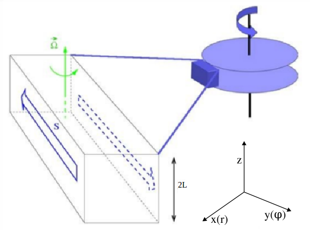
Figure 1: Model picture of local cubical box in accretion disc where we perform the analysis (http://ipag.obs.ujf-grenoble.fr/ longarep/astrophysics.html). Within the box, the Cartesian coordinate $x$ is along the radial cylindrical coordinate $r$ (with respect to the center of the accretion disc), $y$ is along $\phi$, and $z$ is same in both the systems.

The local flow geometry is shown in the Fig. 1, where we use Cartesian coordinates to describe the motion of the local fluid parcel. Usually, cylindrical polar coordinates are used to describe the dynamics of the flow in the accretion disc. However, the directions of the Cartesian coordinates within the box with respect to the cylindrical coordinates are shown in Fig. 1, where the Cartesian coordinates $x,y,z$ are along cylindrical coordinates $r,\phi,z$ respectively. The detailed description of the local formulation can be found in Mukhopadhyay et al. 2005, 2011c. As the fluid is in the local region, we assume the fluid to be incompressible as justified by Yecko (2004b); Mukhopadhyay et al. (2005); Afshordi et al. (2005); Rincon et al. (2007); Nath & Mukhopadhyay (2016). Here we recast the Navier-Stokes equation in Orr-Sommerfeld and Squire equations in the presence of additional stochastic force (Farrell & Ioannou 1993) and Coriolis force, by eliminating the pressure, utilizing the equation of continuity and ensemble averaging (see Nath & Mukhopadhyay 2016), given by

$$\begin{split}\left(\frac{\partial}{\partial t}+U\frac{\partial}{\partial y}\right)\nabla^{2}u-U^{\prime\prime}\frac{\partial u}{\partial y}+\frac{2}{q}\frac{\partial\zeta}{\partial z}\\ -\frac{1}{Re}\nabla^{4}u+\Gamma_{1}=NL^{u},\end{split}$$ (1)

$$\begin{split}\left(\frac{\partial}{\partial t}+U\frac{\partial}{\partial y}\right)\zeta-U^{\prime}\frac{\partial u}{\partial z}-\frac{2}{q}\frac{\partial u}{\partial z}\\ -\frac{1}{Re}\nabla^{2}\zeta+\Gamma_{2}=NL^{\zeta},\end{split}$$ (2)

where $u$ and $\zeta$ are respectively the $x$-component of the velocity and vorticity perturbations after ensemble averaging, $U$ the $y$-component of background velocity which for the present purpose of plane shear in the dimensionless units is $-x$ (see Appendix A), $q$ the rotation parameter with $\Omega(r)\propto 1/r^{q}$, $\Omega(r)$ being the angular frequency of the fluid parcel at radius $r$, $\Gamma$-s are the corresponding constant means of stochastic forces (white noise with nonzero mean due to gravity making the system biased, see Nath & Mukhopadhyay 2016)^, in the system described below and $NL$-s are the non-linear terms of perturbation. As described in Appendix A, in principle in the presence of force, background velocity should be modified with a quadratic variation of $x$ in the $y$-direction. However, depending on the force strength, the $x^{2}$-term may or may not be negligible with respect to the $x$-term. Indeed, for a very small magnitude of this external force, $x^{2}$-term can be neglected keeping background velocity profile same as that without force, as shown explicitly in Appendix A. Also, the detailed derivation of equations (1) and (2) is shown in Appendix B. The $x$-component of vorticity and the non-linear terms are given by

$$\zeta = \frac{\partial w}{\partial y}-\frac{\partial v}{\partial z},$$ (3)

$$NL^{u} = -\nabla^{2}\{(\textbf{u}^{\prime}\cdot\nabla)u\}+\frac{\partial}{\partial x}\nabla\cdot\{(\textbf{u}^{\prime}\cdot\nabla)\textbf{u}^{\prime}\},$$ (4)

$$NL^{\zeta} = -\frac{\partial}{\partial y}\{(\textbf{u}^{\prime}\cdot\nabla)w\}+\frac{\partial}{\partial z}\{(\textbf{u}^{\prime}\cdot\nabla)v\},$$ (5)

where $\textbf{u}^{\prime}=(u,v,w)$, which is the perturbed velocity vector, the derivation of equations (4) and (5) is also shown in Appendix B. However, Farrell & Ioannou (1993) assumed that the perturbation itself is stochastic without considering possible change in background flow due the forcing. They argued that the stochasticity in the dynamical system stems from the random nature of the forcing arisen during perturbation, in our case $\Gamma_{1,2}$, more precisely their properties before ensemble averaging, i.e. $F_{1,2}$ or $F_{x,y,z}$, as shown in Appendix B.

Note that the flow variables, $u$ and $\zeta$, become stochastic variables due to the effect of stochastic force in the flow. Hence, we ensemble average this stochasticity while we derive the temporal dependence of the perturbation in linear and nonlinear regimes. The linearized versions of equations (1) and (2) before ensemble averaging are given in equation (1) in Farrell & Ioannou 1993 and equations (1) and (2) in Nath & Mukhopadhyay 2016 and they also can be obtained from equations (68) and (69) in Appendix B by removing the nonlinear terms. Equations (1) and (2), along with the equation of continuity for incompressible flow given by

$$\nabla\cdot\textbf{u}^{\prime}=0,$$ (6)

form the solvable system of differential equations. We choose the no-slip boundary conditions along $x$ direction (Ellingsen et al. 1970; Yecko 2004b; Mukhopadhyay et al. 2005; Rincon et al. 2007), i.e. $u=v=w=0$ at $x=\pm 1$ or equivalently

$$u=\frac{\partial u}{\partial x}=\zeta=0,\,\ {\rm at}\,\,x=\pm 1.$$ (7)

However, we consider periodic boundary conditions in $y$ and $z$ directions, as the perturbations in these directions can be written in terms of Fourier modes due to the translational invariance of the background flow along these directions. It is well known (e.g. Lin 1961; Butler & Farrell 1992; Mukhopadhyay et al. 2005) that the solutions for the homogeneous part of equations (1) and (2) with nonzero viscosity will form a complete set of discrete eigenmodes. However interestingly note that earlier Mukhopadhyay et al. (2005) and Afshordi et al. (2005) showed the solutions of Orr-Sommerfeld and Squire equations in the context of linear instability in accretion discs practically do not depend on the fact whether $x$ is bounded or extended in infinite domain.

2.1 Plausible source of extra force

We propose two plausible sources for the force in the context of accretion disc. One could be due to the dust-grain in protoplanetary disc interacting with the fluid flow and the other one could be the feedback from jet or outflow onto the accretion disc. These two processes could be modeled considering fluid-particle interactions (Carrillo & Goudon 2006). Let us assume that $f(\textbf{r},\bm{\xi},t)d^{3}\xi$ be the number per unit volume of spherical particles of radius $a$ at position r, having velocity within $\bm{\xi}$ and $\bm{\xi}+d\bm{\xi}$, which may describe the grains floating in the protoplanetary disc. The force, therefore, on a particle by the fluid parcel is $6\pi\mu a(\bm{\xi}-\textbf{U})$, where $\mu$ is the dynamical viscosity and U is the fluid velocity. On the other hand, the force acting on the fluid parcel of unit mass by the particles is $\int_{\bm{\xi}}{6\pi\nu a(\textbf{U}-\bm{\xi})fd\bm{\xi}}$, where $\nu$ is the kinematic viscosity of the fluid of density $\rho$ and is defined by $\mu/\rho$. Now, the number density function $f$ is expected to be stochastic in nature for both the cases in the context of accretion discs due to the stochastic nature of motion of floating dust-grains and feedback, hence the force is. Let us consider the velocity of the particles has radial dependence, i.e. $\xi=\xi(\textbf{r})$. Since the analysis is done in a shearing box at a particular radius with a very small radial width, we assume the number of particles per unit volume within the shearing box be $f(t)\Delta^{3}\xi$. The force acting on the fluid parcel of unit mass by the particles, therefore, is $6\pi\nu a(\textbf{U}-\bm{\xi})f(t)\Delta^{3}\xi$. As described in Appendix B in detail, particularly in equation (58), we can consider the background stochastic force to be $\textbf{F}^{\prime\prime}\cong 6\pi\nu a(\textbf{U}-\bm{\xi})f(t)\Delta^{3}\xi$. If we perturb the flow, U will be replaced by $\textbf{U}+\textbf{u}^{\prime}$ and $\textbf{F}^{\prime\prime}$ will become $6\pi\nu a(\textbf{U}-\bm{\xi})f(t)\Delta^{3}\xi+6\pi\nu a\textbf{u}^{\prime}f(t)\Delta^{3}\xi$. After the background subtraction, the extra force, F, becomes $6\pi\nu a\textbf{u}^{\prime}f(t)\Delta^{3}\xi$, when at a particular radius, $f(t)\Delta^{3}\xi$ appears to be independent of spatial coordinates. According to Farrell & Ioannou (1993) however, any forcing arises due to perturbation only. Hence, there is no change of background velocity and above force $\textbf{F}=6\pi\nu a\textbf{u}^{\prime}f(t)\Delta^{3}\xi$ directly impacts in the system during perturbation only and any such forcing arises after background subtraction. In either of the cases, as described in Appendix B, particularly in equations (70) and (71), the components of extra force are therefore

$$F_{1} = \mathcal{K}\nabla^{2}u,$$ (8)

$$F_{2} = \mathcal{K}\zeta,$$ (9)

where $\mathcal{K}$ is $6\pi\nu af(t)\Delta^{3}\xi$.

Apparently the extra force is then involved with the solution itself. Hence in principle, in the context of the said model, $F_{1}$ and $F_{2}$ can be combined with the corresponding first term of equations (1) and (2) respectively. Subsequently, depending on $\mathcal{K}$, stability of flow may be influenced compared to the case without forcing. However, due to the very stochastic nature of the force, equations (8) and (9) turn out to be stochastic in nature, hence they have to be ensemble averaged in order to determine the temporal dependence of the perturbation. Nevertheless, unlike other terms in equations (1) and (2), $u$ and $\zeta$ cannot be trivially separated out from $\mathcal{K}$ while ensemble averaging $\mathcal{K}\nabla^{2}u$ and $\mathcal{K}\zeta$. Hence, for the present purpose, we a priori assume them to be $\Gamma_{1}$ and $\Gamma_{2}$. Indeed, for any other force model, e.g. thermal fluctuation in fluid elements (which is quite a common choice in statistical and condensed matter systems), $F_{1}$ and $F_{2}$ could be quite different and need to be modeled separately. Hence, for generic purpose also, $\Gamma_{1}$ and $\Gamma_{2}$ are chosen to be constant a priori for the present purpose. We assume any time-dependences, even if arisen from $u$ and $\zeta$, averaged out due to their association with random number $\mathcal{K}$.

Now for micrometer size grains and width of shearing box of $0.1$ Schwarzschild radius, around a $m$ solar mass central object $\mathcal{K}\sim 2\times 10^{6}\times m^{2}f^{\prime}(t)\Delta^{3}\xi^{\prime}/Re$, where quantities with “prime" denote their dimensionful values. Obviously, larger $Re$ corresponds to smaller force, which is at per expectation. Similar scaling is true for laboratory flows. For a protoplanetary disc around a 10 solar mass central object with number density of grain $\sim 10^{11}$ cm^-3 (when a typical midplane total number density $\sim 10^{13}$ cm^-3), $\mathcal{K}\sim 2\times 10^{5}$ for $Re\sim 10^{14}$ (see, e.g., Mukhopadhyay 2013, for bounds on disc $Re$).

Had the force not been stochastic in nature or flow variables been separated out from $\mathcal{K}$ even after ensemble averaging, then a linear stability analysis could be performed for the linearized set of equations (1) and (2) in the same spirit of, e.g., Mukhopadhyay et al. (2005) except with modified coefficients of $\nabla^{2}u$ and $\zeta$. This effect has been explored in §3 with examples.

Such forcing has already been demonstrated in biological systems with incompressible fluid (Peskin 2002). Apart from this, Ioannou & Kakouris (2001) mentioned that stochastic forcing in the context of accretion discs could be due to nonlinear terms which are otherwise neglected because of linearisation or due to external processes such as tidal interaction in binaries, outbursts in binary systems, or perturbation debris from shock waves. Note that very tiny thermal fluctuation in fluids may lead to stochastic motion, however small be, of particles. See Appendix B for survival of such force after ensemble averaging. See also Nath & Mukhopadhyay (2016) and references therein, describing other plausible origin of force.

2.2 Linear Theory

In the evolution of linear perturbation, let the linear solutions be

$$u=\hat{u}(x,t)e^{i\textbf{k}\cdot\textbf{r}},$$ (10)

$$\zeta=\hat{\zeta}(x,t)e^{i\textbf{k}\cdot\textbf{r}},$$ (11)

with $\textbf{k}=(0,k_{y},k_{z})\ {\rm and}\ \textbf{r}=(0,y,z).$ Substitute these in equations (1) and (2), neglecting non-linear terms, we obtain

$$\begin{split}(\mathcal{D}^{2}-k^{2})\frac{\partial\hat{u}}{\partial t}+ik_{y}U(\mathcal{D}^{2}-k^{2})\hat{u}-U^{\prime\prime}ik_{y}\hat{u}+\frac{2}{q}ik_{z}\hat{\zeta}\\ -\frac{1}{Re}(\mathcal{D}^{2}-k^{2})^{2}\hat{u}+\Gamma_{1}e^{-i\textbf{k}\cdot\textbf{r}}=0\end{split}$$ (12)

and

$$\begin{split}\frac{\partial\hat{\zeta}}{\partial t}+ik_{y}U\hat{\zeta}-\left(U^{\prime}+\frac{2}{q}\right)ik_{z}\hat{u}-\frac{1}{Re}(\mathcal{D}^{2}-k^{2})\hat{\zeta}\\ +\Gamma_{2}e^{-i\textbf{k}\cdot\textbf{r}}=0,\end{split}$$ (13)

where $\mathcal{D}=\frac{\partial}{\partial x}$. Recasting equation (12) we obtain

$$\begin{split}\frac{\partial\hat{u}}{\partial t}+i(\mathcal{D}^{2}-k^{2})^{-1}\Bigl{[}k_{y}U\left(\mathcal{D}^{2}-k^{2}\right)-k_{y}U^{\prime\prime}\\ -\frac{1}{iRe}(\mathcal{D}^{2}-k^{2})^{2}\Bigr{]}\hat{u}+(\mathcal{D}^{2}-k^{2})^{-1}\frac{2}{q}ik_{z}\hat{\zeta}\\ +(\mathcal{D}^{2}-k^{2})^{-1}\Gamma_{1}e^{-i\textbf{k}\cdot\textbf{r}}=0.\end{split}$$ (14)

Further combining equations (14) and (13) we obtain

$$\begin{split}\frac{\partial}{\partial t}Q+i\mathcal{L}Q+\Gamma=0,\end{split}$$ (15)

where

$$\begin{split}Q=\begin{pmatrix}\hat{u}\\ \hat{\zeta}\end{pmatrix},\ \mathcal{L}=\begin{pmatrix}\mathcal{L}_{11}&\mathcal{L}_{12}\\ \mathcal{L}_{21}&\mathcal{L}_{22}\end{pmatrix},\end{split}$$ (16)

$$\begin{split}\mathcal{L}_{11}=&(\mathcal{D}^{2}-k^{2})^{-1}\Bigl{[}k_{y}U\left(\mathcal{D}^{2}-k^{2}\right)-k_{y}U^{\prime\prime}\\ &-\frac{1}{iRe}\left(\mathcal{D}^{2}-k^{2}\right)^{2}\Bigr{]},\\ \mathcal{L}_{12}=&\left(\mathcal{D}^{2}-k^{2}\right)^{-1}\frac{2k_{z}}{q},\\ \mathcal{L}_{21}=&-\left(U^{\prime}+\frac{2}{q}\right)k_{z},\\ \mathcal{L}_{22}=&k_{y}U-\frac{1}{iRe}\left(\mathcal{D}^{2}-k^{2}\right),\end{split}$$

and

$$\Gamma=e^{-i\textbf{k}\cdot\textbf{r}}\begin{pmatrix}(\mathcal{D}^{2}-k^{2})^{-1}\Gamma_{1}\\ \Gamma_{2}\end{pmatrix}.$$ (17)

Let us subsequently assume the trial solution of equation (15) be

$$Q=AQ_{x}e^{-i\sigma t}-\frac{1}{\mathcal{D}_{t}+i\mathcal{L}}\Gamma,$$ (18)

where $\sigma$ is the eigenvalue corresponding to the particular mode and it is complex having real ($\sigma_{r}$) and imaginary ($\sigma_{i}$) parts,

$$Q_{x}=\begin{pmatrix}\phi^{u}(x)\\ \phi^{\zeta}(x)\end{pmatrix}$$ (19)

and $\mathcal{D}_{t}$ stands for ${\partial}/{\partial t}.$ $Q_{x}$ is the eigenfunction corresponding to the homogeneous part of equation (15), i.e. $Q_{x}$ satisfies $\mathcal{L}Q_{x}=\sigma Q_{x}$. The first term of right hand side of equation (18) is due to the homogeneous part of equation (15) and the second term is due to the inhomogeneous part, i.e. the presence of $\Gamma$, of the same equation. Hence, $Q$ is influenced by the force $\Gamma$.

2.3 Non-linear theory

For the non-linear solution, following similar work but in the absence of force, e.g. Ellingsen et al. 1970; Schmid & Henningson 2001; Schmid et al. 2002; Rajesh 2011, we assume the series solution for velocity and vorticity, i.e.

$$u=\sum_{n\rightarrow-\infty}^{\infty}u_{n}=\sum_{n\rightarrow-\infty}^{\infty}\bar{u}_{n}(t,x)e^{in(\textbf{k}\cdot\textbf{r}-\sigma_{r}t)},$$ (20)

$$\zeta=\sum_{n\rightarrow-\infty}^{\infty}\zeta_{n}=\sum_{n\rightarrow-\infty}^{\infty}\bar{\zeta}_{n}(t,x)e^{in(\textbf{k}\cdot\textbf{r}-\sigma_{r}t)},$$ (21)

when obviously $\bar{u}_{-n}=\bar{u}^{*}_{n}$ and $\bar{\zeta}_{-n}=\bar{\zeta}^{*}_{n}$. This approach will help in comparing our solutions in accretion discs with the existing literature, without losing any important physics, as will be evident below.

We substitute these in equations (1) and (2) and obtain

$$\begin{split}\sum_{n=-\infty}^{+\infty}\Bigl{[}\Bigl{\{}\left(\mathcal{D}^{2}-n^{2}k^{2}\right)\frac{\partial}{\partial t}-in\sigma_{r}\left(\mathcal{D}^{2}-n^{2}k^{2}\right)\\ +ink_{y}U\left(\mathcal{D}^{2}-n^{2}k^{2}\right)-U^{\prime\prime}ink_{y}\Bigr{\}}\bar{u}_{n}+\frac{2}{q}nik_{z}\bar{\zeta}_{n}\\ -\frac{1}{Re}\left(\mathcal{D}^{2}-n^{2}k^{2}\right)^{2}\bar{u}_{n}\Bigr{]}e^{in(\textbf{k}\cdot\textbf{r}-\sigma_{r}t)}+\Gamma_{1}\\ =NL^{u}_{n}e^{in(\textbf{k}\cdot\textbf{r}-\sigma_{r}t)}\end{split}$$ (22)

and

$$\begin{split}\sum_{n=-\infty}^{+\infty}\Bigl{[}\Bigl{\{}\frac{\partial}{\partial t}-in\sigma_{r}+Uink_{y}-\frac{1}{Re}\left(\mathcal{D}^{2}-n^{2}k^{2}\right)\Bigr{\}}\bar{\zeta}_{n}\\ -\left(U^{\prime}+\frac{2}{q}\right)ink_{z}\bar{u}_{n}\Bigr{]}e^{in(\textbf{k}\cdot\textbf{r}-\sigma_{r}t)}+\Gamma_{2}\\ =NL^{\zeta}_{n}e^{in(\textbf{k}\cdot\textbf{r}-\sigma_{r}t)}.\end{split}$$ (23)

Now, we collect the coefficients of the term $e^{i(\textbf{k}\cdot\textbf{r}-\sigma_{r}t)}$, to capture least nonlinear effect following, e.g., Ellingsen et al. (1970); Rajesh (2011), from both sides and obtain

$$\begin{split}\frac{\partial\bar{u}_{1}}{\partial t}-i\sigma_{r}\bar{u}_{1}+i\Bigl{[}\left(\mathcal{D}^{2}-k^{2}\right)^{-1}\Bigl{\{}k_{y}U\left(\mathcal{D}^{2}-k^{2}\right)\\ -U^{\prime\prime}k_{y}-\frac{1}{Re}\left(\mathcal{D}^{2}-k^{2}\right)^{2}\Bigr{\}}\Bigr{]}\bar{u}_{1}\\ +\frac{2}{q}ik_{z}\left(\mathcal{D}^{2}-k^{2}\right)^{-1}\bar{\zeta}_{1}=\left(\mathcal{D}^{2}-k^{2}\right)^{-1}NL^{u}_{1}\end{split}$$ (24)

and

$$\begin{split}\frac{\partial\bar{\zeta}_{1}}{\partial t}-i\sigma_{r}\bar{\zeta}_{1}+Uik_{y}\bar{\zeta}_{1}-\frac{1}{Re}\left(\mathcal{D}^{2}-k^{2}\right)\bar{\zeta}_{1}\\ -\left(U^{\prime}+\frac{2}{q}\right)ik_{z}\bar{u}_{1}=NL^{\zeta}_{1}.\end{split}$$ (25)

Note that $NL^{u}_{n}$ and $NL^{\zeta}_{n}$ contain various combinations of $e^{i(\textbf{k}\cdot\textbf{r}-\sigma_{r}t)}$. See Appendix C for details. If we assume further

$$Q_{1}=\begin{pmatrix}\bar{u}_{1}(x,t)\\ \bar{\zeta}_{1}(x,t)\end{pmatrix},$$ (26)

we can combine equations (24) and (25) to obtain

$$\frac{\partial Q_{1}}{\partial t}-i\sigma_{r}Q_{1}+i\mathcal{L}Q_{1}=NL_{1},$$ (27)

where $NL_{1}=\begin{pmatrix}\left(\mathcal{D}^{2}-k^{2}\right)^{-1}NL^{u}_{1}\\ NL^{\zeta}_{1}\end{pmatrix}$. We assume the solution for $Q_{1}$ to be

$$Q_{1}=\sum_{m=1}^{\infty}{A_{t,m}}{Q_{x,m}}-\frac{1}{\mathcal{D}_{t}+i\mathcal{L}}\Gamma,$$ (28)

where $m$ stands for various eigenmodes.

However, to the first approximation, our interest is in the least stable mode. See Ellingsen et al. 1970 for similar description in two dimensions without $\Gamma$ and Rajesh 2011 for three dimensional Keplerian disc without $\Gamma$. We, therefore, omit the summation and subscript $m$ in equation (28) and obtain

$$Q_{1}={A_{t}}{Q_{x}}-\frac{1}{\mathcal{D}_{t}+i\mathcal{L}}\Gamma.$$ (29)

We then substitute equation (29) in equation (27) and obtain

$$\begin{split}&Q_{x}\frac{dA_{t}}{dt}-\frac{\partial}{\partial t}\Bigl{(}\frac{1}{\mathcal{D}_{t}+i\mathcal{L}}\Bigr{)}\Gamma-i\sigma_{r}A_{t}Q_{x}&\\ &+i\sigma_{r}\Bigl{(}\frac{1}{\mathcal{D}_{t}+i\mathcal{L}}\Bigl{)}\Gamma+iA_{t}\mathcal{L}Q_{x}-i\mathcal{L}\Bigl{(}\frac{1}{\mathcal{D}_{t}+i\mathcal{L}}\Bigl{)}\Gamma&=NL_{1}\end{split}$$

$$\begin{split}\Rightarrow&Q_{x}\frac{dA_{t}}{dt}-(\mathcal{D}_{t}+i\mathcal{L})\Bigl{(}\frac{1}{\mathcal{D}_{t}+i\mathcal{L}}\Bigr{)}\Gamma+A_{t}\underbrace{(-i\sigma Q_{x}+i\mathcal{L}Q_{x})}_{\text{$0$}}&\\ &-\sigma_{i}A_{t}Q_{x}+i\sigma_{r}\Bigl{(}\frac{1}{\mathcal{D}_{t}+i\mathcal{L}}\Bigr{)}\Gamma=|A_{t}|^{2}A_{t}\mathcal{S}&\end{split}$$

$$\begin{split}\Rightarrow Q_{x}\frac{dA_{t}}{dt}-\sigma_{i}A_{t}Q_{x}\underbrace{-\Gamma+i\sigma_{r}\Bigl{(}\frac{1}{\mathcal{D}_{t}+i\mathcal{L}}\Bigr{)}\Gamma}_{\text{$\Gamma^{\prime}$}}=|A_{t}|^{2}A_{t}\mathcal{S}\end{split}$$

$$\Rightarrow Q_{x}\frac{dA_{t}}{dt}-\sigma_{i}A_{t}Q_{x}+\Gamma^{\prime}=|A_{t}|^{2}A_{t}\mathcal{S},$$ (30)

where the detailed calculation for $\Gamma^{\prime}$ is shown in the Appendix D. $\mathcal{S}$ is the spatial contribution from nonlinear term, computed following Rajesh (2011) where our notation $\mathcal{S}$ is represented as $\begin{pmatrix}\mathcal{S}u\\ \mathcal{S}\zeta\end{pmatrix}$. Please note the section 2.4.1, Appendix B and Appendix C of Rajesh (2011) to have the details of $\mathcal{S}$. To obtain $\mathcal{S}$ using separation of variables and for sufficiently small and slowly varying amplitude, we assume the following:

1. $A_{t}$ is so small that $\dot{A_{t}}/A_{t}$ is approximately $\sigma_{i}$.

2. $\frac{\partial}{\partial x}\Bigl{(}\frac{1}{\mathcal{D}_{t}+i\mathcal{L}}\Bigr{)}\Gamma$ is negligible compared to $\frac{\partial}{\partial t}\Bigl{(}\frac{1}{\mathcal{D}_{t}+i\mathcal{L}}\Bigr{)}\Gamma$ as $||\mathcal{D}_{t}^{2}||>||\mathcal{L}^{2}||.$

This is similar to what was considered by Ellingsen et al. (1970) and Rajesh (2011). Now we utilize the bi-orthonormality between $Q_{x}$ and its conjugate function $\tilde{Q}_{x}$ and from equation (2.3) we obtain

$$\frac{dA_{t}}{dt}-\sigma_{i}A_{t}+\mathcal{N}=p|A_{t}|^{2}A_{t},$$ (31)

where

$$\mathcal{N}=\int_{-1}^{1}{dx\tilde{Q}_{x}^{\dagger}\Gamma^{\prime}}$$ (32)

and

$$p=\int_{-1}^{1}{dx\tilde{Q}_{x}^{\dagger}\mathcal{S}}.$$ (33)

Again, we recall the expression for $\Gamma^{\prime}$ as

$$\begin{split}\Gamma^{\prime}=&-\Gamma+i\sigma_{r}\Bigl{(}\frac{1}{\mathcal{D}_{t}+i\mathcal{L}}\Bigr{)}\Gamma&\\ &=-\Gamma+i\sigma_{r}(t-i\mathcal{L}t^{2})(1+\mathcal{L}^{2}t^{2})^{-1}\Gamma.&\end{split}$$ (34)

Throughout the paper, $\Gamma$ from equation (17) has been decomposed as $\Gamma\rightarrow\Gamma\begin{pmatrix}1\\ 1\end{pmatrix}$ by adjusting $\Gamma_{1}$ and $\Gamma_{2}$, as they are only the free parameters.

3 Evolution of perturbations

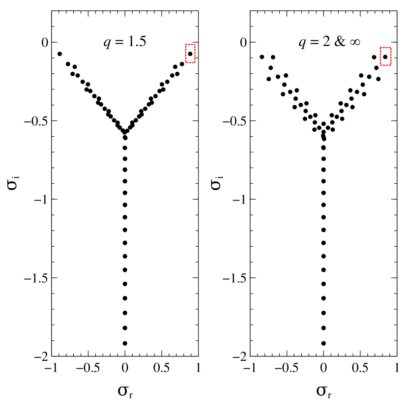
Figure 2: Variation of $\sigma_{i}$ with $\sigma_{r}$ for $Re=2000$ and $k_{y}=k_{z}=1$ for the Keplerian flow ($q=1.5$), constant angular momentum flow ($q=2$) and plane Couette flow ($q\rightarrow\infty$). The latter two eigenspectra are identical. The dotted box represents the least stable mode for the respective cases.

Figure 3: Variation of eigenfunction ($Q_{x}$) for the least stable mode as a function of $x$ for $Re=1000$ and $k_{y}=k_{z}=1$ for the Keplerian flow ($q=1.5$).

We explore here the evolution of the perturbation amplitude based on equation (31). Note, equation (31) is a nonlinear equation. Nevertheless, we explore the results for the linear and nonlinear evolutions both, when for the former, we neglect R.H.S. of equation (31). However, the typical eigenspectra, for linearized Keplerian flow ($q=1.5$), constant angular momentum flow ($q=2$) and plane Couette flow ($q\rightarrow\infty$), for $Re=2000$ and $k_{y}=k_{z}=1$ are shown in the Fig. 2. $\mathcal{L}_{12}$ and $\mathcal{L}_{21}$ in equation (16) are zero for the plane Couette flow and constant angular momentum flow respectively. This is the reason for obtaining same eigenspectra for both plane Couette and constant angular momentum flows. We perform the whole analysis for the least stable modes for the respective flows and these least stable modes are shown in dotted box in Fig. 2. A representative sample eigenvector is displayed in Fig. 3.

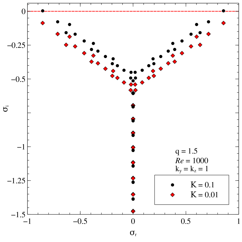
Figure 4: Eigenspectra for the Keplerian flow with $\mathcal{K}=0.1$ and $0.01$, for $Re=1000$ and $k_{y}=k_{z}=1$. Note the uppermost two eigenvalues for $\mathcal{K}=0.1$ with positive $\sigma_{i}$.

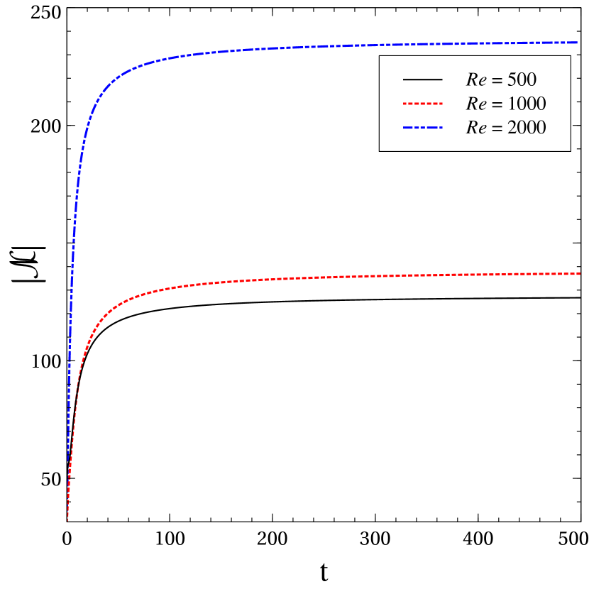
Figure 5: Variation of $\mathcal{N}$ as a function of $t$ for $Re=500,\ 1000$ and 2000, for $\Gamma=10^{4}$ and $k_{y}=k_{z}=1$, corresponding to the respective least stable modes.

As described in §2.1, particularly for equations (8) and (9), if the external force is, e.g., not stochastic in nature, then the effect of force can easily be encoded in the coefficients of $\nabla^{2}u$ and $\zeta$ in equations (1) and (2) respectively, where $\Gamma_{1}=F_{1}$ and $\Gamma_{2}=F_{2}$. Fig. 4 describes the eigenspectra for the Keplerian flow with $Re=1000$ for $\mathcal{K}=0.1$ and $0.01$ for the linearized set of equations (1) and (2) (i.e. $NL^{u}=NL^{\zeta}=0$) and $\Gamma_{1}=F_{1}$ and $\Gamma_{2}=F_{2}$. While $\mathcal{K}=0.1$ makes the flow unstable, $\mathcal{K}=0.01$ cannot. This confirms that depending on external force, $\mathcal{K}$ as defined below equation (9) may in principle destabilize plane shear flows. Now from §2.1, for a 10 solar mass central object, $\mathcal{K}=0.1$, if the floating grains’ number density is of the order of $5\times 10^{-7}$ cm^-3, which is a very small fraction compared to total number density of a protoplanetary accretion disc, hence quite viable. In reality, $Re$ for an accretion disc is several orders of magnitude higher than 1000, hence the required $\mathcal{K}$ for instability could be much smaller (see below for a more concrete description). Nevertheless, in rest of the paper, we concentrate on equations (1) and (2) and their recasting forms without assuming any form of $\Gamma_{1}$ and $\Gamma_{2}$.

3.1 Linear analysis

In the linear regime, equation (31) becomes

$$\frac{dA_{t}}{dt}=\sigma_{i}A_{t}-\mathcal{N}.$$ (35)

From equations (32), (LABEL:eq:exp_for_Gamma') (and also from equation (90)), it is not difficult to understand that at large $t$, $\mathcal{N}$ becomes constant over time, which is depicted in Fig. 5. Now, the solution for equation (35) is

$$A_{t}=-\frac{1}{\mathcal{D}_{t}-\sigma_{i}}\mathcal{N}+Ce^{\sigma_{i}t},$$ (36)

where $C$ is an integration constant and $|A_{t}|$ becomes $|\mathcal{N}|/|\sigma_{i}|$ at large $t$, i.e. when $||\mathcal{D}_{t}||/|\sigma_{i}|<1,$ and $\sigma_{i}$ is negative. The important point here is that the saturation of $|A_{t}|$ does not depend on the initial value of $|A_{t}|$. From wherever we start, $|A_{t}|$ reaches $|\mathcal{N}|/|\sigma_{i}|$ (see below for details).

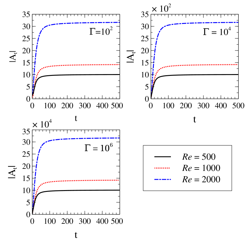
Figure 6: Variation of $|A_{t}|$ as a function of $t$ for three sets of $Re$ and $\Gamma$ with $k_{y}=k_{z}=1$ for linear analysis in the Keplerian flow ($q=1.5$).

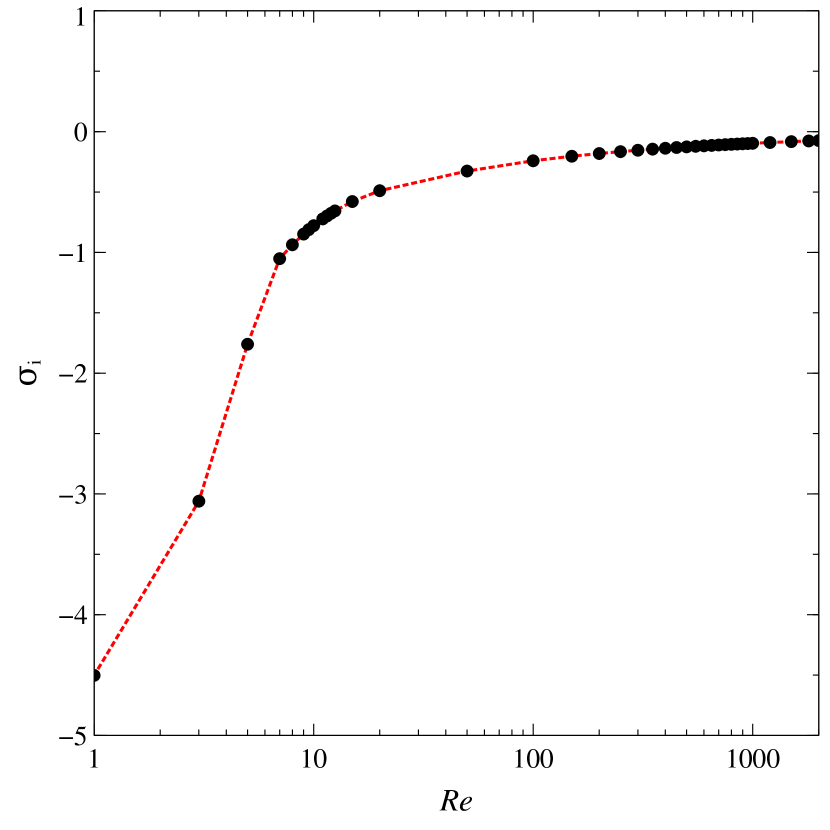
Figure 7: Variation of $\sigma_{i}$ as a function of $Re$ for $k_{y}=k_{z}=1$ in the Keplerian flow.

Fig. 6 shows the variation of $|A_{t}|$ as a function of $t$ for various values of $Re$ and $\Gamma$. From equation (17) we can fix $\Gamma$ by fixing the position, i.e. $x,y$ and $z$, and choosing $\Gamma_{1}$ and $\Gamma_{2}$. Fig. 6 also suggests the scaling relation between saturated $|A_{t}|$ and $\Gamma$ to be

$$|A_{t}|\propto\Gamma$$ (37)

for a fixed $Re$.

Now from Fig. 7, we see that $|\sigma_{i}|$ becomes smaller and smaller as $Re$ increases. On the other hand, Fig. 5 shows that the saturated value of $|\mathcal{N}|$ becomes larger for larger $Re$. Therefore the saturated value of $|A_{t}|$, i.e. $|\mathcal{N}|/|\sigma_{i}|$, becomes larger for larger $Re$. Therefore for $Re=10^{10}$, the saturated value of $|A_{t}|$ will be huge and this in fact leads the perturbations to be highly nonlinear, which further could make the flow turbulent. The emergence of nonlinearity and hence further the turbulence, in this context, can be interpreted in the following way also. At the linear regime, the amplitude $|A_{t}|$ is so small that $|\sigma_{i}A_{t}|\gg|p|A_{t}|^{2}A_{t}|$. If $A_{t}$ evolves in such a way that linear and nonlinear terms become equivalent, i.e. $|A_{t}|^{2}\sim|\sigma_{i}|/|p|$, then the nonlinear part comes into the picture. Now if $Re$ increases, $|\sigma_{i}|$ decreases and $|p|$ increases. Thus, $|A_{t}|$ for the onset of nonlinearity decreases as $Re$ increases. For $Re=500$, $|\sigma_{i}|\sim 10^{-1}$ and $|p|\sim 10^{-4}$ for the Keplerian flow. This leads to $|A_{t}|\sim 33$ for the onset of nonlinearity in the system. From Fig. 6, we notice that for $Re=500$ at $\Gamma=10^{2}$, the saturation value of $|A_{t}|$ is about 8, while at $\Gamma=10^{4}$ the saturated $|A_{t}|$ is about 800. On the other hand, for $Re=2000$, $|\sigma_{i}|\sim 10^{-2}$ and $|p|\sim 10^{-3}$, and the flow starts to become nonlinear at around $|A_{t}|\sim 3.33$ for the Keplerian flow. Fig. 6 suggests that even $\Gamma=10^{2}$ could bring nonlinearity into the system for $Re=2000,$ as the saturation of $|A_{t}|$ therein occurs at around $|A_{t}|\sim 32$ which is almost 10 times the required value of $|A_{t}|$ for onsetting nonlinearity in the system. Hence, with increasing $Re$, required $\Gamma$ to lead to nonlinearity and plausible turbulence becomes smaller and smaller. As $Re$ in accretion discs is quite huge ($\gtrsim 10^{14}$, see, e.g., Mukhopadhyay 2013), required $\Gamma$ is very tiny.

Nevertheless, the occurrence of nonlinearity in this regard is quite amazing. The saturation of $|A_{t}|$ has nothing to do with the initial amplitude of the perturbation. Hence any small disturbance could make the flow nonlinear at a time, having a lower bound: $t>1/|\sigma_{i}|$ (from the assumption $||\mathcal{D}_{t}||/|\sigma_{i}|<1$).

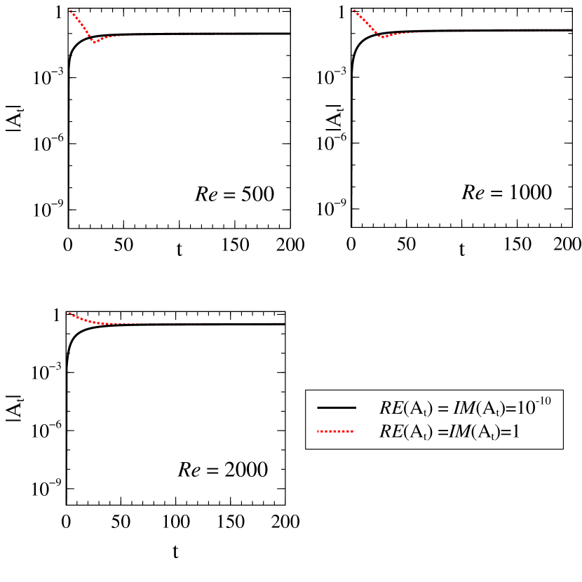
Figure 8: Variation of $|A_{t}|$ as a function of $t$ for $\Gamma=1$ at two different initial conditions with $k_{y}=k_{z}=1$ for three different values of $Re$. The two different initial conditions are real part ($RE(A_{t})$) and imaginary part ($IM(A_{t})$) of $A_{t}$ to be 1 and $10^{-10}$.

Fig. 8 shows the variation of $|A_{t}|$ as a function of $t$ for two initial conditions and for a particular $Re$, showing the same saturated value of $|A_{t}|$. For all three cases $\Gamma$ is 1. This confirms the independence of initial condition.

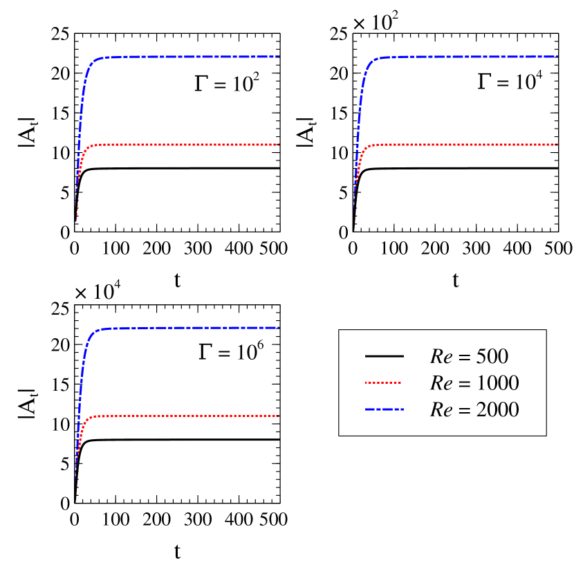
Figure 9: Variation of $|A_{t}|$ as a function of $t$ for three sets of $Re$ and $\Gamma$ with $k_{y}=k_{z}=1$ for the linear analysis in plane Couette flow ($q\rightarrow\infty$).

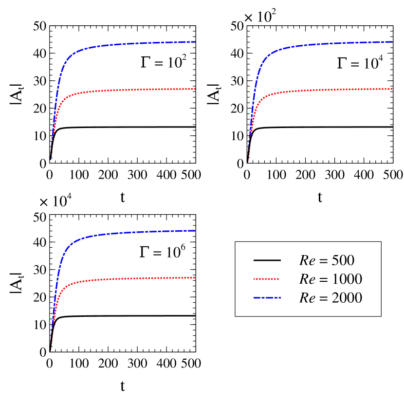
Figure 10: Variation of $|A_{t}|$ as a function of $t$ for three sets of $Re$ and $\Gamma$ with $k_{y}=k_{z}=1$ for the linear analysis in constant angular momentum flow ($q=2$).

Figs. 9 and 10 show the variation of $|A_{t}|$ as a function of $t$ at various $Re$ and $\Gamma$ for plane Couette and constant angular momentum flows. All the results are similar to those of the Keplerian flow. The equation (37) holds for both the cases. But interestingly, the saturated value of $|A_{t}|$ for a particular $Re$ and $\Gamma$ is the largest for constant angular momentum flow and the smallest for plane Couette flow among the three kinds of flow. Although the eigenspectra for constant angular momentum flow and plane Couette flow are same, the eigenmodes corresponding to the same eigenvalues for these two flows are not the same as nonzero matrix elements in $\mathcal{L}$ in equation (16) are not the same for both the flows. Equation (32) shows the dependence of $\mathcal{N}$ on the adjoint eigenmodes of $\mathcal{L}$. This is the reason behind obtaining different evolution of $|A_{t}|$ for the constant angular momentum flow and plane Couette flow. Now we interpret Figs. 6 and 10 in terms of epicyclic frequency which is given by

$$\kappa=\sqrt{2(2-q)}\Omega,$$ (38)

where $\Omega$ is the angular frequency of the fluid parcel. The real value of $\kappa$ indicates the oscillation about the mean position of the fluid parcel, while the imaginary value of $\kappa$ indicates unstable fluid parcel after it is perturbed. However, $\kappa$ is zero for $q=2$ (i.e. constant angular momentum flow) and some positive real number for $q=1.5$ (i.e. the Keplerian flow). Hence, constant angular momentum flow is a marginally stable flow and the Keplerian flow is a well stable flow. From Figs. 6 and 10, we notice that the saturated value of $|A_{t}|$ for constant angular momentum flow is larger than that for the Keplerian flow. The order of nonlinearity is, therefore, higher in the constant angular momentum flow than that in the Keplerian flow and, thence, plausibility of turbulence.

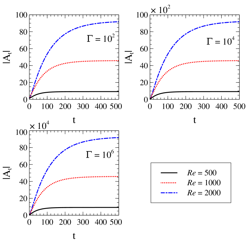
Figure 11: Variation of $|A_{t}|$ as a function of $t$ for three sets of $Re$ and $\Gamma$ with $k_{y}=0.1$ and $k_{z}=1$ for linear analysis in the Keplerian flow.

Fig. 11 shows the variation of $|A_{t}|$ as a function of $t$ at various $Re$ and $\Gamma$ but for $k_{y}=0.1$ and $k_{z}=1$ in the Keplerian flow. This case is a representative example exhibiting vertically dominated perturbation. It also shows that the saturated $|A_{t}|$ is larger compared to that of the $k_{y}=k_{z}=1$ case, when the time to saturate also turns out to be longer. This is due to the fact that $|\sigma_{i}|$ is smaller for this case than that for $k_{y}=k_{z}=1$ case for a fixed $Re$. Similarly, if we make the perturbation more planer, i.e. decrease $k_{z}$ for a fixed $Re$ and $q$, the saturated value of $|A_{t}|$ increases, compared to the $k_{y}=k_{z}=1$ case, but the time to saturate also turns out to be shorter. Fig. 12 depicts this phenomena for the Keplerian flow with $k_{y}=1$ and $k_{z}=0.1$. If we make $k_{z}=0$, the perturbations are entirely two-dimensional and the rotational effect is completely suppressed. The variation of $|A_{t}|$, therefore, will no longer depend on $q$. Fig. 13 shows the variation of $|A_{t}|$ as a function of $t$ for various $Re$ and $\Gamma$ for two-dimensional perturbation, i.e. $k_{y}=1$ and $k_{z}=0$, when the time to saturate is shortest. Note importantly that for each $q$, there is an optimum set of $k_{y}$ and $k_{z}$, giving rise to the best least stable mode and growth, whose imaginary part of eigenvalue decreases with decreasing $q$ below $2$. However, at present, we do not concentrate on the optimum set(s) of $k_{y}$ and $k_{z}$. Hence, stabilizing effect with respect to rotation is not reflected here. Nevertheless, it is evident that as the perturbation varies from vertical to planner, the time to saturate the growth becomes shorter.

Figure 12: Variation of $|A_{t}|$ as a function of $t$ for various $Re$ and $\Gamma$ with $k_{y}=1$ and $k_{z}=0.1$ for linear analysis in the Keplerian flow.

Figure 13: Variation of $|A_{t}|$ as a function of $t$ for various $Re$ and $\Gamma$ with $k_{y}=1$ and $k_{z}=0$ for linear analysis.

3.2 Nonlinear analysis

If there is no extra force involved in the system, then equation (31) becomes the usual Landau equation, which is

$$\frac{dA_{t}}{dt}=\sigma_{i}A_{t}+p|A_{t}|^{2}A_{t},$$ (39)

which can be further recast to

$$\frac{d|A|^{2}}{dt}=k_{1}|A|^{2}+k_{2}|A|^{4},$$ (40)

where $A$ is the amplitude of the nonlinear perturbations for the corresponding system, $k_{1}$ is 2$\sigma_{i}$ and $k_{2}$ is the real part of $2p$, i.e. 2$p_{r}$. Its solution is

$$|A|^{2}=\frac{A_{0}^{2}}{-\frac{k_{2}}{k_{1}}A_{0}^{2}+\left(1+\frac{k_{2}}{k_{1}}A_{0}^{2}\right)e^{-k_{1}t}}.$$ (41)

If both $k_{1}$ and $k_{2}$ are positive, then we can find a particular time (by making the denominator of equation (41) to 0),

$$t=-\frac{1}{k_{1}}ln\left(\frac{k_{2}A_{0}^{2}}{k_{1}+k_{2}A_{0}^{2}}\right)$$ (42)

at which $|A|$ diverges. Therefore, in this case, the system becomes highly nonlinear and we have to consider all kinds of nonlinear effects. Thus the system is expected to become turbulent rapidly.

However, the presence of extra force makes it very difficult for us to have a compact analytical solution like equation (41). Therefore, we venture for numerical solutions of equation (31) for different parameters such as $Re$ and $\Gamma$. Fig. 14 shows the solution of equation (31), describing the variation of $|A_{t}|$ from equation (31) as a function of $t$ for $Re=$ 500 and 2000 for different $\Gamma$ in the Keplerian flow. We notice that $\Gamma$ plays an important role. $|A_{t}|$ saturates for $\Gamma=10^{2}$ beyond a certain time. However, as $\Gamma$ increases to $10^{4}$, we see that $|A_{t}|$ diverges for $Re=2000$ at a certain time, but not for $Re=500$. As the strength of the external force, i.e. $\Gamma$, further increases to $10^{6}$, we see that $|A_{t}|$ diverges at a smaller time and even at a smaller $Re$.

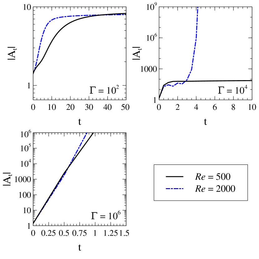
Figure 14: Variation of $|A_{t}|$ as a function of $t$ for different $Re$ and $\Gamma$ with $k_{y}=k_{z}=1$ for nonlinear analysis in the Keplerian flow.

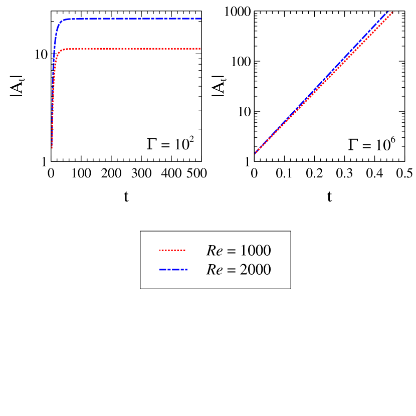
Figure 15: Variation of $|A_{t}|$ as a function of $t$ for different of $Re$ and $\Gamma$ with $k_{y}=k_{z}=1$ for nonlinear analysis in plane Couette flow.

Fig. 15 shows the variation of $|A_{t}|$ as a function of $t$ for different $Re$ for plane Couette flow. The results are quite similar to those for the Keplerian flow.

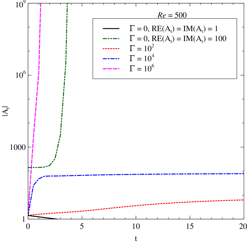
Figure 16: Variation of $|A_{t}|$ as a function of $t$ with $k_{y}=k_{z}=1$ for nonlinear analysis in the Keplerian flow for $Re=500$ and four different $\Gamma$. For $\Gamma\neq 0$, initial condition is RE($A_{t}$) = IM($A_{t}$) = 1.

Nevertheless, in our case, $k_{1}$ in equation (40) is negative. It makes the problem more interesting if $k_{2}>0$. In the absence of force, if the initial amplitude of the perturbation $A_{0}$ is larger than the threshold amplitude,

$$|A|=A_{i}=\sqrt{\frac{-k_{1}}{k_{2}}},$$ (43)

then it is well-known that (see, e.g., Ellingsen et al. 1970; Drazin & Reid 2004 for plane Couette flow, Rajesh 2011 for the Keplerian discs) there will be a time $t$, as given in equation (42) (with suitable sign of $k_{1}$ and $k_{2}$ in mind), at which the solution diverges. This is shown in the Fig. 16 with a dashed-short-dashed (green) growing line starting from finite $|A_{t}|$ for $Re=500$ and $k_{y}=k_{z}=1$, whereas the solid (black) fast decaying line indicates the result with smaller $A_{0}$. Other three curves, starting from the same smaller $|A_{t}|=|A_{0}|$, are showing the variation of $|A_{t}|$ as a function of $t$ in the very presence of the extra force. The pattern of turbulence during its onset in the absence of extra force but with a finite initial amplitude of perturbation at $325\lesssim Re\lesssim 380$ for plane Couette flow was simulated by Duguet et al. (2010). In our case shown in Fig. 16 by the dashed-short-dashed (green) line, we also see the diverging nature of amplitude of the nonlinear perturbation beyond a certain time in the absence of extra force, but in the presence of Coriolis force (which is a stabilizing effect), only with finite initial amplitude of perturbation. This implies the turbulent nature of the flow. It is apparent that the onset of the nonlinearity depends on the initial amplitude of perturbation in the absence of the force, but it does not depend on the same in the presence of force. The divergence of $|A_{t}|$ and hence the onset of nonlinearity and plausible turbulence depends only on the strength of the force, as shown by dashed (magenta) line, compared to dot-dashed (blue) and dotted (red) lines, in Fig. 16. The presence of $\Gamma$ with negative $k_{1}$ ($\sigma_{i}$) is equivalent to the Landau equation and solution with $\Gamma=0$ and $k_{1}$ and $k_{2}$ both positive. With a suitable strength of force, $|A_{t}|$ diverges quicker than that without force.

3.2.1 Plane Couette flow and bounds on parameters

Similar results as above are obtained for plane Couette flow, in accordance with the simulation by Duguet et al. (2010). Fig. 17 shows that for a given initial amplitude of perturbation, while $|A_{t}|$ decays with time for $Re=300$, increasing $Re$ to 370 leads to diverging $|A_{t}|$ at a finite time. Also, for a given $Re$, a smaller initial amplitude of perturbation depending on $Re$, makes $|A_{t}|$ decaying with time. While a very large initial amplitude might make $|A_{t}|$ diverging even at $Re=300$, that situation might be naturally implausible or equivalent to external forcing. That is perhaps the reason that Duguet et al. (2010) found plane Couette flow laminar for $Re<324$. If $|A_{t}|$ should be finite for $Re<324$, initial amplitude should have an upper bound, e.g. $\lesssim 80$, perhaps larger initial amplitude is naturally implausible.

The situation however changes in the presence of force. Fig. 18 shows that for a small initial amplitude of perturbation, only larger $\Gamma$ makes $|A_{t}|$ diverging leading to turbulence. In fact, in the absence of force, $|A_{t}|$ decays with time very fast for the range of $Re$ which however could lead to turbulence at higher initial amplitude of perturbation with $Re>324$ shown by Duguet et al. (2010) in their simulation in the absence of force. In fact Duguet et al. (2010) argued the initial amplitude of perturbation to be sufficiently large to trigger transition to turbulence at $Re$ larger than critical value. However, we can put constraint on the magnitude of $\Gamma$, based on the simulation of Duguet et al. (2010). If $|A_{t}|$ need not diverge at $Re<324$, from Fig. 18 we can argue that $\Gamma$ has to be smaller than $10^{4}$. Perhaps the upper bound of $\Gamma$ may be such that only $Re>324$ will lead to diverging $|A_{t}|$. Keeping this idea in mind, we show in Fig. 19 that for $\Gamma=300$, while $|A_{t}|$ diverges in plane Couette flow hence presumably leading to turbulence for $Re=370$, it saturates without leading to nonlinear regime for $Re=300$. Note that the saturated $|A_{t}|$ is around 30, whereas critical $|A_{t}|$ for nonlinearity to arise is 115.04 for $\Gamma=300$ and $Re=300$. Hence, if the numerical simulation by Duguet et al. (2010) is our guide, then $\Gamma$ for plane Couette flow should be around 300.

Nevertheless, the numerical simulations did not include extra force explicitly. Hence, it need not necessarily mimic exactly what happens in nature. Hence, the above mentioned upper bounds of initial amplitude of perturbation and force should be considered with caution and just as indicative. While by the virtue of direct numerical simulations, they could consider all the modes playing role to reveal turbulence, we have considered extra force in the premise of least stable mode evolution. Hence, both the frameworks appear to be equivalent. Indeed, for the present purpose, we consider magnitude of extra force as a parameter. Hence, an independent simulation and also laboratory experimental results help us to constrain the parameter of the model.

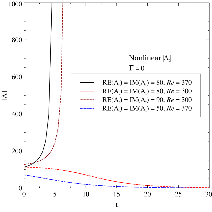
Figure 17: Variation of $|A_{t}|$ as a function of $t$ with $k_{y}=k_{z}=1$ for nonlinear analysis in plane Couette flow without force for different $Re$ and initial conditions.

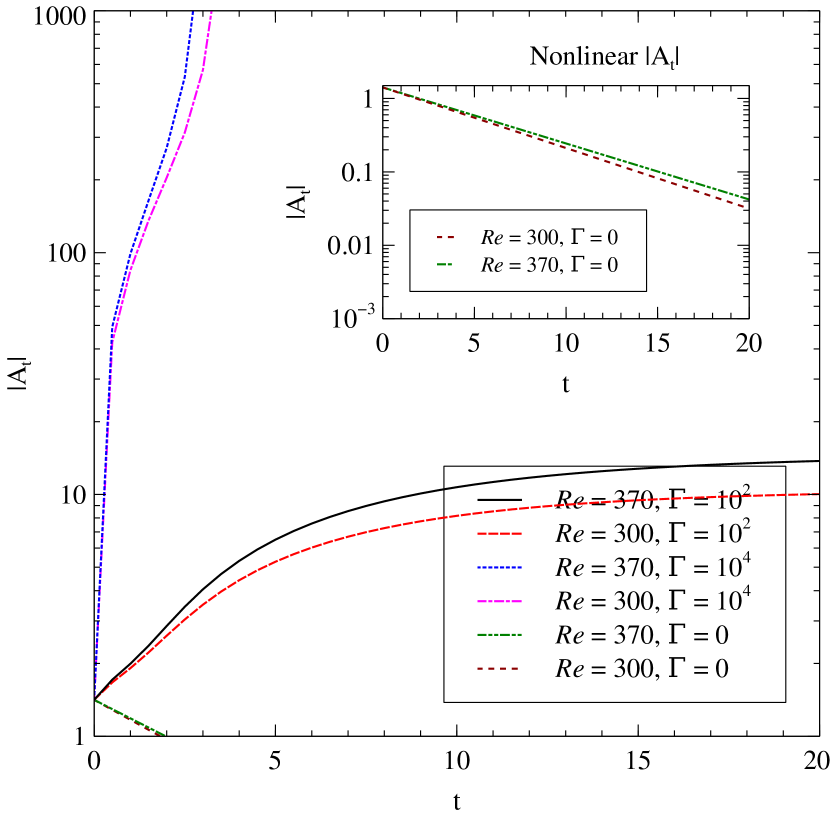
Figure 18: Variation of $|A_{t}|$ as a function of $t$ with $k_{y}=k_{z}=1$ for nonlinear analysis in plane Couette flow for different forces and $Re$ at a fixed initial condition RE($A_{t}$) = IM($A_{t}$) = 1.

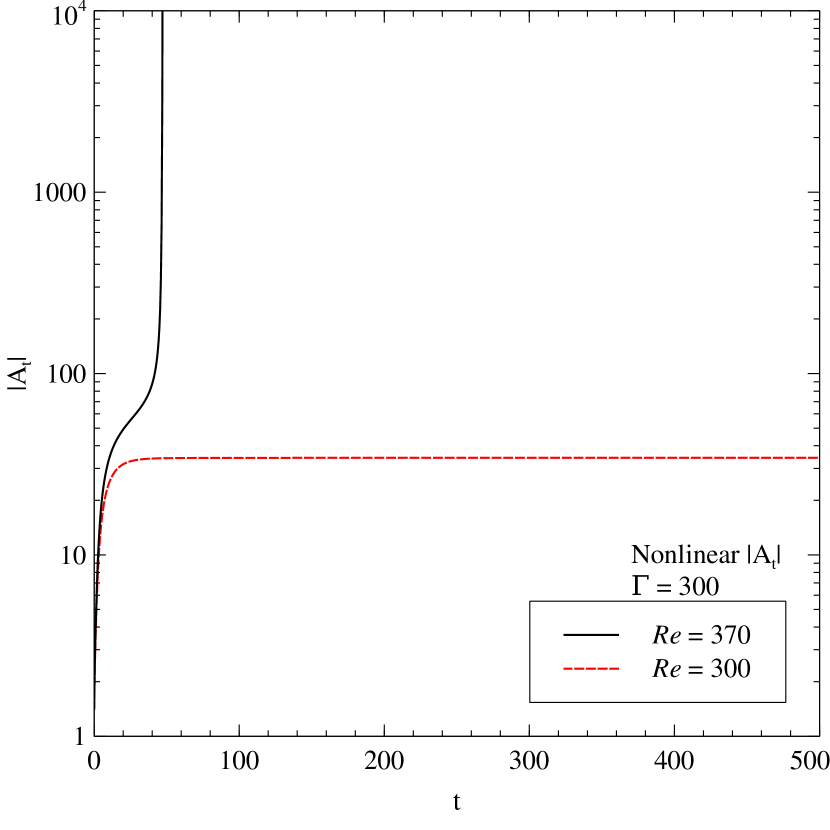
Figure 19: Variation of $|A_{t}|$ as a function of $t$ with $k_{y}=k_{z}=1$ for nonlinear analysis in plane Couette flow for $\Gamma=300$, and $Re=300$ and $370$ at an initial condition RE($A_{t}$) = IM($A_{t}$) = 1.

Above results argue that while $\Gamma$ may have upper bound as expected, large $Re$ requires small $\Gamma$ to trigger instability and turbulence. As accretion disc $Re$ is very large, a small $\Gamma$ would suffice therein.

4 Discussion

Here we compare our results, i.e. the behaviour of the solution of modified Landau equation with force, with the conventional perturbation evolution through the Landau equation without force. The nonlinear evolution of amplitude of perturbations in the absence of extra force (i.e. the usual Landau equation) is given by equation (39) or (40) and the solution is given by equation (41). Depending on the sign (positive/negative) of $k_{1}$ and $k_{2}$, there are four different possible evolutions of $|A|$ (Drazin & Reid 2004; Schmid et al. 2002). In the present context of shear flows, $k_{1}$ (i.e. $\sigma_{i}$) is negative, but $k_{2}$ is positive. Therefore, there will be a threshold for initial amplitude $A_{i}$, as shown in equation (43), determining the growth of perturbation. If the initial amplitude $A_{0}<A_{i}$, then

$$|A|^{2}\sim\frac{A_{i}^{2}A_{0}^{2}e^{k_{1}t}}{A_{i}^{2}-A_{0}^{2}}$$ (44)

at a large $t$. Therefore, $|A|^{2}\rightarrow 0$ for $A_{0}<A_{i}$ at $t\rightarrow\infty$. However, if $A_{0}>A_{i}$, then $|A|^{2}\rightarrow\infty$ at $t\rightarrow\ln(1-A_{i}^{2}/A_{0}^{2})/k_{1}$.

If both $k_{1}$ and $k_{2}$ would be positive, $|A|^{2}$ blows up after a finite time, given by equation (42). Hence, there will be a fast transition to turbulence. On the other hand, if $k_{1}>0$ but $k_{2}<0$, then $|A|^{2}\rightarrow k_{1}/|k_{2}|$ at $t\rightarrow\infty$. In this case, $|A|^{2}$ at a large $t$ does not depend on $A_{0}$. Obviously for $k_{1}$ and $k_{2}$ both negative, $|A|^{2}$ decays fast.

However, we have shown in §3 that the saturation in $|A_{t}|$ is at $|\mathcal{N}|/|\sigma_{i}|$ in the linear regime. We have also shown that the assumption of linear analysis at the saturation of $|A_{t}|$ may no longer be valid depending on $Re$ and $\Gamma$ and, hence, the system may already be in the nonlinear regime. The evolution of $|A_{t}|$ at the linear regime in our case, i.e. with extra force, is similar to that of $|A|$ from equation (40), i.e. without force, for $k_{1}>0$ and $k_{2}<0$. From Figs. 5 and 7, it is obvious that $|\mathcal{N}|$ increases and $|\sigma_{i}|$ decreases with the increment of $Re$. Therefore, at large $Re$ ($\gtrsim 10^{14}$, which is true for accretion discs, see, e.g., Mukhopadhyay 2013), the saturation of $|A_{t}|$ is also large and, hence, at smaller $\Gamma$ also nonlinearity is inevitable fate of the fluid at the local regime of the accretion disc.

In the Keplerian and plane Couette flows, $k_{1}$, i.e. $\sigma_{i}$, is negative, but $k_{2}$, i.e. $p_{r}$, could be positive. In the presence of extra force, Landau equation modifies in such a way that the solution in the linear regime itself mimics the Landau equation without force (i.e. equation 40), however, with $k_{1}>0$ and $k_{2}<0$. Further in the nonlinear regime, the amplitude $A_{t}$ (i.e. with extra force included) diverges beyond a certain time, depending on $Re$ and $\Gamma$. In nonlinear regime, the Landau equation in the presence of extra force but negative $k_{1}$ ($\sigma_{i}$) is, therefore, mimicking the Landau equation without force but with positive $k_{1}$ and $k_{2}$. Essentially, the extra force effectively changes the sign of $k_{1}$ (i.e. $\sigma_{i}$) for the Landau equation without force. Speaking in another way, the very presence of extra force destabilizes the otherwise stable system.

It is important to note that rotational (Coriolis) effect stabilizes the flow (see, e.g., Mukhopadhyay et al. 2005). Hence, for each $q$, there is an optimum set of $k_{y}$ and $k_{z}$, giving rise to the best least stable mode and growth, which (underlying $\sigma_{i}$) decreases with decreasing $q$ below $2$. However, at present, we do not concentrate on this feature and in place of optimum set(s) of $k_{y}$ and $k_{z}$, flows are considered for fixed sets of $k_{y}$ and $k_{z}$. Therefore, stabilizing effect with respect to rotation does not appear here.

5 Conclusion

Origin of hydrodynamical instability and plausible turbulence in Rayleigh stable flows, e.g. the Keplerian accretion disc flow, plane Couette flow, is a long standing problem. While such flows are evident to be turbulent, they are linearly stable for any Reynolds number. Over the years, several attempts are made to resolve the problem, with a very limited success, and often the resolution arises with a caveat. The major success however in this line lies with MRI, hence in the presence of magnetic field. However, several astrophysical and laboratory systems are cold, neutral in charge and unmagnetised. Hence, any instability therein must be hydrodynamical not magnetohydrodynamical.

We show that in the presence of extra force, governed due to, e.g., thermal fluctuation, grain-fluid interactions, the amplitude of perturbation may in fact grow with time. Essentially we have established the Landau equation for nonlinear perturbation in the presence of Coriolis and external forces. Under suitable combination of $Re$ and the external force, perturbation amplitude could be very large. In the linear regime, eventually the amplitude saturates beyond a certain time, but the saturated value could be very large, already leading the system to nonlinear regime, depending on $Re$ (which is basically controlling the value of imaginary part of the eigenvalue of perturbation mode) and the force magnitude. In the nonlinear regime, however, the perturbation amplitude diverges depending on $Re$ and force magnitude. This feature is shown to exist in all the apparently Rayleigh stable flows including accretion discs. Thus, the presence of force plays an important role to develop nonlinearity and turbulence. As argued here and in previous literature (e.g. Nath & Mukhopadhyay 2016), the presence of such force is obvious and hence hydrodynamical instability and turbulence is not to be a big surprise therein. Now it is important to confirm the present findings based on direct numerical simulations, which we plan to undertake in future.

Data availability

No new data were generated or analysed in support of this research.

Appendix A Modification of background flow in the presence of force

Due to the presence of the extra force, the background flow may be modified from its plane Couette flow nature. Let us understand it from a simplistic consideration. Considering the background flow

$$\textbf{V}=(0,V_{Y}(X),0),$$ (45)

the Navier-Stokes equation in the presence of force is

$$\frac{\partial\textbf{V}}{\partial t}+(\textbf{V}\cdot\nabla)\textbf{V}=-\frac{\nabla P}{\rho}+\nu\nabla^{2}\textbf{V}+\bm{F},$$ (46)

where $P$, $\rho$, $\nu$ and F are the pressure, density, kinematic viscosity and extra force, chosen constant for the present purpose, respectively. The three components of equation (46) are

$$0=-\frac{1}{\rho}\frac{\partial P}{\partial X}+F_{X},$$ (47)

$$\begin{split}0=-\frac{1}{\rho}\frac{\partial P}{\partial Y}+\nu\nabla^{2}V_{Y}+F_{Y},\end{split}$$ (48)

$$0=-\frac{1}{\rho}\frac{\partial P}{\partial Z}+F_{Z}.$$ (49)

Equation (48) can be further simplified to

$$\nabla^{2}V_{Y}=\frac{1}{\nu}(-F_{Y}+\frac{1}{\rho}\frac{\partial P}{\partial Y})=\frac{\partial^{2}V_{Y}}{\partial X^{2}}.$$ (50)

Hence, for constant $\partial P/\partial Y$ and $F_{Y}$,

$$\begin{split}V_{Y}=-\left(\frac{F_{Y}}{\nu}-\frac{1}{\nu\rho}\frac{\partial P}{\partial Y}\right)\frac{X^{2}}{2}+C_{1}X+C_{2}&\\ =-K\frac{X^{2}}{2}+C_{1}X+C_{2},\end{split}$$ (51)

where

$$K=\left(\frac{F_{Y}}{\nu}-\frac{1}{\nu\rho}\frac{\partial P}{\partial Y}\right).$$ (52)

The corresponding boundary conditions

$$V_{Y}=\mp U_{0}\ {\rm at}\ X=\pm L$$ (53)

lead $V_{Y}$ in equation (51) to

$$V_{Y}=\frac{K}{2}(L^{2}-X^{2})-\frac{U_{0}X}{L},$$ (54)

where $F_{Y}=\partial P/\partial Y=0$ brings the background back to plane Couette/shear flow. In fact, for ideal plane Couette flow, there is no pressure gradient along any direction. Therefore, $K$ becomes $F_{Y}/\nu$ only and $F_{X}=F_{Z}=0$, assuring the choice of equation (45). In accretion discs, however, $Re$ is very large (and $\nu$ is very small). Hence for a given $K$, a very small $F_{Y}$ suffices. In fact, it has been shown in §3.1 that with the increase of $Re$, $\Gamma$ has to be increasingly small in order to maintain linear approach intact. Therefore, $F_{Y}$ can be smaller than smallness of $\nu$ and therefore the effect of nonlinear term in equation (54) is very small. The flow, therefore, effectively becomes plane Couette flow (or the Keplerian flow in the presence of rotation/Coriolis effect) only. Fig. 20 shows the eigenspectra for the background flow of form $ax+bx^{2}$, where $x=X/L$, the dimensionless length. See Appendix B for all details of the units. This background flow mimics that given by equation (54). However, we observe that the small value of $b/a$ does not affect the eigenspectra much and it almost remains the same as of the Keplerian flow. As small $b/a$ corresponds to small $F_{Y}$, we can assume background flow of linear shear in our model calculations throughout, particularly for high $Re$ flows, e.g. Keplerian flow which is the central essence of the work, where indeed force to be very small (see §3.1).

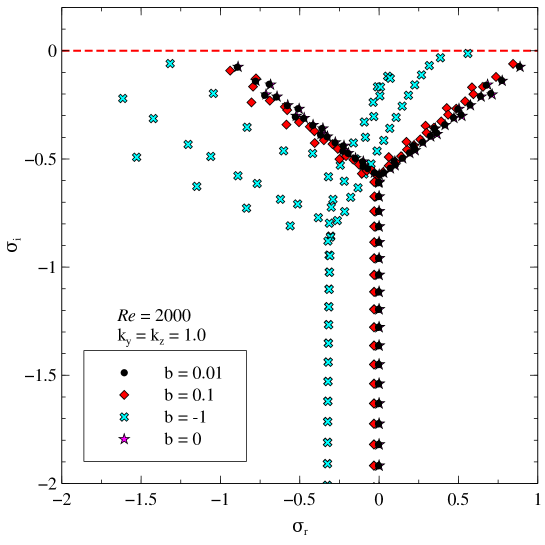
Figure 20: Eigenspectra for background flow $ax+bx^{2}$ for $Re=2000$ and $k_{y}=k_{z}=1$ in the presence of Coriolis force. Here $a=-1$ with different $b$. Note the cases for $b=0$ and $b=0.01$ almost overlap each other.

However, following Farrell & Ioannou (1993), we also can assume that extra force arises only due to perturbation. Hence, the background flow remains intact, the same as linear shear flow. This situation has been explored in Appendix B.

Appendix B Derivation of Orr-Sommerfeld and Squire equations in the presence of Coriolis and external forces

Let us consider small shearing box centered at the radius $r_{0}$ with angular velocity $\Omega_{0}=U_{0}/qL$ with size in $x-$direction 2$L=r-r_{0}$, and we are going to observe the motion of the fluid with respect to that box. The model is described in Mukhopadhyay et al. 2005. The unperturbed velocity for linear shear is

$$\textbf{V}=\left(0,-\frac{U_{0}X}{L},0\right),$$ (55)

where $X$ is dimensionful $x$-coordinate. Again the angular velocity vector $\bm{\omega}=(0,0,\Omega_{0})$ when $\Omega=\Omega_{0}\left(r_{0}/r\right)^{q}$. Now to study the dynamics of a viscous and incompressible rotating fluid, let us consider Navier-Stokes equation in the presence of Coriolis and centrifugal forces, i.e.

$$\begin{split}\frac{\partial\textbf{V}}{\partial t^{\prime}}+(\textbf{V}\cdot\bm{\nabla}^{\prime})\textbf{V}=-\frac{1}{\rho}\bm{\nabla}^{\prime}P-\bm{\omega}\times\bm{\omega}\times\textbf{D}-2\bm{\omega}\times\textbf{V}+\nu\nabla^{\prime 2}\textbf{V}\end{split}$$ (56)

and continuity equation, i.e.

$$\bm{\nabla}^{\prime}\cdot\textbf{V}=0,$$ (57)

where $P$ and $\rho$ are the pressure and density of the fluid respectively.

Here $\textbf{D}=(X,Y,Z)$, $\bm{\nabla}^{\prime}=\left(\frac{\partial}{\partial X},\frac{\partial}{\partial Y},\frac{\partial}{\partial Z}\right)$. To express the above equations in dimensionless variables, we define

$$X=xL,\ Y=yL,\ Z=zL,\ \textbf{V}=U_{0}\textbf{U},\ t^{\prime}=\frac{tL}{U_{0}},\ \textbf{U}=(0,-x,0).$$

Now equation (56) becomes

$$\begin{split}\frac{\partial\textbf{U}}{\partial t}+(\textbf{U}\cdot\bm{\nabla})\textbf{U}+\frac{1}{q^{2}}(\hat{k}\times\hat{k}\times\textbf{d})+\frac{2\hat{k}\times\textbf{U}}{q}+\bm{\nabla}\bar{p}=\frac{1}{Re}\nabla^{2}\textbf{U}\end{split}$$ (58)

and equation (57) becomes

$$\bm{\nabla}\cdot\textbf{U}=0.$$ (59)

Here $\bar{p}=\frac{P}{U_{0}^{2}\rho},\ \textbf{d}=(x,y,z),\ \bm{\nabla}=\left(\frac{\partial}{\partial x},\frac{\partial}{\partial y},\frac{\partial}{\partial z}\right)$ and $Re=\frac{U_{0}L}{\nu}$.

Now we perturb the system and as a result $\textbf{U}(x)\rightarrow\textbf{U}(x)+\textbf{u}^{\prime}(x,y,z,t)$ and $\bar{p}\rightarrow\bar{p}+p^{\prime}(x,y,z,t)$, where $\textbf{u}^{\prime}=(u,v,w)$. Due to the perturbation an extra stochastic force, $\bm{F}(x,y,z,t)$, will arise in the system, as argued by Farrell & Ioannou (1993). Also following Appendix A, we can neglect any effect of force before perturbation.

Hence the evolution equation of perturbation from perturbed Navier-Stokes equation is given by

$$\begin{split}\frac{\partial\textbf{u}^{\prime}}{\partial t}+(\textbf{U}\cdot\bm{\nabla})\textbf{u}^{\prime}+(\textbf{u}^{\prime}\cdot\bm{\nabla})\textbf{U}+\frac{2\hat{k}\times\textbf{u}^{\prime}}{q}+\bm{\nabla}p^{\prime}=\frac{1}{Re}\nabla^{2}\textbf{u}^{\prime}\ -(\textbf{u}^{\prime}\cdot\bm{\nabla})\textbf{u}^{\prime}+\bm{F}(x,y,z,t)\end{split}$$ (60)

and continuity equation becomes

$$\bm{\nabla}\cdot\textbf{u}^{\prime}=0,$$ (61)

when $\bm{F}$ is the final stochastic force. For our convenience we use the following notation:

$$\textbf{U}=(0,U_{y},0);\ U_{y}=U(x)=-x.$$

Componentwise equations (60) and (61) become

$$\left(\frac{\partial}{\partial t}+U_{y}\frac{\partial}{\partial y}\right)u-\frac{2v}{q}+\frac{\partial p^{\prime}}{\partial x}= \frac{1}{Re}\nabla^{2}u\ -(\textbf{u}^{\prime}\cdot\bm{\nabla})u+F_{x}$$ (62)

$$\left(\frac{\partial}{\partial t}+U_{y}\frac{\partial}{\partial y}\right)v+u\frac{\partial U_{y}}{\partial x}+\frac{2u}{q}+\frac{\partial p^{\prime}}{\partial y}= \frac{1}{Re}\nabla^{2}v\ -(\textbf{u}^{\prime}\cdot\bm{\nabla})v+F_{y}$$ (63)

$$\left(\frac{\partial}{\partial t}+U_{y}\frac{\partial}{\partial y}\right)w+\frac{\partial p^{\prime}}{\partial z}= \frac{1}{Re}\nabla^{2}w\ -(\textbf{u}^{\prime}\cdot\bm{\nabla})w+F_{z}$$ (64)

$$\frac{\partial u}{\partial x}+\frac{\partial v}{\partial y}+\frac{\partial w}{\partial z}=0,$$ (65)

where the $x$-component of vorticity is $\zeta=\left(\frac{\partial w}{\partial y}-\frac{\partial v}{\partial z}\right)$.

We further take divergence on both the sides of equation (60) and exploit equation (61) to have

$$\bm{\nabla}\cdot\left\{(\textbf{U}\cdot\bm{\nabla})\textbf{u}^{\prime}\right\}+\bm{\nabla}\cdot\left\{(\textbf{u}^{\prime}\cdot\bm{\nabla})\textbf{U}\right\}+\bm{\nabla}\cdot\frac{2\hat{k}\times\textbf{u}^{\prime}}{q}+\nabla^{2}p^{\prime}=-\bm{\nabla}\cdot[(\textbf{u}^{\prime}\cdot\bm{\nabla})\textbf{u}^{\prime}]+\bm{\nabla}\cdot\bm{F},$$ (66)

where

$$\bm{\nabla}\cdot\left\{(\textbf{U}\cdot\bm{\nabla})\textbf{u}^{\prime}\right\} = \bm{\nabla}\cdot\left(U_{y}\frac{\partial\textbf{u}^{\prime}}{\partial y}\right)$$

$$= \bm{\nabla}U_{y}\cdot\frac{\partial\textbf{u}^{\prime}}{\partial y}+U_{y}\frac{\partial}{\partial y}(\bm{\nabla}\cdot\textbf{u}^{\prime})$$

$$= \frac{\partial U(x)}{\partial x}\frac{\partial u}{\partial y},$$

$$\bm{\nabla}\cdot\left\{(\textbf{u}^{\prime}\cdot\bm{\nabla})\textbf{U}\right\}=\frac{\partial u}{\partial y}\frac{\partial U(x)}{\partial x},$$

$$\bm{\nabla}\cdot\left\{\hat{k}\times\textbf{u}^{\prime}\right\}=-\frac{\partial v}{\partial x}+\frac{\partial u}{\partial y}.$$

Hence,

$$\nabla^{2}p^{\prime}=-\bm{\nabla}\cdot[(\textbf{u}^{\prime}\cdot\bm{\nabla})\textbf{u}^{\prime}]-2\frac{\partial U(x)}{\partial x}\frac{\partial u}{\partial y}+\frac{2}{q}\left(\frac{\partial v}{\partial x}-\frac{\partial u}{\partial y}\right)+\bm{\nabla}\cdot\bm{F}.$$ (67)

If we take gradient and then divergence in equation (62) and also use equation (67), we obtain

$$\begin{split}\left(\frac{\partial}{\partial t}+U\frac{\partial}{\partial y}\right)\nabla^{2}u-\frac{\partial^{2}U}{\partial x^{2}}\frac{\partial u}{\partial y}+\frac{2}{q}\frac{\partial\zeta}{\partial z}=\frac{1}{Re}\nabla^{4}u\ +NL^{u}+F_{1},\end{split}$$ (68)

and if we do partial derivatives with respect to $y$ of equation (64) and with respect to $z$ of the equation (63), and subtract one from the other, we end up with

$$\left(\frac{\partial}{\partial t}+U\frac{\partial}{\partial y}\right)\zeta-\left(\frac{\partial U}{\partial x}+\frac{2}{q}\right)\frac{\partial u}{\partial z}=\frac{1}{Re}\nabla^{2}\zeta+NL^{\zeta}+F_{2},$$ (69)

where $F_{1}$, $F_{2}$, $NL^{u}$ and $NL^{\zeta}$ are given by

$$F_{1}=\left(\nabla^{2}F_{x}-\bm{\nabla}\cdot\frac{\partial\bm{F}}{\partial x}\right),$$ (70)

$$F_{2}=\left(\frac{\partial F_{z}}{\partial y}-\frac{\partial F_{y}}{\partial z}\right),$$ (71)

$$NL^{u}=-\nabla^{2}\cdot[(\textbf{u}^{\prime}\cdot\bm{\nabla})u]+\bm{\nabla}\cdot\frac{\partial}{\partial x}[(\textbf{u}^{\prime}\cdot\bm{\nabla})\textbf{u}^{\prime}],$$ (72)

$$NL^{\zeta}=-\frac{\partial}{\partial y}[(\textbf{u}^{\prime}\cdot\bm{\nabla})w]+\frac{\partial}{\partial z}[(\textbf{u}^{\prime}\cdot\bm{\nabla})v].$$ (73)

If $F_{1}$ and $F_{2}$ happen to be Gaussian in nature, their ensemble average in the present context of biased stochastic system turns out to be non-zero constants, respectively $\Gamma_{1}$ and $\Gamma_{2}$, appeared in equations (1) and (2).

Appendix C Nonlinear terms for threedimensional perturbation

Here we show how to calculate the coefficient of $|A_{t}|^{2}A_{t}$ in equation (31) (i.e. $p$). The nonlinear terms corresponding to equation (24) and (25) are

$$\begin{split}NL^{u}_{1}=i\frac{\partial}{\partial x}\Bigl{[}\bar{u}^{*}_{1}\frac{\partial}{\partial x}(k_{y}\bar{v}_{2}+k_{z}\bar{w}_{2})+2ik_{y}\bar{v}^{*}_{1}(k_{y}\bar{v}_{2}+k_{z}\bar{w}_{2})+2ik_{z}\bar{w}^{*}_{1}(k_{y}\bar{v}_{2}+k_{z}\bar{w}_{2})\Bigr{]}\\ +k^{2}\Bigr{[}\bar{u}^{*}_{1}\frac{\partial\bar{u}_{2}}{\partial x}+2i\bar{u}_{2}(k_{y}\bar{v}^{*}_{1}+k_{z}\bar{w}^{*}_{1})\Bigl{]}\\ +i\frac{\partial}{\partial x}\Bigl{[}\bar{u}_{2}\frac{\partial}{\partial x}(k_{y}\bar{v}^{*}_{1}+k_{z}\bar{w}^{*}_{1})-ik_{y}\bar{v}_{2}(k_{y}\bar{v}^{*}_{1}+k_{z}\bar{w}^{*}_{1})-ik_{z}\bar{w}_{2}(k_{y}\bar{v}^{*}_{1}+k_{z}\bar{w}^{*}_{1})\Bigr{]}\\ +k^{2}\Bigr{[}\bar{u}_{2}\frac{\partial\bar{u}^{*}_{1}}{\partial x}-i\bar{u}^{*}_{1}(k_{y}\bar{v}_{2}+k_{z}\bar{w}_{2})\Bigl{]}\\ =i\frac{\partial}{\partial x}\Bigl{[}\bar{u}^{*}_{1}\frac{\partial}{\partial x}(k_{y}\bar{v}_{2}+k_{z}\bar{w}_{2})+\bar{u}_{2}\frac{\partial}{\partial x}(k_{y}\bar{v}^{*}_{1}+k_{z}\bar{w}^{*}_{1})+i(k_{y}\bar{v}^{*}_{1}+k_{z}\bar{w}^{*}_{1})(k_{y}\bar{v}_{2}+k_{z}\bar{w}_{2})\Bigr{]}\\ +k^{2}\Bigr{[}\frac{\partial}{\partial x}(\bar{u}^{*}_{1}\bar{u}_{2})+2i\bar{u}_{2}(k_{y}\bar{v}^{*}_{1}+k_{z}\bar{w}^{*}_{1})-i\bar{u}^{*}_{1}(k_{y}\bar{v}_{2}+k_{z}\bar{w}_{2})\Bigr{]}\end{split}$$ (74)

and

$$\begin{split}NL^{\zeta}_{1}=-ik_{y}\left(\bar{u}_{2}\frac{\partial\bar{w}^{*}_{1}}{\partial x}+\bar{u}^{*}_{1}\frac{\partial\bar{w}_{2}}{\partial x}\right)+k_{y}^{2}(2\bar{v}^{*}_{1}\bar{w}_{2}-\bar{v}_{2}\bar{w}^{*}_{1})+k_{y}k_{z}\bar{w}^{*}_{1}\bar{w}_{2}\\ +ik_{z}\left(\bar{u}_{2}\frac{\partial\bar{v}^{*}_{1}}{\partial x}+\bar{u}^{*}_{1}\frac{\partial\bar{v}_{2}}{\partial x}\right)-k_{z}^{2}(2\bar{w}^{*}_{1}\bar{v}_{2}-\bar{w}_{2}\bar{v}^{*}_{1})-k_{y}k_{z}\bar{v}^{*}_{1}\bar{v}_{2}.\end{split}$$ (75)

From equations (26), (29) and (19) we have

$$\bar{u}_{1}(x,t)=A_{t}\phi^{u},\ \ \bar{\zeta}_{1}(x,t)=A_{t}\phi^{\zeta},$$ (76)

where we have neglected $\frac{\partial}{\partial x}\Bigl{(}\frac{1}{\mathcal{D}_{t}+i\mathcal{L}}\Bigr{)}\Gamma$ over $\frac{\partial}{\partial t}\Bigl{(}\frac{1}{\mathcal{D}_{t}+i\mathcal{L}}\Bigr{)}\Gamma$, where the former is expected to be much smaller than the latter numerically. In otherwords, we compute nonlinear effects based on the homogeneous part of ($\bar{u}_{1}$, $\bar{v}_{1}$, $\bar{w}_{1}$) and ($\bar{u}_{2}$, $\bar{v}_{2}$, $\bar{w}_{2}$), and their complex conjugates, to the first approximation in equations (24) and (25).

In general, once $u$ and $\zeta$ are known from equations (1) and (2) (irrespective of inclusion of noise/force and nonlinear terms), the other two components of the perturbed velocity field can be obtained from equations

$$-\frac{\partial u}{\partial x} = \frac{\partial v}{\partial y}+\frac{\partial w}{\partial z},$$ (77)

$$\zeta = -\frac{\partial v}{\partial z}+\frac{\partial w}{\partial y}$$ (78)

and the governing equations are

$$\Bigl{(}\frac{\partial^{2}}{\partial z^{2}}+\frac{\partial^{2}}{\partial y^{2}}\Bigr{)}w=-\frac{\partial^{2}u}{\partial z\partial x}+\frac{\partial\zeta}{\partial y},$$ (79)

$$\Bigl{(}\frac{\partial^{2}}{\partial z^{2}}+\frac{\partial^{2}}{\partial y^{2}}\Bigr{)}v=-\frac{\partial^{2}u}{\partial y\partial x}-\frac{\partial\zeta}{\partial z}.$$ (80)

Note, $\bar{v}_{1}$ and $\bar{w}_{1}$ have the same time dependence as $\bar{u}_{1}$ or $\bar{\zeta}_{1}$ has, as the above two equations do not contain time derivative explicitly. They, therefore, can be written as

$$\bar{v}_{1}=A_{t}\phi^{v},\ \ \bar{w}_{1}=A_{t}\phi^{w},$$ (81)

where

$$\phi^{v} = \frac{ik_{y}}{k^{2}}\frac{d\phi^{u}}{dx}+\frac{ik_{z}}{k^{2}}\phi^{\zeta}$$ (82)

and

$$\phi^{w} = \frac{ik_{z}}{k^{2}}\frac{d\phi^{u}}{dx}-\frac{ik_{y}}{k^{2}}\phi^{\zeta},$$ (83)

on substituting $u,\zeta=A_{t}\phi^{u,\zeta}e^{i\textbf{k}\cdot\textbf{r}}$ with $\textbf{k}=(0,k_{y},k_{z})$ and $\textbf{r}=(0,y,z)$ in equations (79) and (80).

The calculations for $u_{2}$, $v_{2}$ and $w_{2}$ are shown in Rajesh 2011.

Appendix D Determination of $\Gamma^{\prime}$

From equation (LABEL:eq:exp_for_Gamma') we have

$$\begin{split}\Gamma^{\prime}=&-\Gamma+i\sigma_{r}\Bigl{(}\frac{1}{\mathcal{D}_{t}+i\mathcal{L}}\Bigr{)}\Gamma.\end{split}$$ (84)

The second term is

$$\frac{1}{\mathcal{D}_{t}+i\mathcal{L}}\Gamma=\frac{\mathcal{D}_{t}-i\mathcal{L}}{\mathcal{D}_{t}^{2}+\mathcal{L}^{2}}\Gamma=\frac{\mathcal{D}_{t}}{\mathcal{D}_{t}^{2}+\mathcal{L}^{2}}\Gamma-\frac{i\mathcal{L}}{\mathcal{D}_{t}^{2}+\mathcal{L}^{2}}\Gamma.$$ (85)

Now, we have

$$\frac{\mathcal{D}_{t}}{\mathcal{D}_{t}^{2}+\mathcal{L}^{2}}\Gamma=\mathcal{D}_{t}^{-2}\mathcal{D}_{t}\Bigl{(}1+\frac{\mathcal{L}^{2}}{\mathcal{D}_{t}^{2}}\Bigr{)}^{-1}\Gamma.$$ (86)

If $||\mathcal{D}_{t}^{2}||>||\mathcal{L}^{2}||$, then the R.H.S. of equation (86) can be written as

$$\begin{split}\mathcal{D}_{t}^{-1}\Bigl{(}1-\frac{\mathcal{L}^{2}}{\mathcal{D}_{t}^{2}}+\frac{\mathcal{L}^{4}}{\mathcal{D}_{t}^{4}}-...\Bigr{)}\Gamma\\ =\Bigl{(}\frac{1}{\mathcal{D}_{t}}-\frac{\mathcal{L}^{2}}{\mathcal{D}_{t}^{3}}+\frac{\mathcal{L}^{4}}{\mathcal{D}_{t}^{5}}-...\Bigr{)}\Gamma\\ =\Bigl{(}t-\mathcal{L}^{2}t^{3}+\mathcal{L}^{4}t^{5}-...\Bigr{)}\Gamma\\ =t\Bigl{(}1-\mathcal{L}^{2}t^{2}+\mathcal{L}^{4}t^{4}-...\Bigr{)}\Gamma\\ =t\Bigl{(}1+\mathcal{L}^{2}t^{2}\Bigr{)}^{-1}\Gamma.\end{split}$$ (87)

Similarly, we have the other term

$$\begin{split}\frac{i\mathcal{L}}{\mathcal{D}_{t}^{2}+\mathcal{L}^{2}}\Gamma=\frac{i\mathcal{L}}{\mathcal{D}_{t}^{2}}\Bigl{(}1+\frac{\mathcal{L}^{2}}{\mathcal{D}_{t}^{2}}\Bigr{)}^{-1}\Gamma\\ =\frac{i\mathcal{L}}{\mathcal{D}_{t}^{2}}\Bigl{(}1-\frac{\mathcal{L}^{2}}{\mathcal{D}_{t}^{2}}+\frac{\mathcal{L}^{4}}{\mathcal{D}_{t}^{4}}-...\Bigr{)}\Gamma\\ =i\mathcal{L}t^{2}(1-\mathcal{L}^{2}t^{2}+\mathcal{L}^{4}t^{4}-...)\Gamma\\ =i\mathcal{L}t^{2}(1+\mathcal{L}^{2}t^{2})^{-1}\Gamma.\end{split}$$ (88)

Hence

$$\Gamma^{\prime}=-\Gamma+i\sigma_{r}(t-i\mathcal{L}t^{2})(1+\mathcal{L}^{2}t^{2})^{-1}\Gamma.$$ (89)

When $t$ is large, the above expression becomes

$$\Gamma^{\prime}=-\Gamma+i\sigma_{r}\Bigl{(}\frac{-i}{\mathcal{L}}\Bigr{)}\Gamma=-\Gamma+\sigma_{r}\Bigl{(}\frac{1}{\mathcal{L}}\Bigr{)}\Gamma.$$ (90)

References

- Afshordi et al. (2005) Afshordi N., Mukhopadhyay B., Narayan R., 2005, ApJ, 629, 373
- Ait-Haddou & Herzog (2003) Ait-Haddou R., Herzog W., 2003, Cell Biochemistry and Biophysics, 38, 191
- Avila (2012) Avila M., 2012, Physical Review Letters, 108, 124501
- Bai (2013) Bai X.-N., 2013, ApJ, 772, 96
- Bai (2017) Bai X.-N., 2017, ApJ, 845, 75
- Bai & Stone (2013) Bai X.-N., Stone J. M., 2013, ApJ, 769, 76
- Balbus & Hawley (1991) Balbus S. A., Hawley J. F., 1991, ApJ, 376, 214
- Balbus et al. (1996) Balbus S. A., Hawley J. F., Stone J. M., 1996, ApJ, 467, 76
- Barker & Latter (2015) Barker A. J., Latter H. N., 2015, MNRAS, 450, 21
- Butler & Farrell (1992) Butler K. M., Farrell B. F., 1992, Physics of Fluids A, 4, 1637
- Cantwell et al. (2010) Cantwell C. D., Barkley D., Blackburn H. M., 2010, Physics of Fluids, 22, 034101
- Carrillo & Goudon (2006) Carrillo J. A., Goudon T., 2006, Communications in Partial Differential Equations, 31, 1349
- Chagelishvili et al. (2003) Chagelishvili G. D., Zahn J. P., Tevzadze A. G., Lominadze J. G., 2003, A&A, 402, 401
- Chandrasekhar (1960) Chandrasekhar S., 1960, Proceedings of the National Academy of Science, 46, 253
- Cuzzi (2007) Cuzzi J., 2007, Nature, 448, 1003
- Das et al. (2018) Das U., Begelman M. C., Lesur G., 2018, MNRAS, 473, 2791
- Dauchot & Daviaud (1995) Dauchot O., Daviaud F., 1995, Physics of Fluids, 7, 335
- Drazin & Reid (2004) Drazin P. G., Reid W. H., 2004, Hydrodynamic Stability
- Dubrulle et al. (2005a) Dubrulle B., Dauchot O., Daviaud F., Longaretti P. Y., Richard D., Zahn J. P., 2005a, Physics of Fluids, 17, 095103
- Dubrulle et al. (2005b) Dubrulle B., Marié L., Normand C., Richard D., Hersant F., Zahn J. P., 2005b, A&A, 429, 1
- Duguet et al. (2010) Duguet Y., Schlatter P., Henningson D. S., 2010, Journal of Fluid Mechanics, 650, 119
- Ellingsen et al. (1970) Ellingsen T., Gjevik B., Palm E., 1970, Journal of Fluid Mechanics, 40, 97
- Farrell & Ioannou (1993) Farrell B. F., Ioannou P. J., 1993, Physics of Fluids A, 5, 2600
- Fromang & Papaloizou (2007) Fromang S., Papaloizou J., 2007, A&A, 476, 1113
- Gammie & Menou (1998) Gammie C. F., Menou K., 1998, ApJ, 492, L75
- Gogichaishvili et al. (2017) Gogichaishvili D., Mamatsashvili G., Horton W., Chagelishvili G., Bodo G., 2017, ApJ, 845, 70
- Hawley et al. (1999) Hawley J. F., Balbus S. A., Winters W. F., 1999, ApJ, 518, 394
- Henning & Stognienko (1996) Henning T., Stognienko R., 1996, A&A, 311, 291
- Ioannou & Kakouris (2001) Ioannou P. J., Kakouris A., 2001, ApJ, 550, 931
- Kim & Ostriker (2000) Kim W.-T., Ostriker E. C., 2000, ApJ, 540, 372
- Klahr & Bodenheimer (2003) Klahr H. H., Bodenheimer P., 2003, ApJ, 582, 869
- Klahr & Hubbard (2014) Klahr H., Hubbard A., 2014, ApJ, 788, 21
- Latter (2016) Latter H. N., 2016, MNRAS, 455, 2608
- Lesur & Longaretti (2005) Lesur G., Longaretti P.-Y., 2005, A&A, 444, 25
- Lin (1961) Lin C. C., 1961, Journal of Fluid Mechanics, 10, 430
- Lin & Youdin (2015) Lin M.-K., Youdin A. N., 2015, ApJ, 811, 17
- Lithwick (2007) Lithwick Y., 2007, ApJ, 670, 789
- Lithwick (2009) Lithwick Y., 2009, ApJ, 693, 85
- Lominadze et al. (1988) Lominadze D. G., Chagelishvili G. D., Chanishvili R. G., 1988, Soviet Astronomy Letters, 14, 364
- Lynden-Bell & Pringle (1974) Lynden-Bell D., Pringle J. E., 1974, MNRAS, 168, 603
- Mahajan & Krishan (2008) Mahajan S. M., Krishan V., 2008, ApJ, 682, 602
- Mamatsashvili et al. (2013) Mamatsashvili G. R., Chagelishvili G. D., Bodo G., Rossi P., 2013, MNRAS, 435, 2552
- Mamatsashvili et al. (2016) Mamatsashvili G., Khujadze G., Chagelishvili G., Dong S., Jiménez J., Foysi H., 2016, Phys. Rev. E, 94, 023111
- Marcus et al. (2013) Marcus P. S., Pei S., Jiang C.-H., Hassanzadeh P., 2013, Physical Review Letters, 111, 084501
- Marcus et al. (2015) Marcus P. S., Pei S., Jiang C.-H., Barranco J. A., Hassanzadeh P., Lecoanet D., 2015, ApJ, 808, 87
- Menou (2000) Menou K., 2000, Science, 288, 2022
- Menou & Quataert (2001) Menou K., Quataert E., 2001, ApJ, 552, 204
- Mukhopadhyay (2013) Mukhopadhyay B., 2013, Physics Letters B, 721, 151
- Mukhopadhyay & Chattopadhyay (2013) Mukhopadhyay B., Chattopadhyay A. K., 2013, Journal of Physics A Mathematical General, 46, 035501
- Mukhopadhyay et al. (2005) Mukhopadhyay B., Afshordi N., Narayan R., 2005, ApJ, 629, 383
- Mukhopadhyay et al. (2011a) Mukhopadhyay B., Mathew R., Raha S., 2011a, New Journal of Physics, 13, 023029
- Mukhopadhyay et al. (2011b) Mukhopadhyay B., Mathew R., Raha S., 2011b, New Journal of Physics, 13, 023029
- Mukhopadhyay et al. (2011c) Mukhopadhyay B., Mathew R., Raha S., 2011c, New Journal of Physics, 13, 023029
- Nath & Mukhopadhyay (2015) Nath S. K., Mukhopadhyay B., 2015, Phys. Rev. E, 92, 023005
- Nath & Mukhopadhyay (2016) Nath S. K., Mukhopadhyay B., 2016, ApJ, 830, 86
- Nelson et al. (2013) Nelson R. P., Gressel O., Umurhan O. M., 2013, MNRAS, 435, 2610
- Ormel et al. (2008) Ormel C. W., Cuzzi J. N., Tielens A. G. G. M., 2008, ApJ, 679, 1588
- Paoletti et al. (2012) Paoletti M. S., van Gils D. P. M., Dubrulle B., Sun C., Lohse D., Lathrop D. P., 2012, A&A, 547, A64
- Parrondo & Español (1996) Parrondo J. M. R., Español P., 1996, American Journal of Physics, 64, 1125
- Peskin (2002) Peskin C. S., 2002, Acta Numerica, 11, 479–517
- Pessah & Psaltis (2005) Pessah M. E., Psaltis D., 2005, ApJ, 628, 879
- Pumir (1996) Pumir A., 1996, Physics of Fluids, 8, 3112
- Rajesh (2011) Rajesh S. R., 2011, MNRAS, 414, 691
- Razdoburdin (2020) Razdoburdin D. N., 2020, Monthly Notices of the Royal Astronomical Society, 492, 5366
- Richard & Zahn (1999) Richard D., Zahn J.-P., 1999, A&A, 347, 734
- Rincon et al. (2007) Rincon F., Ogilvie G. I., Cossu C., 2007, A&A, 463, 817
- Rüdiger & Zhang (2001) Rüdiger G., Zhang Y., 2001, A&A, 378, 302
- Salmeron & Wardle (2004) Salmeron R., Wardle M., 2004, Ap&SS, 292, 451
- Salmeron & Wardle (2005) Salmeron R., Wardle M., 2005, MNRAS, 361, 45
- Salmeron & Wardle (2008) Salmeron R., Wardle M., 2008, MNRAS, 388, 1223
- Schmid & Henningson (2001) Schmid P., Henningson D., 2001, Stability and Transition in Shear Flows. Applied Mathematical Sciences, Springer New York, https://books.google.co.in/books?id=5eNoy2VdXo8C
- Schmid et al. (2002) Schmid P., Henningson D., Jankowski D., 2002, Applied Mechanics Reviews, 55, B57
- Sekimoto et al. (2016) Sekimoto A., Dong S., Jiménez J., 2016, Physics of Fluids, 28, 035101
- Shakura & Sunyaev (1973) Shakura N. I., Sunyaev R. A., 1973, A&A, 24, 337
- Shen et al. (2006) Shen Y., Stone J. M., Gardiner T. A., 2006, ApJ, 653, 513
- Shi et al. (2017) Shi L., Hof B., Rampp M., Avila M., 2017, Physics of Fluids, 29, 044107
- Singh Bhatia & Mukhopadhyay (2016) Singh Bhatia T., Mukhopadhyay B., 2016, Physical Review Fluids, 1, 063101
- Stoll & Kley (2014) Stoll M. H. R., Kley W., 2014, A&A, 572, A77
- Stoll & Kley (2016) Stoll M. H. R., Kley W., 2016, A&A, 594, A57
- Tevzadze et al. (2003) Tevzadze A. G., Chagelishvili G. D., Zahn J. P., Chanishvili R. G., Lominadze J. G., 2003, A&A, 407, 779
- Umurhan et al. (2016) Umurhan O. M., Nelson R. P., Gressel O., 2016, A&A, 586, A33
- Velikhov (1959) Velikhov E., 1959, Zhur. Eksptl’. i Teoret. Fiz., Vol: 36
- Yecko (2004a) Yecko P. A., 2004a, A&A, 425, 385
- Yecko (2004b) Yecko P. A., 2004b, A&A, 425, 385
- van Oudenaarden & Boxer (1999) van Oudenaarden A., Boxer S. G., 1999, Science, 285, 1046