Rank $N$ Vafa-Witten invariants, modularity and blow-up

Abstract:

We derive explicit expressions for the generating functions of refined Vafa-Witten invariants $\Omega(\gamma,y)$ of $\mathds{P}^{2}$ of arbitrary rank $N$ and for their non-holomorphic modular completions. In the course of derivation we also provide: i) a generalization of the recently found generating functions of $\Omega(\gamma,y)$ and their completions for Hirzebruch and del Pezzo surfaces in the canonical chamber of the moduli space to a generic chamber; ii) a version of the blow-up formula expressed directly in terms of these generating functions and its reformulation in a manifestly modular form.

1 Introduction

The topologically twisted $\mathcal{N}=4$ super Yang-Mills [1] on a complex surface $S$, also known as Vafa-Witten (VW) theory, appears to be at the heart of intersection of various theories, problems, approaches and conjectures in mathematics and physics. On one hand, its partition function captures important topological information about the surface $S$ encoded in the so called Vafa-Witten invariants, the Euler numbers of the moduli spaces of semi-stable sheaves on $S$, which are the same as the moduli spaces of instantons in the topologically twisted gauge theory. The evaluation of these invariants is an important problem that has many links to other mathematical subjects. In particular, it turns out that the generating functions of VW invariants exhibit non-trivial modular properties and provide examples of either modular or mock modular forms [2, 3]. This fact makes them a beautiful playground for number theory that can be used as a source for new ideas and identities.

On the other hand, the same invariants can be interpreted as BPS indices in supersymmetric gauge theory, while their modular properties are understood as a consequence of S-duality [4, 1]. Moreover, they can be related to generalized Donaldson-Thomas (DT) invariants of non-compact Calabi-Yau (CY) threefolds because VW theory appears as an effective theory of M5-branes wrapped on $S\times T^{2}$ and reduced along the torus where $S$ is a divisor of a CY. Regarding these non-compact manifolds as local limits of compact CYs establishes further relations with physics of BPS black holes, instantons and topological strings (see e.g. [5]).

The connection to string theory outlined above furnishes us with a plethora of methods based on dualities and other physical considerations that can bring new insights into the problem of evaluation of VW invariants and understanding their modular properties. In particular, recently an important progress has been achieved due to a complete characterization of a modular anomaly of the generating functions of certain BPS indices in string theory compactifications with $N=2$ supersymmetry [6, 7]. More precisely, reducing from M-theory to type IIA string, the above M5-brane system gives rise to a bound state of D4-D2-D0-branes wrapped on even dimensional cycles of a compact Calabi-Yau threefold $\mathfrak{Y}$, which at strong coupling corresponds to a BPS black hole with a set of electro-magnetic charges. Hence, it makes sense to consider a generating function of black hole degeneracies (obtained by summing over D0-brane charge), whose mathematical interpretation is the generating function of the generalized DT invariants counting semi-stable coherent sheaves supported on a divisor $\mathcal{D}\subset\mathfrak{Y}$. Whereas for $\mathcal{D}$ irreducible the generating function, evaluated in the so-called attractor chamber of the moduli space, is known to be a modular form under S-duality group $SL(2,\mathds{Z})$ [8, 9, 10], for reducible divisors where $\mathcal{D}=\sum_{i=1}^{n}\mathcal{D}_{i}$ it exhibits a modular anomaly [11]. Remarkably, the anomaly turns out to be of a very special type and can be completely characterized by constructing modular completions of the generating functions, i.e. their non-holomorphic deformations which do transform as modular forms. Using duality constraints of string theory, in [6] a general formula for such completion in terms of the original holomorphic generating functions has been found for a generic divisor. Its form implies that the generating functions are actually vector valued higher depth mock modular forms, objects generalizing the notion of the usual mock modularity [18].

Then in [7] this construction has been upgraded to include a refinement parameter $y$. Its logarithm $z=\frac{\log y}{2\pi\mathrm{i}}$ transforms as an elliptic parameter so that the refined generating functions turn out to be higher depth mock Jacobi forms. Amazingly, the refined construction is in fact much simpler than the unrefined one and thus represents a natural framework for further developments. In particular, taking the local limit on $\mathfrak{Y}$ given by the canonical bundle over a complex surface $S$ with $b_{2}^{+}(S)=1$ and $b_{1}(S)=0$, it has been used to get a formula for the modular completion $\widehat{h}_{N,\mu}(\tau,z)$ of the generating functions $h_{N,\mu}(\tau,z)$ of refined VW invariants of $S$ with $U(N)$ gauge group [7]. The point is that for this class of surfaces such generating functions are known to have a modular anomaly [1], which can be traced back to the existence of non-holomorphic contributions to the partition function of VW theory generated by Q-exact terms and coming from boundaries of the moduli space [19]. They ensure that the partition function is a true modular form given by the non-holomorphic completion of the holomorphic generating functions.

Note that the formula of [7] only expresses $\widehat{h}_{N,\mu}$ in terms of $h_{N_{i},\mu_{i}}$ with $N_{i}\leq N$, which remained unknown at that stage. Nevertheless, it allows to trade the modular anomaly of the generating functions for the holomorphic anomaly of their completions. Combined with the requirement to have a well-defined unrefined limit $z\to 0$, it can then be used to actually find the generating functions themselves, similarly to solution of the topological string on elliptic CY threefolds [20, 21]. This program has been realized for Hirzebruch and del Pezzo surfaces, ${\mathbb{F}}_{m}$ and ${\mathbb{B}}_{m}$, in [22] which produced a closed formula for both $h_{N,\mu}$ and $\widehat{h}_{N,\mu}$ for all ranks $N$. (For earlier results on VW invariants of these surfaces, see [23, 24, 25, 26, 27, 28].)

This result however has two omissions. First, as indicated above, the generating functions $h_{N,\mu}$ count the invariants only in a special chamber of the moduli space, parametrized by a choice of polarization of $S$ provided by the Kähler form $J\in H^{2}(S,\mathds{R})$. This chamber corresponds to the attractor chamber of the CY geometry and, in the terminology of [28], is called the canonical chamber, specified by $J=-K_{S}=c_{1}(S)$ where $K_{S}$ is the canonical class and $c_{1}(S)$ is the first Chern class of the surface. In other chambers the invariants may have different values due to the wall-crossing phenomenon. Although there are well established wall-crossing formulae which allow to compute the change of invariants from one chamber to another [29, 30, 31], it is certainly desirable to have an explicit formula for the generating functions in arbitrary chamber.

Second, the construction of [22] relied on the existence of a null vector belonging to the integer homology lattice $\Lambda_{S}=H_{2}(S,\mathds{Z})$. Clearly, such vector does not exist in the case $b_{2}(S)=1$ corresponding to $S=\mathds{P}^{2}$. Thus, this case remained uncaptured by the that construction.

In fact, the VW invariants of $\mathds{P}^{2}$ are determined by those of ${\mathbb{F}}_{1}$ by means of the blow-up formula [32, 33, 34]. However this formula does not apply directly to $h_{N,\mu}$. Instead, one has to go to a different chamber of the moduli space and pass through the so-called stack invariants [35]. In principle, this is not a big deal and this procedure has been realized for any $N$ in [36], generalizing previous results in [37, 38, 26] and expressing the generating functions as combinations of generalized Appell functions. However, the corresponding result for the completion, which is important not only as a characterization of the modular properties of the VW invariants, but also as a prediction for the partition function of the physical theory, was missing so far. Of course, it can be obtained by either substituting the generating functions of [36] into the formula for the completion of [7], or by applying the general procedure developed in [39] for constructing modular completions of indefinite theta series and generalized Appell functions. But the former approach leads to expressions with obscure modular properties, whereas the latter is very cumbersome and has been realized so far only for $N=3$ [40]. On the other hand, the construction of [22] is designed to produce manifestly modular expressions for completions, so that it is natural to try whether it can encompass the case of $\mathds{P}^{2}$ as well. Besides, this might be useful keeping in mind its possible extension to finding DT invariants of compact CY threefolds where the existence of a null vector belonging to the lattice is not guarantied either.

In this paper we fill in the above two gaps. First, we conjecture (see eq. (2.19)) an explicit expression for the generating functions of refined VW invariants of Hirzebruch and del Pezzo surfaces for a two-parameter family of polarizations $J$ (which exhaust all possible $J$ in the case of ${\mathbb{F}}_{m}$). Next, we show how one can avoid the obstruction of the absence of a null vector in $\Lambda_{S}$: to this end, the formula for the modular completion $\widehat{h}_{N,\mu}$ can be rewritten in terms of a set of functions $\check{h}_{N,\check{\mu}}$ defined by an ‘extended lattice’ $\check{\Lambda}_{S}=\Lambda_{S}\oplus\mathds{Z}$ that can already possess such a vector. Then the construction of [22] allows to find both $\check{h}_{N,\check{\mu}}$ and their completions $\hbox to0.0pt{$\displaystyle\widehat{\check{h}}$\hss}\phantom{h}_{N,\check{\mu}}$, while $h_{N,\mu}$ and $\widehat{h}_{N,\mu}$ follow from them in a trivial way.

It turns out that a particular case of this construction is nothing else but a variant of the blow-up formula. However, it differs from the standard formula in that it is written directly in terms of the generating functions of VW invariants and does not require the use of stack invariants. It can also be written in a way which is manifestly modular with respect to the full duality group $SL(2,\mathds{Z})$ (see eq. (3.11)), whereas usually only invariance under its congruence subgroup is apparent. Thus, in a sense, our derivation provides a proof of consistency of the blow-up formula with modularity for any rank $N$.

Specializing the above results for the case of $\mathds{P}^{2}$ allows to obtain explicit expressions for both $h^{\,\mathds{P}^{2}}_{N,\mu}$ and $\widehat{h}^{\,\mathds{P}^{2}}_{N,\mu}$. The formula (4.3) for the modular completion is the main new result of this work.

The organization of the paper is as follows. In the next section we review the results of [22] for $S={\mathbb{F}}_{m}$ and ${\mathbb{B}}_{m}$ obtained in the canonical chamber of the moduli space and extend them to other chambers. In section 3 we present our construction based on the extended lattice, that allows to find generating functions in the absence of a null vector in $\Lambda_{S}$, and relate it to the blow-up formula. Then in section 4 we apply it to the case of $\mathds{P}^{2}$. Section 5 presents our conclusions. Appendices contain useful details on theta functions, stack invariants, the blow-up formula and generalized error functions.

2 Generating functions of refined Vafa-Witten invariants

In this section we define the refined VW invariants, their generating functions and discuss them for Hirzebruch and del Pezzo surfaces. The basic definitions are collected in $\S$2.1. Then in $\S$2.2 we present the formula for $h_{N,\mu}$ in the canonical chamber found in [22]. In $\S$2.3 it is generalized to a two-parameter family of polarizations. Finally, in $\S$2.4 we provide explicit results for the modular completions $\widehat{h}_{N,\mu}$.

2.1 Refined VW invariants

Vafa-Witten invariants of a surface $S$ are defined as Euler numbers of the moduli spaces $\mathcal{M}_{\gamma,J}$ of semi-stable coherent sheaves on $S$ where $\gamma=(N,\mu,{1\over 2}\mu^{2}-n)$ is the Chern character of the sheaf and $J$ is a polarization entering the stability condition. From physics point of view, $N$ is the rank of the gauge group $U(N)$, $J$ is the Kähler form, whereas $\mu=-c_{1}(F)\in\Lambda_{S}$ and $n=\int_{S}c_{2}(F)\in\mathds{Z}$ are Chern classes of the gauge bundle. The moduli space $\mathcal{M}_{\gamma,J}$ parametrizes solutions of hermitian Yang-Mills equations and depends on $J$ through the self-duality condition on the field strength $F$. An important property, corresponding to the spectral flow symmetry, is that the moduli space does not change upon tensoring $F$ with a line bundle $\mathcal{L}$. This leads to the shift $\mu\to\mu-Nc_{1}(\mathcal{L})$, but leaves invariant the rank $N$ and the Bogomolov discriminant

$$\Delta(F):=\frac{1}{N}\left(n-\frac{N-1}{2N}\mu^{2}\right),$$ (2.1)

where $\mu^{2}\equiv\int_{S}\mu^{2}$. Due to this, the parameter $\mu$ can be restricted to $\Lambda_{S}/N\Lambda_{S}$.

In this paper we will be interested in the refined VW invariants, which are defined by Poincaré polynomials of $\mathcal{M}_{\gamma,J}$. More precisely, they are given by

$$\Omega_{J}(\gamma,y)=\frac{\sum_{p=0}^{d}y^{2p-d_{\mathds{C}}(\mathcal{M}_{\gamma,J})}\,b_{p}(\mathcal{M}_{\gamma,J})}{y-y^{-1}}\,,$$ (2.2)

where $y=e^{2\pi\mathrm{i}z}$ is the refinement parameter, $d_{\mathds{C}}(\mathcal{M})$ is the complex dimension of $\mathcal{M}$ and $b_{p}(\mathcal{M})$ is its Betti number. The parameter $z$ is taken to be complex $z=\alpha-\tau\beta$ with both $\alpha$ and $\beta$ non-vanishing. To exhibit modular properties of the refined invariants, one has to work actually in terms of their rational counterparts [41, 40]

$$\bar{\Omega}_{J}(\gamma,y)=\sum_{m|\gamma}\frac{1}{m}\,\Omega_{J}(\gamma/m,-(-y)^{m}).$$ (2.3)

It is these invariants that we use to define the generating functions

$$h^{S}_{N,\mu,J}(\tau,z)=\sum_{n\geq 0}\bar{\Omega}_{J}(\gamma,y)\,\mbox{q}^{N\left(\Delta(F)-\tfrac{\chi(S)}{24}\right)},$$ (2.4)

where as usual $\mbox{q}=e^{2\pi\mathrm{i}\tau}$. As follows from (2.2), this function has single poles at $z=0$ and $z={1\over 2}$ with the residues given by the generating function of the unrefined VW invariants.

For $N=1$, there is no dependence on $\mu$ and $J$, and the generating function is known for any $S$ [42]. For surfaces with $b_{1}(S)=0$, it is given by

$$h^{S}_{1,0}(\tau,z)=\frac{\mathrm{i}}{\theta_{1}(\tau,2z)\,\eta(\tau)^{b_{2}(S)-1}},$$ (2.5)

where $\theta_{1}(\tau,z)$ is the Jacobi theta function and $\eta(\tau)$ is the Dedekind eta function. For higher ranks one obtains already a vector valued function with components labelled by $\mu\in\Lambda_{S}/N\Lambda_{S}$. Regarding dependence on $J$, when $b_{2}^{+}(S)>1$ it was found to be absent, but for $b_{2}^{+}(S)=1$ and $b_{2}(S)>1$ it does affect the generating functions. Of course, this dependence is piecewise constant and can be captured by the standard wall-crossing formulae [29, 30, 31]. In the following, we will be interested in surfaces with $b_{2}^{+}(S)=1$ and $b_{1}(S)=0$ which include, in particular, Hirzebruch ${\mathbb{F}}_{m}$, del Pezzo ${\mathbb{B}}_{m}$ and $\mathds{P}^{2}$. Thus, for all of them except $\mathds{P}^{2}$ there is a non-trivial wall-crossing.

2.2 Generating functions for ${\mathbb{F}}_{m}$ and ${\mathbb{B}}_{m}$: canonical chamber

Among all possible choices of polarization $J$ there is one special $J=-K_{S}$ which corresponds to the canonical chamber in the moduli space. On one hand, this is the chamber with the richest BPS spectrum [28]. On the other hand, after uplifting to a CY threefold, it corresponds to the attractor chamber of the CY moduli space where the moduli are fixed by the charges and one expects that no bound states are present [43] (except the so-called scaling solutions [44, 45]). This is the chamber where the construction of [6, 7] applies, and in [22] it was used to get an explicit formula for the generating functions $h^{S}_{N,\mu}:=h^{S}_{N,\mu,-K_{S}}$ for Hirzebruch and del Pezzo surfaces, which we now review.

First, let us recall a few basic facts about these surfaces. The Hirzebruch surface ${\mathbb{F}}_{m}$ is a projectivization of the $\mathcal{O}(m)\oplus\mathcal{O}(0)$ bundle over $\mathds{P}^{1}$. It has $b_{2}(S)=2$ and in the basis given by the curves corresponding to the fiber $[f]$ and the section of the bundle $[s]$, the intersection matrix and the first Chern class are the following

$$C_{\alpha\beta}=\begin{pmatrix}0&1\\ 1&-m\end{pmatrix},\qquad c_{1}({\mathbb{F}}_{m})=(m+2)[f]+2[s].$$ (2.6)

The del Pezzo surface ${\mathbb{B}}_{m}$ is the blow-up of $\mathds{P}^{2}$ over $m$ generic points. It has $b_{2}(S)=m+1$ and a basis of $\Lambda_{{\mathbb{B}}_{m}}$ is given by the hyperplane class of $\mathds{P}^{2}$ and the exceptional divisors of the blow-up denoted, respectively, by $D_{1}$ and $D_{2},\dots,D_{m+1}$. In this basis the intersection matrix and the first Chern class are given by

$$C_{\alpha\beta}={\rm diag}(1,-1,\dots,-1),\qquad c_{1}({\mathbb{B}}_{m})=3D_{1}-\sum_{\alpha=2}^{m+1}D_{\alpha}.$$ (2.7)

A few comments are in order:

• For all above surfaces as well as for $\mathds{P}^{2}$, the signature of the intersection matrix is $(1,b_{2}-1)$ and

  $$c_{1}^{2}(S)=10-b_{2}(S).$$ (2.8)

• In fact, ${\mathbb{F}}_{1}={\mathbb{B}}_{1}$, i.e. it is the blow-up of $\mathds{P}^{2}$ at one point, and by changing the basis to

  $$D_{1}=[f]+[s],\qquad D_{2}=[s],$$ (2.9)

  one brings $C_{\alpha\beta}$ and $c_{1}({\mathbb{F}}_{1})$ to the form (2.7) with $m=1$.

• The crucial role in the construction of the generating functions of VW invariants is played by a null vector $v_{0}\in\Lambda_{S}$. For $S={\mathbb{F}}_{m}$ and ${\mathbb{B}}_{m}$, this vector must be chosen as follows [22]

  $$v_{0}({\mathbb{F}}_{m})=[f],\qquad v_{0}({\mathbb{B}}_{m})=D_{1}-D_{2}.$$ (2.10)

Next, one has to introduce several notations. Let $\hat{\gamma}=(N,q)$ where $q\in\Lambda_{S}+\frac{N}{2}K_{S}$ and it is further decomposed into the part spanning $N\Lambda_{S}$ and the residue class $\mu\in\Lambda_{S}/N\Lambda_{S}$, that reflects the spectral flow symmetry. In a basis $D_{\alpha}$, $\alpha=1,\dots,b_{2}(S)$, of $H_{2}(S,\mathds{Z})$ this decomposition is given by

$$q_{\alpha}=N\,C_{\alpha\beta}\epsilon^{\beta}+\mu_{\alpha}-\frac{N}{2}\,C_{\alpha\beta}c_{1}^{\beta},\qquad\epsilon^{\alpha}\in\mathds{Z},$$ (2.11)

where $C_{\alpha\beta}=D_{\alpha}\cap D_{\beta}$ and $c_{1}^{\alpha}$ are the components of the first Chern class $c_{1}(S)=-K_{S}=c_{1}^{\alpha}D_{\alpha}$ of the surface. Then we introduce a combination of theta series

$$\Theta^{S}_{N,\mu}(\tau,z;\{\Phi_{n}\})=\sum_{n=1}^{\infty}\frac{1}{2^{n-1}}\sum_{\sum_{i=1}^{n}\hat{\gamma}_{i}=\hat{\gamma}}\Phi_{n}(\{\hat{\gamma}_{i}\})\,\mbox{q}^{{1\over 2}Q_{n}(\{\hat{\gamma}_{i}\})}\,y^{\sum_{i<j}\gamma_{ij}(c_{1}(S))}\prod_{i=1}^{n}H^{S}_{N_{i},\mu_{i}}(\tau,z),$$ (2.12)

where the sum goes over all decompositions of the charge $\hat{\gamma}=(N,\mu-\frac{N}{2}c_{1})$, i.e. with the spectral flow parameter set to zero, and the charges $q_{i}$ are quantized as in (2.11) with $N$ replaced by $N_{i}$. The other notations used in (2.12) are the following:

• the quadratic form $Q_{n}$ given by

  $$Q_{n}(\{\hat{\gamma}_{i}\})=\frac{1}{N}\,q^{2}-\sum_{i=1}^{n}\frac{1}{N_{i}}q_{i}^{2}=-\sum_{i<j}\frac{(N_{i}q_{j}-N_{j}q_{i})^{2}}{NN_{i}N_{j}}\,,$$ (2.13)

  where $q^{2}=C^{\alpha\beta}q_{\alpha}q_{\beta}$ and $C^{\alpha\beta}$ is the inverse of $C_{\alpha\beta}$; for the charges satisfying $\sum_{i}q_{i}=q$ with $q$ fixed, the signature of $Q_{n}$ is $(n-1,(n-1)(b_{2}-1))$;

• anti-symmetrized Dirac product of charges depending on a vector $v\in\Lambda_{S}$

  $$\gamma_{ij}(v)=v^{\alpha}(N_{i}q_{j,\alpha}-N_{j}q_{i,\alpha});$$ (2.14)

• the generating function $H^{S}_{N,\mu}$ of stack invariants evaluated at $J=v_{0}$, which is given in (B.7),

• the kernels $\Phi_{n}$ depending on $n$ charges that determine the theta series and will be specified below.

Note that both (2.13) and (2.14) are invariant under an overall shift of the spectral flow parameters $\epsilon_{i}^{\alpha}$. The same is supposed to be true (and indeed will be) for the kernels $\Phi_{n}$. Therefore, the r.h.s. of (2.12) is invariant under the spectral flow shift of $q$, which explains why this symmetry is fixed in $\hat{\gamma}$.

The main result of [22] is that the generating functions of refined VW invariants in the canonical chamber are expressed through the combinations (2.12)

$$h^{S}_{N,\mu}=\Theta^{S}_{N,\mu}(\tau,z;\{\Phi_{n}(-K_{S})\})$$ (2.15)

with the following kernels

$$\Phi_{n}(\{\hat{\gamma}_{i}\};v)=\sum_{\mathcal{J}\subseteq\mathscr{Z}_{n-1}}\left[e_{|\mathcal{J}|}\,\delta_{\mathcal{J}}(v)\prod_{k\in\mathscr{Z}_{n-1}\setminus\mathcal{J}}\Bigl{(}\mbox{\rm sgn}(\Gamma_{k}(v))-\mbox{\rm sgn}(\mathscr{B}_{k})\Bigr{)}\right],$$ (2.16)

where $\mathscr{Z}_{n}=\{1,\dots,n\}$, $|\mathcal{J}|$ is the cardinality of the set, $e_{m-1}$ is the $m$-th Taylor coefficient of ${\rm arctanh}$, namely

$$e_{m}=\left\{\begin{array}[]{cc}0&\mbox{ if }m\mbox{ is odd},\\ \frac{1}{m+1}&\mbox{ if }m\mbox{ is even},\end{array}\right.$$ (2.17)

$\delta_{\mathcal{J}}(v)=\prod_{k\in\mathcal{J}}\delta_{\Gamma_{k}(v)}$ is the product of Kronecker deltas, and

$$\begin{split}\Gamma_{k}(v)=&\,\sum_{i=1}^{k}\sum_{j=k+1}^{n}\gamma_{ij}(v),\\ \mathscr{B}_{k}=&\,\gamma_{k,k+1}(v_{0})+\beta N_{k}N_{k+1}(N_{k}+N_{k+1})\,v_{0}\cdot c_{1}(S).\end{split}$$ (2.18)

The structure of the kernel (2.16) is in fact very simple. Generically, it is given by a product of differences of two sign functions. This is a typical structure for a kernel of indefinite theta series ensuring their convergence [39]. In our case, one set of sign functions is determined by the null vector $v_{0}$ (2.10) and the second by the vector $v$, which according to (2.15) is equal to the anti-canonical class $-K_{S}=c_{1}(S)$. However, for some values of charges the arguments of the second set may vanish. Such situations require a special attention. The formula (2.16) is written using convention $\mbox{\rm sgn}(0)=0$, however it turns out that the construction taking its roots in modularity requires, roughly speaking, that a product of even number of sign functions with vanishing arguments is to be replaced by the non-vanishing number $e_{m}$, i.e. $(\mbox{\rm sgn}(0))^{m}\to e_{m}$. This is the origin of the sum over subsets in (2.16).

2.3 Generating functions for ${\mathbb{F}}_{m}$ and ${\mathbb{B}}_{m}$: generic chamber

Given the result (2.15), it is easy to guess an expression for the generating functions for a more general polarization $J$:

Conjecture 1.

For $J\in\mbox{\rm Span}(c_{1}(S),v_{0}(S))^{+}$, where $v_{0}(S)$ is specified in (2.10) and $+$ indicates the restriction to the Kähler cone, one has

$$\framebox{$h^{S}_{N,\mu,J}=\Theta^{S}_{N,\mu}(\tau,z;\{\Phi_{n}(J)\})$}$$ (2.19)

Note that for $S={\mathbb{F}}_{m}$ the restriction on $J$ is empty since $\mbox{\rm Span}(c_{1}(S),v_{0})^{+}$ coincides with the full Kähler cone. On the other hand, for $S={\mathbb{B}}_{m}$ it restricts $J$ to belong to a two-dimensional plane in the $m+1$ dimensional moduli space. This restriction is necessary because for more general $J$ the formula (2.19) appears to not have a well-defined unrefined limit and to be inconsistent with the formula for the completion (2.24) given below (see footnote 7).

We will not try to prove this conjecture. Instead, we provide several evidences in its favor:

• We have checked numerically that it agrees with the formulae for $h^{{\mathbb{F}}_{m}}_{N,\mu,J_{k,\ell}}$, $N=2,3$, where $J_{k,\ell}=k([s]+m[f])+\ell[f]$, $k,\ell\geq 0$, which were given in [26], provided one does not hit a wall of marginal stability what may happen for $J\cdot\mu=0\!\!\mod N$.

• In the canonical chamber $J=-K_{S}$ it reduces to the result (2.15).

• For $J=v_{0}$ it reduces to the generating function of stack invariants $H^{S}_{N,\mu}$ (B.7) plus the so-called ‘zero mode contributions’ where some of the charges are fixed by the condition that at least one of $\Gamma_{k}(v_{0})$ vanishes. This is the expected structure since the zero mode contributions account for the difference between stack and VW invariants.

• As we will se below, it nicely agrees with the blow up formula.

2.4 Modular completion

As explained in the Introduction, the result (2.15) has been derived by requiring a proper behavior under modular transformations which act on the arguments of the generating functions in the following way

$$\tau\to\frac{a\tau+b}{c\tau+d}\,,\qquad z\to\frac{z}{c\tau+d}\,,\qquad\left(\begin{array}[]{cc}a&b\\ c&d\end{array}\right)\in SL(2,\mathds{Z}).$$ (2.20)

Identifying $\tau$ with the complexified coupling constant of $\mathcal{N}=4$ super-Yang-Mills, one recognizes in (2.20) the standard S-duality which leaves this theory invariant. This suggests that the partition function of VW theory transforms as a modular form. Furthermore, since the dependence on $\bar{\tau}$ can be shown to be Q-exact [1], the standard arguments imply that the partition function is holomorphic in $\tau$ and is essentially captured (up to a simple theta series) by the generating function $h_{N,\mu}$. The latter therefore is expected to behave as a (vector valued) Jacobi form [46]. The transformation properties of such objects are shown in (A.1) and characterized by two numbers: weight and index. In our case they are given by [7]

$$w_{S}=-\frac{1}{2}\,b_{2}(S),\qquad m_{S}(N)=-\frac{1}{6}\,K_{S}^{2}(N^{3}-N)-2N.$$ (2.21)

All these expectations turn out to be true for $h^{S}_{1,0}$ (2.5). However, for $N\geq 2$ and $b_{2}^{+}(S)=1$ they were found to fail [1]. In this case the non-holomorphic contributions from Q-exact terms can be shown to be non-vanishing due to boundaries of the moduli space [19]. As a result, the full partition function is not holomorphic anymore and does not reduce to $h_{N,\mu}$, while it is still believed to be modular. This implies that $h_{N,\mu}$ has a modular anomaly, but at the same time it has a non-holomorphic modular completion which then gives the partition function. An explicit expression for such completion is one of our main interests.

For $S={\mathbb{F}}_{m}$ and ${\mathbb{B}}_{m}$, the modular completion was found in [22] in the canonical chamber, but given Conjecture 2.19 it can easily be generalized to the class of polarizations described there. Indeed, there is a general recipe [39, 47] for constructing completions of indefinite theta series with kernels given by combinations of sign functions, which is explained in appendix C. Applying it to the generating functions (2.19), one obtains

$$\framebox{$\widehat{h}^{\,S}_{N,\mu,J}(\tau,z)=\Theta^{S}_{N,\mu}(\tau,z;\{\widehat{\Phi}_{n}(J)\})$}$$ (2.22)

where the kernels

$$\widehat{\Phi}_{n}(\{\hat{\gamma}_{i}\};J)=\sum_{\mathcal{J}\subseteq\mathscr{Z}_{n-1}}\Phi_{|\mathcal{J}|}^{E}(\{{\boldsymbol{v}}_{\ell}(J)\}_{\ell\in\mathcal{J}};{\boldsymbol{x}})\prod_{k\in\mathscr{Z}_{n-1}\setminus\mathcal{J}}\Bigl{(}-\mbox{\rm sgn}(\mathscr{B}_{k})\Bigr{)}$$ (2.23)

are expressed through the generalized error functions $\Phi_{n}^{E}$ (C.2) with the vectors ${\boldsymbol{x}}$ and ${\boldsymbol{v}}_{\ell}(J)$ defined in (D.4).

We also need another expression for the completion which expresses it through the holomorphic functions $h_{N_{i},\mu_{i}}$ and holds more generally than for $S={\mathbb{F}}_{m}$ and ${\mathbb{B}}_{m}$. It has been derived in [7] for $J=-K_{S}$ and was the key for deriving (2.15) in [22]. Here, in accordance with the previous discussion, we generalize it to $J\in\mbox{\rm Span}(c_{1},v_{0})^{+}$ in which case it reads

$$\framebox{$\displaystyle\widehat{h}^{\,S}_{N,\mu,J}(\tau,z)=\sum_{n=1}^{\infty}\frac{1}{2^{n-1}}\sum_{\sum_{i=1}^{n}\hat{\gamma}_{i}=\hat{\gamma}}\mathscr{R}_{n}(\{\hat{\gamma}_{i}\},J)\,\mbox{q}^{{1\over 2}Q_{n}(\{\hat{\gamma}_{i}\})}\,y^{\sum_{i<j}\gamma_{ij}(c_{1})}\prod_{i=1}^{n}h^{S}_{N_{i},\mu_{i},J}(\tau,z)$}$$ (2.24)

It involves the same objects which already appeared in (2.12). The only new one is the coefficient $\mathscr{R}_{n}$. We will not need its explicit expression and therefore relegate its definition to appendix D. The only relevant information for us is that it is expressed through the same generalized error functions which appeared in (2.23).

3 Modularity, lattice extension and blow-up

In this section we would like to address the problem which arises when the lattice $\Lambda_{S}$ does not possess a null vector, which plays the crucial role in the construction of [22] and appears explicitly in the definition of kernels (2.16) and (2.23). An obvious example of such situation is $S=\mathds{P}^{2}$ where the lattice $\Lambda_{\mathds{P}^{2}}$ is one-dimensional. But we will not restrict ourselves to this particular case and proceed in full generality since this might find applications in attempts to extend the present approach to calculation of DT invariants of compact CY threefolds. As we will see, it pays off because it allows to rederive the blow-up formula, reviewed in appendix B, from the formula for the modular completion (2.24) and moreover to give it a slightly new formulation.

3.1 Generating functions from lattice extension

Our starting point is the equation (2.24) expressing the modular completion $\widehat{h}^{S}_{N,\mu,J}$ through the holomorphic generating functions $h^{S}_{N_{i},\mu_{i},J}$. Let us multiply this equation by the ‘blow-up function’ $B_{N,\ell}(\tau,\kappa z)=\theta^{(N)}_{\ell}(\tau,\kappa z)/\eta^{N}(\tau)$ (B.6) where $\kappa\in\mathds{Z}$. The parameter $\kappa$ is introduced here due to the following reason. On one hand, taking $\kappa=0$ seems to be the simplest possibility which allows to perform the manipulations below. On the other hand, the choice $\kappa=1$ appears to be the most natural one from the geometric point of view since it will be shown to produce the blow-up construction. To keep both possibilities available, we prefer to keep $\kappa$ generic.

Now, in each term on the r.h.s. of the resulting equation we apply to the theta function $\theta^{(N)}_{\ell}$ the identity (A.9) with $N_{i}$ equal to the components of the charges $\hat{\gamma}_{i}$. Then $\eta^{-N}$ and all factors $\theta^{(N_{i})}_{\ell_{i}}$ can be absorbed into a redefinition of the generating functions and their completions

$$\begin{split}\check{h}^{S}_{N,\check{\mu},J}(\tau,z)=&\,B_{N,\ell}(\tau,\kappa z)\,h^{S}_{N,\mu,J}(\tau,z),\\ \@ADDCLASS{ltx_eqn_lefteqn}$\displaystyle\widehat{\check{h}}$\mbox{}\hfil\phantom{h}^{\,S}_{N,\check{\mu},J}(\tau,z)=&\,B_{N,\ell}(\tau,\kappa z)\,\widehat{h}^{\,S}_{N,\mu,J}(\tau,z),\end{split}$$ (3.1)

where $\check{\mu}=(\mu,\ell)$. Given the modular properties of $B_{N,\ell}$, the new functions $\hbox to0.0pt{$\displaystyle\widehat{\check{h}}$\hss}\phantom{h}^{\,S}_{N,\check{\mu},J}$ must behave as vector valued Jacobi forms with weight and index given by

$$\check{w}_{S}=-\frac{1}{2}\,(b_{2}(S)+1),\qquad\check{m}_{S}(N)=\frac{1}{6}\,(N^{3}-N)(\kappa^{2}-K_{S}^{2})-2N.$$ (3.2)

In this way one arrives at the following equation

$$\hbox to0.0pt{$\displaystyle\widehat{\check{h}}$\hss}\phantom{h}^{\,S}_{N,\check{\mu},J}=\sum_{n=1}^{\infty}\frac{1}{2^{n-1}}\sum_{\sum_{i=1}^{n}\hat{\gamma}_{i}=\hat{\gamma}}\mathscr{R}_{n}(\{\hat{\gamma}_{i}\},J)\,\mbox{q}^{{1\over 2}Q_{n}(\{\hat{\gamma}_{i}\})}\,y^{\sum_{i<j}\gamma_{ij}(c_{1})}\sum_{\ell_{i}=0}^{N_{i}-1}\theta^{(\vec{N})}_{\ell,\vec{\ell}}(\tau,\kappa z)\prod_{i=1}^{n}\check{h}^{S}_{N_{i},\check{\mu}_{i},J}.$$ (3.3)

The form of the theta series $\theta^{(\vec{N})}_{\ell,\vec{\ell}}(\tau,\kappa z)$ (A.6) and the relation (D.5) for the power of the refinement parameter suggest that the theta series can also be absorbed. To this end, let us extend the lattice $\Lambda_{S}$ by adding to it the trivial integer lattice, $\check{\Lambda}_{S}=\Lambda_{S}\oplus\mathds{Z}$, so that the new bilinear form is given by

$$\check{C}=\left(\begin{array}[]{cc}C&0\\ 0&-1\end{array}\right).$$ (3.4)

Following this idea we also define $\check{\gamma}=(N,\check{q})$ with $\check{q}\in N\check{\Lambda}_{S}+\check{\mu}-\frac{N}{2}\,\check{c}_{1}$ and $\check{c}_{1}=(c_{1},-\kappa)$. Finally, we take the quadratic form $\check{Q}_{n}$ to be the same as in (2.13), but evaluated on the extended lattice. It is easy to check that, rewritten in terms of the extended lattice, eq. (3.3) takes exactly the same form as the initial equation (2.24)

$$\hbox to0.0pt{$\displaystyle\widehat{\check{h}}$\hss}\phantom{h}^{\,S}_{N,\check{\mu},J}(\tau,z)=\sum_{n=1}^{\infty}\frac{1}{2^{n-1}}\sum_{\sum_{i=1}^{n}\check{\gamma}_{i}=\check{\gamma}}\mathscr{R}_{n}(\{\check{\gamma}_{i}\},J)\,\mbox{q}^{{1\over 2}\check{Q}_{n}(\{\check{\gamma}_{i}\})}\,y^{\check{c}_{1}\cdot\sum_{i=1}^{n}\mathscr{N}_{i}\check{q}_{i}}\prod_{i=1}^{n}\check{h}^{S}_{N_{i},\check{\mu}_{i},J}(\tau,z).$$ (3.5)

Note that we could replace in the coefficient $\mathscr{R}_{n}$ the charges $\hat{\gamma}_{i}$ by the new ones $\check{\gamma}_{i}$ because its dependence on charges and the first Chern class $c_{1}$ is captured by the scalar products (D.8) and the contraction with $J$ ensures that the additional components of $\check{\gamma}_{i}$ and $\check{c}_{1}$ do not contribute.

Thus, we have found that the functions $\check{h}^{S}_{N,\check{\mu},J}$ and their completions satisfy the same equations as the generating functions of refined VW invariants of, may be fictional or may be actual, surface $\check{S}$ with $b_{2}(\check{S})=b_{2}(S)+1$, bilinear form given by (3.4) and the first Chern class $c_{1}(\check{S})=\check{c}_{1}$. This allows to conclude that

$$\begin{split}\check{h}^{S}_{N,\check{\mu},J}(\tau,z)=&\,h^{\check{S}}_{N,\check{\mu},\iota(J)}(\tau,z),\\ \@ADDCLASS{ltx_eqn_lefteqn}$\displaystyle\widehat{\check{h}}$\mbox{}\hfil\phantom{h}^{\,S}_{N,\check{\mu},J}(\tau,z)=&\,\widehat{h}^{\,\check{S}}_{N,\check{\mu},\iota(J)}(\tau,z),\end{split}$$ (3.6)

where $\iota(J)=(J,0)$ is the embedding $\iota:\Lambda_{S}\hookrightarrow\Lambda_{\check{S}}=\check{\Lambda}_{S}$. The difference with respect to the original problem of finding $h^{S}_{N,\mu,J}$ and their completions is that the new lattice $\Lambda_{\check{S}}$ may have a null vector even if the old one $\Lambda_{S}$ did not have it. If $\Lambda_{\check{S}}$ still does not have a null vector, one can repeat the construction by further extending the lattice until it has it. Assuming that such vector does exist, one can apply the approach of [22] to get the generating functions and their completions for $\check{S}$. In particular, if $\check{S}$ coincides with one of Hirzebruch or del Pezzo surfaces, one could immediately borrow results from (2.19) and (2.22). In any case, the generating functions and their completions for the initial surface $S$ then follow from (3.1) and (3.6), i.e.

$$\begin{split}h^{S}_{N,\mu,J}(\tau,z)=&\,\frac{h^{\check{S}}_{N,(\mu,\ell),\iota(J)}(\tau,z)}{B_{N,\ell}(\tau,\kappa z)}\,,\qquad\widehat{h}^{\,S}_{N,\mu,J}(\tau,z)=\frac{\widehat{h}^{\,\check{S}}_{N,(\mu,\ell),\iota(J)}(\tau,z)}{B_{N,\ell}(\tau,\kappa z)}\,.\end{split}$$ (3.7)

Note that the index $\ell$ on the r.h.s. is arbitrary. Therefore, the functions $h^{\check{S}}_{N,\check{\mu},\iota(J)}$ must satisfy the following integrability conditions

$$B_{N,k}(\tau,\kappa z)\,h^{\check{S}}_{N,(\mu,\ell),\iota(J)}(\tau,z)=B_{N,\ell}(\tau,\kappa z)\,h^{\check{S}}_{N,(\mu,k),\iota(J)}(\tau,z)$$ (3.8)

to ensure the independence of the ratios (3.7) on this index. Of course, these conditions trivially hold for (3.1), but the point is that the construction of the generating functions of $\check{S}$ does not know a priori about them and they can be extremely non-trivial. In fact, they can be viewed as consistency conditions of the whole construction.

There is however one important drawback of the relations (3.7): they make the modular properties of the completion $\widehat{h}^{\,S}_{N,\mu,J}$ unobvious. It is unclear why a ratio of two vector valued modular functions should itself form a vector representation of the modular group. Fortunately, one can get an alternative representation with help of the identity (A.8). Applying it to (3.1), one obtains

$$\begin{split}h^{S}_{N,\mu,J}(\tau,z)=&\,\frac{\eta(\tau)^{N}}{\prod_{j=1}^{N}\theta_{1}(\tau,\kappa_{j}z)}\sum_{\ell=0}^{N-1}\theta_{N,\ell}(\tau,\kappa^{\prime}z)\,h^{\check{S}}_{N,(\mu,\ell),\iota(J)}(\tau,z),\\ \widehat{h}^{\,S}_{N,\mu,J}(\tau,z)=&\,\frac{\eta(\tau)^{N}}{\prod_{j=1}^{N}\theta_{1}(\tau,\kappa_{j}z)}\sum_{\ell=0}^{N-1}\theta_{N,\ell}(\tau,\kappa^{\prime}z)\,\widehat{h}^{\,\check{S}}_{N,(\mu,\ell),\iota(J)}(\tau,z),\end{split}$$ (3.9)

where $\kappa_{j}=\kappa^{\prime}+(2j-N-1)\kappa$ and $\kappa^{\prime}$ should be chosen such that none of $\kappa_{j}$ vanishes. In this representation the numerator is a contraction of two modular vectors and denominator involves only modular scalars so that the result is manifestly modular. In particular, the modular properties of theta functions and $\widehat{h}^{\,\check{S}}_{N,\check{\mu},\check{J}}$ ensure that $\widehat{h}^{\,S}_{N,\mu,J}$ does transform as a Jacobi form of weight and index specified in (2.21).

3.2 Relation to the blow-up formula

The above construction depends on the integer valued parameter $\kappa$. It affects the auxiliary surface $\check{S}$ through its first Chern class $\check{c}_{1}=(c_{1},-\kappa)$ and appears in the relations (3.7) and (3.9) between generating functions. It is unlikely that the construction goes through and gives the same result for any $\kappa$. So what should be the value of this parameter?

The simplest possibility is to set $\kappa=0$. This simplifies various equations including (3.9) where one can take $\kappa_{j}=\kappa^{\prime}=1$. However, there is no guarantee that there exists $\widehat{h}^{\,\check{S}}_{N,\check{\mu},\check{J}}$ with all required properties. For instance, if $S=\mathds{P}^{2}$, ${\mathbb{F}}_{m}$ or ${\mathbb{B}}_{m}$, the first Chern class of $\check{S}$ satisfies

$$\check{c}_{1}^{2}=c_{1}^{2}(S)=10-b_{2}(S)=11-b_{2}(\check{S}),$$ (3.10)

and thus spoils (2.8), so that $\check{S}$ is probably fictional and a solution for generating functions may not exist. And indeed, in the case $S=\mathds{P}^{2}$ one can show that it is impossible to find an analogue of the functions $H^{{\mathbb{F}}_{m}}_{N,\mu}(\tau,z)$, which would have the same behavior near $z=0$ and $z=1/2$ but transform with index (see eq. (3.2)) $\check{m}_{\mathds{P}^{2}}(N)=-\frac{1}{2}\,(3N^{3}+N)$ instead of $-\frac{2}{3}\,(2N^{3}+N)$.

Another natural choice is $\kappa=1$. In this case the multiplication factors in the relations (3.7) become identical to the standard blow-up functions, whereas the relations themselves are reminiscent the blow formula (B.5). This is not an accident since a blow-up of $S$ gives a surface $\check{S}$ with exactly the same data as one obtains for $\kappa=1$: the intersection matrix (3.4) and the first Chern class $\check{c}_{1}=c_{1}-D_{e}$, where $D_{e}$ is the exceptional divisor of the blow-up responsible for the factor $\mathds{Z}$ in $\Lambda_{\check{S}}=\Lambda_{S}\oplus\mathds{Z}$. Thus, in this case our construction reproduces the standard blow-up and shows its consistency with the modular properties of the completions. In particular, choosing in (3.9) $\kappa^{\prime}=N$, one arrives at the following manifestly modular relation equivalent to the blow-up formula

$$\framebox{$\displaystyle\widehat{h}^{\,S}_{N,\mu,J}(\tau,z)=\frac{\eta(\tau)^{N}}{\prod_{j=1}^{N}\theta_{1}(\tau,(2j-1)z)}\sum_{\ell=0}^{N-1}\theta_{N,\ell}(\tau,Nz)\,\widehat{h}^{\,\check{S}}_{N,\iota(\mu)+\ell D_{e},\iota(J)}(\tau,z)$}$$ (3.11)

There is however an important difference between (B.5) and (3.7) for $\kappa=1$: whereas the former is formulated in terms of the generating functions of stack invariants, the latter is written directly in terms of the generating functions of VW invariants. We recall that the reason for the use of stack invariants was that they are, in contrast to VW invariants, well defined directly on walls of marginal stability, while, as we will see below, a blow-up of $\mathds{P}^{2}$ leads to a polarization precisely corresponding to one of such walls. Our results indicate that the generating functions $h^{\,S}_{N,\mu,J}$ and their completions $\widehat{h}^{\,S}_{N,\mu,J}$ are in fact also well defined on the walls! In particular, the functions (2.19) and (2.22) can be evaluated for any polarization from the allowed two-parameter family $J\in\mbox{\rm Span}(c_{1},v_{0})^{+}$ and for any residue class $\mu$. This is because the modular completions are actually smooth across the walls and provide an unambiguous definition of the holomorphic generating functions everywhere including the walls. In our case this is realized by a prescription for the contributions with vanishing arguments of sign functions in the kernel (2.16).

We emphasize that this does not mean that the VW invariants are defined on the walls! In fact, one can check (see the next section for an example) that the rational invariants extracted from $h^{\,S}_{N,\mu,J}$ on a wall do not lead to integer invariants after application of the inverse of the formula (2.3). These are interesting questions whether these rational numbers have any geometrical meaning and whether they can be converted to integer numbers.

4 Generating functions for $\mathds{P}^{2}$ and their modular completion

Now we are ready to turn to the main motivation of this work and to provide explicit expressions for the generating functions of refined VW invariants of $\mathds{P}^{2}$ and their modular completions. Using the construction of the previous section they can be related to the corresponding functions for the blow-up of $\mathds{P}^{2}$ which is known to be the Hirzebruch surface ${\mathbb{F}}_{1}$. Indeed, the bilinear form (3.4) and the first Chern class $\check{c}_{1}$ are given in this case by

$$\check{C}=\left(\begin{array}[]{cc}1&0\\ 0&-1\end{array}\right),\qquad\check{c}_{1}=(3,-1)$$ (4.1)

and coincide with the intersection form and the first Chern class of ${\mathbb{F}}_{1}$ in the basis (2.9). Thus, $D_{2}=[s]$ is the exceptional divisor $D_{e}$ of the blow-up, whereas $\iota(J)=D_{1}=[f]+[s]$. As a result, we arrive at the following representation for the generating functions

$$\framebox{$\displaystyle h^{\mathds{P}^{2}}_{N,\mu}(\tau,z)=\frac{\Theta^{{\mathbb{F}}_{1}}_{N,\mu D_{1}+\ell D_{2}}(\tau,z;\{\Phi_{n}(D_{1})\})}{B_{N,\ell}(\tau,z)}$}$$ (4.2)

For $N=2$ and 3 we have checked that this expression does reproduce the generating functions computed in [37, 38]. The integrability conditions (3.8), which the generating functions of ${\mathbb{F}}_{1}$ should satisfy, are known to follow at $N=2$ from the periodicity property for the classical Appell function and at $N=3$ from its generalization proven in [49]. For higher ranks they remain unexplored.

The modular completion of the generating functions (4.2), which was known until now only up to $N=3$, can be given in the following two forms

$$\framebox{$\displaystyle\begin{split}\widehat{h}^{\,\mathds{P}^{2}}_{N,\mu}(\tau,z)=&\,\frac{\Theta^{{\mathbb{F}}_{1}}_{N,\mu D_{1}+\ell D_{2}}(\tau,z;\{\widehat{\Phi}_{n}(D_{1})\})}{B_{N,\ell}(\tau,z)}\\ =&\,\frac{\eta(\tau)^{N}}{\prod_{j=1}^{N}\theta_{1}(\tau,(2j-1)z)}\sum_{\ell=0}^{N-1}\theta_{N,\ell}(\tau,Nz)\,\Theta^{{\mathbb{F}}_{1}}_{N,\mu D_{1}+\ell D_{2}}(\tau,z;\{\widehat{\Phi}_{n}(D_{1})\}\end{split}$}$$ (4.3)

Whereas the first representation is simpler to evaluate, the second provides a direct access to the modular properties of $\widehat{h}^{\,\mathds{P}^{2}}_{N,\mu}$.

Finally, we note that the polarization $J=D_{1}$ for ${\mathbb{F}}_{1}$ is a wall of marginal stability for (some of) the VW invariants with $\check{\mu}=\check{\mu}^{2}D_{2}$. Nevertheless, our version of the blow-up formula (4.2) perfectly works for all $\check{\mu}$. In the example below we demonstrate this for $N=3$ and $\mu=0$ as well as the fact mentioned in the end of the previous section that a naive calculation of the refined VW invariants of ${\mathbb{F}}_{1}$ for this polarization leads to rational numbers.

Example: $N=3$, $\mu=0$

For these values of parameters the generating function of refined VW invariants of $\mathds{P}^{2}$ is known and can be found, for instance, in [40, Eq.(6.22))]. In our notations it reads

$$h^{\mathds{P}^{2}}_{3,0}(\tau,z) = -\frac{\mathrm{i}}{\theta_{1}(\tau,2z)^{3}\,\theta^{(3)}_{0}(\tau,z)}\left[\frac{1}{3}\,\theta^{(3)}_{0}(\tau,z)+y^{4}\sum_{k_{1},k_{2}\in\mathds{Z}}\frac{y^{-2k_{1}-4k_{2}}q^{k_{1}^{2}+k_{2}^{2}+k_{1}k_{2}+2k_{1}+k_{2}}}{(1-y^{4}q^{2k_{1}+k_{2}})(1-y^{4}q^{k_{2}-k_{1}})}\right.$$ (4.4)

$$+\frac{2\mathrm{i}\eta(\tau)^{3}}{\theta_{1}(\tau,4z)}\left(\sum_{k\in\mathds{Z}}\frac{y^{-6k}q^{3k^{2}}}{1-y^{6}q^{3k}}-\frac{1}{2}\,\theta_{3}(6\tau,6z)\right)\left.-\frac{\eta(\tau)^{6}\,\theta_{1}(\tau,2z)}{\theta_{1}(\tau,4z)^{2}\,\theta_{1}(\tau,6z)}\right].$$

Its first few terms of the expansion at small $q$ are given by

$$h^{\mathds{P}^{2}}_{3,0}=\textstyle q^{-3/8}\left[\frac{1}{3(y^{3}-y^{-3})}+\frac{y^{12}+2y^{10}+4y^{8}+\frac{16}{3}\,y^{6}+6y^{4}+6y^{2}+\frac{19}{3}+6y^{-2}+6y^{-4}+\frac{16}{3}\,y^{-6}+4y^{-8}+2y^{-10}+y^{-12}}{y^{3}-y^{-3}}\,q^{3}+O(q^{4})\right].$$ (4.5)

This expansion allows to read off the rational invariants $\bar{\Omega}(\gamma,y)$ for small second Chern classes of the sheaf. Inverting the formula (2.3), one then extracts the integer valued invariants which encode the Betti numbers of moduli spaces $\mathcal{M}_{\gamma,J}$:

$$h^{\mathds{P}^{2}}_{3,0}-\frac{1}{3}\,h^{\mathds{P}^{2}}_{1,0}(3\tau,3z)=\frac{q^{-3/8}}{y-y^{-1}}\Bigl{[}(y^{2}+1+y^{-2})(y^{8}+y^{4}+1+y^{-4}+y^{-8})\,q^{3}+O(q^{4})\Bigr{]},$$ (4.6)

in agreement with [28, Eq.(A.39)].

Let us compare this result with (4.2). The expansion of the numerator and denominator gives

$$h^{{\mathbb{F}}_{1}}_{3,0,D_{1}}(\tau,z) = q^{-1/2}\left[\textstyle\frac{1}{3(y^{3}-y^{-3})}+\frac{y^{2}+1+y^{-2}}{3(y-y^{-1})}\,q+\frac{y^{2}+1+y^{-2}}{y-y^{-1}}\,q^{2}\right.$$

$$+ \left.\textstyle\frac{y^{12}+2y^{10}+4y^{8}+6y^{6}+9y^{4}+12y^{2}+\frac{43}{3}+12y^{-2}+9y^{-4}+6y^{-6}+4y^{-8}+2y^{-10}+y^{-12}}{y^{3}-y^{-3}}\,q^{3}+O(q^{4})\right],$$

$$B_{3,0} = q^{-1/8}\Bigl{[}1+(y^{2}+1+y^{-2})^{2}q+3(y^{2}+1+y^{-2})^{2}q^{2}\Bigr{.}$$

$$\Bigl{.}+\left(2y^{6}+9y^{4}+18y^{2}+24+18y^{-2}+9y^{-4}+2y^{-6}\right)q^{3}+O(q^{4})\Bigr{]}.$$

It is immediate to check that the ratio of these two expansions indeed reproduces (4.5). Thus, our blow-up formula (4.2) allows to bypass stack invariants even when the polarization induced on the blow-up surface corresponds to a wall of marginal stability. On the other hand, applying the same inverse formula as in (4.6), one obtains

$$h^{{\mathbb{F}}_{1}}_{3,0,D_{1}}(\tau,z) - \frac{1}{3}\,h^{{\mathbb{F}}_{1}}_{1,0}(3\tau,3z)=\frac{q^{-1/2}}{y-y^{-1}}\Bigl{[}\textstyle\frac{1}{3}\,(y^{2}+1+y^{-2})\,q+(y^{2}+1+y^{-2})\,q^{2}$$

$$+ \textstyle\left(y^{-10}+y^{-8}+2y^{-6}+\frac{8}{3}\,y^{-4}+\frac{13}{3}\,y^{-2}+5+\frac{13}{3}\,y^{2}+\frac{8}{3}\,y^{4}+2y^{6}+y^{8}+y^{10}\right)q^{3}+O(q^{4})\Bigr{]}.$$

Although this procedure does produce symmetric Poincaré polynomials as in (2.2), their coefficients are not all integer. Thus, the resulting numbers cannot be interpreted as Betti numbers of some moduli spaces and their interpretation remains open.

5 Conclusions

In this paper we studied generating functions of refined VW invariants for $U(N)$ Vafa-Witten theory on a complex surface $S$ with $b_{2}^{+}(S)=1$ and $b_{1}(S)=0$. Such generating functions are higher depth mock modular forms and possess non-holomorphic modular completions. Our approach originates in the equation satisfied by these completions in the canonical chamber of the moduli space [7] which, combined with constraints from the unrefined limit, turns out be sufficiently restrictive to find the generating functions explicitly. In this way, we obtained the following results, which all hold for arbitrary rank $N$:

• Generalizing the results for Hirzebruch and del Pezzo surfaces found in [22] in the canonical chamber, we extended them to the chambers corresponding to a two-parameter family of polarizations, which for Hirzebruch surfaces cover the whole Kähler cone. In particular, in (2.19) we provided explicit expressions for the generating functions and in (2.22) for their completions.

• We also proposed the extension (2.24) of the equation on the completion mentioned above to arbitrary polarization.

• We showed that this equation implies a version of the blow-up formula (3.7) for the generating functions of VW invariants, which in contrast to the usual approach does not require the use of stack invariants. A similar formula holds for the modular completions and it can nicely be rewritten in a manifestly modular way (3.11).

• Specializing to $S=\mathds{P}^{2}$, we arrived at the closed formula (4.2) for the generating functions $h^{\mathds{P}^{2}}_{N,\mu}$, which have been computed before in a different form [36], and the new formula (4.3) for their completions $\widehat{h}^{\,\mathds{P}^{2}}_{N,\mu}$.

Probably, the most unexpected result is that the generating functions (2.19) which we proposed make sense everywhere in the moduli space, including walls of marginal stability. This is implied by the fact that they can be used in the blow-up formula and produce correct VW invariants on all surfaces related by the blow-up or blow-down construction (see Fig.1 in [28] for a nice representation of such relations between different surfaces). This fact was the key for avoiding stack invariants. However, this leaves us with the open question of geometric interpretation of the numbers extracted from the generating functions evaluated on a wall. We observed that inverting the formula (2.3), one does get symmetric Poincaré polynomials, but their coefficients are not generically integer. May be the first problem to consider is whether there is a general prescription which converts these rational numbers into integer.

Finally, we would like to note that one of the motivations of this work was to develop methods which might be useful in extending the approach based on the equation for the modular completion to compact CY threefolds, the domain where it was originally derived. A serious complication arising for such extension is that the integer parameter $N$ is replaced by a vector $p^{a}$ valued in (dual to) the lattice of electric charges $\Lambda=H_{2}(\mathfrak{Y},\mathds{Z})$. A way to avoid this complication is to consider a CY with $b_{2}(\mathfrak{Y})=1$, the case analogous to $S=\mathds{P}^{2}$ for VW theory. Thus, we expect that the results obtained here may find a direct application for the computation of DT invariants of compact CYs with one Kähler modulus.

Appendix A Theta series and their identities

Let us recall the definition of vector valued Jacobi form of weight $w$ and index $m$. This is a finite set of functions $\phi_{\boldsymbol{\mu}}(\tau,z)$ with $\tau\in\mathds{H}$, $z\in\mathds{C}$ labelled by ${\boldsymbol{\mu}}$ such that

$$\begin{split}\phi_{{\boldsymbol{\mu}}}(\tau,z+k\tau+\ell)=&\,e^{-2\pi\mathrm{i}m\left(k^{2}\tau+2kz\right)}\,\phi_{{\boldsymbol{\mu}}}(\tau,z),\\ \phi_{{\boldsymbol{\mu}}}\left(\frac{a\tau+b}{c\tau+d},\frac{z}{c\tau+d}\right)=&\,(c\tau+d)^{w}\,e^{\frac{2\pi\mathrm{i}mcz^{2}}{c\tau+d}}\sum_{\boldsymbol{\nu}}M_{{\boldsymbol{\mu}}{\boldsymbol{\nu}}}(\rho)\,\phi_{{\boldsymbol{\nu}}}(\tau,z),\end{split}$$ (A.1)

where $\rho=\scriptsize{\left(\begin{array}[]{cc}a&b\\ c&d\end{array}\right)}\in SL(2,\mathds{Z})$ and we allowed for a non-trivial multiplier system $M_{{\boldsymbol{\mu}}{\boldsymbol{\nu}}}(\rho)$.

Known examples of (vector valued) Jacobi forms are theta series with a positive definite quadratic form. In this work we encounter several such theta series. Here we list their definitions and provide some useful identities which they satisfy.

• Theta series

  $$\theta_{N,\ell}(\tau,z)=\sum_{k\in N\mathds{Z}+\ell+{1\over 2}N}\mbox{q}^{\frac{1}{2N}\,k^{2}}\,(-y)^{k},$$ (A.2)

  where $\ell=0,\dots,N-1$, is a vector valued Jacobi form of weight 1/2 and index $N/2$. For $N=1$ it reduces to the well known Jacobi theta function

  $$\theta_{1}(\tau,z)=\sum_{k\in\mathds{Z}+{1\over 2}}\mbox{q}^{k^{2}/2}(-y)^{k},$$ (A.3)

  which is Jacobi form of weight 1/2 and index $1/2$. It vanishes at $z=0$, whereas its first derivative gives

  $$\partial_{z}\theta_{1}(\tau,0)=-2\pi\eta(\tau)^{3},$$ (A.4)

  where $\eta(\tau)=\mbox{q}^{\frac{1}{24}}\prod_{n=1}^{\infty}(1-\mbox{q}^{n})$ is the Dedekind eta function, modular form of weight 1/2.

• Theta function appearing in the blow-up formula

  $$\begin{split}\theta^{(N)}_{\ell}(\tau,z)=&\,\sum_{\sum\limits_{i=1}^{N}k_{i}=\ell,\ k_{i}\in\mathds{Z}}\mbox{q}^{\frac{1}{2N}\sum_{i<j}(k_{j}-k_{i})^{2}}\,y^{\sum_{i<j}(k_{j}-k_{i})}\\ =&\,\sum_{\sum_{i=1}^{N}a_{i}=0\atop a_{i}\in\mathds{Z}+\frac{\ell}{N}}\mbox{q}^{-\sum_{i<j}a_{i}a_{j}}\,y^{\sum_{i<j}(a_{j}-a_{i})}\end{split}$$ (A.5)

  transforms as vector valued Jacobi form of weight ${1\over 2}(N-1)$ and index $\frac{1}{6}(N^{3}-N)$.

• Theta series

  $$\theta^{(\vec{N})}_{\ell,\vec{\ell}}(\tau,z)=\sum_{\sum_{i=1}^{n}k_{i}=\ell,\atop k_{i}\in N_{i}\mathds{Z}+\ell_{i}}\mbox{q}^{\sum_{i<j}\frac{(N_{j}k_{i}-N_{i}k_{j})^{2}}{2NN_{i}N_{j}}}\,y^{\sum_{i=1}^{n}\mathscr{N}_{i}k_{i}},$$ (A.6)

  where vectors denote collections of $n$ components and

  $$\mathscr{N}_{i}=\sum_{j<i}N_{j}-\sum_{j>i}N_{j}\,,$$ (A.7)

  is a vector valued Jacobi form of weight $\frac{1}{2}\,n$ and index $\frac{1}{6}\left(N^{3}-\sum_{i=1}^{n}N_{i}^{3}\right)$.

These theta series satisfy two important identities:

$$\sum_{\ell=0}^{N-1}\theta_{N,\ell}(\tau,\kappa^{\prime}z)\,\theta^{(N)}_{\ell}(\tau,\kappa z) = \prod_{j=1}^{N}\theta_{1}(\tau,\kappa_{j}z),\qquad\qquad\kappa_{j}=\kappa^{\prime}+(2j-N-1)\kappa,$$ (A.8)

$$\theta^{(N)}_{\ell}(\tau,z) = \prod_{i=1}^{n}\left[\sum_{\ell_{i}=0}^{N_{i}-1}\theta^{(N_{i})}_{\ell_{i}}(\tau,z)\right]\theta^{(\vec{N})}_{\ell,\vec{\ell}}(\tau,z),\qquad N=\sum_{i=1}^{n}N_{i}.$$ (A.9)

They directly follow from the following lattice decompositions

$$\begin{split}\mathds{Z}^{N}=&\,\mathop{\Large\vphantom{A_{a}}\mbox{$\cup$}}\limits_{\ell=0}^{N-1}\left(N\mathds{Z}+\ell\right)\oplus\left(\mathds{Z}^{N}/\mathds{Z}+\ell\mathbb{e}_{1}\right),\\ \mathds{Z}^{N}/\mathds{Z}=&\,\mathop{\Large\vphantom{A_{a}}\mbox{$\cup$}}\limits_{\ell_{i}=0}^{N_{i}-1}\left[\mathop{\Large\vphantom{A_{a}}\mbox{$\oplus$}}_{i=1}^{n}\left(\mathds{Z}^{N_{i}}/\mathds{Z}+\ell_{i}\mathbb{e}_{1}\right)\right]\oplus\left(\left[\mathop{\Large\vphantom{A_{a}}\mbox{$\oplus$}}_{i=1}^{n}\left(N_{i}\mathds{Z}+\ell_{i}\right)\right]/\mathds{Z}\right),\end{split}$$ (A.10)

where factorization by $\mathds{Z}$ is the factorization by the diagonal group $\mathds{Z}\otimes(1,\dots,1)$, whereas $\mathbb{e}_{1}=(1,0,\dots,0)$. The necessity of shifts proportional to $\ell$ or $\ell_{i}$, which provide the so called glue vectors [50], can be seen from the fact that a unimodular lattice $\mathds{Z}^{N}$ is decomposed into a direct sum of non-unimodular ones.

Appendix B Stack invariants and blow-up formula

Stack invariants introduced in [35] are naturally organized in the generating functions similar to (2.4)

$$H^{S}_{N,\mu,J}(\tau,z)=\sum_{n\geq 0}\mathcal{I}_{J}(\gamma,y)\,\mbox{q}^{N\left(\Delta(F)-\tfrac{\chi(S)}{24}\right)}.$$ (B.1)

We do not give here their precise definition, but just note that they are defined using the so-called slope stability (also known as $\mu$-stability) condition, in contrast to VW invariants for which Gieseker stability is relevant, and the relation between the two types of invariants is given by

$$h^{S}_{N,\mu,J}=\sum_{\sum_{i=1}^{k}(N_{i},\mu_{i})=(N,\mu)\atop\nu_{J}(N_{i},\mu_{i})=\nu_{J}(N,\mu)}\frac{(-1)^{k}}{k}\prod_{i=1}^{k}H^{S}_{N_{i},\mu_{i},J}\,,$$ (B.2)

with inverse relation

$$H^{S}_{N,\mu,J}=\sum_{\sum_{i=1}^{k}(N_{i},\mu_{i})=(N,\mu)\atop\nu_{J}(N_{i},\mu_{i})=\nu_{J}(N,\mu)}\frac{1}{k!}\prod_{i=1}^{k}h^{S}_{N_{i},\mu_{i},J}\,.$$ (B.3)

Here

$$\nu_{J}(N,\mu)=\frac{\mu\cdot J}{N}$$ (B.4)

is the slope defining the stability condition. Note that $\mathcal{I}_{J}(\gamma,y)$ have higher order poles at $y=\pm 1$, and possess more complicated symmetry and integrality properties than $\Omega_{J}(\gamma,y)$. On the other hand, their behavior under wall crossing is simpler and, in contrast to DT or VW invariants, they can be defined directly on walls of marginal stability.

The latter property makes them particularly useful in the formulation of the blow-up formula which relates the generating functions of topological invariants of a surface $S$ and of its blow-up $\pi:\check{S}\to S$ [32, 33, 34]. Although it can be formulated for the generating functions of VW invariants $h^{S}_{N,\mu,J}$, in that case it is restricted to the parameters satisfying $\gcd(N,\mu\cdot J)=1$. The reason of this restriction is that otherwise one sits on a wall of marginal stability. Instead, the stack invariants allow to avoid this restriction and their generating functions on $S$ and $\check{S}$ are related by

$$H^{\check{S}}_{N,\pi_{\star}(\mu)+\ell D_{e},\pi_{\star}(J)}(\tau,z)=B_{N,\ell}(\tau,z)\,H^{S}_{N,\mu,J}(\tau,z),$$ (B.5)

where $D_{e}$ is the exceptional divisor of the blow-up $\pi$, and

$$B_{N,\ell}(\tau,z)=\frac{\theta^{(N)}_{\ell}(\tau,z)}{\eta(\tau)^{N}}.$$ (B.6)

Here $\eta(\tau)$ is the Dedekind function and $\theta^{(N)}_{\ell}$ is the theta series (A.5), so that $B_{N,\ell}$ is a vector valued Jacobi form of weight $-{1\over 2}$ and index $\frac{1}{6}(N^{3}-N)$ which we call ‘blow-up function’.

Finally, we note that for $S={\mathbb{F}}_{m}$ and ${\mathbb{B}}_{m}$ and for the polarization $J=v_{0}$, determined by the same null vector (2.10) which enters the construction of $h_{N,\mu}$, the generating functions of stack invariants take particularly simple form. They read [26, 51]

$$H^{S}_{N,\mu}:=H^{S}_{N,\mu,v_{0}}=\delta^{(N)}_{v_{0}\cdot\mu}\,H_{N}\prod_{\alpha=3}^{b_{2}(S)}B_{N,\mu^{\alpha}},\qquad H_{N}=\frac{\mathrm{i}(-1)^{N-1}\eta(\tau)^{2N-3}}{\theta_{1}(\tau,2Nz)\,\prod_{m=1}^{N-1}\theta_{1}(\tau,2mz)^{2}}\,,$$ (B.7)

where

$$\delta^{(n)}_{x}=\left\{\begin{array}[]{l}1\quad\mbox{if }x=0\mbox{ mod }n,\\ 0\quad\mbox{otherwise,}\end{array}\right.$$ (B.8)

$\theta_{1}(\tau,z)$ is the Jacobi theta function (A.3), and in the last factor, which is relevant only for del Pezzo surfaces, $\mu^{\alpha}$, $\alpha\geq 3$, are the components of the residue class $\mu$ along $m-1$ exceptional divisors of ${\mathbb{B}}_{m}$, i.e. $\mu=\mu^{\alpha}D_{\alpha}$ where $D_{\alpha}$ is the same basis as in (2.7). Clearly, this factor is a direct consequence of the blow-up formula (B.5).

Appendix C Generalized error functions

Theta series with an indefinite quadratic form are potentially divergent. To ensure convergence their kernel must be a combination of sign functions which restrict the sum over lattice to a sublattice where the quadratic form is positive definite. An example of such kernel is (2.16). However, the insertion of sign functions spoil their modular properties and make them examples of (higher depth) mock modular forms. Nevertheless, there is a simple recipe to construct their modular completion [2, 39, 47].

To this end, let us define the generalized error functions introduced in [39, 47]

$$E_{n}(\mathcal{M};\mathbb{u}) = \int_{\mathds{R}^{n}}\mathrm{d}\mathbb{u}^{\prime}\,e^{-\pi(\mathbb{u}-\mathbb{u}^{\prime})^{\rm tr}(\mathbb{u}-\mathbb{u}^{\prime})}\prod_{i=1}^{n}\mbox{\rm sgn}(\mathcal{M}^{\rm tr}\mathbb{u}^{\prime})_{i}\,,$$ (C.1)

where $\mathbb{u}=(u_{1},\dots,u_{n})$ is $n$-dimensional vector and $\mathcal{M}$ is $n\times n$ matrix of parameters. The detailed properties of these functions can be found in [47]. This is however not enough since, to provide a kernel of theta series which is defined over a $d$-dimensional lattice $\mathbf{\Lambda}$ with a bilinear form ${\boldsymbol{x}}{\scriptstyle\boldsymbol{*}}{\boldsymbol{y}}$ of signature $(d-n,n)$, we need a function depending on a $d$-dimensional vector. Such functions, called boosted generalized error functions, are defined by

$$\Phi_{n}^{E}(\{{\boldsymbol{v}}_{i}\};{\boldsymbol{x}})=E_{n}(\{{\boldsymbol{b}}_{i}{\scriptstyle\boldsymbol{*}}\,{\boldsymbol{v}}_{j}\};\{{\boldsymbol{b}}_{i}{\scriptstyle\boldsymbol{*}}\,{\boldsymbol{x}}\}),$$ (C.2)

where the vectors ${\boldsymbol{v}}_{i}$ are supposed to span a positive definite subspace and ${\boldsymbol{b}}_{i}$ form an orthonormal basis in this subspace. It can be shown that $\Phi_{n}^{E}$ does not depend on the choice of this basis and at large ${\boldsymbol{x}}$ reduces to $\prod_{i=1}^{n}\mbox{\rm sgn}({\boldsymbol{v}}_{i}{\scriptstyle\boldsymbol{*}}\,{\boldsymbol{x}})$. Furthermore, it solves certain differential equation which ensures modularity of the corresponding theta series.

Thus, to construct the modular completion of a theta series whose kernel is a combination of sign functions, one can apply the following recipe. Let the dependence on the elliptic parameter is captured by the factor $y^{\boldsymbol{\mathfrak{p}}{\scriptstyle\boldsymbol{*}}{\boldsymbol{q}}}$ where ${\boldsymbol{q}}\in\mathbf{\Lambda}$ is the summation variable. Then each term in the kernel of the form $\prod_{i=1}^{n}\mbox{\rm sgn}({\boldsymbol{v}}_{i}{\scriptstyle\boldsymbol{*}}\,{\boldsymbol{q}}+\psi_{i})$ must be replaced by $\Phi_{n}^{E}(\{{\boldsymbol{v}}_{i}\};{\boldsymbol{x}})$ where

$${\boldsymbol{x}}=\sqrt{2\tau_{2}}({\boldsymbol{q}}+\beta\boldsymbol{\mathfrak{p}})$$ (C.3)

and $\beta=-\frac{\,{\rm Im}\,z}{2\tau_{2}}$ is the imaginary part of the elliptic parameter. The necessity of the $\beta$-dependent shift can be seen, for example, from the periodicity condition which any Jacobi form must satisfy. It is important that if one of the vectors ${\boldsymbol{v}}_{i}$ is null, it reduces the rank of the generalized error function. Namely, for ${\boldsymbol{v}}_{\ell}^{2}=0$, one has

$$\Phi_{n}^{E}(\{{\boldsymbol{v}}_{i}\};{\boldsymbol{x}})=\mbox{\rm sgn}({\boldsymbol{v}}_{\ell}\,{\scriptstyle\boldsymbol{*}}\,{\boldsymbol{x}})\,\Phi_{n-1}^{E}(\{{\boldsymbol{v}}_{i}\}_{i\in\mathscr{Z}_{n}\setminus\{\ell\}};{\boldsymbol{x}}).$$ (C.4)

In other words, for such vectors the completion is not required.

Appendix D Coefficient $\mathscr{R}_{n}$

In this appendix we provide the definition of the coefficient $\mathscr{R}_{n}$ appearing in the formula for the modular completion (2.24). It carries a non-holomorphic dependence on both $\tau=\tau_{1}+\mathrm{i}\tau_{2}$ and $z=\alpha-\tau\beta$ and thus makes the completion also non-holomorphic.

The formula for $\mathscr{R}_{n}$ reads as follows [7]

$$\mathscr{R}_{n}(\{\hat{\gamma}_{i}\},J;\tau_{2},\beta)=\,{\rm Sym}\,\left\{\sum_{T\in\mathds{T}_{n}^{\rm S}}(-1)^{n_{T}-1}\mathscr{E}^{(+)}_{v_{0}}\prod_{v\in V_{T}\setminus{\{v_{0}\}}}\mathscr{E}^{(0)}_{v}\right\},$$ (D.1)

where $\,{\rm Sym}\,$ denotes symmetrization (with weight $1/n!$) with respect to charges $\hat{\gamma}_{i}$, the sum goes over so-called Schröder trees with $n$ leaves (see Figure 1), i.e. rooted planar trees such that all vertices $v\in V_{T}$ (the set of vertices of $T$ excluding the leaves) have $k_{v}\geq 2$ children, $n_{T}$ is the number of elements in $V_{T}$, and $v_{0}$ labels the root vertex. The vertices of $T$ are labelled by charges so that the leaves carry charges $\hat{\gamma}_{i}$, whereas the charges assigned to other vertices are given recursively by the sum of charges of their children, $\hat{\gamma}_{v}\in\sum_{v^{\prime}\in{\rm Ch}(v)}\hat{\gamma}_{v^{\prime}}$. Finally, to define the functions $\mathscr{E}^{(0)}_{v}$ and $\mathscr{E}^{(+)}_{v}$, let us consider a set of functions $\mathscr{E}_{n}$ depending on $n$ charges, $\tau_{2}$ and $\beta$, whose explicit expressions will be given shortly. Given this set, we take

$$\begin{split}\mathscr{E}^{(0)}_{n}(\{\hat{\gamma}_{i}\})=&\,\mathop{\lim}\limits_{\tau_{2}\to\infty}\mathscr{E}_{n}\left(\{\hat{\gamma}_{i}\},\tau_{2},-\frac{\,{\rm Im}\,z}{\tau_{2}}\right),\\ \mathscr{E}^{(+)}_{n}(\{\hat{\gamma}_{i}\},\tau_{2},\beta)=&\,\mathscr{E}_{n}(\{\hat{\gamma}_{i}\},\tau_{2},\beta)-\mathscr{E}^{(0)}_{n}(\{\hat{\gamma}_{i}\}),\end{split}$$ (D.2)

so that $\mathscr{E}^{(0)}_{n}$ does not depend on $\tau_{2}$ (and $\beta$), whereas the second term $\mathscr{E}^{(+)}_{n}$ turns out to be exponentially suppressed as $\tau_{2}\to\infty$ keeping the charges $\hat{\gamma}_{i}$ fixed. Then, given a Schröder tree $T$, we set $\mathscr{E}_{v}\equiv\mathscr{E}_{k_{v}}(\{\hat{\gamma}_{v^{\prime}}\})$ (and similarly for $\mathscr{E}^{(0)}_{v},\mathscr{E}^{(+)}_{v}$) where $v^{\prime}\in{\rm Ch}(v)$ runs over the $k_{v}$ children of the vertex $v$.

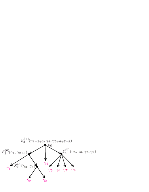
Figure 1: An example of Schröder tree contributing to $\mathscr{R}_{8}$. Near each vertex we showed the corresponding factor using the shorthand notation $\gamma_{i+j}=\gamma_{i}+\gamma_{j}$.

It remains to provide the functions $\mathscr{E}_{n}$. They are given by

$$\mathscr{E}_{n}(\{\hat{\gamma}_{i}\},\tau_{2},\beta)=\Phi^{E}_{n-1}(\{{\boldsymbol{v}}_{\ell}(J)\};{\boldsymbol{x}}),$$ (D.3)

where $\Phi^{E}_{n-1}$ are (boosted) generalized error functions described in appendix C, which depend on $nb_{2}$-dimensional vectors with the following components

$$\begin{split}{\boldsymbol{x}}_{i}^{\alpha}=&\,\sqrt{2\tau_{2}}\left(\tfrac{1}{N_{i}}\,C^{\alpha\beta}q_{i,\beta}+\beta\mathscr{N}_{i}c_{1}^{\alpha}\right),\qquad i=1,\dots,n,\\ {\boldsymbol{v}}_{\ell,i}^{\alpha}(J)=&\,\left(M_{\ell}\delta_{i>\ell}-(N-M_{\ell})\delta_{i\leq\ell}\right)J^{\alpha},\qquad\ell=1,\dots,n-1,\end{split}$$ (D.4)

where $M_{\ell}=\sum_{k=1}^{\ell}N_{k}$ and $\mathscr{N}_{i}=\sum_{j<i}N_{j}-\sum_{j>i}N_{j}$.

The meaning of the vectors (D.4) can be understood as follows. The first vector ${\boldsymbol{x}}$ simply combines all charges $q_{i}$ into one vector and has the form (C.3) required by modularity. This follows from the identity

$$\sum_{i<j}\gamma_{ij}(c_{1})=c_{1}\cdot\sum\limits_{i=1}^{n}\mathscr{N}_{i}q_{i}=\boldsymbol{\mathfrak{p}}{\scriptstyle\boldsymbol{*}}{\boldsymbol{q}},$$ (D.5)

where we introduced the vectors

$$\boldsymbol{\mathfrak{p}}_{i}^{\alpha}=\mathscr{N}_{i}c_{1}^{\alpha},\qquad{\boldsymbol{q}}_{i}^{\alpha}=\tfrac{1}{N_{i}}\,C^{\alpha\beta}q_{i,\beta}$$ (D.6)

and the bilinear form

$${\boldsymbol{x}}{\scriptstyle\boldsymbol{*}}{\boldsymbol{y}}=\sum_{i=1}^{n}N_{i}\,x_{i}\cdot y_{i}.$$ (D.7)

The second vector is designed so that

$${\boldsymbol{v}}_{k}(J)\,{\scriptstyle\boldsymbol{*}}\,{\boldsymbol{x}}=\sqrt{2\tau_{2}}\,\Bigl{(}\Gamma_{k}(J)+\beta NM_{k}(N-M_{k})\,J\cdot c_{1}\Bigr{)}.$$ (D.8)

The first term is nothing but the quantity introduced in (2.18) and appearing as the argument of one set of sign functions in the kernel (2.16) defining the generating functions. Note also that the second set of sign functions in (2.16) can be obtained in a similar way, namely

$${\boldsymbol{w}}_{k,k+1}{\scriptstyle\boldsymbol{*}}\,{\boldsymbol{x}}=\sqrt{2\tau_{2}}\,\mathscr{B}_{k},\qquad{\boldsymbol{w}}_{k\ell,i}^{\alpha}=\left(N_{k}\delta_{i\ell}-N_{\ell}\delta_{ik}\right)v_{0}^{\alpha}.$$ (D.9)

The difference however is that in the first set the $\beta$-dependent shift present in (D.8) disappears. This is because this set as well as the special treatment of vanishing arguments originates in $\mathscr{E}^{(0)}_{n}$. Indeed, evaluating the limit in (D.2), one reproduces the $v_{0}$-independent term in the kernel (2.16) [7]:

$$\mathscr{E}^{(0)}_{n}(\{\hat{\gamma}_{i}\})=\sum_{\mathcal{J}\subseteq\mathscr{Z}_{n-1}}e_{|\mathcal{J}|}\,\delta_{\mathcal{J}}(v)\prod_{k\in\mathscr{Z}_{n-1}\setminus\mathcal{J}}\mbox{\rm sgn}(\Gamma_{k}(J))\,.$$ (D.10)

References

- [1] C. Vafa and E. Witten, “A Strong coupling test of S duality,” Nucl.Phys. B431 (1994) 3–77, hep-th/9408074.
- [2] S. Zwegers, “Mock theta functions.” PhD dissertation, Utrecht University, 2002.
- [3] D. Zagier, “Ramanujan’s mock theta functions and their applications (after Zwegers and Ono-Bringmann),” Astérisque (2009), no. 326, Exp. No. 986, vii–viii, 143–164 (2010). Séminaire Bourbaki. Vol. 2007/2008.
- [4] C. Montonen and D. I. Olive, “Magnetic Monopoles as Gauge Particles?,” Phys. Lett. B 72 (1977) 117–120.
- [5] J. A. Minahan, D. Nemeschansky, C. Vafa, and N. P. Warner, “E strings and N=4 topological Yang-Mills theories,” Nucl. Phys. B527 (1998) 581–623, hep-th/9802168.
- [6] S. Alexandrov and B. Pioline, “Black holes and higher depth mock modular forms,” Comm. Math. Phys. (2019) 1808.08479.
- [7] S. Alexandrov, J. Manschot, and B. Pioline, “S-duality and refined BPS indices,” 1910.03098.
- [8] J. M. Maldacena, A. Strominger, and E. Witten, “Black hole entropy in M-theory,” JHEP 12 (1997) 002, hep-th/9711053.
- [9] D. Gaiotto, A. Strominger, and X. Yin, “New connections between 4d and 5d black holes,” JHEP 02 (2006) 024, hep-th/0503217.
- [10] J. de Boer, M. C. N. Cheng, R. Dijkgraaf, J. Manschot, and E. Verlinde, “A farey tail for attractor black holes,” JHEP 11 (2006) 024, hep-th/0608059.
- [11] S. Alexandrov, S. Banerjee, J. Manschot, and B. Pioline, “Multiple D3-instantons and mock modular forms I,” Commun. Math. Phys. 353 (2017), no. 1, 379–411, 1605.05945.
- [12] S. Alexandrov, B. Pioline, F. Saueressig, and S. Vandoren, “D-instantons and twistors,” JHEP 03 (2009) 044, 0812.4219.
- [13] S. Alexandrov, “D-instantons and twistors: some exact results,” J. Phys. A42 (2009) 335402, 0902.2761.
- [14] S. Alexandrov and B. Pioline, “S-duality in Twistor Space,” JHEP 1208 (2012) 112, 1206.1341.
- [15] S. Alexandrov, J. Manschot, and B. Pioline, “D3-instantons, Mock Theta Series and Twistors,” JHEP 1304 (2013) 002, 1207.1109.
- [16] S. Alexandrov, “Twistor Approach to String Compactifications: a Review,” Phys.Rept. 522 (2013) 1–57, 1111.2892.
- [17] S. Alexandrov, J. Manschot, D. Persson, and B. Pioline, “Quantum hypermultiplet moduli spaces in N=2 string vacua: a review,” in Proceedings, String-Math 2012, Bonn, Germany, July 16-21, 2012, pp. 181–212. 2013. 1304.0766.
- [18] K. Bringmann, J. Kaszian, and A. Milas, “Higher depth quantum modular forms, multiple Eichler integrals, and false theta functions,” Res. Math. Sci. 6 (2017) 20, 1704.06891.
- [19] A. Dabholkar, P. Putrov, and E. Witten, “Duality and Mock Modularity,” 2004.14387.
- [20] M.-x. Huang, S. Katz, and A. Klemm, “Topological String on elliptic CY 3-folds and the ring of Jacobi forms,” JHEP 10 (2015) 125, 1501.04891.
- [21] J. Gu, M.-x. Huang, A.-K. Kashani-Poor, and A. Klemm, “Refined BPS invariants of 6d SCFTs from anomalies and modularity,” JHEP 05 (2017) 130, 1701.00764.
- [22] S. Alexandrov, “Vafa-Witten invariants from modular anomaly,” 2005.03680.
- [23] K. Yoshioka, “The Betti numbers of the moduli space of stable sheaves of rank 2 on a ruled surface,” Mathematische Annalen 302 (1995) 519–540.
- [24] K. Yoshioka, “Euler characteristics of instanton moduli spaces on rational elliptic surfaces,” Commun. Math. Phys. 205 (1999), no. 3, 501–517.
- [25] J. Manschot, “BPS invariants of N=4 gauge theory on Hirzebruch surfaces,” Commun. Num. Theor. Phys. 06 (2012) 497–516, 1103.0012.
- [26] J. Manschot, “BPS invariants of semi-stable sheaves on rational surfaces,” Lett. Math. Phys. 103 (2013) 895–918, 1109.4861.
- [27] A. Klemm, J. Manschot, and T. Wotschke, “Quantum geometry of elliptic Calabi-Yau manifolds,” Comm. Number Theor. Phys. 6 (2012) 849–917, 1205.1795.
- [28] G. Beaujard, J. Manschot, and B. Pioline, “Vafa-Witten invariants from exceptional collections,” 2004.14466.
- [29] M. Kontsevich and Y. Soibelman, “Stability structures, motivic Donaldson-Thomas invariants and cluster transformations,” 0811.2435.
- [30] D. Joyce and Y. Song, “A theory of generalized Donaldson-Thomas invariants,” Memoirs of the Am. Math. Soc. 217 (2012), no. 1020, 0810.5645.
- [31] D. Joyce, “Generalized Donaldson-Thomas invariants,” Surveys in differential geometry 16 (2011), no. 1, 125–160, 0910.0105.
- [32] K. Yoshioka, “The chamber structure of polarizations and the moduli of stable sheaves on a ruled surface,” Int. J. of Math. 7 (1996) 411–431, 9409008.
- [33] L. Göttsche, “Theta functions and Hodge numbers of moduli spaces of sheaves on rational surfaces,” Commun. Math. Phys. 206 (1999), no. 1, 105–136, 9808007.
- [34] W.-P. Li and Z.-b. Qin, “On blowup formulae for the S duality conjecture of Vafa and Witten,” Invent. Math. 136 (1999) 451, math/9805054.
- [35] D. Joyce, “Configurations in abelian categories. iv. invariants and changing stability conditions,” Advances in Mathematics 217 (2008), no. 1, 125–204.
- [36] J. Manschot, “Sheaves on and generalized Appell functions,” Adv. Theor. Math. Phys. 21 (2017) 655–681, 1407.7785.
- [37] K. Yoshioka, “The Betti numbers of the moduli space of stable sheaves of rank 2 on ,” J. Reine Angew. Math 453 (1994) 193–220.
- [38] J. Manschot, “The Betti numbers of the moduli space of stable sheaves of rank 3 on ,” Lett.Math.Phys. 98 (2011) 65–78, 1009.1775.
- [39] S. Alexandrov, S. Banerjee, J. Manschot, and B. Pioline, “Indefinite theta series and generalized error functions,” Selecta Mathematica 24 (2018) 3927–3972, 1606.05495.
- [40] J. Manschot, “Vafa-Witten theory and iterated integrals of modular forms,” Comm. Math. Physics (2019) 1709.10098.
- [41] J. Manschot, “Wall-crossing of D4-branes using flow trees,” Adv.Theor.Math.Phys. 15 (2011) 1–42, 1003.1570.
- [42] L. Göttsche, “The Betti numbers of the Hilbert scheme of points on a smooth projective surface,” Math. Ann. 286 (1990) 193–207.
- [43] S. Alexandrov and B. Pioline, “Attractor flow trees, BPS indices and quivers,” Adv. Theor. Math. Phys. 23 (2019), no. 3, 627–699, 1804.06928.
- [44] F. Denef and G. W. Moore, “Split states, entropy enigmas, holes and halos,” JHEP 1111 (2011) 129, hep-th/0702146.
- [45] I. Bena, M. Berkooz, J. de Boer, S. El-Showk, and D. Van den Bleeken, “Scaling BPS Solutions and pure-Higgs States,” JHEP 1211 (2012) 171, 1205.5023.
- [46] M. Eichler and D. Zagier, The theory of Jacobi forms, vol. 55 of Progress in Mathematics. Birkhäuser Boston Inc., Boston, MA, 1985.
- [47] C. Nazaroglu, “-Tuple Error Functions and Indefinite Theta Series of Higher-Depth,” Commun. Num. Theor. Phys. 12 (2018) 581–608, 1609.01224.
- [48] S. Alexandrov, S. Banerjee, J. Manschot, and B. Pioline, “Multiple D3-instantons and mock modular forms II,” Commun. Math. Phys. 359 (2018), no. 1, 297–346, 1702.05497.
- [49] K. Bringmann, J. Manschot, and L. Rolen, “Identities for Generalized Appell Functions and the Blow-up Formula,” Lett. Math. Phys. 106 (2016) 1379–1395, 1510.00630.
- [50] J. Conway and M. Sloane, Sphere packings, lattices and groups. Springer, 1999.
- [51] S. Mozgovoy, “Invariants of moduli spaces of stable sheaves on ruled surfaces,” 1302.4134.