On the Effects of Pointing Jitter, Actuators Drift, Telescope Rolls and Broadband Detectors in Dark Hole Maintenance and Electric Field Order Reduction

Abstract

Space coronagraphs are projected to detect exoplantes that are at least $10^{10}$ times dimmer than their host stars. Yet, the actual detection threshold depends on the instrument’s wavefront stability and varies by an order of magnitude with the choice of observation strategy and post-processing method. In this paper the authors consider the performance of the previously introduced observation strategy (dark hole maintenance) and post-processing algorithm (electric field order reduction) in the presence of various realistic effects. In particular, it will be shown that under some common assumptions, the telescope’s averaged pointing jitter translates into an additional light source incoherent with the residual light from the star (speckles), and that jitter “modes” can be identified in post-processing and distinguished from a planet signal. We also show that the decrease in contrast due to drift of voltages in deformable mirror actuators can be mitigated by recursive estimation of the electric field in the high-contrast region of the image (dark hole) using Electric Field Conjugation (EFC). Moreover, this can be done even when the measured intensity is broadband, as long as it is well approximated by an incoherent sum of monochromatic intensities. Finally, we assess the performance of closed-loop vs. open-loop observation scenarios through a numerical simulation of the Wide-Field Infra-Red Survey Telescope (WFIRST). In particular, we compare the post-processing factors of Angular Differential Imaging (ADI) with and without Electric Field Order Reduction (EFOR), which we extended to account for possible telescope rolls and the presence of pointing jitter. For all observation parameters considered in this paper, close-loop dark hole maintenance resulted in significantly higher post-processing accuracy.

*Leonid Pogorelyuk, leonidp@princeton.edu

1 Introduction

1.1 Context

Future space coronagraphs are projected to detect tens of exo-earths that are $10^{10}$ times dimmer than their host stars.[1] Contrasts of better than $4\cdot 10^{-10}$ have already been demonstrated in the lab[2] in preparation for the WFIRST mission[3, 4]. Such high contrasts are unlikely to persist on their own throughout lengthy observations (tens of hours required to achieve a reasonable signal-to-noise ratio (S/N) to detect a Jupiter-like planet[5]), due to thermal and structural instabilities[6]. As an example, the wavefront error budget for the quadrafoil error (4th Zernike mode) is on the order of $0.1\>\mathrm{nm}$ for WFIRST[7], and would be even lower for future missions[8] such as the Habitable Exoplanet Imaging Mission (HabEx)[9] and Large UV/Optical/IR Surveyor (LUVOIR)[10].

A potentially major source of instabilities are telescope maneuvers. The proposed WFIRST observation scenario will keep the Deformable Mirrors (DMs) fixed for 8 hour long exposures followed by a 2 hour long dark hole “re-creation” procedure while pointing at a reference star[11]. The electric field of the speckles will be estimated and reduced via pair-probing and Electic Field Conjugation (EFC)[12, 13] based on narrowband intensity measurement (either using an Integral Field Spectrometer (IFS) or sequentially, using multiple narrowband filters). This results in a sawtooth temporal pattern for the contrast (see Figs.  15,16 in [14]) with “spikes” due to increased pointing jitter after the telescope “switches” back from the reference star.

An alternative approach (proposed by the authors in Ref. 15) is to maintain the contrast in the dark hole throughout the observation in a closed-loop fashion. In section 2, we extend this method to work with broadband intensity measurements, illustrate how it handles pointing jitter (residual errors from fast-steering mirrors[16]) and drift of the DM actuators[17]. The results are numerically compared to the WFIRST observation scenario.

The authors have also previously suggested that known DM perturbations introduced during a closed-loop observation phase can be exploited in post-processing. In section 3, we extend Electric Field Order Reduction (EFOR[18]) to incorporate images taken at different telescope orientations and subtracts the contribution of the jitter (by identifying a small number of fast-varying jitter modes). We then estimate the post-processing errors associated with open- and closed-loop observations, EFOR and Angular Differential Imaging (ADI [19, 20]).

The numerical results in sections 2 and 3 suggest that dark hole maintenance increases the average contrast regardless of the nature of the drift, presence or absence of jitter and measurement type (monochromatic or broadband). Consequently, the planet detection thresholds are lower for data obtained in closed-loop scenarios, although the best choice of post-processing method depends on the parameters of the observation.

1.2 Notations

To generalize the discussion to both monochromatic and broadband light, we discretize the time depended electric field of the speckles in the high-contrast region of the image (the dark hole), $E(t,\mathbf{x},\lambda)$, based on location, $\mathbf{x}$, and wavelength, $\lambda$ (similarly to the formulation in Ref. 18). In other words, the electric field in the focal plane will be modelled as

$$\mathbf{E}(t)=\begin{bmatrix}\mathrm{Re}\left\{E(t,\mathbf{x}_{1},\lambda_{1})\right\}\\ \mathrm{Im}\left\{E(t,\mathbf{x}_{1},\lambda_{1})\right\}\\ \mathrm{Re}\left\{E(t,\mathbf{x}_{1},\lambda_{2})\right\}\\ \mathrm{Im}\left\{E(t,\mathbf{x}_{1},\lambda_{2})\right\}\\ \vdots\end{bmatrix}\in\mathbb{R}^{2nl}$$ (1)

where $\mathbf{x}_{p},\>1\leq p\leq n$ are the centers of the $n$ pixels in the dark hole and $\lambda_{q},\>1\leq q\leq l$ is some discretization of the spectrum. The intensity of the speckles at the detectors is therefore given by

$$\mathbf{I}(t)=B\cdot\left(\mathbf{E}(t)\circ\mathbf{E}(t)\right)\in\mathbb{R}^{nm},$$ (2)

where $\circ$ stands for the Hadamard product, $m$ is the number of channels in the detector and $B\in\mathbb{R}^{nm\times 2nl}$ is the linear operator for summing the real and imaginary parts of all wavelengths in a channel (for broadband light, $l>1$, and for a single channel detector, $m=1$, it is given by the Kronecker product of the identity matrix and a row vector of ones, $B=I_{n\times n}\otimes\mathbf{1}_{2l}^{T}$).

2 Dark Hole Maintenance

Coronagraphs use DMs to achieve a high initial contrast, for example, by measuring the focal plane intensity with different control settings (probes [12]), estimating the electric field and applying corrections[13]. Most such approaches[21] do not incorporate a noise model and therefore become extremely inaccurate when pointing at a dim star since the number of photons detected per observation frame is of order 1 (and so is the noise variance). In contrast, recursive estimation via the Extended Kalman Fitler (EKF)[22], incorporates all prior measurement and gives the appropriate weight to the new noisy observations. It allows observing a dim target star while maintaining contrast only slightly lower than in a “perfect” dark hole[15]. Below we formulate the EKF for the general spectrum discretization, eqs. (1)-(2), and address the effects of pointing jitter and DM actuators drift.

2.1 Appearance of Pointing Jitter

The pointing jitter due to telescope reaction wheels is mostly compensated for by fast-steering mirrors (FSMs), but the residual wavefront perturbations are non-negligible[16]. Unlike fluctuations in structural modes, their timescale is much shorter than a single exposure; hence, they cannot be temporally resolved. Instead, one has to consider their averaged contribution to incoherent sources and assume that it varies slowly across multiple frames.

We begin by splitting the temporal variations of the electric field of the speckles into their average and zero mean components during each observation frame $k$,

$$\mathbf{E}(t)=\left\langle\mathbf{E}\right\rangle(k)+\delta\mathbf{E}(t),\>t\in\left[t_{k},t_{k+1}\right),$$ (3)

where $\left\langle\cdot\right\rangle(k)$ denotes averaging over $\left[t_{k},t_{k+1}\right)$ and $\left\langle\delta\mathbf{E}\right\rangle(k)=\mathbf{0}$. We further denote the sensitivity of the field to small control actuations, $\mathbf{u}$, as the Jacobian $G^{U}=\partial\mathbf{E}/\partial\mathbf{u}$, and define the “open-loop electric field” as

$$\mathbf{E}^{OL}(k)\equiv\left\langle\mathbf{E}\right\rangle(k)-G^{U}\mathbf{u}(k).$$ (4)

In a perfectly linear model, $\mathbf{E}^{OL}(k)$ would be the average electric field (including FSM corrections) if the DMs were kept fixed ($\mathbf{u}(k)=0$) after the dark hole has been created.

The average speckle intensity, $\left\langle\mathbf{I}\right\rangle(k)$, can be shown to have two components,

$$\left\langle\mathbf{I}\right\rangle(k) =\mathbf{I}^{S}(k)+\mathbf{I}^{J}(k),$$ (5)

$$\mathbf{I}^{S}(k) =B\cdot\left(\mathbf{E}^{OL}(k)+G^{U}\mathbf{u}(k)\right)^{\circ 2},$$ (6)

$$\mathbf{I}^{J}(k) =\left\langle B\cdot\left(\delta\mathbf{E}(t)\right)^{\circ 2}\right\rangle(k).$$ (7)

Here $\mathbf{I}^{S}(k)$ captures (mostly) the variations of the speckles due to “slow” thermal and structural instabilities, while $\mathbf{I}^{J}(k)$ is mostly due to jitter (the time average of the cross term $\left(\mathbf{E}^{OL}(k)+G^{U}\mathbf{u}(k)\right)\circ\delta\mathbf{E}(t)$ is zero). The total intensity, $\mathbf{I}$, also includes sources incoherent with the star, $\mathbf{I}^{I}$, and detector noise sources, $\mathbf{I}^{D}$ (e.g. dark current),

$$\mathbf{I}=\mathbf{I}^{S}+\mathbf{I}^{J}+\mathbf{I}^{I}+\mathbf{I}^{D}.$$ (8)

It is now evident that the fast variations in the electric field due to jitter resemble other incoherent sources in the sense that they remain almost unaffected by slow variations in high-order wavefront errors and DM commands. Differentiating between jitter and other incoherent sources is done in post-processing (Sec. 3.1) while the algorithm below allows for a reduction in the intensity of the speckles, $\mathbf{I}^{S}$—the only source affected by the DMs.

2.2 Broadband Extended Kalman Filter

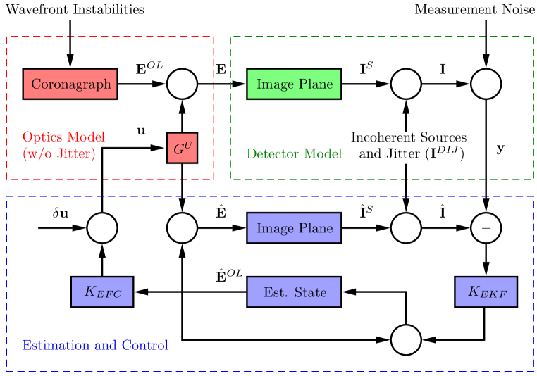
Figure 1: A diagram of the linearized model of the coronagraph with jitter contribution approximated by an incoherent light source. The top half of this figure describes how the actual instrument hardware is simulated in this paper while the bottom half illustrates the main functionalities of the Dark hole maintenance algorithm.

We are interested in efficiently computing a rough estimate of the slowly varying open-loop electric field, $\hat{\mathbf{E}}^{OL}$, in order to apply corrections to the DMs,

$$\mathbf{u}(k)=-K_{EFC}\hat{\mathbf{E}}^{OL}(k-1)+\delta\mathbf{u}(k),$$ (9)

where $K_{EFC}$ is the EFC gain[13], and $\delta\mathbf{u}(k)$ is random DM dither (Fig. 1). Note that the mean component of the jitter is already included in $\mathbf{E}^{OL}$ and we further assume that “variance” of the jitter, $\mathbf{I}^{J}(k)$, changes slowly between frames. We may therefore gather the terms in Eq. (8) which are unaffected by controls

$$\mathbf{I}(k)=\mathbf{I}^{S}(k)+\mathbf{I}^{DIJ}(k),$$ (10)

and apply the existing EKF algorithm for estimating both $\mathbf{E}^{OL}(k)$ and $\mathbf{I}^{DIJ}(k)$ without modifications (see Appendix A in Ref. 15). However, since the variations in the residual pointing jitter are very small, the authors found $\mathbf{I}^{DIJ}\approx\mathrm{const}$ to be empirically justifiable as it reduces the dimension of the EKF, making it more tractable without compromising its accuracy.

Another simplification, for numerical purposes, consists of ignoring the correlation of electric field increments between pixels. We assume that they are normally distributed with zero mean and a block diagonal covariance matrix, $\Sigma$,

$$\mathbf{E}^{OL}(k)-\mathbf{E}^{OL}(k-1)\sim{\cal N}\left(\mathbf{0},\Sigma\right).$$ (11)

Ignoring the dependence between pixels (by discarding the off-diagonal terms in $\Sigma$) greatly reduces the accuracy of the filter but allows propagating all the estimates in ${\cal O}(n)$ operations per frame instead of the ${\cal O}(n^{3}$) required for the full EKF (it is possible to exploit the low-order nature of the electric field increments to recover some of the information while keeping an ${\cal O}(n)$ complexity[23]).

The EKF is formulated in terms of the open-loop electric field estimates, $\hat{\mathbf{E}}^{OL}(k)$. It is advanced based on the the number of photons detected in the physical system, $\mathbf{y}(k)$, which presumably follows a multivariate Poisson distribution parameterized by the intensity, $\mathbf{I}(k)$. For estimation purposes, it is approximated by a normal distribution with mean and variance both equal to the intensity estimate, $\mathbf{\hat{\mathbf{I}}}$, at step $k$,

$$\mathbf{y}(k) \sim{\cal N}\left(\hat{\mathbf{I}}(k),\mathrm{diag}\left(\hat{\mathbf{I}}(k)\right)\right),$$ (12)

$$\hat{\mathbf{I}}(k) =B\cdot\left(\hat{\mathbf{E}}^{OL}(k)+G^{U}\mathbf{u}(k)\right)^{\circ 2}+\mathbf{I}^{DIJ},$$ (13)

where $\mathrm{diag}(\mathbf{a})$ stands for a diagonal matrix with the elements of $\mathbf{a}$ on its diagonal.

Apart from the shot noise, which has an estimated covariance of $\mathrm{diag}\left(\hat{\mathbf{I}}(k)\right)$, the uncertainty in the state estimate, $\hat{\mathbf{E}}^{OL}(k)-\mathbf{E}^{OL}(k)$, also has a covariance, $P(k)$, which needs to be accounted for. The two are combined in the EKF gain given by

$$K_{EKF}(k)=P(k)H^{T}(k)\left(H(k)P(k)H^{T}(k)+\mathrm{diag}\left(\hat{\mathbf{I}}(k)\right)\right)^{-1},$$ (14)

where $H(k)$ denotes the linearized effect of the open-loop electric field on the measurements,

$$H(k)=\frac{\partial\hat{\mathbf{I}}(k)}{\partial\hat{\mathbf{E}}^{OL}(k)}=2B\cdot\mathrm{diag}\left(\hat{\mathbf{E}}^{OL}(k)+G^{U}\mathbf{u}(k)\right).$$ (15)

Note that the last equation requires that both $\mathbf{u}(k)$ and $\hat{\mathbf{E}}^{OL}(k)-\mathbf{E}^{OL}(k)$ be small, so that the coronagraph is in the linear regime and the EKF gain is “roughly in the correct direction”.

The above gain is used to advance the estimated state based on the discrepancy between the predicted measurement, $\hat{\mathbf{I}}(k)$, and the actual one, $\mathbf{y}(k)$, (the innovation),

$$\hat{\mathbf{E}}^{OL}(k+1)=\hat{\mathbf{E}}^{OL}(k)+K_{EKF}(k)\left(\mathbf{y}(k)-\hat{\mathbf{I}}(k)\right).$$ (16)

As a result, the gain acts to decrease the error covariance, $P$, which would otherwise be constantly increasing due to unknown drift increments (with covariance $\Sigma$). Both of these effects are accounted for when advancing the covariance matrix approximation,

$$P(k+1)=\left(I-K_{EKF}(k)H(k)\right)P(k)+\Sigma.$$ (17)

Since we ignore the cross-correlation between pixels, the matrices $P,R,H$ and $\Sigma$ are block diagonal. Taking advantage of that, the EKF can be advanced independently for each pixel giving an ${\cal O}(n)$ time and space complexity for all the pixels combined. We also note that the spectral discretization in the above formulation is implicit in the dimensions of $\mathbf{y}$, $\hat{\mathbf{E}}$ and the elements of $B$. Hence, it applies to both to single- ($l>m=1$) and multi- channel ($l\geq m>1$) detectors. Finally, we require that the magnitude (covariance) of the dither, $\delta\mathbf{u}$, is comparable to $\Sigma$ (although its exact distribution is not important if it is random).

2.3 The Effect of DM Actuators Drift

In a realistic scenario, the actual DM actuations, $\mathbf{u}_{true}(k)$, might slightly differ from the deterministic commands, $\mathbf{u}(k)$[17]. If left unchecked, these DM surface discrepancies might result in an unwanted intensity buildup.

For lack of a better model, we assume that the time-evolution of the difference between prescribed and actual commands, i.e., the DM drift, can be approximated by a random walk of a known magnitude, $\sigma_{a}$,

$$\mathbf{u}_{true}(k) =\mathbf{u}(k)+\mathbf{u}_{drift}(k),$$ (18)

$$\mathbf{u}_{drift}(k+1)-\mathbf{u}_{drift}(k) \sim{\cal N}\left(\mathbf{0},\sigma_{a}^{2}I\right).$$ (19)

Given the definition of the open-loop electric field, (4), we observe that the only implication of the DM drift is the increase in the covariance of the electric field increments, and in particular

$$\mathrm{cov}\left\{\mathbf{E}^{OL}(k+1)-\mathbf{E}^{OL}(k)\right\}\geq\sigma_{a}^{2}G^{U}\left(G^{U}\right)^{T}.$$ (20)

While the EKF in eqs. (13)-(15) remain unchanged (regardless of whether the actuators are statistically independent or not), the full drift covariance and its block diagonal approximation, $\Sigma$, have to be increased to account for this additional source of uncertainty. It’s worth noting that the accuracy of the filter is not very sensitive to the exact values of the elements of $\Sigma$.

2.4 Numerical Results

To assess the performance of the dark hole maintenance scheme[15] in the presence of the above mentioned effects, the authors employed the FALCO[24] model of the WFIRST Hybrid Lyot Coronagraph. The simulations consisted of series of 5 single wavelength images equally spaced between $546\>\mathrm{nm}$ and $601\>\mathrm{nm}$. The initial dark hole had a contrast of $4.2\cdot 10^{-10}$ in a ring between $3$ and $9$ $\lambda/D$ with an average flux of $1.2\>\frac{\mathrm{\mathrm{photon}}}{\mathrm{frame}}$ (per pixel and wavelength) from the star and $0.25\>\frac{\mathrm{\mathrm{photon}}}{\mathrm{frame}}$ from dark current. This slowly-varying speckle drift was simulated via random walk of the first $21$ Zernike polynomials (denoted by their time averages within each frame),

$$\left\langle z_{p}^{p-2j}\right\rangle(k+1)-\left\langle z_{p}^{p-2j}\right\rangle(k)\sim{\cal N}\left(0,\left(\frac{\sigma_{d}}{(p+1)^{2}\cdot\lambda}\right)^{2}\Delta t\right),\;0\leq j\leq p$$ (21)

where $p$ is the order of the polynomial, $j$ is its azimuthal degree, $\Delta z_{p}^{p-2j}$ is its increment over one $\Delta t=100\>\mathrm{sec}$ frame, and $\sigma_{d}=0.2\>\frac{\mathrm{nm}}{\sqrt{\mathrm{hr}}}$. The pointing jitter in the simulation can be described as fast periodic perturbations of the the tip/tilt Zernikes, $z_{\mathrm{tip/tilt}}=z_{1}^{\pm 1}$,

$$z_{\mathrm{tip}}(t)-\left\langle z_{\mathrm{tip}}\right\rangle(k+1) =a_{\mathrm{tip}}(k)\sin\left(\frac{2\pi}{\Delta t}t\right),\>t\in\left[t_{k},t_{k+1}\right),$$ (22)

$$z_{\mathrm{tilt}}(t)-\left\langle z_{\mathrm{tilt}}\right\rangle(k+1) =a_{\mathrm{tilt}}(k)\sin\left(\frac{2\pi}{\Delta t}t+\phi_{k}\right),\>t\in\left[t_{k},t_{k+1}\right),$$ (23)

where $a_{\mathrm{tip/tilt}}(k)$ varied slowly throughout the simulation between $0$ and $1.4\>\mathrm{nm}$ and $\phi_{k}$ between $0$ and $2\pi$ (the added intensity was computed by analytically averaging Eq. (7)).

The closed loop control law in Eq. (9) was applied with $\delta\mathbf{u}(k)\sim{\cal N}\left(\mathbf{0},\sigma_{u}^{2}I\right)$ and $\sigma_{u}=5-10\>\mathrm{mV}$ (this dither introduces phase diversity and keeps the EKF stable and its optimal magnitude depends on the drift rate). While the above control command was “passed” to the EKF, the actual DM command used for the simulation also included actuators drift with $\sigma_{a}=5\>\frac{\mathrm{mV}}{\sqrt{\mathrm{hr}}}$ as described in eqs. (18)-(19) (this value was chosen such that DM and wavefront drift effects are of the same order).

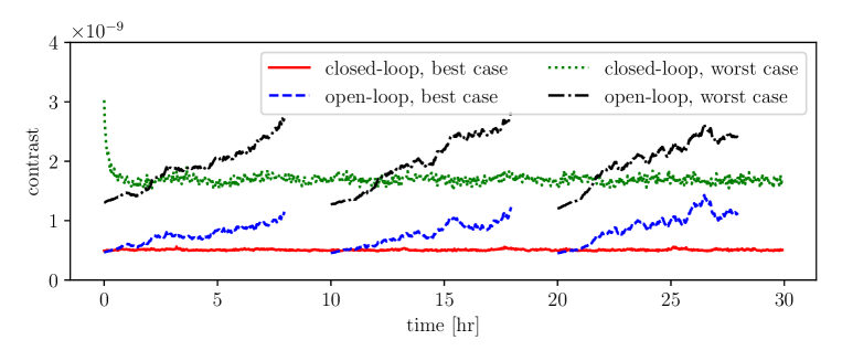
Figure 2: Dark hole maintenance[15] in the presence of realistic effects (dotted green line) and its comparison to an open loop observation with periodic re-creation of the dark hole (dash-dotted black). In the best-case scenario (solid red and dashed blue), only Zernike drift was present and the five narrowband channels were available separately for the EKF. In the worst-case scenario (dotted green and dash-dotted black), Zernikes, DM actuators drift and pointing jitter were present and just one broadband channel was used by the EKF. As a result, the dither necessary to keep the EKF stable was higher and the contrast was worse.

Fig. 2 compares the dark hole maintenance (closed-loop) scheme with the proposed WFIRST-CGI open-loop observation scenario which requires periodically observing a reference star to re-create the dark hole[11] (hence the missing two-hour segments in the open-loop lines). When only Zernikes drift was simulated and all five channels were available for the EKF (best case), a small dither magnitude, $\sigma_{u}=5\>\mathrm{mV}$, was sufficient to maintain the contrast at almost its initial level. When DM drift and jitter were present (worst case), the initial contrast was lower and the open-loop contrast decreased significantly faster. Additionally, the EKF had access to just the sum of all the channels, hence a larger dither magnitude, $\sigma_{u}=10\>\mathrm{mV}$, was necessary to ensure stability, it took more time to converge and the closed loop contrast varied slightly with the jitter magnitude (dotted green line).

In all cases, the closed-loop approach maintained a significantly higher contrast throughout most of the observation, compared to the open-loop observation scenario. Besides utilizing close to 100% of the duty cycle, closing the loop also avoids telescope pointing maneuvers which might excite structural modes and decrease the open-loop contrast further (not simulated here).

Another potential benefit of closed-loop observations manifests itself in post-processing. While DM dithering was introduced to stabilize the EKF, it also provides phase diversity which helps to detect faint sources below the speckle floor. This is a non-linear and computationally expensive procedure, but it also allows accounting for the low-dimensionality of the speckles and telescope rolls as discussed in the next section.

2.5 Dark Hole Creation with Broadband Measurements

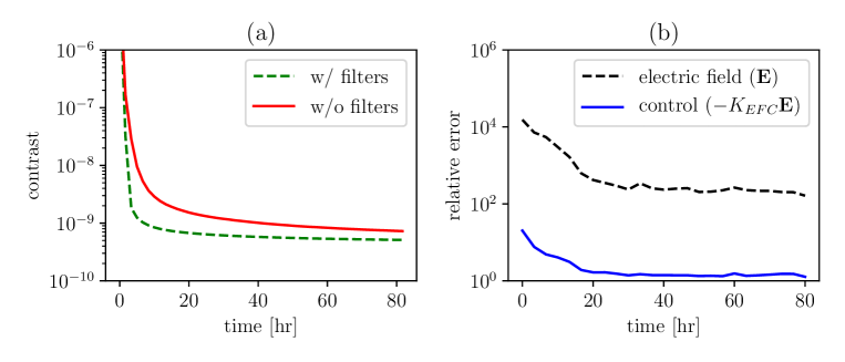
Figure 3: (a) Contrast evolution during the creation of the dark hole with pair-probing and EFC. When monochromatic intensities where measured sequentially (using optical filters, dashed green line), the contrast increased faster than when the all measurements were broadband (without filters, solid red line). (b) The relative errors in the electric field estimate (dashed black line) and the corresponding EFC correction (solid blue line), both based on broadband measurements. The ambiguities involved in estimating spectral information from broadband measurements are “cancelled out” by the EFC gain for reasons discussed in Appendix A.

In the “closed-loop worst-case” simulation in figure 2, the contrast was maintained with focal-plane broadband measurements alone. This suggests that it could also be possible to create the dark hole without an IFS or optical filters. Indeed, the pair-probing approach[12] for estimating the electric field can be modified slightly to include broadband measurements, and the EFC control law for increasing the contrast is already “broadband”.

The goal of pair-probing is to estimate the electric field in the dark hole, $\mathbf{E}^{DH}$, by measuring the effects of $2s$ DM probes $\left\{\pm\delta\mathbf{u}_{j}\right\}_{j=1}^{s}$on the intensity, $\mathbf{I}^{DH}$. It is assumed that the intensity measurements have a high S/N and that the speckles and incoherent sources do not drift during the “probing”. With the generalized spectral discretization in Eq. (1), the (possibly broadband) intensity is given by

$$\mathbf{I}^{DH}(\pm\delta\mathbf{u}_{j})=B\cdot\left(\mathbf{E}^{DH}\pm G^{U}\delta\mathbf{u}_{j}\right)^{\circ 2}+\mathbf{I}^{DIJ},$$ (24)

where $\mathbf{I}^{DIJ}=\mathrm{const}$ is the sum of incoherent sources. It follows that

$$\left(4B\cdot\mathrm{diag}(G^{U}\delta\mathbf{u}_{j})\right)\mathbf{E}^{DH}=\mathbf{I}^{DH}(+\delta\mathbf{u}_{j})-\mathbf{I}^{DH}(-\delta\mathbf{u}_{j}).$$ (25)

Each pair of probes therefore gives $mn$ sparse linear equations in $2nl=\mathrm{dim}\hat{\mathbf{E}}$ unknowns. Picking $s\geq 2nl/m$ probes results in a least-squares problem for estimating $\mathbf{E}^{DH}$,

$$\begin{bmatrix}4B\cdot\mathrm{diag}(G^{U}\delta\mathbf{u}_{1})\\ \vdots\\ 4B\cdot\mathrm{diag}(G^{U}\delta\mathbf{u}_{s})\end{bmatrix}\hat{\mathbf{E}}^{DH}\approx\begin{bmatrix}\mathbf{I}^{DH}(+\delta\mathbf{u}_{1})-\mathbf{I}^{DH}(-\delta\mathbf{u}_{1})\\ \vdots\\ \mathbf{I}^{DH}(+\delta\mathbf{u}_{s})-\mathbf{I}^{DH}(-\delta\mathbf{u}_{s})\end{bmatrix}.$$ (26)

The estimate, $\hat{\mathbf{E}}^{DH}$, is then used with the EFC control law,

$$\Delta\mathbf{u}^{DH}=-K_{EFC}\hat{\mathbf{E}}^{DH},$$ (27)

where $\Delta\mathbf{u}^{DH}$ is the DM correction to be applied before the next iteration of the dark hole creation sequence. Note that the Jacobian, $G^{U}$, and the estimate, $\hat{\mathbf{E}}^{DH}$, contain information about the spectrum while the measurements, $\mathbf{I}^{DH}$, may now contain an arbitrary number of channels.

Figure 3(a) shows a dark hole creation sequence using the same FALCO[24] model of the WFIRST as the previous subsection but slightly different observation parameters: no wavefront drift or jitter and a 16 times brighter “reference” star. The broadband variant of the algorithm, i.e., without optical filters or $m=1$, was able to increase the contrast from $10^{-5}$ to $10^{-9}$. Yet, it converged slower than the algorithm which measured each of the five channels separately, i.e., $m=l=5$ (both variants are described by eqs. (26)-(27) with a different $B$ matrix).

Since the dark holes were created using “random” probes and a fixed EFC gain, the convergence rates in Fig. 3(a) are qualitative. Yet, they demonstrate the feasibility of operating a purely broadband coronagraph while pointing out the advantage of having optical filters.

Arguably, it should be difficult to distinguish between speckles at different wavelengths based on an incoherent sum of of their intensities. To assess the accuracy of the electric field estimates in each wavelength, Fig. 3(b) plots their relative error, $\left\|\mathbf{E}^{DH}-\hat{\mathbf{E}}^{DH}\right\|/\left\|\mathbf{E}^{DH}\right\|$. As it turns out, the errors in $\hat{\mathbf{E}}^{DH}$ are many orders of magnitude larger than the actual electric field, $\mathbf{E}^{DH}$, although they are not propagated to $\Delta\mathbf{u}^{DH}$. In other words, the relative difference between the “perfect” and estimated DM increments, $\left\|K_{EFC}\mathbf{E}^{DH}-K_{EFC}\hat{\mathbf{E}}^{DH}\right\|/\left\|K_{EFC}\mathbf{E}^{DH}\right\|$, is small enough to allow creating the dark hole. This peculiar “error cancelling” is analyzed in Appendix A.

3 Electric Field Order Reduction

The observation scenario proposed for WFIRST-CGI prescribes collecting reference images every ten hours and $\pm 13\>\mathrm{deg}$ telescope rolls every two hours[11]. These maneuvers will be utilized in post-processing via Angular Differential Imaging (ADI)[19, 20] and Reference Differential Imaging (RDI)[25]. The collection of all the reference images could, in theory, produce a library of “most descriptive” speckle patterns which could be projected out of the observation[26, 27, 28]. However, the DM commands will change between the observations (either due to drift or due to dark hole re-creation every ten hours), resulting in temporally varying high-order wavefront aberrations. We expect this to reduce the applicability of reference images between temporally distant observations thus hindering the use of intensity-based order reduction methods.

Another source of phase diversity is provided by the dithering of the DMs during a closed-loop observation (see, Eq. (9)); this can help differentiate between speckles which are affected by the DMs and other intensity sources[15]. However, as discussed in Sec. 2.1, the jitter is not affected by dither and would be indistinguishable from incoherent sources including planets. Nevertheless, the Electric Field Order Reduction (EFOR) method proposed in Ref. 18 makes additional assumptions on the nature of the speckle drift that allow identifying the jitter components in the images. In particular, it assumes that the open-loop electric field lies in a low-dimensional subspace,

$$\mathbf{E}^{OL}=G^{V}\mathbf{v},$$ (28)

where the columns of $G^{V}\in\mathbb{R}^{2nl\times r}$ form a basis of $r$ “significant” electric field modes ($r$ depends on the telescope configuration, e.g. segmented vs. monolithic, and is a tuning parameter that can be optimized[29]). Below we describe EFOR and extend it to account for telescope rolls and identify a small number of the modes in $G^{V}$ as “jitter” modes, thus allowing them to be subtracted from the incoherent signal estimate. Our numerical simulations show that this low-order assumption breaks down if the dominant source of wavefront drift are DM actuators (due to their high spatial frequency), in which case a closed-loop observation scenario with ADI gives the most accurate estimates.

3.1 Pointing Jitter and Telescope Rolls

Similarly to Eq. (3), time variations of speckle modes, $\mathbf{v}$, can be split into their average, $\left\langle\mathbf{v}\right\rangle$, and zero mean, $\delta\mathbf{v}$, components,

$$\mathbf{v}(t)=\left\langle\mathbf{v}\right\rangle(k)+\delta\mathbf{v}(t),\>t\in\left[t_{k},t_{k+1}\right).$$ (29)

Consequently, the jitter term defined in Eq. (7) becomes

$$\mathbf{I}^{J}(k)=\left\langle B\cdot\left(G^{V}\delta\mathbf{v}(t)\right)^{\circ 2}\right\rangle(k),$$ (30)

and resides in a high-dimensional space spanned by ${r\choose 2}$ products of the $r$ columns of $G^{V}$. To reduce the number of free parameters, we assume that the fast variations, $\delta\mathbf{v}$, are negligible in all but $m$ of the modes (e.g. tip/tilt modes due to pointing jitter, $m=2$ in eqs. (22)-(23)). The contribution of the jitter, $\mathbf{I}^{J}(k)$, can then be written as

$$\mathbf{I}^{J}(k)=B\cdot\underset{i=1}{\overset{m}{\sum}}\left(\underset{j=1}{\overset{i}{\sum}}w_{i,j}(k)\mathbf{g}_{j}^{V}\right)^{\circ 2},$$ (31)

where $\mathbf{g}_{j}^{V}$ is the $j$th column of $G^{V}$ and $w_{i,j}(k)$ are some ${m\choose 2}$ coefficients (since $\mathbf{g}_{j}^{V}$, $v_{i}(k)$ and $w_{i,j}(k)$ will be estimated simultaneously, the choice of $m$ out of $r$ modes to be designated as “fast varying” ones is inconsequential).

As to the different orientations of the telescope, they affect only sources external to the telescope, $\mathbf{I}^{I}$, which exclude speckle modes, $G^{V}$, and dark current, $\mathbf{I}^{D}$. We assume that there is a known transformation, $R(k):\mathbb{R}^{n}\rightarrow\mathbb{R}^{n}$, which describes the effect of the telescope roll at frame $k$ on the otherwise constant image $\mathbf{I}^{I}(0)$, i.e.

$$\mathbf{I}^{I}(k)=R(k)\left\{\mathbf{I}^{I}(0)\right\}.$$ (32)

For numerical purposes, we also assume that $R$ is invertible and differentiable.

Putting it all together, the problem consists of finding the estimates for the speckle modes, $\hat{G}^{V}$, the history of their coefficients, $\left\{\mathbf{\hat{v}}(k)\right\}$, the history of the jitter coefficients, $\mathbf{\hat{w}}(k)=\left[\hat{w}_{i,j}(k)\right]_{1\leq j\leq i\leq m}$ and the signal, $\hat{\mathbf{I}}^{I}=\hat{\mathbf{I}}^{I}(0)$. The latter can be expressed in terms of the former,

$$\hat{\mathbf{I}}^{I}=\mathrm{ramp}\left(\frac{1}{T}\underset{k=1}{\overset{T}{\sum}}R^{-1}(k)\left\{\mathbf{y}(k)-\hat{\mathbf{I}}^{C}(k)-\hat{\mathbf{I}}^{J}(k)-\mathbf{I}^{D}\right\}\right),$$ (33)

where “$\mathrm{ramp}$” is the elementwise ramp function, $\mathbf{y}(k)$ are the intensity measurements and $\hat{\mathbf{I}}^{S}(k)$ and $\hat{\mathbf{I}}^{J}(k)$ are the estimates of the speckle and jitter intensities (see eqs. (5)-(7),(31)),

$$\hat{\mathbf{I}}^{S}(k) =B\cdot\left(\hat{G}^{V}\hat{\mathbf{v}}(k)+G^{U}\mathbf{u}(k)\right)^{\circ 2},$$

$$\hat{\mathbf{I}}^{J}(k) =B\cdot\underset{i=1}{\overset{m}{\sum}}\left(\underset{j=1}{\overset{i}{\sum}}\hat{w}_{i,j}(k)\hat{\mathbf{g}}_{j}^{V}\right)^{\circ 2}.$$

The optimization problem is then stated as maximzing the log-likelihood of observing $\left\{\mathbf{y}(k)\right\}$ assuming a Poisson distribution,

$$\log p\left(\left.\left\{\mathbf{y}(k)\right\}\right|\hat{G}^{V},\left\{\mathbf{\hat{v}}(k)\right\},\left\{\mathbf{\hat{w}}(k)\right\}\right) =\underset{p,k}{\sum}\left(y_{p}(k)\log\hat{I}_{p}(k)-\hat{I}_{p}(k)-\log\left(y_{p}(k)!\right)\right),$$ (34)

$$\hat{\mathbf{I}}(k) =\hat{\mathbf{I}}^{S}(k)+\hat{\mathbf{I}}^{J}(k)+R(k)\hat{\mathbf{I}}^{I}+\mathbf{I}^{D}.$$ (35)

Eliminating $\hat{\mathbf{I}}^{I}$ from the numerical procedure via Eq. (33), allows optimizing the cost function in Eq. (34) via gradient descent without taking particular precautions with regard to the relative scaling between the parameters and their domain (for details, see Ref. 18). For numerical stability, the $R(k)$ were chosen to be permutation matrices – switching pixel places in a manner that best resembles a rotation.

3.2 Numerical Results

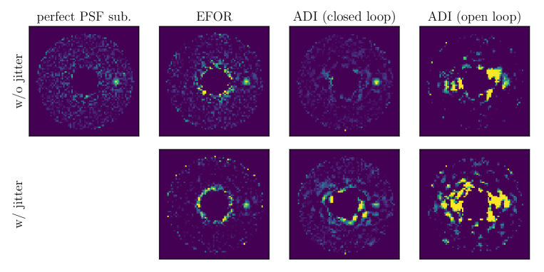
Figure 4: Incoherent intensity estimates of a planet at $6\>\lambda/D$, from left to right: Theoretical limit for a $30\>\mathrm{hr}$ long observation with a perfectly known PSF, highest contrast and no drifts or jitter; Electric Field Order Reduction (EFOR) for a closed-loop $30\>\mathrm{hr}$ long observation with one $26\>\mathrm{deg}$ telescope roll, only speckle (no DM) drift present and jitter either simulated (bottom) or not (top); Angular Differential Imaging (ADI) for a closed-loop $30\>\mathrm{hr}$ long observation with one $26\>\mathrm{deg}$ telescope roll; ADI for three open-loop $8\>\mathrm{hr}$ long observation, each starting from a “perfect” dark hole and including four $26\>\mathrm{deg}$ telescope rolls.

The authors have previously suggested that combining dark hole maintenance with EFOR could lead to smaller errors in post-processing[18]. Below, we re-assess this claim in the presence of jitter and high order DM drift (i.e., when each actuator drifts independently of all others). To this end, we use the data simulated in Sec. 2.4 while additionally introducing one $26\>\mathrm{deg}$ telescope roll. A planet with intensity of $5.0\>\frac{\mathrm{\mathrm{photon}}}{\mathrm{frame}}$ (across all wavelengths) was simulated at $6\>\lambda/D$.

Figure 4 (left) shows the baseline for post-processing evaluation – a simple PSF subtraction assuming that the speckle pattern remains fixed at its lowest average intensity and is perfectly known. In this “perfect” case, the PSF subtraction error is due to shot-noise alone and is therefore at its theoretical limit. In an open-loop scenario without DM drift and jitter, the Angular Differential Imaging (ADI) technique eliminated some, but not all of the speckle (Fig. 4 - right). In the closed-loop scenario ADI and EFOR preformed similarly, although the residual error of ADI is smoother (Fig. 4 middle).

To quantify the comparison we use the relative post-processing-error (PPE), based on the error of the estimated incoherent intensity in the region where the planet’s intensity is above its half-max,

$$\mbox{rel. PPE}=\frac{\mbox{avg. post-processing error }}{\mbox{avg. error of perfect PSF subtraction }}.$$ (36)

The relative PPE is always greater or equal to $1$ and, if the intensity of the speckles is uniformly distributed in time, is independent of the duration of the observation (in the limit of long observations). For the open-loop scenario we simulated three $8\>\mathrm{hr}$ fixed DM exposures (four rolls each) with dark hole “re-creation” between them ($80\%$ duty cycle), while the closed-loop simulations lasted $30$ hours and the contrast was maintained throughout. The potentially adverse effects of speckle drift induced by pointing maneuvers were not simulated.

Closing the loop always led to better relative PPEs, as illustrated in table 1 which is based on multiple realizations of each combination of a post-processing method and an observation scenario. Lowering the shot noise alone (see Sec. 2.4), reduces the errors by at least a factor of $2$. At the intermediate angular separation of $6\>\lambda/D$, ADI and EFOR performed similarly well, with the latter being able to identify and subtract the jitter modes when present. For lower angular separations, the PPE depends strongly on the jitter profile and roll sequences, although EFOR doesn’t suffer accuracy losses as much as ADI (this suggests that WFIRST has large sensitivity to jitter, although its quantitative analysis is beyond the scope of this paper). EFOR, however, breaks down in the presence of drift of statistically independent DM actuators since the resulting perturbations of the electric field are not low-order and have a larger amplitude than those of the speckles drift (arguably, this is only the case because DM drift is large compared to the low order Zernike drift).

	monochromatic	monochromatic	broadband
	w/o DM drift	w/o DM drift	w/ DM drift
	w/o jitter	w/ jitter	w/ jitter
open loop + ADI	3.0	4.5	12
closed loop +ADI	1.5	2.0	5
closed loop +EFOR	1.5	1.5	15

Table 1: Post-processing errors relative to PSF subtraction under perfect conditions (Eq. (36)) for various observation strategies (fixed DMs with periodic re-creation of the dark hole vs. closed-loop), instability sources (only drift in the first 21 Zernike modes, additional slowly varying residual jitter, additional high order DM actuators drift), detector types (IFS vs. broadband detectors) and post-processing algorithms (ADI vs. EFOR). Closed-loop strategy is always preferable to open-loop and ADI generally gets close to the theoretical detection limit. EFOR has a slight advantage since it is capable of identifying and subtracting “jitter modes” as long as the drift is not “high-order” as is the case in the pretense of DM drift.

4 Conclusions

In this work we reaffirmed the benefits of actively maintaining high contrast throughout coronagraphic observations in the presence of jitter, DM actuators drift and broadband detectors. Numerical simulations of WFIRST suggest that regardless of the observation parameters, closing the loop on the electric field in the dark hole reduces shot noise and therefore significantly increases the post-processing accuracy.

A continuous closed-loop observation strategy would allow detecting fainter planets compared to periodic re-creation of the dark hole by pointing the telescope at bright reference stars. Although not included in our analysis, slewing the telescope back and forth between target and reference stars might introduce thermal stresses which would negatively impact the stability of the wavefront. Active dark hole maintenance avoids such maneuvers and the lower duty cycle and destabilization risks associated with them.

In Sec. 2 we’ve shown that the averaged pointing jitter manifests itself as an incoherent source, while DM actuators drift is similar to high-order instabilities in other optical components (e.g., the primary mirror). Both effects decrease the contrast in the dark hole, but are implicitly tackled by existing batch and recursive electric field estimation algorithms. These approaches can be slightly modified to process broadband measurements by expressing them as an incoherent sum over several narrowband intensities.

Assuming that the jitter is well modelled by fast perturbations in just a few electric field modes (e.g., tip and tilt), they can be estimated together with the low-order speckle drift modes in post-processing via EFOR (accounting for possible telescope rolls, see Sec. 3). The jitter effects can then be subtracted in post-processing, resulting in a slightly better performance compared to ADI. However, EFOR is not applicable when the wavefront errors are dominated by high-order disturbances due to DM drift. In that case, the lowest post-processing error was achieved by a combination of dark hole maintenance and ADI.

Appendix A Broadband Pair-probing and EFC Conditioning

Below, we analyze the numerical conditioning of the pair-probing broadband electric field estimate in Eq. (26) and the corresponding EFC control, Eq. (27). Even though the latter is based on the former, there is a large discrepancy between their “relative errors” as depicted in Fig. 3(b). To see why this is the case, it is sufficient to consider a dark hole with a single ($n=1$) broadband detector ($m=1$ and $l>1$).

With $n=m=1$, eqs. (24) and (26) become

$$I^{DH}(\pm\delta\mathbf{u}_{j}) =\left(\mathbf{E}^{DH}\pm G^{U}\delta\mathbf{u}_{j}\right)^{T}\left(\mathbf{E}^{DH}\pm G^{U}\delta\mathbf{u}_{j}\right)+I^{DIJ}\in\mathbb{R},$$ (37)

$$4\begin{bmatrix}\left(G^{U}\delta\mathbf{u}_{1}\right)^{T}\\ \vdots\\ \left(G^{U}\delta\mathbf{u}_{s}\right)^{T}\end{bmatrix}\hat{\mathbf{E}}^{DH} \approx\begin{bmatrix}I^{DH}(+\delta\mathbf{u}_{1})-I^{DH}(-\delta\mathbf{u}_{1})\\ \vdots\\ I^{DH}(+\delta\mathbf{u}_{s})-I^{DH}(-\delta\mathbf{u}_{s})\end{bmatrix}\in\mathbb{R}^{s},$$ (38)

respectively. Denoting, $\delta C=\begin{bmatrix}\delta\mathbf{u}_{1}&\cdots&\delta\mathbf{u}_{s}\end{bmatrix}\in\mathbb{R}^{a\times s}$ with $a$ standing for the number of DM actuators, (38) can be rewritten as

$$4\left(G^{U}\delta C\right)^{T}\hat{\mathbf{E}}^{DH}\approx\mathbf{b},$$ (39)

with $G^{U}\in\mathbb{R}^{2l\times a}$, $\hat{\mathbf{E}}^{DH}\in\mathbb{R}^{2l}$ and $\mathbf{b}$ defined as the right-hand side of (38). The accuracy of $\hat{\mathbf{E}}^{DH}$ therefore depends on the condition number of $G^{U}\delta C$ which may be very large due to the ambiguity between speckles at different wavelengths. In particular, the rows of $G^{U}$which correspond to “nearby” wavelengths are “almost” collinear, a fact which was not accounted for in Sec. 2.5.

Let

$$G^{U} =U_{G}\Sigma_{G}V_{G}^{T},$$ (40)

$$\delta C =U_{C}\Sigma_{C}V_{C}^{T}$$ (41)

be the singular value decompositions of $G^{U}$ and $\delta C$ with $U_{G},\Sigma_{G}\in\mathbb{R}^{2l\times 2l}$, $V_{G}\in\mathbb{R}^{a\times 2l}$, $U_{C}\in\mathbb{R}^{a\times s}$ and $\Sigma_{C},V_{C}\in\mathbb{R}^{s\times s}$. The least squares solution of (39) is given by,

$$\hat{\mathbf{E}}^{DH}=\frac{1}{4}U_{G}\Sigma_{G}^{-1}\left(U_{C}^{T}V_{G}\right)^{+}\Sigma_{C}^{-1}V_{C}^{T}\mathbf{b}$$ (42)

where $\left(U_{C}^{T}V_{G}\right)^{+}$ is the pseudo-inverse of $U_{C}^{T}V_{G}$. Due to the above mentioned spectral ambiguity, the singular values of $G^{U}$ (on the main diagonal of $\Sigma_{G}$) may vary by several orders of magnitude. Hence, relatively small errors in $\mathbf{b}$, when amplified by $\Sigma_{G}^{-1}$, yield large errors in the estimate, $\hat{\mathbf{E}}^{DH}$, as illustrated in Fig. 3(b).

However, to compute the control, $\Delta\mathbf{u}^{DH}$, the estimate is multiplied by the EFC gain in Eq. (27). This gain is given by

$$K_{EFC}=\left(\left(G^{U}\right)^{T}G^{U}+\mu I\right)^{-1}\left(G^{U}\right)^{T},$$ (43)

where $\mu>0$ is a regularization constant which makes $\left(G^{U}\right)^{T}G^{U}+\mu I$ well conditioned. Together with eqs. (40) and (42), the control becomes

$$\Delta\mathbf{u}^{DH}=-K_{EFC}\hat{\mathbf{E}}^{DH}=-\frac{1}{4}\left(V_{G}\Sigma_{G}^{2}V_{G}^{T}+\mu I\right)^{-1}V_{G}\left(U_{C}^{T}V_{G}\right)^{+}\Sigma_{C}^{-1}V_{C}^{T}\mathbf{b},$$ (44)

and does not contain the ill-conditioned $\Sigma_{G}^{-1}$. Indeed, $\Delta\mathbf{u}^{DH}$ is not severely affected by measurement errors and non-linearities: in the numerical results of Sec. 2.5, each additional pixel increases the relative error in $\Delta\mathbf{u}^{DH}$ by about $3\%$ (and since there are $n=2608$ pixels, the total relative error is about $\sqrt{2608}\cdot 0.03\approx 1.5$, as seen in Fig. 3(b)).

References

- [1] C. C. Stark et al., “Exoearth yield landscape for future direct imaging space telescopes,” Journal of Astronomical Telescopes, Instruments, and Systems 5(2), 1 – 20 (2019).
- [2] B.-J. Seo et al., “Testbed demonstration of high-contrast coronagraph imaging in search for earth-like exoplanets,” in Techniques and Instrumentation for Detection of Exoplanets IX, S. B. Shaklan, Ed., Proc.SPIE 11117, 599 – 609, International Society for Optics and Photonics, SPIE (2019).
- [3] E. S. Douglas et al., “Wfirst coronagraph technology requirements: status update and systems engineering approach,” in Modeling, Systems Engineering, and Project Management for Astronomy VIII, 10705, 1070526, International Society for Optics and Photonics (2018).
- [4] R. Demers, “Review and update of WFIRST coronagraph instrument design and technology (conference presentation),” in Space Telescopes and Instrumentation 2018: Optical, Infrared, and Millimeter Wave, Proc.SPIE 10698 (2018).
- [5] B. Nemati, J. E. Krist, and B. Mennesson, “Sensitivity of the WFIRST coronagraph performance to key instrument parameters,” in Techniques and Instrumentation for Detection of Exoplanets VIII, Proc.SPIE 10400, 1040007, International Society for Optics and Photonics (2017).
- [6] S. B. Shaklan et al., “Stability error budget for an aggressive coronagraph on a 3.8 m telescope,” in Techniques and Instrumentation for Detection of Exoplanets V, Proc.SPIE 8151, 815109, International Society for Optics and Photonics (2011).
- [7] H. Zhou et al., “High accuracy coronagraph flight WFC model for WFIRST-CGI raw contrast sensitivity analysis,” in Space Telescopes and Instrumentation 2018: Optical, Infrared, and Millimeter Wave, M. Lystrup, H. A. MacEwen, G. G. Fazio, et al., Eds., 10698, 811 – 824, International Society for Optics and Photonics, SPIE (2018).
- [8] G. Ruane et al., “Performance and sensitivity of vortex coronagraphs on segmented space telescopes,” in Techniques and Instrumentation for Detection of Exoplanets VIII, S. Shaklan, Ed., Proc.SPIE 10400, 140 – 155, International Society for Optics and Photonics, SPIE (2017).
- [9] B. Mennesson et al., “The habitable exoplanet (HabEx) imaging mission: preliminary science drivers and technical requirements,” in Space Telescopes and Instrumentation 2016: Optical, Infrared, and Millimeter Wave, H. A. MacEwen, G. G. Fazio, M. Lystrup, et al., Eds., Proc.SPIE 9904, 212 – 221, International Society for Optics and Photonics, SPIE (2016).
- [10] M. R. Bolcar et al., “The large uv/optical/infrared surveyor (LUVOIR): Decadal mission concept design update,” in UV/Optical/IR Space Telescopes and Instruments: Innovative Technologies and Concepts VIII, H. A. MacEwen and J. B. Breckinridge, Eds., Proc.SPIE 10398, 79 – 102, International Society for Optics and Photonics, SPIE (2017).
- [11] V. P. Bailey et al., “Lessons for wfirst cgi from ground-based high-contrast systems,” in Space Telescopes and Instrumentation 2018: Optical, Infrared, and Millimeter Wave, 10698, 106986P, International Society for Optics and Photonics (2018).
- [12] A. Give’on, B. D. Kern, and S. B. Shaklan, “Pair-wise, deformable mirror, image plane-based diversity electric field estimation for high contrast coronagraphy,” in Techniques and Instrumentation for Detection of Exoplanets V, Proc.SPIE 8151, 815110, International Society for Optics and Photonics (2011).
- [13] A. Give’on et al., “Electric field conjugation-a broadband wavefront correction algorithm for high-contrast imaging systems,” in Bulletin of the American Astronomical Society, 39, 975 (2007).
- [14] J. Krist et al., “WFIRST coronagraph flight performance modeling,” in Space Telescopes and Instrumentation 2018: Optical, Infrared, and Millimeter Wave, M. Lystrup, H. A. MacEwen, G. G. Fazio, et al., Eds., Proc.SPIE 10698, 788 – 810, International Society for Optics and Photonics, SPIE (2018).
- [15] L. Pogorelyuk and N. J. Kasdin, “Dark hole maintenance and a posteriori intensity estimation in the presence of speckle drift in a high-contrast space coronagraph,” The Astrophysical Journal 873, 95 (2019).
- [16] F. Shi et al., “WFIRST low order wavefront sensing and control (LOWFS/C) performance on line-of-sight disturbances from multiple reaction wheels,” in Techniques and Instrumentation for Detection of Exoplanets IX, S. B. Shaklan, Ed., Proc.SPIE 11117, 170 – 178, International Society for Optics and Photonics, SPIE (2019).
- [17] C. M. Prada, E. Serabyn, and F. Shi, “High-contrast imaging stability using MEMS deformable mirror,” in Techniques and Instrumentation for Detection of Exoplanets IX, S. B. Shaklan, Ed., Proc.SPIE 11117, 112 – 118, International Society for Optics and Photonics, SPIE (2019).
- [18] L. Pogorelyuk, N. J. Kasdin, and C. W. Rowley, “Reduced order estimation of the speckle electric field history for space-based coronagraphs,” The Astrophysical Journal 881, 126 (2019).
- [19] P. J. Lowrance et al., “A coronagraphic search for substellar companions to young stars,” in NICMOS and the VLT: A New Era of High Resolution Near Infrared Imaging and Spectroscopy, W. Freudling and R. Hook, Eds., European Southern Observatory Conference and Workshop Proceedings 55, 96, European Southern Observatory (1998).
- [20] C. Marois et al., “Angular differential imaging: A powerful high-contrast imaging technique,” The Astrophysical Journal 641, 556–564 (2006).
- [21] N. Jovanovic et al., “Review of high-contrast imaging systems for current and future ground-based and space-based telescopes: Part II. common path wavefront sensing/control and coherent differential imaging,” in Adaptive Optics Systems VI, Proc.SPIE 10703 (2018).
- [22] A. E. Riggs, N. J. Kasdin, and T. D. Groff, “Optimal wavefront estimation of incoherent sources,” in Space Telescopes and Instrumentation 2014: Optical, Infrared, and Millimeter Wave, Proc.SPIE 9143, 914324, International Society for Optics and Photonics (2014).
- [23] L. Pogorelyuk, C. W. Rowley, and N. J. Kasdin, “An efficient approximation of the kalman filter for multiple systems coupled via low-dimensional stochastic input,” arXiv preprint arXiv:1911.10443 (2019).
- [24] A. E. Riggs et al., “Fast linearized coronagraph optimizer (FALCO) I: a software toolbox for rapid coronagraphic design and wavefront correction,” in Space Telescopes and Instrumentation 2018: Optical, Infrared, and Millimeter Wave, H. A. MacEwen, M. Lystrup, G. G. Fazio, et al., Eds., Proc.SPIE 10698, SPIE (2018).
- [25] D. Mawet, B. Mennesson, E. Serabyn, et al., “A dim candidate companion to Epsilon Cephei,” The Astrophysical Journal Letters 738(1), L12 (2011).
- [26] R. Soummer, L. Pueyo, and J. Larkin, “Detection and characterization of exoplanets and disks using projections on Karhunen-Loève eigenimages,” The Astrophysical Journal Letters 755, L28 (2012).
- [27] A. Amara and S. P. Quanz, “PYNPOINT: An image processing package for finding exoplanets,” Monthly Notices of the Royal Astronomical Society 427, 948–955 (2012).
- [28] B. Ren et al., “Non-negative matrix factorization: Robust extraction of extended structures,” The Astrophysical Journal 852, 104 (2018).
- [29] L. Pogorelyuk and N. J. Kasdin, “Maintaining a dark hole in a high contrast coronagraph and the effects of speckles drift on contrast and post processing factor,” in Techniques and Instrumentation for Detection of Exoplanets IX, S. B. Shaklan, Ed., Proc.SPIE 11117, 397 – 403, International Society for Optics and Photonics, SPIE (2019).