Adversarial Examples Detection and Analysis with Layer-wise Autoencoders

Abstract

We present a mechanism for detecting adversarial examples based on data representations taken from the hidden layers of the target network. For this purpose, we train individual autoencoders at intermediate layers of the target network. This allows us to describe the manifold of true data and, in consequence, decide whether a given example has the same characteristics as true data. It also gives us insight into the behavior of adversarial examples and their flow through the layers of a deep neural network. Experimental results show that our method outperforms the state of the art in supervised and unsupervised settings.

1 Introduction

Deep neural networks have shown impressive performance on various machine learning tasks including object detection (Zhao et al., 2019), speech recognition (Amodei et al., 2016), image classification (He et al., 2016), etc. While these models are usually robust to random noise, their performance can dramatically deteriorate under adversarial perturbations, i.e., small changes of the input which are imperceptible to humans, but mislead the model to output wrong predictions (Szegedy et al., 2013; Goodfellow et al., 2014). This phenomenon can disqualify a model from applications such as autonomous cars or banking systems, where security is a priority (Sitawarin et al., 2018; Grosse et al., 2017b).

Several methods have been proposed to defend the deep learning models against adversarial attacks. One approach relies on adding adversarial examples to the training stage, which makes the model robust to many (but not all) adversarial attacks (Madry et al., 2017). To give formal guarantees that no adversarial perturbation within a given range fools a neural network, more computationally demanding provable defenses are used. These methods employ either integer programming approaches (Lomuscio & Maganti, 2017; Xiao et al., 2018), Satisfiability Modulo Theories (SMT) solvers (Carlini et al., 2017; Ehlers, 2017) or computing an approximation to the adversarial polytope (Zhang et al., 2018; Morawiecki et al., 2019). All of the aforementioned approaches involve special training procedures and, in consequence, they cannot be used when the target neural network is fixed (we are not allowed to modify or retrain it from scratch).

The other line of research, which is considered in this paper, relies on introducing auxiliary mechanisms to detect whether the input can be seen as an adversarial example without modifying the target model. Most methods employ a supervised approach and train a classifier to discriminate normal samples from adversarial examples (Hendrycks & Gimpel, 2016). In (Lee et al., 2018), the authors propose to estimate the class-conditional Gaussian distribution in each layer and use the Mahalanobis distance to discriminate adversarial examples. A different approach is to consider the unsupervised detection of abnormal samples. In (Xu et al., 2017), adversarial examples are detected by comparing the model’s predictions on a given input with its predictions on a squeezed version of the input. The authors of (Yang et al., 2019) propose a detection mechanism based on the observation that the feature attribution map of an adversarial example near the boundary always differs from that of the corresponding original example. In (Roth et al., 2019), the authors introduce a statistical test based on the change of feature representations and log-odds under noise. The authors of (Samangouei et al., 2018) use GANs to model the distribution of unperturbed images and, in consequence, find a close output to a given image which does not contain the adversarial changes. An interesting analysis in (Papernot & McDaniel, 2018), which partially inspired the presented paper, shows how the representation of an adversarial example changes through neural network layers.

The primary goal of this paper is to characterize and analyze the behavior of the adversarial examples, see Section 2 for the formulation of our hypotheses and Section 3 for experimental evidence. Our first observation shows that as we increase the perturbation, the movement of adversarial examples from the true data manifold is stronger than their movement within that manifold. The second observation is that the deviation of adversarial examples from the normal data manifold can be observed in the hidden layers of the target network and the deepest layers are the most discriminative. Our analysis extends the recent works concerning adversarial attacks (Lee et al., 2018; Papernot & McDaniel, 2018; Pidhorskyi et al., 2018).

Figure 1: The scheme of the proposed detection method. We train individual autoencoders on hidden representations of the pre-trained target network to describe the manifold of true data. Features from the autoencoders are used by an external classifier to detect the adversarial examples.

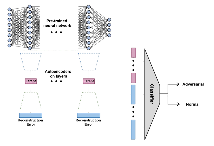
Our second contribution is a method for detecting adversarial examples based on data representation taken from the hidden layers of the target network, see Figure 1. For this purpose, we train individual generative autoencoders at hidden layers of the target network. This allows us to describe the original data manifold and helps to decide whether a given example has the same characteristic as the actual data. We stress that our solution does not require retraining of the target network, so it can be applied to existing models without modifying them.

Experiments performed on the ResNet and DenseNet architectures show that the implementation of our method gives the highest detection rate among recent detection methods, see Table 1. Moreover, our analysis sheds a new light on the understanding of the behavior of adversarial examples.

2 Detection and Analysis of Adversarial Examples

Before we describe the detection method, let us first discuss our observations regarding the behavior of the adversarial examples in deep neural networks. We start with the basics of adversarial examples and generative models. Next, we formalize our research hypotheses, which describe the behavior of adversarial examples in neural network layers. This analysis naturally leads us to the detection algorithm.

2.1 Preliminaries

Neural network. We consider a neural network $F:\mathbb{R}^{D}\to\mathbb{R}^{K}$, which maps the input data $X\subset\mathbb{R}^{D}$ to the logit outputs for the $K$-class classification problem. The network is composed of $L$ layers $h_{l}$:

$$z_{l}=h_{l}(z_{l-1}),\text{ for }l=1,\ldots,L.$$

A final classification is obtained by applying the softmax function $S$ to the logits $z_{L}$.

Adversarial attack. Typical classification networks tend to have strong predictions on unseen data. For example, if a network is trained on the classes "1-9" of the MNIST data set, it will also provide strong predictions for elements of class "0". In other words, a basic classification network cannot reliably estimate the uncertainty of the predictions, which, in particular, makes it vulnerable to adversarial attacks.

In adversarial attacks, the attacker adds a small perturbation $\delta$ to the input $x$, such that a neural network gives wrong prediction, i.e.,

$$\arg\max_{i}S(F(x+\delta))_{i}\neq y_{true},$$

where $y_{true}$ denotes the true class label of $x$. The perturbed input $x+\delta$, which causes the network to misclassify $x$, is called an adversarial example. For most adversarial attacks we assume that the perturbation magnitude $\delta$ cannot be bigger than a fixed value $\varepsilon$ measured by the distance metric $d$.

Autoencoders. According to the manifold hypothesis, high-dimensional data tend to lie in a low-dimensional manifold (Fefferman et al., 2013). One approach for describing a data manifold is to use the autoencoder model. The classical autoencoder (AE) consists of the encoder $\mathcal{E}$ and the decoder $\mathcal{D}$. The encoder transports the input data to a generally lower-dimensional latent space $\mathcal{E}:\mathbb{R}^{d}\to Z=\mathbb{R}^{n}$, whereas the decoder transforms the latent $Z$ back to the original space $\mathcal{D}:Z\to\mathbb{R}^{d}$. We search for $\mathcal{E}$ and $\mathcal{D}$ such that the reconstruction error

$$Error(X;\mathcal{E},\mathcal{D})=\sum_{x\in X}\|x-\mathcal{D}(\mathcal{E}(x))\|^{2}$$

is minimized, where $X\subset\mathbb{R}^{d}$ denotes the training data. Intuitively, the reconstruction error describes a distance of a given sample from the manifold.

If we want to additionally model a probability distribution of data on that manifold, we can define a prior distribution $f$ (typically Gaussian) in the latent space and optimize the distance of $\mathcal{E}(x)$ from the prior, which is the basic idea of the autoencoder-based generative models (Tabor et al., 2018). In the case of the Variational AutoEncoder (VAE) (Kingma & Welling, 2014), the discrepancy between $\mathcal{E}(x)$ and $f$ is measured via the Kullback-Leibler divergence. In the Wasserstein autoencoder (WAE) (Tolstikhin et al., 2018), we use the Wasserstein distance (implemented either as the MMD or GAN loss).

2.2 Adversarial examples dynamics

The main idea pursued in this paper is that adversarial examples have a different distribution from normal data (Grosse et al., 2017a). To quantify this discrepancy, we formulate two hypotheses. The first one states that the increase of the perturbation magnitude pushes adversarial examples further from the manifold of normal data. The second one states that the distribution disagreement cannot be easily detected in the original data representation (inputs), but can be observed in the hidden layers of the target network. The hypotheses verification is the subject of Section 3.

Influence of perturbation magnitude. We assume that $M$ is the manifold of normal data $X\subset\mathbb{R}^{D}$. Let us consider the $\varepsilon$-bounded attack, where the attacker is allowed to perturb the input data point $x$ by a maximal value $\varepsilon$. To illustrate the dependence of an adversarial example on the maximal perturbation $\varepsilon$, we consider the curve:

$$\gamma:\varepsilon\to x_{\varepsilon},$$

which for a given $\varepsilon$ and a fixed $x\in X$ returns an adversarial example $x_{\varepsilon}=x+\delta$, where $\delta\in[\varepsilon,\varepsilon]^{D}$. In other words, we look at the trajectory of the adversarial example with the increasing magnitude of the perturbation.

From this point of view, we can decompose the curve $\gamma$ into the component from data manifold $M$ and its orthogonal complement as:

$$\gamma=\gamma_{M}+\gamma_{\perp M},$$

where

$$\gamma_{M}(\varepsilon)\in M,\gamma_{\perp M}(\varepsilon)-\gamma_{M}(\varepsilon)\perp T_{\gamma_{M}(\varepsilon)}M.$$

and $T_{\gamma_{M}(\varepsilon)}$ is a tangent space to $M$ at the point $\gamma(\varepsilon)$. Generally, we choose $\gamma_{M}(\varepsilon)$ to be the nearest point in $M$ from $\gamma(\varepsilon)$.

The main question is: which of these two components has a stronger influence on the construction of adversarial examples?

Adversarial dynamics hypothesis: The movement perpendicular to the manifold $M$ of true data is dominant for the construction of adversarial examples, i.e., the deviation of $\gamma_{\perp M}(\varepsilon)$ is higher than the deviation of $\gamma_{M}(\varepsilon)$, with the increasing value of the maximal perturbation $\varepsilon$.

In the context of generative AEs:

• The movement along $\gamma_{\perp M}$ is quantified by the reconstruction error. This coincides with a discrepancy between a given sample and the data manifold.

• The movement within $\gamma_{M}$ is quantified by the norm in the latent space. It shows whether a data point is generated from the data distribution on that manifold.

Reconstruction error propagation through layers. According to the previous hypothesis, adversarial examples move far apart from data manifold as the perturbation magnitude increases. However, since the difference between clean and adversarial examples is very small, it is usually difficult to detect adversarial attacks using their initial representation (inputs to the network). To overcome this difficulty, we study the hidden layers of the network. Since each layer gives a different representation of the same data, we can now ask: which layer has the highest discriminative power in the context of adversarial examples?

Observe that the network is, in fact, a composition of nonlinear maps

$$F=h_{L}\circ\ldots\circ h_{1}.$$

Since, in practice, each of these maps has the Lipschitz constant $\mathrm{lip}(h_{l})$ greater than $1$, we can argue that a small movement in the input space may result in a very large representation distance in the last layers. Moreover, in high-dimensional spaces we usually have

$$\mathrm{lip}(F)\approx\mathrm{lip}(h_{1})\cdot\ldots\cdot\mathrm{lip}(h_{L}).$$

Consequently, with a very small change in the input, we expect high divergence from the manifold of normal data, which is the main point of our second hypothesis:

Layers dynamics hypothesis: The divergence of adversarial examples from the manifold (and corresponding distribution) of normal data is more evident in the consecutive hidden layers than in the initial representation.

Exploration of this hypothesis is also motivated by other works where information is gathered and combined from the hidden layers. In (Papernot & McDaniel, 2018), an adversarial example is compared to the closest neighbor from the training set on a layer-by-layer basis; in (Lee et al., 2018), the Mahalanobis distance is calculated between the adversarial example and the training set, also across the layers.

Figure 2: Impact of adversarial perturbations on the position of an example in 2D space (reconstruction error in the x-axis and latent $L_{2}$ norm in the y-axis). The starting point is a single normal example without any perturbations (visualized as a light yellow dot). Then, we linearly increase the perturbation until it reaches the value of $2\epsilon$ (dark red). The $\epsilon$ values for a given network architecture/dataset are the same as in (Lee et al., 2018). As a point of reference, we provide the kernel density estimation (green) of normal examples from the test set. Each column of sub-figures refers to a different attack and each row of sub-figures refers to a different layer. The experiments shown here are for the Densenet architecture and the CIFAR-100 dataset. The crucial observation is that adversarial examples significantly move away from the data manifold as the perturbation magnitude increases (movement in x-axis).

2.3 Detection Mechanism

Based on the aforementioned hypotheses, we formulate a mechanism for detecting abnormal samples, depicted in Figure 1.

To describe the manifold of normal data $X$, we train individual generative autoencoders at consecutive layers of the network $F$. To reduce training and testing time, we use only selected layers of the network. We emphasize that only the normal data is used for the autoencoder training and the target network weights remain unmodified.

As explained, the reconstruction error and the latent norm can be seen as two factors that measure the discrepancy from data manifold and divergence from the corresponding distribution. In consequence, the classification system, which is responsible for detecting abnormal samples, is trained on these features. More precisely, we collect these two features from all AEs and pass them to a given classifier. In the experiments, we also investigate the situation when AEs are represented by the full latent vectors instead of the reconstruction error and the latent norm. This alternative representation can be more meaningful, but, one the other hand, the classification model is more time consuming to train and test on that high-dimensional space.

Our method can be applied to two real-life scenarios. In the first one, we assume that our system is targeted for a specific attack type. In this case, we train a (fully supervised) classifier on normal and adversarial examples. In a more realistic scenario, where the type of an adversarial attack is unknown, we cannot train the final classifier in the supervised way as we lack the second (adversarial) class examples. In this situation, we build a one-class classifier, which is trained only on normal data. In the test stage, we verify whether a sample belongs to data or not.

3 Analysis of Adversarial Examples Dynamics

In this section, we experimentally verify the hypotheses formulated in Section 2. For this purpose, we use two modern CNN architectures: ResNet and DenseNet for three classification tasks: CIFAR-10, CIFAR-100, and SVHN. We consider five different attacks: FGSM, BIM, DeepFool, CW ($L_{2}$) and PGD ($L_{\inf}$, 100 iterations). To implement our detection mechanism, we train WAE-MMD autoencoders on the representations taken from selected hidden layers using training data. More details on training parameters and the experiment setup are given in Section 4, where we present the results for the detection problem.

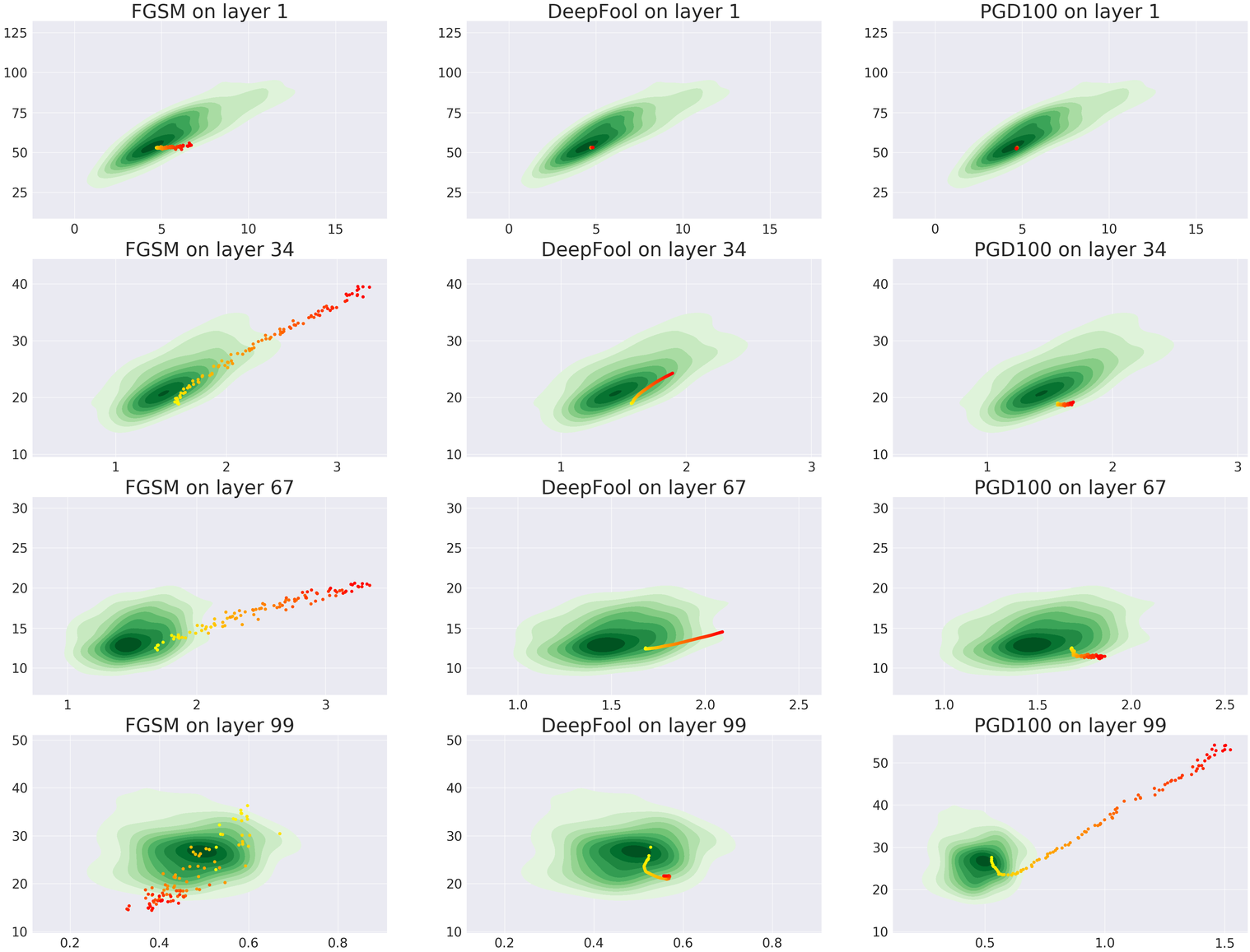
Deviation from data manifold (Hypothesis 1). In the first experiment, we investigate the influence of the perturbation magnitude on the location of adversarial examples in the normal data distribution. For this purpose, we generate adversarial examples with increasing values of $\varepsilon$ for three types of attacks. We visualize the experiment in 2D space, where the x-axis is the reconstruction error of the WAE autoencoder and the y-axis is the $L_{2}$ norm in the latent space. The experiment is performed on the CIFAR-10 dataset and the ResNet architecture. We provide figures for all other dataset-architecture combinations in Supplementary Material, Section B.

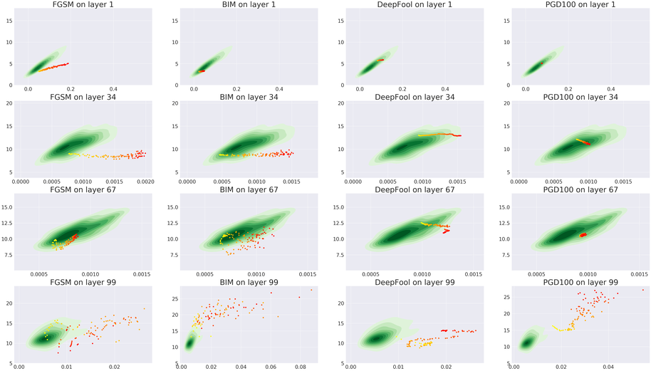
It is evident from Figure 2 that the curve $\gamma(\varepsilon)$ gradually moves away from the distribution of normal data. The movement in the direction perpendicular to the data manifold (x-axis) is stronger than within the manifold (y-axis). This discrepancy is most evident in layers 34 and 99 (second and fourth rows). It partially confirms that the movement in the direction perpendicular to data manifold is essential.

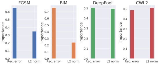
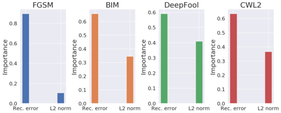
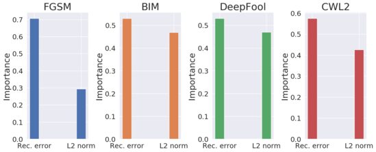
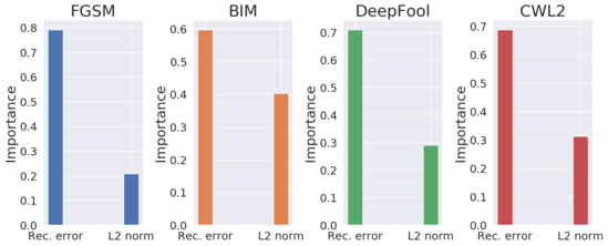
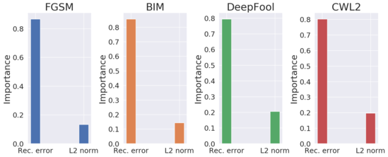
To support our analysis in a more quantitative way, we assess the feature importance in the detection context. For this purpose, we consider supervised and unsupervised settings. In the first case, we train a random forest classifier on the composition of the reconstruction error and the latent norm from each WAE. As a result, we obtain the importance of each feature, which are aggregated over the layers to get the summarized importance of the reconstruction error and the latent norm. In the unsupervised case, we report the performance of one-class classifier (implemented as the Isolation Forest) trained on either the reconstruction error only, the latent norm only, or on both features. The results presented in Supplementary Material, Section D show that the reconstruction error is significantly more important than the latent norm for the detection of abnormal samples. We also conduct a similar ablation study for the supervised classifier, where the detector is trained in a few scenarios, each with a different set of features (see Supplementary Material, Section E). These findings confirm our hypothesis that adversarial examples deviate from the data manifold more than from the distribution on that manifold.

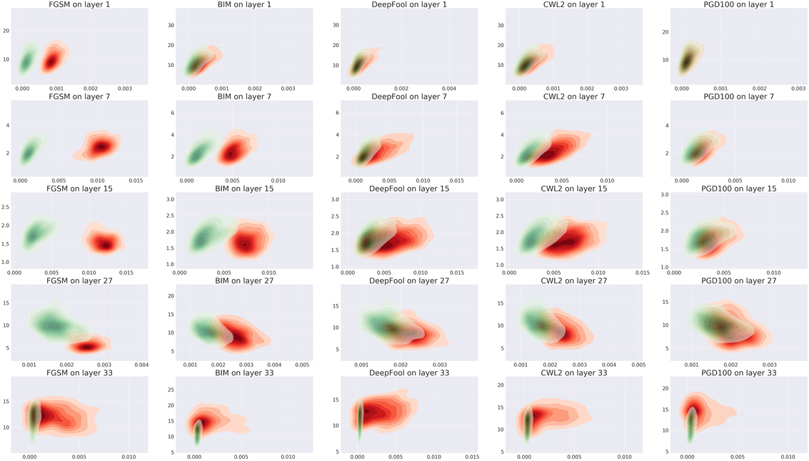
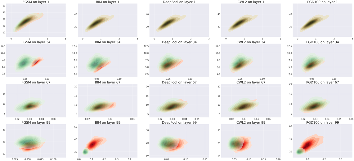
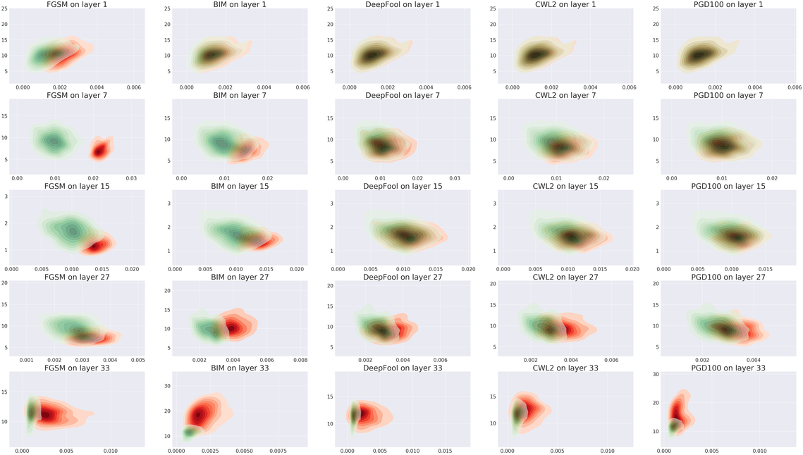
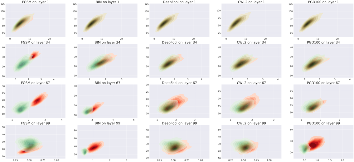
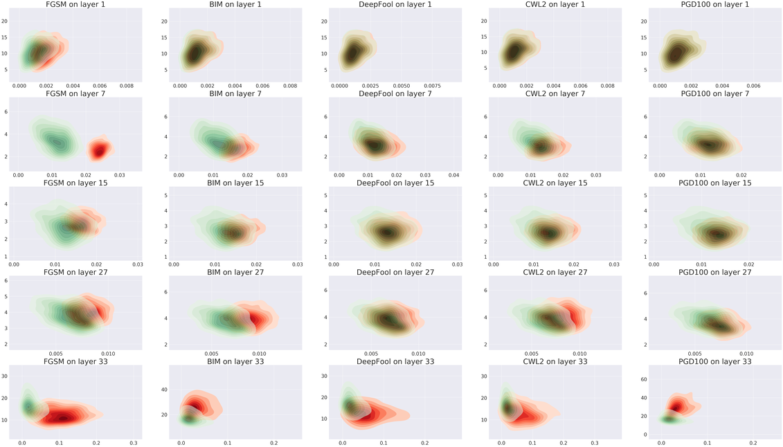
Distributions in consecutive hidden layers (Hypothesis 2). We examine which layer of the target network is the most discriminative for detecting adversarial examples. For this purpose, we plot the distribution of normal and adversarial samples in 2D space given by the reconstruction error and the latent norm for WAE in consecutive layers of the target network.

Figure 3: The normal (green) and adversarial (red) examples visualized by the kernel density estimation in 2D space. In each sub-figure, the x-axis is the reconstruction error, the y-axis is the norm in the latent space. Each column of sub-figures refers to a different attack. These figures are generated for the SVHN dataset, DenseNet architecture. The adversarial examples are followed through 4 autoencoders, hence 4 rows of sub-figures. In most cases, the discrepancy between these distributions is most evident in the last layers. However, for simple attacks such as FGSM, adversarial examples can also be easily detected in earlier layers.

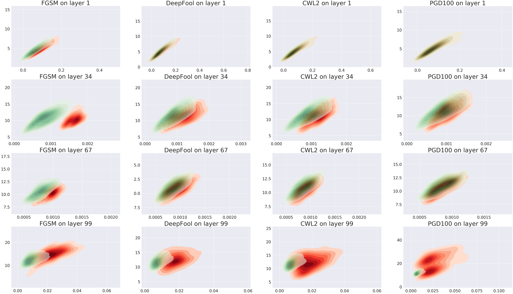
Figure 3 demonstrates that in nearly every setting, we can identify a layer where the distribution of normal and adversarial examples diverge. At first glance, deeper layers have the highest discriminative power. More careful analysis suggests, however, that for simple attacks, such as FGSM, initial layers also deliver substantial information for detection of abnormal samples (second row). For stronger attacks (DeepFool and CW) this discrepancy is not evident in the initial layers and the behavior in the last layers has to be investigated. For figures from other dataset-architecture combinations, we refer the reader to Supplementary Material, Section A.

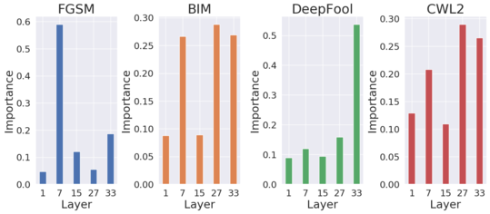
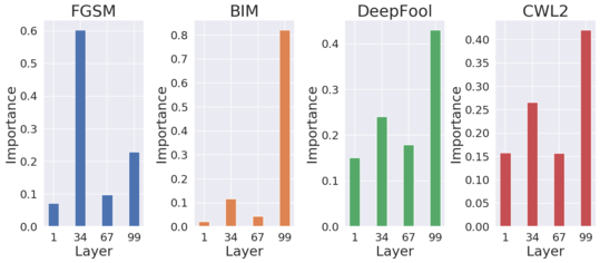
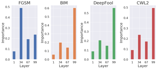
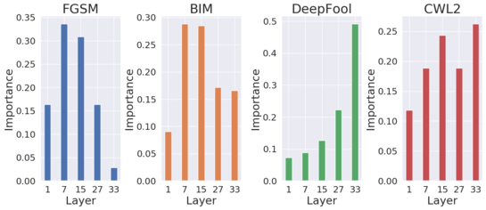
To summarize this analysis in a quantitative way, we again analyze the importance of features using a random forest classifier. This time, we aggregate the importance of the reconstruction error and the latent norm for a given layer to get the total layer importance. Visualization of the layer importance (see Supplementary Material, Section C) confirms that for the FGSM attack, the most discriminative layer is the one after the first block, whereas the last two blocks are more important for other types of attacks. For simpler attacks, such as the FGSM, the adversarial examples quickly escape from the normal data manifold, hence earlier layers become important. More sophisticated attacks, such as DeepFool, CW and PGD, keep the adversarial example representations inside the normal data manifold for multiple layers, hence the final layer is the most discriminative for those attacks.

4 Experiments

Model	Dataset	Method	Supervised setting					Unsupervised setting
			FGSM	BIM	DeepFool	CW	PGD	FGSM	BIM	DeepFool	CW	PGD
DenseNet	CIFAR-10	Odds-testing	-	-	-	-	-	45.23	69.01	58.30	61.29	97.93
		Mahalanobis	99.94	99.78	83.41	87.31	97.79	-	-	-	-	-
		AE-layers (ours)	100.00	99.99	91.36	97.75	99.61	78.38	97.51	65.31	68.15	94.20
	CIFAR-100	Odds-testing	-	-	-	-	-	43.22	65.22	49.53	47.64	96.91
		Mahalanobis	99.86	99.17	77.57	87.05	79.24	-	-	-	-	-
		AE-layers (ours)	100.00	99.88	88.17	96.40	96.63	97.95	95.68	61.86	62.28	87.19
	SVHN	Odds-testing	-	-	-	-	-	56.14	71.11	67.81	70.71	99.25
		Mahalanobis	99.85	99.28	95.10	97.03	98.41	-	-	-	-	-
		AE-layers (ours)	99.98	99.75	97.26	97.80	99.43	96.50	94.07	83.80	84.81	93.70
ResNet	CIFAR-10	Odds-testing	-	-	-	-	-	46.32	59.85	75.58	57.58	96.18
		Mahalanobis	99.94	99.57	91.57	95.84	89.81	-	-	-	-	-
		AE-layers (ours)	99.98	99.61	86.41	95.01	97.39	97.24	94.93	78.19	74.29	77.25
	CIFAR-100	Odds-testing	-	-	-	-	-	38.26	43.52	61.13	44.74	93.73
		Mahalanobis	99.77	96.90	85.26	91.77	91.08	-	-	-	-	-
		AE-layers (ours)	100.00	99.52	77.98	96.41	98.12	95.59	80.23	71.06	73.02	70.98
	SVHN	Odds-testing	-	-	-	-	-	65.09	70.31	77.05	72.12	99.08
		Mahalanobis	99.62	97.15	95.73	92.15	92.24	-	-	-	-	-
		AE-layers (ours)	99.81	99.10	95.45	97.31	97.41	98.90	95.49	89.36	90.02	83.62

Table 1: Comparison of AUROC (%) scores. For the supervised setting, we use SVM as the final classifier and the entire latent vectors as its input features. For the unsupervised setting, we use Isolation Forest as the one-class classifier with the reconstruction errors and the latent norms as input features.

We test our method against FGSM (Goodfellow et al., 2014), BIM (Kurakin et al., 2016), DeepFool (Moosavi-Dezfooli et al., 2016), CW (Carlini & Wagner, 2017) and PGD (Madry et al., 2017) adversarial attacks on CIFAR-10 (Krizhevsky et al., a), CIFAR-100 (Krizhevsky et al., b) and SVHN (Netzer et al., 2011) datasets for ResNet-34 (He et al., 2016) and DenseNet-BC (L = 100, k = 12) (Huang et al., 2017) models. To reduce the computational time, we train WAE-MMD autoencoders on the selected layers of the target network. Specifically, we select the layers ending each block group in those architectures – the same approach as in (Lee et al., 2018). For simplicity, we use the same hyperparameters for each autoencoder and if the representation size allows, the same architecture, even between datasets and models.

For the sake of a fair comparison, we use the test set creation procedure from (Lee et al., 2018). In that setting, a noisy and an adversarial sample is created for each test set sample. The final test set consists of correctly classified clean and noisy examples (class 1) and incorrectly classified adversarial examples (class 2). In the supervised detection of adversarial examples, the final classifier is trained on 10% of that test set and is evaluated on the remaining 90%. For our methods (AE-layers), we use SVM as the final detection classifier with its hyperparameters being selected by 5-fold cross-validated grid search trained on the full AE latent vectors. In the unsupervised setting, we use the Isolation Forest one-class classifier, which is trained only on the training data without seeing any adversarial or noisy examples. To reduce the data dimension, we use a representation consisting of the reconstruction error and the $L_{2}$ norm taken from each autoencoder.

Table 1 shows the results for our method compared to two state-of-the-art studies: Mahalanobis (Lee et al., 2018) (for the supervised case) and Odds-testing (Roth et al., 2019) (for the unsupervised case). In the supervised case, our method provides better results for almost all investigated cases. In the unsupervised case, our method is inferior only on the PGD-100 attack. While Odds-testing performs particularly well on that attack, it fails on other types of attacks, which were not tested in the original paper. We also highlight that our solution is more efficient than Odds-testing approach. Odds-testing requires multiple forward passes of the target network (256 in the original version) for each example to be tested, which is computationally expensive. In comparison, the inference in our method is cheap as the forward pass of several shallow (3-layer) encoders is faster than one forward pass of the target network.

In (Lee et al., 2018) authors do not provide a fully unsupervised solution and they consider only a partially supervised scenario. In Supplementary Material, Section F we report the results for such a setting.

To compare the discriminative power of AE representations, we also run the supervised variant of our method trained on the reconstruction error and the latent norm. With the reduced representation the results are nearly the same. Precisely, the results drop only $0.01$ in terms of the mean AUROC score compared to the the analogical variant trained on full latent space of AE. (See Supplementary Material, Section E for detailed results.) This analysis gives a strong argument that the reconstruction error and the latent norm provides sufficient description of data manifold to detect adversarial examples. Moreover, it greatly accelerates training making our approach easy to use in various applications.

5 Conclusion

We presented a novel method for adversarial example detection that achieves state-of-the-art performance. It is based on two hypotheses that essentially outline the design of our method by pointing out that adversarial examples diverge from normal samples data manifold on different layers of the original network. We perform a thorough experimental analysis to confirm these hypotheses and then evaluate and compare our detector with two other methods in both supervised and unsupervised settings. The inference in our solution is fast and unlike Odds-testing it does not require multiple forward passes.

Broader Impact

A successful detection of adversarial examples is essential to establish trust and reliability of deep neural networks. It is hard to imagine a trustworthy self-driving car with a deep learning system, which can be easily fooled by an adversarial example. Or a classifier detecting cancer and giving a wrong prediction due to tiny perturbations which look like meaningless artifacts. Providing an additional mechanism, which detects adversarial examples helps to make the neural nets more applicable to real world problems. On the other hand, one must be very careful about guarantees given by such defenses. Typically, we aim at concrete attacks and scenarios, so more general claims may not be valid.

Appendix A Distribution of Normal and Adversarial Examples Representation

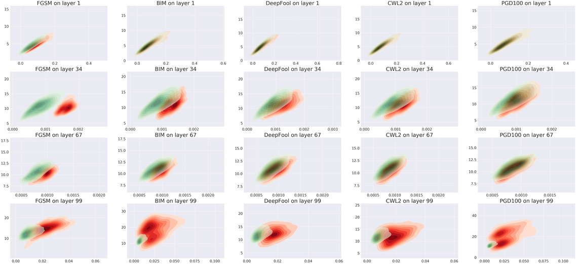
Below we provide the figures, which show normal and adversarial examples representations (their distributions). The figures are given for all six dataset-architecture combinations we explore. The normal (green) and adversarial (red) examples are visualized by the kernel density estimation in the 2D space. In each sub-figure, the x-axis is the reconstruction error, the y-axis is the $L_{2}$ norm in the latent space. Each column of sub-figures refers to a different attack (FGSM, BIM, Deepfool, Carlini-Wagner and PGD). The adversarial examples are followed through subsequent layers, each corresponding to a different row of sub-figures. In most investigated cases, the discrepancy between these distributions is most evident in last layers. However, for simpler attacks, such as FGSM, the adversarial examples can also be easily detected in earlier layers.

Figure 4: SVHN dataset, DenseNet model

Figure 5: SVHN dataset, ResNet model

Figure 6: CIFAR-10 dataset, DenseNet model

Figure 7: CIFAR-10 dataset, ResNet model

Figure 8: CIFAR-100 dataset, DenseNet model

Figure 9: CIFAR-100 dataset, ResNet model

Appendix B Significance of Adversarial Perturbation Magnitude

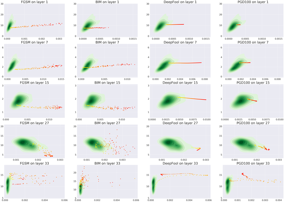
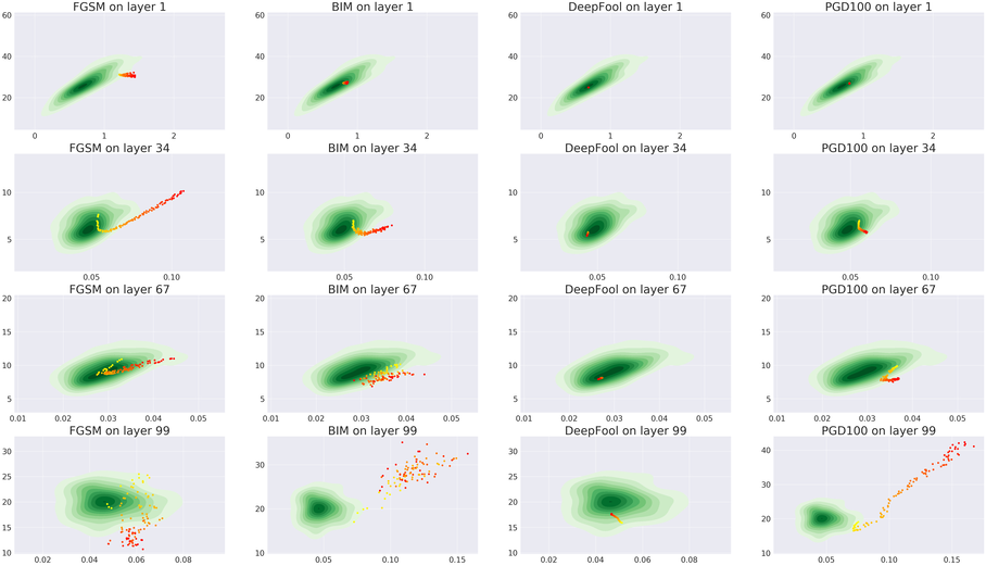
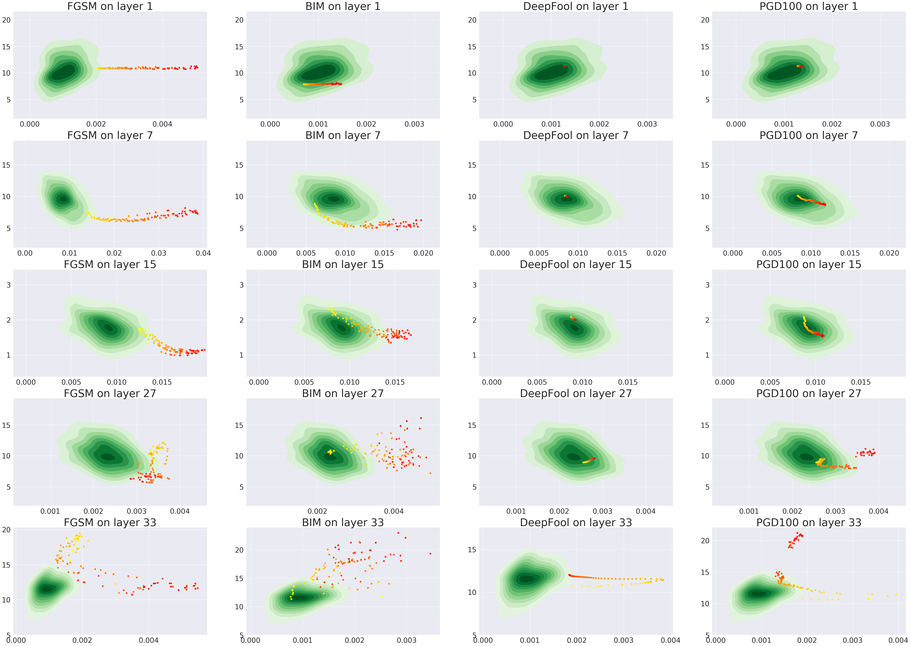
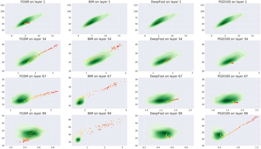
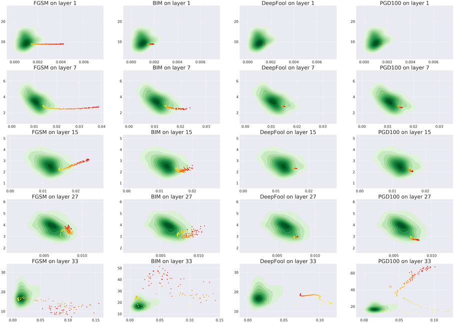
Below we provide the figures visualizing an impact of the perturbation magnitude on the position of an example in 2D space (reconstruction error in the x-axis and latent $L_{2}$ norm in the y-axis). The figures are given for all six dataset-architecture combinations we investigate.

The starting point is a single normal example without any perturbations (visualized as a light yellow dot). Then, we linearly increase the perturbation until it reaches the value of $2\epsilon$ (dark red). As a point of reference, we provide the kernel density estimation (green) of normal examples from the test set. Each column of sub-figures refers to a different attack (FGMS, BIM, DeepFool, PGD) and each row of sub-figures refers to a different layer. For most settings, we observe that adversarial examples significantly move away from the data manifold as the perturbation magnitude increases (movement in x-axis).

Figure 10: SVHN dataset, DenseNet model

Figure 11: SVHN dataset, ResNet model

Figure 12: CIFAR-10 dataset, DenseNet model

Figure 13: CIFAR-10 dataset, ResNet model

Figure 14: CIFAR-100 dataset, DenseNet model

Figure 15: CIFAR-100 dataset, ResNet model

Appendix C Layer importance

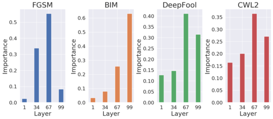
In this section we provide the layer importances calculated for the model with the random forest as the final classifier. Feature importances ($L_{2}$ norm in the latent space and the reconstruction error) are summed for a given layer. The final layers have the highest discriminative power except for the case of the simplest attack (FGSM), which can be easily detected using the activations from the second block of hidden layers. These findings are consistent with the figures from Section A.

Figure 16: CIFAR-100 dataset, DenseNet model

Figure 17: CIFAR-100 dataset, ResNet model

Figure 18: CIFAR-10 dataset, DenseNet model

Figure 19: CIFAR-10 dataset, ResNet model

Figure 20: SVHN dataset, DenseNet model

Figure 21: SVHN dataset, ResNet model

Appendix D Feature importance

We also investigate the feature importance for all dataset-architecture combinations with the random forest model. Features ($L_{2}$ norm in the latent space and the reconstruction error) are aggregated over layers. Clearly, the reconstruction error, which indicates the distance of a given sample from the manifold of true data, is more discriminative for detecting adversarial examples than the latent norm, which describes the movement within the manifold. This analysis supports Hypothesis 1 stated in the main body of the paper.

Figure 22: CIFAR-100 dataset, DenseNet model

Figure 23: CIFAR-100 dataset, ResNet model

Figure 24: CIFAR-10 dataset, DenseNet model

Figure 25: CIFAR-10 dataset, ResNet model

Figure 26: SVHN dataset, DenseNet model

Figure 27: SVHN dataset, ResNet model

Appendix E Comparison of different representations

The final classifier can be trained on different representations taken from the auto-encoders. We compare representation using the entire latent vector (full), with ones based on either reconstruction error only, or the latent norm only or both features. The results reported for the supervised (Table 2) confirm that: (1) reconstruction error is more discriminative than latent norm (2) full latent representation is only slightly better than using two AE features. For the unsupervised case (Table 3) we do not consider the full latent vectors as the one-class methods we examine perform poorly when the feature space is large. In the unsupervised setting the reconstruction error is also the most important feature.

Model	Dataset		FGSM	BIM	DeepFool	CW	PGD
DenseNet	CIFAR-10	full	100.00	99.99	91.36	97.75	99.61
		both	99.03	99.96	88.26	94.34	99.38
		rec. error	98.20	99.23	78.81	84.95	97.66
		lat. norm	88.32	99.52	78.58	86.08	97.75
	CIFAR-100	full	100.00	99.88	88.17	96.40	96.63
		both	99.94	99.60	81.63	88.25	97.26
		rec.error	99.71	99.50	73.32	78.97	96.92
		lat. norm	99.80	90.71	77.26	82.35	83.44
	SVHN	full	99.98	99.75	97.26	97.80	99.43
		both	99.93	98.77	95.24	96.98	97.20
		rec.error	99.40	96.12	91.75	92.54	95.81
		lat. norm	79.90	85.12	57.22	65.43	87.08
ResNet	CIFAR-10	full	99.98	99.61	86.41	95.01	97.39
		both	100.0	99.91	91.37	93.95	94.03
		rec.error	99.99	99.14	91.05	91.55	83.07
		lat. norm	92.87	97.95	64.41	78.11	90.66
	CIFAR-100	full	100.00	99.52	77.98	96.41	98.12
		both	99.98	98.52	85.00	95.08	96.62
		rec.error	99.98	98.52	81.02	92.05	78.59
		lat. norm	98.11	95.90	78.29	87.84	94.81
	SVHN	full	99.81	99.10	95.45	97.31	97.41
		both	99.95	99.56	96.33	98.01	93.86
		rec.error	99.92	99.29	95.78	97.48	88.30
		lat. norm	98.38	93.30	78.99	85.95	86.49

Table 2: Comparison of four variants of AE representations for supervised learning: (1) entire latent vector, (2) reconstruction error supplied with latent norm, (3) reconstruction error only (4) latent norm only.

Model	Dataset		FGSM	BIM	DeepFool	CW	PGD
DenseNet	CIFAR-10	both	78.38	97.51	65.31	68.15	94.20
		rec. error	82.87	95.79	65.28	70.35	91.88
		lat. norm	63.27	95.82	59.05	59.37	90.47
	CIFAR-100	both	97.95	95.68	61.86	62.28	87.19
		rec. error	96.98	96.92	59.74	59.81	91.30
		lat. norm	95.05	77.46	59.14	59.10	66.64
	SVHN	both	96.50	94.07	83.80	84.81	93.70
		rec. error	96.66	91.43	85.84	84.82	91.11
		lat. norm	69.88	82.19	56.61	61.81	84.58
ResNet	CIFAR-10	both	97.24	94.93	78.19	74.29	77.25
		rec. error	97.42	91.19	83.21	78.52	69.79
		lat. norm	70.91	90.34	46.24	49.82	75.34
	CIFAR-100	both	95.59	80.23	71.06	73.02	70.98
		rec. error	96.53	79.77	70.70	73.76	58.00
		lat. norm	71.94	69.45	61.18	60.62	76.67
	SVHN	both	98.90	95.49	89.36	90.02	83.62
		rec. error	99.09	95.78	90.84	91.76	80.34
		lat. norm	88.30	77.95	60.71	65.48	72.67

Table 3: Performance comparison of the one-class classifier (Isolation Forest) trained on: (1) reconstruction error and latent norm, (2) reconstruction error only, (3) latent norm only.

Appendix F Detection in the partially supervised scenario

We examine how the detector trained on the FGSM attack generalizes to other types of attacks. Table 4 shows that the performance of our method is comparable to the Mahalanobis detector (Lee et al., 2018). We argue that there might be a trade-off between performance on a fully supervised setting (where our method gets 100% on some cases) and a generalization ability to other attacks.

Model	Dataset	Method	FGSM (seen)	BIM	DeepFool	CW
DenseNet	CIFAR-10	Mahalanobis	99.94	99.51	83.42	87.95
		AE-layers (ours)	100.00	95.25	84.59	92.44
	CIFAR-100	Mahalanobis	99.86	98.27	75.63	86.20
		AE-layers (ours)	100.00	98.54	82.96	93.75
	SVHN	Mahalanobis	99.85	99.12	93.47	96.95
		AE-layers (ours)	99.98	96.94	87.55	93.45
ResNet	CIFAR-10	Mahalanobis	99.94	98.91	78.06	93.90
		AE-layers (ours)	99.98	91.53	70.82	88.19
	CIFAR-100	Mahalanobis	99.77	96.38	81.95	90.96
		AE-layers (ours)	100.00	94.02	73.53	93.82
	SVHN	Mahalanobis	99.62	95.39	72.20	86.73
		AE-layers (ours)	99.81	92.46	75.66	86.99

Table 4: Comparison of AUROC (%) scores. The classifier is trained on the FGSM attack and tested against other attacks. For our method, we use SVM as the final classifier and the entire latent vectors as its input features.

Appendix G Attack strength vs. detection performance

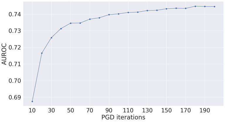
To investigate how the number of iterations in the PGD attack affects the detection performance, we generate adversarial examples for the entire test set for multiple iteration count values. We then measure the detection performance of our unsupervised Isolation Forest final classifier for each iteration value. We perform this experiment on CIFAR-10 and the ResNet architecture and present the results in Figure 28. Interestingly, the stronger attack (more iterations), the better detection performance. We observe similar phenomenon with the Odds-testing method (Roth et al., 2019) when ‘weaker’ attacks turn out to be much more challenging for that method (See Table 1 in the main body of the paper.) Full explanation of this observation could be interesting future work.

Figure 28: PGD iterations vs. detection performance

Appendix H Autoencoders architecture

We use the same hyperparameters for each autoencoder and if the representation size allows, the same architecture, even between datasets and models. Each encoder has 3 convolutional layers with 128 filters, the stride set to 2, ReLU activations and a single fully-connected layer with the latent size set to 64. The architectures of the decoder and the encoder are symmetric.

References

- Amodei et al. (2016) Amodei, D., Ananthanarayanan, S., Anubhai, R., Bai, J., Battenberg, E., Case, C., Casper, J., Catanzaro, B., Cheng, Q., Chen, G., et al. Deep speech 2: End-to-end speech recognition in english and mandarin. In International conference on machine learning, pp. 173–182, 2016.
- Carlini & Wagner (2017) Carlini, N. and Wagner, D. Adversarial examples are not easily detected: Bypassing ten detection methods. 2017.
- Carlini et al. (2017) Carlini, N., Katz, G., Barrett, C., and Dill, D. L. Provably minimally-distorted adversarial examples. arXiv preprint arXiv:1709.10207, 2017.
- Ehlers (2017) Ehlers, R. Formal verification of piece-wise linear feed-forward neural networks. In International Symposium on Automated Technology for Verification and Analysis, pp. 269–286. Springer, 2017.
- Fefferman et al. (2013) Fefferman, C., Mitter, S., and Narayanan, H. Testing the manifold hypothesis, 2013.
- Goodfellow et al. (2014) Goodfellow, I. J., Shlens, J., and Szegedy, C. Explaining and harnessing adversarial examples. arXiv preprint arXiv:1412.6572, 2014.
- Grosse et al. (2017a) Grosse, K., Manoharan, P., Papernot, N., Backes, M., and McDaniel, P. On the (statistical) detection of adversarial examples. arXiv preprint arXiv:1702.06280, 2017a.
- Grosse et al. (2017b) Grosse, K., Papernot, N., Manoharan, P., Backes, M., and McDaniel, P. Adversarial examples for malware detection. In European Symposium on Research in Computer Security, pp. 62–79. Springer, 2017b.
- He et al. (2016) He, K., Zhang, X., Ren, S., and Sun, J. Deep residual learning for image recognition. In Proceedings of the IEEE conference on computer vision and pattern recognition, pp. 770–778, 2016.
- Hendrycks & Gimpel (2016) Hendrycks, D. and Gimpel, K. A baseline for detecting misclassified and out-of-distribution examples in neural networks. arXiv preprint arXiv:1610.02136, 2016.
- Huang et al. (2017) Huang, G., Liu, Z., Van Der Maaten, L., and Weinberger, K. Q. Densely connected convolutional networks. In Proceedings of the IEEE conference on computer vision and pattern recognition, pp. 4700–4708, 2017.
- Kingma & Welling (2014) Kingma, D. P. and Welling, M. Auto-encoding variational bayes. In 2nd International Conference on Learning Representations, ICLR 2014, Banff, AB, Canada, April 14-16, 2014, Conference Track Proceedings, 2014. URL http://arxiv.org/abs/1312.6114.
- Krizhevsky et al. (a) Krizhevsky, A., Nair, V., and Hinton, G. Cifar-10 (canadian institute for advanced research). a. URL http://www.cs.toronto.edu/~kriz/cifar.html.
- Krizhevsky et al. (b) Krizhevsky, A., Nair, V., and Hinton, G. Cifar-100 (canadian institute for advanced research). b. URL http://www.cs.toronto.edu/~kriz/cifar.html.
- Kurakin et al. (2016) Kurakin, A., Goodfellow, I., and Bengio, S. Adversarial examples in the physical world. arXiv preprint arXiv:1607.02533, 2016.
- Lee et al. (2018) Lee, K., Lee, K., Lee, H., and Shin, J. A simple unified framework for detecting out-of-distribution samples and adversarial attacks. In Advances in Neural Information Processing Systems, pp. 7167–7177, 2018.
- Lomuscio & Maganti (2017) Lomuscio, A. and Maganti, L. An approach to reachability analysis for feed-forward relu neural networks. arXiv preprint arXiv:1706.07351, 2017.
- Madry et al. (2017) Madry, A., Makelov, A., Schmidt, L., Tsipras, D., and Vladu, A. Towards deep learning models resistant to adversarial attacks. arXiv preprint arXiv:1706.06083, 2017.
- Moosavi-Dezfooli et al. (2016) Moosavi-Dezfooli, S.-M., Fawzi, A., and Frossard, P. Deepfool: a simple and accurate method to fool deep neural networks. In Proceedings of the IEEE conference on computer vision and pattern recognition, pp. 2574–2582, 2016.
- Morawiecki et al. (2019) Morawiecki, P., Spurek, P., Śmieja, M., and Tabor, J. Fast and stable interval bounds propagation for training verifiably robust models. arXiv preprint arXiv:1906.00628, 2019.
- Netzer et al. (2011) Netzer, Y., Wang, T., Coates, A., Bissacco, A., Wu, B., and Ng, A. Y. Reading digits in natural images with unsupervised feature learning. In NIPS Workshop on Deep Learning and Unsupervised Feature Learning 2011, 2011. URL http://ufldl.stanford.edu/housenumbers/nips2011_housenumbers.pdf.
- Papernot & McDaniel (2018) Papernot, N. and McDaniel, P. D. Deep k-nearest neighbors: Towards confident, interpretable and robust deep learning. CoRR, abs/1803.04765, 2018. URL http://arxiv.org/abs/1803.04765.
- Pidhorskyi et al. (2018) Pidhorskyi, S., Almohsen, R., and Doretto, G. Generative probabilistic novelty detection with adversarial autoencoders. In Advances in neural information processing systems, pp. 6822–6833, 2018.
- Roth et al. (2019) Roth, K., Kilcher, Y., and Hofmann, T. The odds are odd: A statistical test for detecting adversarial examples. arXiv preprint arXiv:1902.04818, 2019.
- Samangouei et al. (2018) Samangouei, P., Kabkab, M., and Chellappa, R. Defense-gan: Protecting classifiers against adversarial attacks using generative models. arXiv preprint arXiv:1805.06605, 2018.
- Sitawarin et al. (2018) Sitawarin, C., Bhagoji, A. N., Mosenia, A., Chiang, M., and Mittal, P. Darts: Deceiving autonomous cars with toxic signs. arXiv preprint arXiv:1802.06430, 2018.
- Szegedy et al. (2013) Szegedy, C., Zaremba, W., Sutskever, I., Bruna, J., Erhan, D., Goodfellow, I., and Fergus, R. Intriguing properties of neural networks. arXiv preprint arXiv:1312.6199, 2013.
- Tabor et al. (2018) Tabor, J., Knop, S., Spurek, P., Podolak, I., Mazur, M., and Jastrzębski, S. Cramer-wold autoencoder. arXiv preprint arXiv:1805.09235, 2018.
- Tolstikhin et al. (2018) Tolstikhin, I. O., Bousquet, O., Gelly, S., and Schölkopf, B. Wasserstein auto-encoders. In 6th International Conference on Learning Representations, ICLR 2018, Vancouver, BC, Canada, April 30 - May 3, 2018, Conference Track Proceedings, 2018.
- Xiao et al. (2018) Xiao, K. Y., Tjeng, V., Shafiullah, N. M., and Madry, A. Training for faster adversarial robustness verification via inducing relu stability. arXiv preprint arXiv:1809.03008, 2018.
- Xu et al. (2017) Xu, W., Evans, D., and Qi, Y. Feature squeezing: Detecting adversarial examples in deep neural networks. arXiv preprint arXiv:1704.01155, 2017.
- Yang et al. (2019) Yang, P., Chen, J., Hsieh, C.-J., Wang, J.-L., and Jordan, M. I. Ml-loo: Detecting adversarial examples with feature attribution. arXiv preprint arXiv:1906.03499, 2019.
- Zhang et al. (2018) Zhang, H., Weng, T.-W., Chen, P.-Y., Hsieh, C.-J., and Daniel, L. Efficient neural network robustness certification with general activation functions. In Advances in Neural Information Processing Systems, pp. 4939–4948, 2018.
- Zhao et al. (2019) Zhao, Z.-Q., Zheng, P., Xu, S.-t., and Wu, X. Object detection with deep learning: A review. IEEE transactions on neural networks and learning systems, 30(11):3212–3232, 2019.