Simulating cosmological supercooling with a cold atom system

Abstract

We perform an analysis of the supercooled state in an analogue to an early universe phase transition based on a one dimensional, two-component Bose gas. We demonstrate that the thermal fluctuations in the relative phase between the components are characteristic of a relativistic thermal system. Furthermore, we demonstrate the equivalence of two different approaches to the decay of the metastable state: specifically a non-perturbative thermal instanton calculation and a stochastic Gross–Pitaevskii simulation.

I Introduction

In its early stages, our universe was filled with hot, relativistic plasma that cooled through all of the major energy thresholds of fundamental particle physics, undergoing several changes of phase between different physical regimes. At the most extreme, the universe may have undergone first order transitions, characterised by metastable, supercooled states and the nucleation of bubbles. Bubbles of a new matter phase would produce huge density variations, and unsurprisingly first order phase transitions have been proposed as sources of gravitational waves Caprini et al. (2009); Hindmarsh et al. (2014) and as sources of primordial black holes Hawking et al. (1982); Deng and Vilenkin (2017). Despite the importance of this phenomenon, we have no experimental test of the basic theory. In this paper, we propose that a thermal supercooled state, analogous to a relativistic system, can be realised in a Bose gas experiment.

Phase transitions in fundamental particle physics can be associated with a Klein-Gordon field in an effective potential. At high temperatures, the field fluctuates about the minimum value of the potential representing a high temperature phase. As the temperature drops, the minimum of the potential changes to represent the low temperature phase, but the field can become trapped in a metastable state. Extreme supercooling can even lead to a zero-temperature metastable ‘false vacuum’ state.

The idea of using analogue systems for cosmological processes comes under the general area of modelling the “universe in the laboratory” Roger et al. (2016); Eckel et al. (2018). So far, analogue systems have mostly been employed to test ideas in perturbative quantum field theory Unruh (1981); Barcelo et al. (2005), but the non-perturbative phenomenon of false vacuum decay has recently been discussed, with theoretical descriptions of vacuum decay of atomic Braden et al. (2019a) and relativistic systems Braden et al. (2019b) at zero temperatures. Among possible analogue systems, (quasi-)one-dimensional ultracold Bose gases have emerged as an outstandingly versatile experimental platform for probing many-body quantum dynamics Langen et al. (2015); Erne et al. (2018); Prüfer et al. (2018).

Fialko et al. Fialko et al. (2015, 2017) proposed an actual experiment to simulate the relativistic vacuum decay in a cold atom system. Their system consists of a Bose gas with two different spin states of the same atom species in an optical trap. The two states are coupled by a microwave field. By modulating the amplitude of the microwave field, a new quartic interaction between the two states is induced in the time-averaged theory which creates a non-trivial ground state structure as illustrated in Fig. 1.

In this paper we introduce thermal effects into the model of Fialko et al. to better replicate the conditions relevant to the very early universe. We take their time-averaged potential and study the physics of supercooling for a metastable state in the thermal “cross-over” regime of a quasi-one-dimensional Bose gas. We demonstrate the bubble nucleation dynamics of the first order phase transition are correctly reproduced by numerical modelling using a stochastic projected Gross–Pitaevskii equation (SPGPE) Gardiner et al. (2002); Gardiner and Davis (2003); Bradley et al. (2008); Blakie et al. (2008); Bradley and Blakie (2014). We show that the stochastic approach agrees with semi-classical predictions based on non-equilibrium thermal field theory of a relativistic Klein Gordon system. This agreement applies not only to the correlation functions, but also to the non-perturbative decay rate of a metastable state.

This paper also sets up further work extending the results to oscillating potentials which we hope to present in due course. Braden et al. have shown that oscillating potentials lead to a parametric instability on small wavelengths which causes a classical decay of the metastable state Braden et al. (2018, 2019b). In order to produce a supercooled system, some form of dissipative mechanism would have to act on small scales to damp out the parametric resonance, and we propose that thermal damping may be the solution.

Figure 1: The field potential $V$ plotted as a function of the relative phase of the two atomic wave functions, $\varphi$. The metastable phase is at the minimum $\varphi=\pi$ and the stable phase is at the global minimum $\varphi=0$. The difference in energy density between these phases is $\Delta V$.

II System

Our system is a one-dimensional, two-component Bose gas of atoms with mass $m$. The two components are different spin states of the same species, coupled by a time-modulated microwave field. The Hamiltonian is given by

$$H=\int dx\left\{-{\hbar^{2}\over 2m}\psi^{\dagger}\nabla^{2}\psi+V(\psi,\psi^{\dagger})\right\},$$ (1)

where the field operator $\psi$ has two components $\psi_{i}$, $i=1,2$. Fialko et al. Fialko et al. (2015, 2017) described a procedure whereby averaging over timescales longer than the modulation timescale can lead to an interaction potential of the form

$$V=\frac{g}{2}\sum_{i}\left(\psi_{i}^{\dagger}\psi_{i}\right)^{2}-\mu\psi^{\dagger}\psi-\mu\epsilon^{2}\psi^{\dagger}\sigma_{x}\psi+\frac{g}{4}\epsilon^{2}\lambda^{2}(\psi^{\dagger}\sigma_{y}\psi)^{2},$$ (2)

where $\sigma_{\{x,y\}}$ are Pauli matrices. The potential includes the chemical potential $\mu$, equal intra-component $s$-wave interactions of strength $g$ between the field operators (we assume inter-component $s$-wave interactions are negligible), and a microwave-induced interaction with strength $\mu\epsilon^{2}$. The final term comes from the averaging procedure, and introduces a new parameter $\lambda$, dependent on the amplitude of the modulation. The trapping potential used to confine the condensate has been omitted in order to isolate the physics of vacuum decay. In principle, a quasi-one-dimensional ring trap experiment could realize the uniform system we study.

The terms proportional to $\epsilon^{2}$ are responsible for the difference in energy between the global and local minima of the energy, and we require $\epsilon$ to be small. The global minimum represents the true vacuum state and the local minimum represents the false vacuum. The true vacuum is a state with $\psi_{1}=\psi_{2}$ and the false vacuum is a state with $\psi_{1}=-\psi_{2}$. The condensate densities of the two components at the extrema are equal to one another, and given by $\langle\psi_{1}^{\dagger}\psi_{1}\rangle=\langle\psi_{2}^{\dagger}\psi_{2}\rangle=\rho_{0}(1\pm\epsilon^{2})$, in terms of the mean density $\rho_{0}=\mu/g$.

Throughout this paper, we will make use of the healing length $\xi=\hbar/(mg\rho_{0})^{1/2}$ and the sound speed $c=\hbar/(m\xi)$. Together, these define a characteristic frequency $\omega_{0}=c/\xi$. The dimensionless form of the potential constructed from these parameters becomes $\hat{V}=V/(\hbar\omega_{0}\rho_{0})$. If we now introduce the relative phase $\varphi$ between the spin components, such that $\psi_{1}\approx\rho_{0}e^{i\varphi/2}$ and $\psi_{2}\approx\rho_{0}e^{-i\varphi/2}$, then the potential becomes

$$\hat{V}\approx-2\epsilon^{2}-2\epsilon^{2}\cos\varphi+\epsilon^{2}\lambda^{2}\sin^{2}\varphi,$$ (3)

as shown in Fig. 1, with $\Delta V=4\hbar\omega_{0}\rho_{0}\epsilon^{2}$.

In the experimental proposal, the system is initially prepared in the metastable phase at a temperature $T$. In one dimension, the physics of Bose gases critically depends on the dimensionless interaction strength parameter $\zeta=(\rho_{0}\xi)^{-2}$ and the temperature Kheruntsyan et al. (2003, 2005); Bouchoule et al. (2012); Henkel et al. (2017). We consider the weakly interacting case, $\zeta\ll 1$. A phase-fluctuating quasi-condensate, in which density fluctuations are suppressed, appears at temperatures below the cross-over temperature

$$T_{CO}={\hbar c\rho_{0}\over k_{B}}.$$ (4)

The gas remains degenerate up to a temperature of order $T_{D}=\zeta^{-1/2}T_{CO}>T_{CO}$.

III Stochastic Gross Pitaevskii equation

Stochastic Gross–Pitaevskii equations (SGPEs) are widely used for modeling atomic gases at and below the condensation temperature Stoof (1999); Stoof and Bijlsma (2001); Gardiner et al. (2002); Gardiner and Davis (2003); Bradley et al. (2008); Blakie et al. (2008). Here, we use the simple growth stochastic projected Gross–Pitaevskii equation (SPGPE) Bradley et al. (2008); Blakie et al. (2008), which has been successfully used to model experimental phase transitions Weiler et al. (2008); Liu et al. (2018). Extension of the SPGPE to spinor and multi-component condensates is described in Ref. Bradley and Blakie (2014).

For convenience, from this point in the paper we use $\xi$ as the length unit and $\omega_{0}^{-1}$ as the time unit. We also rescale the wave function by replacing $\psi\to\rho_{0}^{1/2}\psi$, and measure the temperature in units of $T_{CO}$. In these units, the form of SPGPE we use is

$$i{\partial\psi_{j}\over\partial t}={\cal P}\left\{(1-i\gamma)\left(-\frac{1}{2}\nabla^{2}\psi_{j}+{\partial\hat{V}\over\partial\psi_{j}^{\dagger}}\right)+\eta_{j}\right\}.$$ (5)

Here the complex fields $\psi_{j}$ describe the well-occupied, low-momentum modes of the system (the c-field region), and the projector $\mathcal{P}$ eliminates modes above the momentum cut-off $k_{\mathrm{cut}}=\sqrt{2\rho_{0}\xi T}$. We also considered other values of $k_{\textrm{cut}}$, to ensure our results were not overly sensitive to the choice of momentum cut-off. The noise source $\eta$ is a Gaussian random field with correlation function

$$\langle\eta_{i}(x,t)\eta_{j}(x^{\prime},t^{\prime})\rangle=2\gamma T\delta(x-x^{\prime})\delta(t-t^{\prime})\delta_{ij},$$ (6)

and the potential

$$\hat{V}=\frac{1}{2}\sum_{i}\left(\psi_{i}^{\dagger}\psi_{i}-1\right)^{2}-\epsilon^{2}\psi^{\dagger}\sigma_{x}\psi+\frac{1}{4}\lambda^{2}\epsilon^{2}(\psi^{\dagger}\sigma_{y}\psi)^{2}.$$ (7)

Typically, we set the dimensionless dissipation rate $\gamma=10^{-2}$. Values of $\gamma$ from $\mathcal{O}(10^{-4})$ to $\mathcal{O}(10^{-2})$ have been used in previous work that made direct comparisons to experiment Weiler et al. (2008); Rooney et al. (2013); Ota et al. (2018); Liu et al. (2018), making this a reasonable choice. We comment on the effect of $\gamma$ later in the text. Our SPGPE simulations use a one dimensional grid of size $L=240\xi$ with periodic boundaries and spacing $\Delta x=0.4\xi$. We set $\rho_{0}\xi=100$. Our simulations were executed using the software package XMDS2 Dennis et al. (2013). Averaged quantities were calculated over $1000$ stochastic realizations.

Some care should be exercised when applying the SPGPE in reduced dimensions, since a three-dimensional thermal cloud is assumed Bradley et al. (2015). For a gas confined in a transverse harmonic trap of frequency $\omega_{\perp}$, the simple growth SPGPE above is valid in 1D with dimensionally-reduced interaction strength $g=2\hbar a_{s}\omega_{\perp}$ provided $\hbar\omega_{\perp}\lesssim k_{\mathrm{B}}T$ and, in principle, $\mu\ll\hbar\omega_{\perp}$. In practice $\mu\lesssim\hbar\omega_{\perp}$ is sufficient: 1D S(P)GPE equilibrium states were investigated in Refs. Cockburn et al. (2011); Davis et al. (2012) and shown to be an excellent match to quasi-1D atom-chip experiments in this regime Trebbia et al. (2006); van Amerongen et al. (2008).

We will be running at some fraction of the cross-over temperature $T_{CO}$ which is larger than the temperature, $T_{\phi}=\hbar^{2}\rho_{0}/(mk_{\mathrm{B}}L)$, at which phase coherence is attained across the entire system Crucially however, the relative phase $\varphi$ has an effective potential barrier that assists phase coherence in the relative phase at higher temperatures than $T_{\phi}$, as we shall see in the following results.

Figure 2: The correlation function for the relative phase, $g(|x-x^{\prime}|)=\langle\varphi(x,t)\varphi(x^{\prime},t)\rangle$, at different temperatures in a potential with $\lambda=1.4$ and $\epsilon=0.1$. The SPGPE results agree with the correlations of a thermal Klein Gordon field at the lower temperatures, but non-linear effects start to cause a difference as the temperature increases. Nonetheless, better agreement can be achieved at higher temperatures by fitting an effective value of $\lambda_{\mathrm{eff}}$ at each temperature (inset).

IV Results

IV.1 Equilibrium correlations

The correlation functions for fluctuations about the stable and metastable phases provide an essential check on the validity of the numerical modelling, and also elucidates the relation between fluctuations in the SGPE and the Klein-Gordon field $\varphi$. As shown in Appendix A, small fluctuations in the relative phase $\varphi$ of the two components induced by the SGPE have a thermal Klein Gordon correlation function

$$\langle\varphi(x,t)\varphi(x^{\prime},t)\rangle={T\over m_{\varphi}}e^{-m_{\varphi}|x-x^{\prime}|}+{T\over 2}\delta(x-x^{\prime}),$$ (8)

where the Klein-Gordon mass $m_{\varphi}=2\epsilon(\lambda^{2}\pm 1)^{1/2}$, for the stable and metastable phases respectively.

The correlation function about the stable phase computed from SPGPE simulations is shown in Fig. 2. As expected, at low temperatures we have complete agreement with the Klein-Gordon result. At higher temperatures, non-linear effects are increasingly important, until the state becomes completely phase incoherent, in analogy to symmetry restoration in fundamental particle physics. At intermediate temperatures, we can restore the agreement against the theoretical result by introducing an ‘effective’ coupling’ $\lambda_{\rm eff}$, as shown in the inset in Fig. 2.

IV.2 Bubble nucleation

In a first order regime, we expect to see exponential decay of the metastable state, triggered by bubble nucleation events. In this section we present numerical results which confirm this prediction, and we show agreement with a semi-classical, non-perturbative instanton approach.

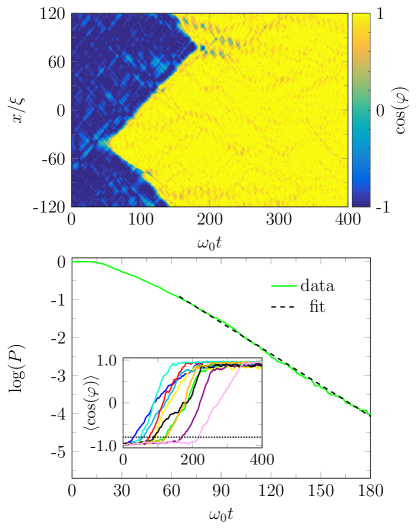
Figure 3: Above, an example of bubble nucleation for $\lambda=1.4$ and $T=0.03T_{CO}$. Below, the logarithm of the probability, $P$, of remaining in the metastable state. In this case the system was first allowed to equilibrate at $\lambda=1.8$, a barrier large enough that bubble nucleation was negligible, after which the barrier was reduced to $\lambda=1.4$. Inset, the spatial average of $\cos\varphi$ for ten different runs. The nucleation time is taken to be when $\langle\cos\varphi\rangle>-1+\Delta$, where $\Delta=0.2$ in this example.

In order to model bubble nucleation using the the SPGPE, we must initialize the system in the metastable state. In most runs we do this by placing the fields $\psi_{j}$ in the fluctuation-free metastable state at time $t=0$, allowing the noise term in the SPGPE [Eq. (5)] to rapidly build up thermal fluctuations. We also verified that equivalent results are produced by first allowing the fields to thermalize with a high potential barrier ($\lambda=1.8$) and then instantaneously reducing $\lambda$, since this latter procedure is closer to a likely experimental protocol. A signature of bubble formation in an individual trajectory is given by the spatial average $\langle\cos\varphi\rangle$ exceeding $-1+\Delta$, where $\Delta=0.2$ is chosen to be larger than the typical fluctuations of $\langle\cos\varphi\rangle$ due to thermal noise in the system. An example is shown in Fig. 3. Running many stochastic trajectories and computing the probability, $P$, of remaining in the metastable state results in an exponential decay curve, also shown in Fig. 3. A fit to the exponential form $P=ae^{-\Gamma t}$ over the time intervals seen to be exhibiting exponential decay yields the decay rate $\Gamma$. Figure 4 shows the decay rate $\Gamma$ for several values of $T$ and $\lambda$. Uncertainties on $\Gamma$, reflecting the statistical uncertainty arising from the trajectory averaging, are computed by a bootstrap resampling approach Billam et al. (2019).

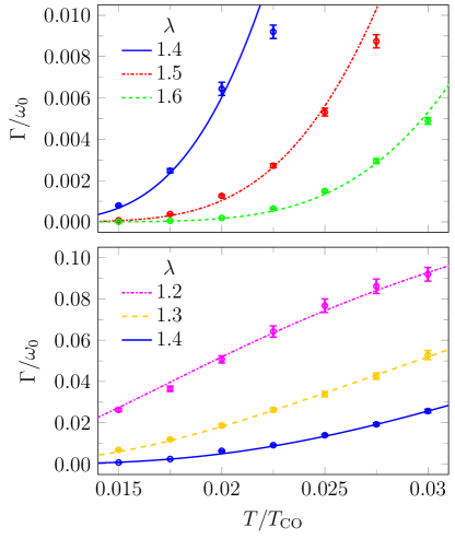
Figure 4: A comparison between the decay constant obtained from the SPGPE (data points) and the instanton method (lines) as a function of temperature. These plots are for $\epsilon=0.1$, interaction strength $\zeta=10^{-4}$ and dissipation $\gamma=10^{-2}$. There is good agreement when the decay constant $\Gamma<\gamma$, and this can be extended to higher $\Gamma$ by using an effective coupling $\lambda_{\rm eff}$ (lower plot).

The semi-classical model of bubble decay is based on an instanton calculation, where the equations are solved in imaginary time $\tau$ to give an instanton solution $\psi_{b}$. For thermal scenarios, the imaginary time coordinate is taken to be periodic, with period $\beta=\hbar/(k_{B}T)$. The instanton solution approaches the metastable state at large distances, and for a purely thermal transition the solution is independent of $\tau$.

The full expression for the nucleation rate of vacuum bubbles in a volume ${\cal V}$ is Coleman (1977); Callan and Coleman (1977),

$$\Gamma\approx{\cal V}A_{0}B^{1/2}e^{-B}.$$ (9)

where $B$ denotes the difference in action between the instanton and the metastable state divided by $\hbar$. The pre-factor $A_{0}$ depends on the change in the spectra of the perturbative modes induced by the instanton. This should only depend mildly on temperature, so we will treat this term as an undetermined constant.

The exponent is explicitly

$$B=\rho_{0}\int_{-\infty}^{\infty}dx\int_{0}^{\beta}d\tau\left\{\psi_{b}^{\dagger}{\partial\psi_{b}\over\partial\tau}+\frac{1}{2}\psi_{b}^{\dagger}\nabla^{2}\psi_{b}+\hat{V}\right\}.$$ (10)

In the Klein-Gordon approximation, the decay exponent simplifies to

$$B={\alpha(\lambda)\epsilon\over T},$$ (11)

where the factor $\alpha(\lambda)$ is defined by

$$\alpha(\lambda)={1\over 4\epsilon}\int_{-\infty}^{\infty}dx\left\{\left({\partial\varphi_{b}\over\partial x}\right)^{2}+4\hat{V}\right\}.$$ (12)

Note that the $\epsilon$ dependence in (12) disappears if we rescale $x\to x/\epsilon$ and use Eq. (3).

The values of $\alpha(\lambda)$ for a Klein-Gordon model have been obtained recently in Ref. Gutierezz Abed and Moss . A comparison between the instanton and stochastic approaches is shown in Fig. 4. They agree very well in the region were $\Gamma<\gamma$, which we interpret as the nucleation rate having to be less that the relaxation rate of the thermal ensemble. Remarkably, the two approaches also agree over a wider range if we replace the coupling $\lambda$ by an ‘effective’ value $\lambda_{\rm eff}$.

Finally, we note that we repeated a sample of our SPGPE simulations with lower dissipation rate $\gamma=5\times 10^{-3}$. We find that the rate $\Gamma$ is dependent on $\gamma$. However, the results are still well-fitted by the instanton approach, but with a different pre-factor $A_{0}$, as would be expected from the theory of dissipative tunnelling in quantum mechanics Caldeira and Leggett (1981).

V Conclusion

The quasi-condensed thermal Bose gas described above would serve as a laboratory analogue to an early universe, supercooled phase transition. We show that the SPGPE can be used to model the system, and that where overlap with instanton calculations is possible there is agreement between the predictions of the two approaches.

As an example experimental configuration, we consider one of the experimental setups proposed by Fialko et al. Fialko et al. (2017), which is based on tuning the interactions between two Zeeman states of ${}^{7}{\rm Li}$ . The interactions can be tuned using a Feshbach resonance to achieve the required close-to-zero inter-component scattering length Fialko et al. (2017). Based on the average intra-component scattering length, suitable experimental parameters would be $5\times 10^{4}$ atoms in a quasi-1D optical trap Salces-Carcoba et al. (2018) of length $90\text{\,}\mathrm{\SIUnitSymbolMicro}\mathrm{m}$ and transverse frequency $2\pi\times$66\text{\,}\mathrm{k}\mathrm{H}\mathrm{z}$$. The interaction strength $\zeta=10^{-4}$ (as in Fig. 4), and the cross-over temperature $T_{CO}=$215\text{\,}\mathrm{\SIUnitSymbolMicro}\mathrm{K}$$. In this context the results in Fig. 4 correspond to temperatures from around $3.2\text{\,}\mathrm{\SIUnitSymbolMicro}\mathrm{K}$ to $6.4\text{\,}\mathrm{\SIUnitSymbolMicro}\mathrm{K}$, where bubble nucleation should be observable.

Interestingly, the phase correlation length at the temperatures of interest is less than the length of the gas, but the relative phase correlation length is larger than the system. This is because the phase of an individual atom is not constrained by the interactions; in the language of particle physics it is a ‘Goldstone mode’. On the other hand, the relative phase develops a potential and behaves as a massive Klein-Gordon field with correlation length fixed by the mass, as shown in Figure 2.

In future work, we will investigate a modulated (i.e., time varying) potential in order to investigate the effects of thermal damping on parametric instabilities. The semi-classical model of bubble nucleation used here is no longer applicable for a modulated potential, but the SPGPE will apply provided that $k_{B}T$ is larger than the maximum energy per mode $\hbar\omega_{k}$. Parametric resonance sets in on wavelengths a little less than the correlation length $\xi$ Braden et al. (2018, 2019b), and $k_{B}T>\hbar\omega_{k}$ in the parameter ranges discussed in the present paper. The parametric resonance has a fixed growth rate and it will be damped out given sufficiently large thermal damping. It is important to determine the exact degree of thermal damping required to see if this is physically realistic.

Also in future work, we will extend our results to two dimensions and include realistic trapping potentials. There is a possibility that the boundaries of the trap affect bubble nucleation, as we found in Billam et al. (2019), and this requires further theoretical investigation before two-dimensional simulations of vacuum decay and supercooling are constructed.

Data supporting this publication is openly available under a Creative Commons CC-BY-4.0 License on the data.ncl.ac.uk site Billam et al. (2020).

Appendix A Klein-Gordon reduction of the SGPE

Reduction to a Klein-Gordon system starts from

$$\psi_{1} =e^{\chi/2}e^{\sigma/2}e^{i\varphi/2}e^{i\theta/2},$$ (13)

$$\psi_{2} =e^{\chi/2}e^{-\sigma/2}e^{-i\varphi/2}e^{i\theta/2},$$ (14)

in an approximation where $\chi$, $\sigma$, $\nabla$ and $\partial_{t}$ are all $O(\epsilon)$. When these are inserted into Eq. (5) of the main text, the system reduces at leading order in $\epsilon$ to

$$\dot{\varphi} =-2\sigma+\eta_{\varphi},$$ (15)

$$\dot{\sigma} =-\frac{1}{2}\nabla^{2}\varphi-2\gamma\sigma+\partial_{\varphi}\hat{V}+\eta_{\sigma},$$ (16)

$$\dot{\theta} =-2\chi+\eta_{\theta},$$ (17)

$$\dot{\chi} =-\frac{1}{2}\nabla^{2}\theta-2\gamma\chi+\eta_{\chi},$$ (18)

where the noise terms have a gaussian distribution with covariance $2\gamma T$.

For small $\varphi$, these are a set of stochastic equations for the Bogliubov modes. In this limit, with $\hat{V}=m_{\varphi}^{2}\varphi^{2}/4$, they can be solved using green function techniques. The linearised equations for the transforms $\hat{\varphi}(k,\omega)$ and $\hat{\sigma}(k,\omega)$ are

$$\begin{pmatrix}-i\omega&2\\ -\omega_{k}^{2}/2&-i\omega+2\gamma\\ \end{pmatrix}\begin{pmatrix}\hat{\varphi}\\ \hat{\sigma}\\ \end{pmatrix}=\begin{pmatrix}\hat{\eta}_{\varphi}\\ \hat{\eta}_{\sigma}\end{pmatrix},$$ (19)

where $\omega_{k}^{2}=k^{2}+m_{\varphi}^{2}$. The inverse of the operator matrix is the Green function $G$,

$$G={1\over\Delta}\begin{pmatrix}i\omega-2\gamma&2\\ -\omega_{k}^{2}/2&i\omega\\ \end{pmatrix}\begin{pmatrix}\hat{\varphi}\\ \hat{\sigma}\\ \end{pmatrix},$$ (20)

where $\Delta=\omega^{2}+2i\gamma\omega-\omega_{k}^{2}$. The stochastic correllator of the relative phase fluctuations is related to the Green function by

$$\langle\hat{\varphi}(k,\omega)\hat{\varphi}(k^{\prime},\omega^{\prime})\rangle=\delta_{\omega\omega^{\prime}}\delta_{kk^{\prime}}2\gamma T\left(G_{\varphi\varphi}G_{\varphi\varphi}^{*}+G_{\varphi\sigma}G_{\varphi\sigma}^{*}\right)$$ (21)

Inverting the Fourier transform in $t$ gives the phase space correllator

$$\langle\hat{\varphi}(k,t)\hat{\varphi}^{*}(k^{\prime},t)\rangle={4+\omega_{k}^{2}\over 2\omega_{k}^{2}}T\delta_{kk^{\prime}}.$$ (22)

The first term in the denominator reproduces the thermal correllator for a free Klein Gordon field, which has energy of $T$ per Fourrier mode. In position space,

$$\langle\varphi(x,t)\varphi(x^{\prime},t)\rangle={T\over m_{\varphi}}e^{-m_{\varphi}r}+{T\over 2}\delta(r),$$ (23)

where $r=|x-x^{\prime}|$. The mass is given by $m_{\varphi}=2\epsilon(\lambda^{2}\pm 1)^{1/2}$ for the stable and metastable states respectively.

The result is valid for linearised theory. Including higher order terms makes a difference at higher temperature. The next order in perturbation theory introduces $T^{2}$ terms, or using re-summation modifies the mass $m_{\varphi}^{2}\to m_{\varphi}^{2}+\kappa T$, where $\kappa$ depends on regularisation.

References

- Caprini et al. (2009) C. Caprini, R. Durrer, T. Konstandin, and G. Servant, Phys. Rev. D79, 083519 (2009), arXiv:0901.1661 [astro-ph.CO] .
- Hindmarsh et al. (2014) M. Hindmarsh, S. J. Huber, K. Rummukainen, and D. J. Weir, Phys. Rev. Lett. 112, 041301 (2014), arXiv:1304.2433 [hep-ph] .
- Hawking et al. (1982) S. W. Hawking, I. G. Moss, and J. M. Stewart, Phys. Rev. D26, 2681 (1982).
- Deng and Vilenkin (2017) H. Deng and A. Vilenkin, JCAP 1712, 044 (2017), arXiv:1710.02865 [gr-qc] .
- Roger et al. (2016) T. Roger, C. Maitland, K. Wilson, N. Westerberg, D. Vocke, E. M. Wright, and D. Faccio, Nature Communications 7 (2016), 10.1038/ncomms13492.
- Eckel et al. (2018) S. Eckel, A. Kumar, T. Jacobson, I. B. Spielman, and G. K. Campbell, Phys. Rev. X8, 021021 (2018), arXiv:1710.05800 [cond-mat.quant-gas] .
- Unruh (1981) W. G. Unruh, Phys. Rev. Lett. 46, 1351 (1981).
- Barcelo et al. (2005) C. Barcelo, S. Liberati, and M. Visser, Living Rev. Rel. 8, 12 (2005), [Living Rev. Rel.14,3(2011)], arXiv:gr-qc/0505065 [gr-qc] .
- Braden et al. (2019a) J. Braden, M. C. Johnson, H. V. Peiris, A. Pontzen, and S. Weinfurtner, JHEP 10, 174 (2019a), arXiv:1904.07873 [hep-th] .
- Braden et al. (2019b) J. Braden, M. C. Johnson, H. V. Peiris, A. Pontzen, and S. Weinfurtner, Phys. Rev. Lett. 123, 031601 (2019b), arXiv:1806.06069 [hep-th] .
- Langen et al. (2015) T. Langen, S. Erne, R. Geiger, B. Rauer, T. Schweigler, M. Kuhnert, W. Rohringer, I. E. Mazets, T. Gasenzer, and J. Schmiedmayer, Science 348, 207 (2015), arXiv:1411.7185 [cond-mat.quant-gas] .
- Erne et al. (2018) S. Erne, R. Bücker, T. Gasenzer, J. Berges, and J. Schmiedmayer, Nature 563, 225 (2018), arXiv:1805.12310 [cond-mat.quant-gas] .
- Prüfer et al. (2018) M. Prüfer, P. Kunkel, H. Strobel, S. Lannig, D. Linnemann, C.-M. Schmied, J. Berges, T. Gasenzer, and M. K. Oberthaler, Nature 563, 217 (2018), arXiv:1805.11881 [cond-mat.quant-gas] .
- Fialko et al. (2015) O. Fialko, B. Opanchuk, A. I. Sidorov, P. D. Drummond, and J. Brand, EPL (Europhysics Letters) 110, 56001 (2015), arXiv:1408.1163 [cond-mat.quant-gas] .
- Fialko et al. (2017) O. Fialko, B. Opanchuk, A. I. Sidorov, P. D. Drummond, and J. Brand, Journal of Physics B Atomic Molecular Physics 50, 024003 (2017), arXiv:1607.01460 [cond-mat.quant-gas] .
- Gardiner et al. (2002) C. W. Gardiner, J. R. Anglin, and T. I. A. Fudge, Journal of Physics B: Atomic, Molecular and Optical Physics 35, 1555 (2002), arXiv:0112129 [cond-mat] .
- Gardiner and Davis (2003) C. W. Gardiner and M. J. Davis, Journal of Physics B: Atomic, Molecular and Optical Physics 36, 4731 (2003), arXiv:0308044 [cond-mat] .
- Bradley et al. (2008) A. S. Bradley, C. W. Gardiner, and M. J. Davis, Phys. Rev. A 77, 033616 (2008), arXiv:1804.04032 [cond-mat.quant-gas] .
- Blakie et al. (2008) P. Blakie, A. Bradley, M. Davis, R. Ballagh, and C. Gardiner, Advances in Physics 57, 363 (2008), arXiv:0809.1487 [cond-mat.quant-gas] .
- Bradley and Blakie (2014) A. S. Bradley and P. B. Blakie, Phys. Rev. A 90, 023631 (2014), arXiv:1406.2029 [cond-mat.quant-gas] .
- Braden et al. (2018) J. Braden, M. C. Johnson, H. V. Peiris, and S. Weinfurtner, JHEP 07, 014 (2018), arXiv:1712.02356 [hep-th] .
- Kheruntsyan et al. (2003) K. V. Kheruntsyan, D. M. Gangardt, P. D. Drummond, and G. V. Shlyapnikov, Phys. Rev. Lett. 91, 040403 (2003), arXiv:0212153 [cond-mat.stat-mech] .
- Kheruntsyan et al. (2005) K. V. Kheruntsyan, D. M. Gangardt, P. D. Drummond, and G. V. Shlyapnikov, Phys. Rev. A 71, 053615 (2005), arXiv:0502438 [cond-mat.stat-mech] .
- Bouchoule et al. (2012) I. Bouchoule, M. Arzamasovs, K. V. Kheruntsyan, and D. M. Gangardt, Phys. Rev. A 86, 033626 (2012), arXiv:1207.4627 [cond-mat.quant-gas] .
- Henkel et al. (2017) C. Henkel, T.-O. Sauer, and N. P. Proukakis, Journal of Physics B: Atomic, Molecular and Optical Physics 50, 114002 (2017), arXiv:1701.03133 [cond-mat.quant-gas] .
- Stoof (1999) H. Stoof, Journal of Low Temperature Physics 114, 11 (1999), arXiv:9805393 [cond-mat.stat-mech] .
- Stoof and Bijlsma (2001) H. T. C. Stoof and M. J. Bijlsma, Journal of Low Temperature Physics 124, 431 (2001), arXiv:0007026 [cond-mat.stat-mech] .
- Weiler et al. (2008) C. N. Weiler, T. W. Neely, D. R. Scherer, A. S. Bradley, M. J. Davis, and B. P. Anderson, Nature 455, 948 (2008), arXiv:0807.3323 [cond-mat.other] .
- Liu et al. (2018) I.-K. Liu, S. Donadello, G. Lamporesi, G. Ferrari, S.-C. Gou, F. Dalfovo, and N. P. Proukakis, Commun Phys 1, 24 (2018), arXiv:1712.08074 [cond-mat.quant-gas] .
- Rooney et al. (2013) S. J. Rooney, T. W. Neely, B. P. Anderson, and A. S. Bradley, Phys. Rev. A 88, 063620 (2013), arXiv:1208.4421 [cond-mat.quant-gas] .
- Ota et al. (2018) M. Ota, F. Larcher, F. Dalfovo, L. Pitaevskii, N. P. Proukakis, and S. Stringari, Phys. Rev. Lett. 121, 145302 (2018), arXiv:1804.04032 [cond-mat.quant-gas] .
- Dennis et al. (2013) G. R. Dennis, J. J. Hope, and M. T. Johnsson, Computer Physics Communications 184, 201 (2013), arXiv:1204.4255 [physics.comp-ph] .
- Bradley et al. (2015) A. S. Bradley, S. J. Rooney, and R. G. McDonald, Phys. Rev. A 92, 033631 (2015), arXiv:1507.02023 [cond-mat.quant-gas] .
- Cockburn et al. (2011) S. P. Cockburn, D. Gallucci, and N. P. Proukakis, Phys. Rev. A 84, 023613 (2011), arXiv:1103.2740 [cond-mat.quant-gas] .
- Davis et al. (2012) M. J. Davis, P. B. Blakie, A. H. van Amerongen, N. J. van Druten, and K. V. Kheruntsyan, Phys. Rev. A 85, 031604 (2012), arXiv:1108.3608 [cond-mat.quant-gas] .
- Trebbia et al. (2006) J.-B. Trebbia, J. Esteve, C. I. Westbrook, and I. Bouchoule, Phys. Rev. Lett. 97, 250403 (2006), arXiv:0606247 [quant-ph] .
- van Amerongen et al. (2008) A. H. van Amerongen, J. J. P. van Es, P. Wicke, K. V. Kheruntsyan, and N. J. van Druten, Phys. Rev. Lett. 100, 090402 (2008), arXiv:0709.1899 [cond-mat.other] .
- Billam et al. (2019) T. P. Billam, R. Gregory, F. Michel, and I. G. Moss, Phys. Rev. D 100, 065016 (2019), arXiv:1811.09169 [hep-th] .
- Coleman (1977) S. R. Coleman, Phys. Rev. D15, 2929 (1977), [Erratum: Phys. Rev.D16,1248(1977)].
- Callan and Coleman (1977) C. G. Callan and S. R. Coleman, Phys. Rev. D16, 1762 (1977).
- (41) M. Gutierezz Abed and I. G. Moss, arXiv:2006.06289 [hep-th] .
- Caldeira and Leggett (1981) A. O. Caldeira and A. J. Leggett, Phys. Rev. Lett. 46, 211 (1981).
- Salces-Carcoba et al. (2018) F. Salces-Carcoba, C. J. Billington, A. Putra, Y. Yue, S. Sugawa, and I. B. Spielman, New Journal of Physics 20, 113032 (2018), arXiv:1808.06933 [cond-mat.quant-gas] .
- Billam et al. (2020) T. P. Billam, K. Brown, and I. G. Moss, “Data supporting publication: Simulated supercooling in a cold atom system,” (2020), [DOI to be inserted once reserved].