Analytic solution of the SEIR epidemic model via asymptotic approximant
Abstract
An analytic solution is obtained to the SEIR Epidemic Model. The solution is created by constructing a single second-order nonlinear differential equation in and analytically continuing its divergent power series solution such that it matches the correct long-time exponential damping of the epidemic model. This is achieved through an asymptotic approximant (Barlow et. al, 2017, Q. Jl Mech. Appl. Math, 70 (1), 21-48) in the form of a modified symmetric Padé approximant that incorporates this damping. The utility of the analytical form is demonstrated through its application to the COVID-19 pandemic.
Asymptotic approximants have been successful at providing analytical solutions to many problems in mathematical physics Barlow et al. (2012, 2014, 2015, 2017); Barlow, Weinstein, and Faber (2017); Beachley et al. (2018); Belden et al. (2020); Barlow and Weinstein (2020). Like the well-known Padé approximant Baker Jr. and Gammel (1961); Bender and Orszag (1978), they are constructed to match a primary series expansion in a given region up to any specified order. Unlike Padé approximants, however, the form of an asymptotic approximant is not limited to a ratio of polynomials, and its structure is chosen to enforce the asymptotic equivalence in a region away from the primary series expansion. By increasing the number of terms in an asymptotic approximant, it converges to the exact solution in these two regions – as well as at all points in between. Convergence is certainly a necessary condition for a valid approximant; although there is yet no proof, convergent approximants match the numerical solutions of systems examined thus far Barlow et al. (2012, 2014, 2015, 2017); Barlow, Weinstein, and Faber (2017); Beachley et al. (2018); Belden et al. (2020); Barlow and Weinstein (2020).
The COVID-19 outbreak motivates the application of asymptotic approximants to epidemiology models. The method has seen recent success in providing a closed-form solution to the Susceptible–Infected–Recovered (SIR) model Barlow and Weinstein (2020). Here, we extend the method to the commonly used Susceptible–Exposed–Infected–Recovered (SEIR) model. This model is formulated as a system of nonlinear ordinary differential equations, for which no exact analytic solution has yet been found. The analytic nature of the asymptotic approximant derived in what follows is advantageous, in that the accuracy and computational expense are not affected by the duration of the epidemic prediction; the form is built such that it is accurate in and can be evaluated at any specific time without the need for numerical marching. Depending on the duration, it may be beneficial to replace a numerical solution with the approximant within a fitting algorithm that extracts SEIR parameters. En route to the approximant, we also present an alternative formulation of the SEIR model as a single 2nd-order nonlinear differential equation in . This form enables an efficient series solution about , asymptotic expansion as , and may itself prove attractive for future analysis.
The SEIR epidemic model considers the time-evolution of a susceptible population, , interacting with an exposed population, , and infected population, , where is time. This model is expressed as Kermack and McKendrick (1927)
| (1a) | |||
| (1b) | |||
| (1c) | |||
| with a removed population (recovered + deaths), , evolved by | |||
| (1d) | |||
| and constraints | |||
| (1e) | |||
In (1e), , , , , , , and are non-negative constant parameters Kermack and McKendrick (1927). Along with initial conditions from (1e), the solution for , , and may be first obtained from (1a) through (1c) and the solution for subsequently extracted using (1d).
We now manipulate the system (1e) into an equivalent 2nd-order equation in to simplify the analysis that follows. Equations (1a) and (1b) are added to obtain
| (2) |
Solving (1c) for and substituting into (2) then leads to
| (3) |
(1a) is rewritten as
| (4) |
and substituted into (3) to arrive at the 3rd-order equation
| (5) |
Equation (5) may be integrated to yield
| (6) |
where the integration constant
| (7a) | |||
| is obtained by evaluating the left-hand side of (6) at using (1c), (1e). and (4). The form of (6) suggests that the variable substitution be made, and the result is | |||
| (7b) | |||
| where, from (1e) and (4), | |||
| (7c) | |||
Once (7c) is solved for , is extracted as:
| (8a) | |||
| The solution for follows directly from (4) and (8a) as | |||
| (8b) | |||
| After substituting (8b) into (1d), integrating, and applying the constraint (7c), is expressed as: | |||
| (8c) | |||
| Lastly, the conservation of provides a solution for as | |||
| (8d) | |||
| as seen by adding equations (1a) through (1d), integrating in , and applying (1e). | |||
The series solution of (7c) is given by
| (9a) | |||
| (9b) | |||
| (9c) | |||
| (9d) |
The result (9d) is obtained by the standard procedure of inserting (9a) into (7c) and finding a recursion for the coefficients by equating like-terms. It is thus necessary to obtain the expansion of the nonlinear term in (7c). To do so, we solve for the coefficients of by applying Cauchy’s product rule to the chain-rule result and evaluating like-terms; this leads to the recursive expression given by (9d). Although the series solution given by (9d) is an analytic solution to (7c), it is only valid within its radius of convergence and is incapable of capturing the long-time behavior of the system. This motivates the use of an approximant to analytically continue the series beyond this radius.
The long-time asymptotic behavior of the system (7c) is required to develop our asymptotic approximant, and so we proceed as follows. It has been proven in prior literature Hethcote (2008) that approaches a limiting value, , as , and this corresponds to in the same limit. Thus, approaches a limiting value, , as . The value of satisfies the following equation Hethcote (2008)
| (10a) | |||
| in the interval | |||
| (10b) | |||
We expand as as follows:
| (11) |
(11) is substituted into (7b) (with (7a)), is replaced with its power series expansion, and terms of are neglected to achieve the following linearized equation
| (12) |
The general solution to (12) is
| (13a) | |||
| (13b) |
where and are unknown constants and since from (10b). Thus the long-time asymptotic behavior of is given by
| (14) |
Higher order corrections to the expansion (14) may be obtained by the method of dominant balance Bender and Orszag (1978) as a series of more rapidly damped exponentials. However, the pattern by which the corrections are asymptotically ordered is not as straightforward as that of the SIR model, provided in Barlow and Weinstein (2020). In that work, an asymptotic approximant is constructed as a series of exponentials that exactly mimics the long-time expansion. In the SEIR model, complications in the higher-order asymptotic behavior arise from the competition between the two exponentials in (13a). Here, we enforce the leading-order behavior given by (14) and make a more traditional choice for matching with the expansion (9d). We create an approximant with an embedded rational function with equal-order numerator and denominator (i.e., a symmetric Padé approximant Bender and Orszag (1978)), such that it approaches the unknown constant in (14) as , while converging to the intermediate behavior at shorter times. The assumed SEIR approximant is given by
| (15) |
where the and coefficients are obtained such that the Taylor expansion of (15) about is exactly (9d). Note that, although a rational function is being used in (15), it is not a Padé approximant itself. Padé approximants are only capable of capturing behavior in the long-time limit, where is an integer. The pre-factor is required to make (15) an asymptotic approximant for the SEIR model. However, we may still make use of fast Padé coefficient solvers pad ; Gonnet, Güttel, and Trefethen (2013) by recasting (15) as a Padé approximant for the series that results from the Cauchy product between the expansions of and , expressed as
| (16) |
where and . A MATLAB code to compute the and coefficients of (15) (for given , , , , , ) is available from the authors SEI .
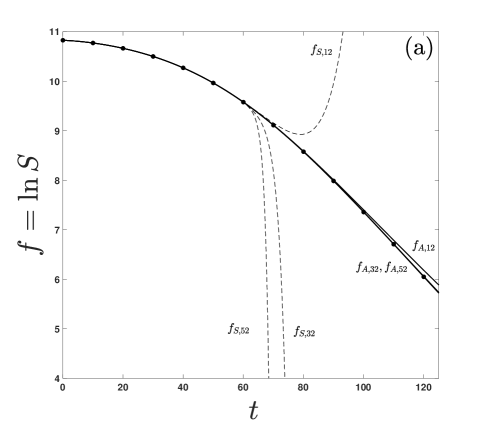
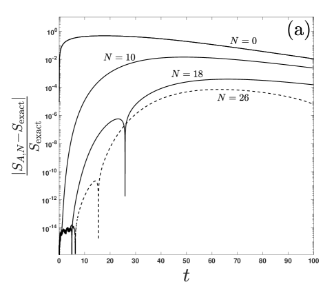
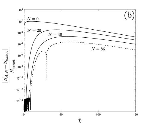
The SEIR approximant (15) is thus an analytic expression that, by construction, matches the correct behavior given by (14) and whose expansion about is exact to th-order. A comparison between the approximant solution (15) and the numerical solution to (1e) is provided in figures 1-4 with the relative error for all four cases provided in figure 5. The indicated error in figure 5 is calculated by comparing to its accurate numerical solution (assumed to be exact); curves showing the same order of accuracy are obtained when the other dependent variables of the model are examined.
|
|
|
|
 |
 |
 |
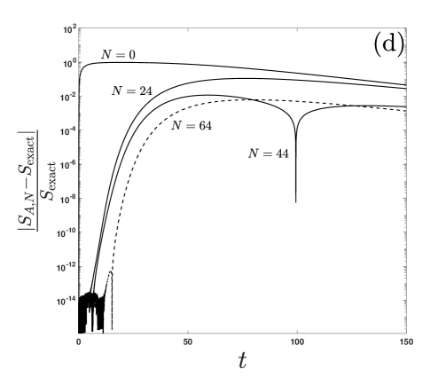 |
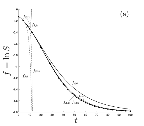
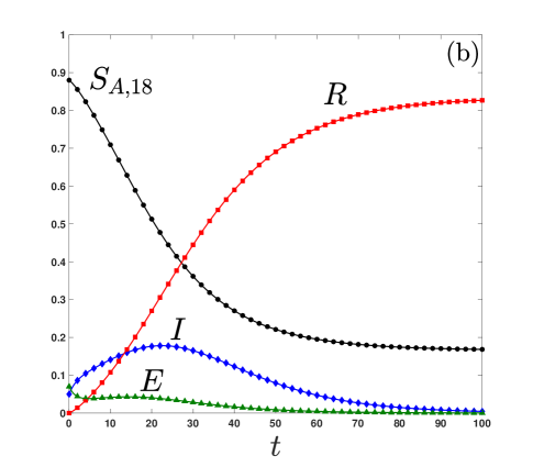
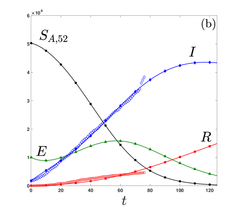
Figure 1a provides a typical comparison of the -term series solution (9d) denoted by (dashed lines), the -term approximant (15) denoted by (solid lines), and the numerical solution (’s). Note that the series solution has a finite radius of convergence as evidenced by the poor agreement and divergence from the numerical solution at larger times, even as additional terms are included. By contrast, the approximant converges as additional terms are included. For , the approximant is visibly indistinguishable from the numerical solution on the scale of figure 1a. Figure 5a provides the relative error of the approximant for the data shown in figure 1. Increasing the number of terms beyond does improve accuracy up to a point, but a minimum error barrier is eventually reached of (10-6) at ; note that, to make this assessment, we take the maximum relative error with respect to time for each (the maxima in figure 5a). For larger values of , the maximum error increases, and the approximant begins to diverge, i.e. there is an optimal value of at which to truncate the approximant. Asymptotic approximants can exhibit an optimal truncation Beachley et al. (2018); Belden et al. (2020) as is often observed with asymptotic expansions in general Bender and Orszag (1978). We emphasize here that a numerical solution is not needed to assess convergence of approximants to within their optimal truncation; convergence in the Cauchy sense (i.e., the distance between approximants decreases with increasing ) may be examined. In addition to this issue, deficient approximants are possible with increasing due to zeros that can arise in the denominator of (15). Such approximants are ignored in assessing convergence. To avoid this behavior, the lowest number of terms that yields the desired accuracy should be chosen. The convergence of the approximant with increasing (up until its optimal truncation) is a necessary condition for a valid approximant. In figure 1b, the converged () asymptotic approximant for is used to obtain analytic solutions for , , , and from (8d), which are compared with the numerical solution for these quantities. The approximant for agrees with numerics within the visible scale of the plot, with errors quantified by figure 5a.
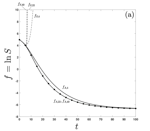
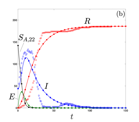
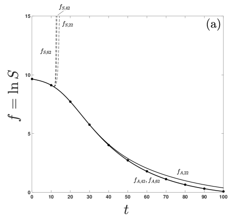
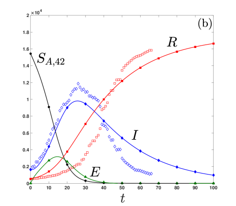
Figure 1 results described above correspond to a case examined in Rachah and Torres (2017) to model an Ebola outbreak. In figures 2, 3, and 4, the approximant is applied to COVID-19 data John Hopkins University CSSE for Yunan (China), Sweden, and Japan, respectively. Figure 5b-d provide the relative error for these cases; the largest indicated value of in each figure (corresponding to dashed curves) is the optimal truncation as discussed above for figure 5a. Note that we extensively surveyed the available COVID-19 data John Hopkins University CSSE , and the results in figures 2-5 are representative of the fits and variability in the number of terms needed for convergence of the approximant up to its optimal truncation.
Note that the reported COVID-19 outbreak data John Hopkins University CSSE is provided in terms of confirmed cases, recovered individuals, and deaths per day. We use recovered + deaths as an approximation to the removed population and use confirmed recovered deaths as an approximation to in the SEIR model. It is acknowledged that the actual COVID-19 data is influenced by effects not included in the SEIR model, and this can affect the ability of the model to closely fit actual COVID-19 data. The data approximations made here are to enable comparisons with model predictions. The ability of the approximant to match numerical results is unaffected by such approximations. Disagreement between the model and epidemic data after fitting is attributed to the applicability of the SEIR model and not the approximant.
In figures 2-4, a least squares fit to and data is used to extract SEIR parameters , , and initial conditions and . To do so, the initial values of and are taken directly from the COVID-19 data set John Hopkins University CSSE . Additionally, the time is chosen such that disease has progressed to a point where initial trends are observed, so that curve shapes are consistent with those reasonably predicted by the SEIR model. Adjustments such as this have been well described in fits done in previous work Peirlinck et al. (2020); Linka et al. (2020). The initial guesses for the iterative least-squares fit are taken from data fits for earlier times than examined here Peirlinck et al. (2020); Linka et al. (2020).
Our results demonstrate that an asymptotic approximant can be used to provide accurate analytic solutions to the SEIR model. Future work should examine the ability of the asymptotic approximant technique to yield closed-form solutions for even more sophisticated epidemic models, as well as their endemic counterparts Hethcote (2008).
References
- Barlow et al. (2012) N. S. Barlow, A. J. Schultz, S. J. Weinstein, and D. A. Kofke, J. Chem. Phys. 137, 204102 (2012).
- Barlow et al. (2014) N. S. Barlow, A. J. Schultz, S. J. Weinstein, and D. A. Kofke, AIChE J. 60, 3336 (2014).
- Barlow et al. (2015) N. S. Barlow, A. J. Schultz, S. J. Weinstein, and D. A. Kofke, J. Chem. Phys. 143, 071103:1 (2015).
- Barlow et al. (2017) N. S. Barlow, C. R. Stanton, N. Hill, S. J. Weinstein, and A. G. Cio, Q. J. Mech. Appl. Math. 70, 21 (2017).
- Barlow, Weinstein, and Faber (2017) N. S. Barlow, S. J. Weinstein, and J. A. Faber, Class. Quant. Grav. 34, 1 (2017).
- Beachley et al. (2018) R. J. Beachley, M. Mistysyn, J. A. Faber, S. J. Weinstein, and N. S. Barlow, Class. Quant. Grav. 35, 1 (2018).
- Belden et al. (2020) E. R. Belden, Z. A. Dickman, S. J. Weinstein, A. D. Archibee, E. Burroughs, and N. S. Barlow, Q. J. Mech. Appl. Math. 73, 36 (2020).
- Barlow and Weinstein (2020) N. S. Barlow and S. J. Weinstein, Physica D 408, 1 (2020).
- Baker Jr. and Gammel (1961) G. A. Baker Jr. and J. L. Gammel, J. Math. Anal. Appl. 2, 21 (1961).
- Bender and Orszag (1978) C. M. Bender and S. A. Orszag, Advanced Mathematical Methods for Scientists and Engineers I: Asymptotic Methods and Perturbation Theory (McGraw-Hill, 1978).
- Kermack and McKendrick (1927) W. O. Kermack and A. G. McKendrick, Proc. Roy. Soc. London A 115, 700 (1927).
- Hethcote (2008) H. W. Hethcote, in Mathematical Understanding of Infectious Disease Dynamics, edited by S. Ma and Y. Xia (World Scientific Publishing, 2008).
- Rachah and Torres (2017) A. Rachah and D. F. M. Torres, Math Method Appl. Sci. 40, 6155 (2017).
- (14) “https://github.com/chebfun/chebfun/blob/master/padeapprox.m,” .
- Gonnet, Güttel, and Trefethen (2013) P. Gonnet, S. Güttel, and L. N. Trefethen, SIAM Rev. 55, 101 (2013).
- (16) https://www.mathworks.com/matlabcentral/fileexchange/77007-approximantcoefficientsseir.
- (17) John Hopkins University CSSE, “Novel coronavirus (covid-19) cases,” https://github.com/CSSEGISandData/COVID-19.
- Peirlinck et al. (2020) M. Peirlinck, K. Linka, F. S. Costabal, and E. Kuhl, Biomech. Model. Mechan. doi.org/10.1007/s10237-020-01332-5, 1 (2020).
- Linka et al. (2020) K. Linka, M. Peirlinck, F. S. Costabal, and E. Kuhl, Comput. Method Biomec. doi.org/10.1080/10255842.2020.1759560, 1 (2020).