Discriminative reconstruction via simultaneous dense and sparse coding

Abstract

Discriminative features extracted from the sparse coding model have been shown to perform well for classification. Recent deep learning architectures have further improved reconstruction in inverse problems by considering new dense priors learned from data. We propose a novel dense and sparse coding model that integrates both representation capability and discriminative features. The model studies the problem of recovering a dense vector $\bm{x}$ and a sparse vector $\bm{u}$ given measurements of the form $\bm{y}=\bm{A}\bm{x}+\bm{B}\bm{u}$. Our first analysis proposes a geometric condition based on the minimal angle between spanning subspaces corresponding to the matrices $\bm{A}$ and $\bm{B}$ that guarantees unique solution to the model. The second analysis shows that, under mild assumptions, a convex program recovers the dense and sparse components. We validate the effectiveness of the model on simulated data and propose a dense and sparse autoencoder (DenSaE) tailored to learning the dictionaries from the dense and sparse model. We demonstrate that (i) DenSaE denoises natural images better than architectures derived from the sparse coding model ($\bm{B}\bm{u}$), (ii) in the presence of noise, training the biases in the latter amounts to implicitly learning the $\bm{A}\bm{x}+\bm{B}\bm{u}$ model, (iii) $\bm{A}$ and $\bm{B}$ capture low- and high-frequency contents, respectively, and (iv) compared to the sparse coding model, DenSaE offers a balance between discriminative power and representation.

1 Introduction

The problem of representing data as a linear mixture of components finds applications in many areas of signal and image processing [7, 38]. Variational partial differential equations (PDE) approaches in [4, 62] develop an image decomposition model whereby a target image is decomposed into a piecewise smooth component (cartoon) and a periodic component (texture). Another approach is based on the idea that a desirable model would have multiple matrices each capturing different structures of the image e.g. $\bm{\Phi}_{1}$ is a matrix modeling texture and $\bm{\Phi}_{2}$ is a matrix modeling cartoon. Along these methods is Morpohological Component Analysis (MCA) [25] which utilizes pre-specified dictionaries and a a sparsity prior on the representation coefficients. In the simplest setting, an image $\bm{y}$ is modeled in MCA as $\bm{y}\approx\sum_{k=1}^{2}\bm{\Phi}_{k}\bm{x}_{k}$ where $\bm{\Phi}_{1},\bm{\Phi}_{2}$ are the pre-specified structured dictionaries capturing different morphologies of the image. The MCA model is then based on the idea that the sparsest representation of each component is attained in the pre-set dictionary component. In contrast to MCA which imposes sparsity for all mixture coefficients, the proposed model in this paper adopts a combination of smooth and sparse regularization.

Related motivating problems for representing data as a linear mixture are the background/foreground separation problem [67] and anomaly detection in images [16]. In the former problem, a widely used approach is the robust principal component analysis (RPCA) algorithm [15] which is based on decomposing a data matrix into low rank (background) and sparse (foreground) components. The latter problem, anomaly detection with images, arises in most manufacturing processes and methods based on decomposing the images into smooth and sparse components have been studied [64, 50]; however, no theoretical analysis has been conducted for that decomposition. In addition, in image anomaly detection the sparse and smooth components are localized, inhibiting the generality of the model.

In this paper, we study a model which decomposes a signal or image in consideration into a smooth part, sparse part, and noise. The prototypical form of our model is $\bm{y}=\bm{A}\bm{x}+\bm{B}\bm{u}+\bm{e}$ where $\bm{y}\in^{m}$ is the measured signal, $\bm{A}\bm{x}$ is the smooth component, $\bm{B}\bm{u}$ is the sparse component and $\bm{e}$ is noise. The smooth component is generated from the dictionary $\bm{A}\in^{m\times p}$ using a smooth coefficient $\bm{x}$. In turn, the sparse component is generated from the dictionary $\bm{B}\in^{m\times n}$ using a sparse vector $\bm{u}$. We use Tikhonov regularization [57] and $\ell_{1}$ regularization to promote smoothness and sparsity, respectively. With that, the general non-noisy problem we study in this paper is

$$\underset{\bm{x}\in^{p},\bm{u}\in^{n}}{\min}\quad||\bm{G}\bm{x}||_{2}^{2}+||\bm{u}||_{1}\quad\text{s.t.}\quad\bm{y}=\bm{A}\bm{x}+\bm{B}\bm{u},$$ (1.1)

where $\bm{G}$ is the Tikhonov regularization operator. Here on, we refer to the model in (1.1) as the dense and sparse coding problem. The word dense here refers to the smooth part and is used to emphasize that we do not require any sparsity.

Both MCA and the dense and sparse coding problem naturally lend themselves to and share a common theme with sparse coding and dictionary learning. Sparsity regularized deep neural network architectures have been used for image denoising and discriminative tasks such as image classification [51, 58, 49]. Recent work has highlighted some limitations of convolutional sparse coding (CSC) autoencoders and its multi-layer and deep generalizations  [56, 65] for data reconstruction. The work in [51] argues that the sparsity levels that CSC allows can only accommodate very sparse vectors, making it unsuitable to capture all features of signals such as natural images, and propose to compute the minimum mean-squared error solution under the CSC model, which is a dense vector capturing a richer set of features. Moreover, the majority of CSC frameworks subtract low-frequency components of images prior to applying convolutionl dictionary learning (CDL) for representation purposes [29]; however, this is not desired for denoising tasks where noise corrupts low frequencies in addition to the high spectrum. The goals of the paper are twofold. First, it presents a theoretical analysis of the dense and sparse coding problem. Second, we argue the dense representation $\bm{x}$ in a dictionary $\bm{A}$ is useful for reconstruction and the sparse representation $\bm{u}$ has discriminative capability.

1.1 Organization of paper

Section 2 discusses related work. In Section 3, we give some technical background to the main analysis. Section 4 presents the theoretical analysis of the paper. Phase transition, classification, and denoising experiments appear in Section 5. We conclude in Section 6. We start by defining notations.

1.2 Notation

Lowercase and uppercase boldface letters denote column vectors and matrices, respectively. Given a vector $\bm{x}\in^{n}$ and a support set $S\subset\{1,...,n\}$, $\bm{x}_{S}$ denotes the restriction of $\bm{x}$ to indices in $S$. $\text{supp}(\bm{x})$ denotes the support of a vector i.e. $\text{supp}(\bm{x})=\{i:x_{i}\neq 0\}$. For a matrix $\bm{A}\in^{m\times p}$, $\bm{A}_{S}$ is a submatrix of size $m\times|S|$ with column indices in $S$. The column space of a matrix $\bm{A}$ is designated by $\operatorname{Col}(\bm{A})$, its null space by $\text{Ker}(\bm{A})$. We denote the Euclidean, $\ell_{0}$, $\ell_{1}$, and $\ell_{\infty}$ norms of a vector $\bm{x}$, respectively as $||\bm{x}||_{2}$, $||\bm{x}||_{0}$, $||\bm{x}||_{1}$, and $||\bm{x}||_{\infty}$. The operator and infinity norm of a matrix $\bm{A}$ are respectively denoted as $\left|\left|\bm{A}\right|\right|$ and $\left|\left|\bm{A}\right|\right|_{\infty}$. The sign function, applied componentwise to a vector $\bm{x}$, is denoted by $\operatorname{sgn}(\bm{x})$. The indicator function is denoted by $\mathbbm{1}$. The column vector $\bm{e}_{i}$ denotes the vector of zeros except a $1$ at the $i$-th location. The orthogonal complement of a subspace $\bm{W}$ denoted by $\bm{W}^{\perp}$. The operator $\mathcal{P}_{\bm{W}}$ denotes the orthogonal projection operator onto the subspace $\bm{W}$. $\log(x)$ denotes the logarithm of $x$ in base $e$.

2 Related work

2.1 Compressive sensing from union of dictionaries

The dense and sparse coding problem is similar in flavor to sparse recovery in the union of dictionaries [22, 21, 24, 20, 33]. Most results in this literature take the form of an uncertainty principle that relates the sum of the sparsity of $\bm{x}$ and $\bm{u}$ to the mutual coherence between $\bm{A}$ and $\bm{B}$, and which guarantees that the representation is unique and identifiable by $\ell_{1}$ minimization. In [22], the authors study the problem of recovering $\bm{x}$ and $\bm{u}$ from $\bm{y}=\bm{A}\bm{x}+\bm{B}\bm{u}$ where $\bm{A}\in^{m\times m}$ is a discrete Fourier matrix (DFT) and $\bm{B}\in^{m\times m}$ is the identity matrix. Therein, under the assumption that the support of $\bm{u}$ is known, the result shows that $\bm{x}$ can be exactly recovered if $2||\bm{x}||_{0}||\bm{u}||_{0}<m$. This result for the Fourier-identity pair was further generalized to the case where $\bm{A}$ and $\bm{B}$ are orthonormal bases [24] and when the measurements come from a union of non-orthogonal bases [20, 33]. We remark that all the aforementioned results assume sparsity on both $\bm{x}$ and $\bm{u}$.

2.2 Error correction

The problem of recovering a signal $\bm{x}$ given the measurement model $\bm{y}=\bm{A}\bm{x}+\bm{u}$ where $\bm{u}$ is a sparse error vector is the sparse error correction problem [10]. The work therein considers a tall measurement matrix $\bm{A}$ and assumes that the fraction of corrupted entries is suitably bounded. To obtain a sparse minimization program, the matrix $\bm{A}$ is eliminated by a matrix $\bm{B}$, where $\bm{B}\bm{A}=0$, resulting $\bm{B}\bm{y}=\bm{B}\bm{u}$. The resulting model is then solved via $\ell_{1}$ minimization and exactness is shown under the restricted isometry condition on $\bm{B}$. The works in [63, 43, 48, 55, 54] study the general error correction problem $\bm{y}=\bm{A}\bm{x}+\bm{B}\bm{u}$ under different models of the signal $\bm{x}$, the sparse interference vector $\bm{u}$ and under different assumptions on the measurement matrices $\bm{A}$ and $\bm{B}$. We note that all the aforementioned works consider a single sparsifying norm to recover the components $\bm{x}$ and $\bm{u}$. In contrast, we use mixed norms that impose the Tikhonov and sparsity regularization. We also note that when $\bm{A}$ is fat, the setting we consider in this paper, our problem departs from the sparse error correction problem.

2.3 Weighted Lasso

When there is some prior on the support of the underlying sparse vector $\bm{y}$ given measurements of the form $\bm{y}=\bm{B}\bm{u}$, the works in [36, 39, 61, 45, 28, 27] consider a weighted Lasso program. Assume that the estimate of the support of $\bm{u}$ is $T\subset\{1,...,n\}$. The standard weighted Lasso considers the following optimization program

$$\underset{u}{\min}\quad||\bm{u}||_{1,w}\quad\text{subject to}\quad\bm{y}=\bm{B}\bm{u},$$

where $||\bm{u}||_{1,\bm{w}}=\sum_{i=1}^{n}w_{i}u_{i}$ and $\bm{w}\in^{n}$ indicates the vector of weights. For instance, Mansour and Saab [39] set the weights as follows: $w_{i}\in[0,1]$ if $i\in T$ and $1$ otherwise. The aforementioned works discuss the recovery of the underlying signal using weighted Lasso under some conditions on the weights, size and accuracy of the estimated support. One approach for the feasibility constraint in (1.1) is to reformulate it as a weighted Lasso problem in a combined dictionary $[\bm{A}\,\,\bm{B}]$ where the support estimate is the support of $\bm{x}$. This formulation has few limitations. First, the recovery guarantees in weighted Lasso require accuracy of the estimated support which would depend on the number of columns of $\bm{A}$. Second, these guarantees impose uniform structure on the combined dictionary e.g. weighted null space conditions while our conditions allow deterministic dictionary $\bm{A}$ and random dictionary $\bm{B}$. Finally, even in the regime where weighted Lasso might succeed in recovering the underlying $\bm{x}$ and $\bm{u}$, it does not guarantee that $\bm{A}\bm{x}$ is smooth as that regularization is not reflected in the Lasso optimization.

2.4 Morphological component analysis (MCA)

Morphological Component Analysis (MCA) considers the decomposition of a signal or image into different components with each component having a specific structure (morphology) [52, 53, 9, 25]. In MCA, the specific structure is imposed via sparsity with respect to pre-specified dictionaries. Specifically, given $K$ dictionaries $\{\bm{\Phi}_{1},...,\bm{\Phi}_{K}\}$, we model the data $\bm{y}$ as a superposition of $K$ linear components as follows: $\bm{y}=\sum_{i=1}^{K}\bm{\Phi}_{i}\bm{y}_{i}$ where $\bm{y}_{i}$ is assumed to be sparse in $\bm{\Phi}_{i}$ but it is not as sparse (or not sparse at all) in other dictionaries. With this set up, the dictionaries discriminate between the different components. In [52] a basis pursuit approach to solve the MCA is employed and its utility is illustrated in several examples e.g. separating texture from the smooth part of an image. The main difference of our model from MCA is a smooth-sparse decomposition as opposed to sparse-sparse decomposition with pre-set dictionaries that contain information about targeted morphologies. The theory and analysis of the two models is also markedly different as we consider a smoothness regularizer.

2.5 Dictionary learning and unrolling

Given a data set, learning a dictionary in which each example admits a sparse representation is useful in a number of tasks [3, 37]. This problem, known as sparse coding [44] or dictionary learning [2, 29], has been the subject of investigation in recent years in the signal processing community. A growing body of work, referred to as algorithm unrolling [42], has mapped the sparse coding problem into encoders for sparse recovery [30]. In this paper, we unroll the dense and sparse coding problem for a principled design of an autoencoder. The appeal of the autoencoder is that it learns dense representation $\bm{x}$ in a dictionary $\bm{A}$ useful for reconstruction and sparse representation $\bm{u}$ which has discriminative capability.

2.6 Contribution

We focus on (1.1) and start by first providing theoretical guarantees for the feasibility problem $\bm{y}=\bm{A}\bm{x}+\bm{B}\bm{u}$. Our first result is based on a geometric condition on the minimum principal angle between certain subspaces. Next, we prove that the convex program in (1.1) recovers the underlying components $\bm{x}$ and $\bm{u}$ under some mild assumptions on the measurement matrices and the Tikhonov regularizer. We empirically validate the effectiveness of our methods through phase transition curves and make a direct comparison to noisy compressive sensing, highlighting the latter’s inability to recover signals adhering to our proposed model. We then apply our optimization algorithm to sense real data and validate the expected properties of the sparse and smooth components.

We connect the proposed model to dictionary learning/algorithm unrolling by proposing a dense and sparse autoencoder (DenSaE). We demonstrate the superior discriminative and representation capabilities of DenSaE compared to sparse coding networks in the task of reconstruction and classifying MNIST dataset. In this task, we characterize the role of dense and sparse learned components; we argue that the dense representation $\bm{x}$ is useful for reconstruction and the sparse representation $\bm{u}$ has discriminative capability. Moreover, in an image denoising task, we show the outpefromance of DenSaE against networks strictly performing sparse coding.

3 Technical background

In this section, we start by briefly reviewing uniqueness results for compressive sensing with exact measurements. The typical assumption in these analysis is to assume the measurement matrices satisfy certain conditions such as the restricted isometry property (RIP) and coherence. In our setting, we employ RIPless recovery analysis [12, 32] which will be referred to and used in our the proof of Theorem 7. We note that existing anisotropic analysis is based on a single measurement matrix. For our model, the anisotropic analysis is applied to a certain matrix derived from $\bm{A}$, $\bm{B}$ and the Tikhonov regularizer $\bm{G}$.

3.1 Compressive sensing with exact measurements

An underdetermined linear system $\bm{y}=\bm{B}\bm{u}$ where $\bm{y}\in^{m}$ and $\bm{B}\in^{m\times n}$ with $n>m$ generally has infinitely many solutions. One prior for the recovery of the solution is sparsity of the underlying vector $\bm{u}$. This leads to the following optimization problem

$$\underset{\bm{u}\in^{m}}{\min}\quad\left|\left|\bm{u}\right|\right|_{0}\quad\text{s.t.}\quad\bm{y}=\bm{A}\bm{u}.$$ (3.1)

While (3.1) is a natural program, it is known to be computationally intractable. Common alternatives are basis pursuit (BP) [59, 18] and iterative greedy methods such as orthogonal matching pursuit (OMP)[19, 46, 60]. In basis pursuit, (3.1) is modified by considering a convex relaxation of the $\ell_{0}$ norm leading to the $\ell_{1}$ minimization problem.

$$\underset{\bm{u}\in^{m}}{\min}\quad\left|\left|\bm{u}\right|\right|_{1}\quad\text{s.t.}\quad\bm{y}=\bm{B}\bm{u}.$$ (3.2)

A fundamental question is under what conditions they identify the underlying solution for (3.1). A related part of this question is when the $\ell_{0}$ minimization problem admits a unique solution. One condition is the restricted isometry property (RIP) [13]. The $s$-restricted isometry constant of an $m\times n$ measurement matrix $B$ is the smallest constant $\delta_{s}$ such that

$$(1-\delta_{s})||\bm{u}||^{2}\leq||\bm{B}\bm{u}\|^{2}\leq(1+\delta_{s})||\bm{u}||^{2},$$

holds for all $s$-sparse signals $\bm{u}$ (an $s$-sparse vector has at most $s$ non-zero entries). Small RIP constants ensure unique solution of the $\ell_{0}$ minimization problem and further provide the guarantee that the $\ell_{1}$ relaxation in (3.2) is exact [11]. It is known that random measurement matrices have small RIP constants [14, 5]. Another condition for analysis is based on the coherence of a measurement matrix $\bm{B}$ defined as

$$\mu=\underset{i\neq j}{\max}\,\,|\bm{b}_{i}^{T}\bm{b}_{j}|,$$

where $\bm{b}_{i}$ denotes the $i$-th column of $\bm{B}$ which is assumed to be unit-norm. To state the next result, consider $\bm{y}=\bm{B}\bm{u}^{*}$ where $\bm{u}^{*}$ is the underlying sparse vector. If $\left|\left|\bm{u}^{*}\right|\right|_{0}<\frac{1}{2}\left(1+\frac{1}{\mu}\right)$, the $\ell_{0}$ problem admits a unique solution and both BP and OMP relaxations are exact [20, 31, 59].

3.2 Compressive sensing with structured random matrices

We review the technical results in [12, 32] which consider conditions for the exact recovery of the $\ell_{1}$ minimization problem for the setting of structured measurement matrices. In this setting, we do not assume restricted isometry property (RIP) of the measurement matrices [13] and this broadens the sensing matrices that can be employed. We consider a sequence of i.i.d random vectors $\bm{b}_{1},...,\bm{b}_{m}$ drawn from some distribution $F$ on ⁿ and with measurements defined as $\bm{y}_{i}=\bm{b}_{i}^{T}\bm{u}^{*}$. Two properties are essential to the analysis. The first is the isotropy property which states that $E[\bm{b}\bm{b}^{T}]=\bm{I}$ for $\bm{b}\sim F$. The second property is the incoherence property. The incoherence parameter is the smallest number $\mu(F)$ such that

$$\underset{1\leq i\leq n}{\max}\,|\langle\bm{b},\bm{e}_{i}\rangle|^{2}\leq\mu(F),$$ (3.3)

holds almost surely. Given these assumptions, the work in [12] provides the following theoretical result.

Theorem 1 ([12]).

Let $\bm{B}=\frac{1}{\sqrt{m}}\sum_{i=1}^{m}\bm{b}_{i}\bm{e}_{i}^{T}$ be a measurement matrix and let $\bm{u}$ be a fixed but otherwise arbitrary $s$-sparse vector in ⁿ. Then with probability at least $1-\frac{5}{n}-e^{-\beta}$ , $\bm{u}$ is the unique minimizer to

$$\underset{\bm{u}}{\min}\quad||\bm{u}||_{1}\quad\text{subject to}\quad\bm{y}=\bm{B}\bm{u},$$

provided that $m\geq C_{\beta}\mu(F)s\log n$. The constant $C_{\beta}=C_{0}(1+\beta)$ where $C_{0}$ is some constant.

We note that the definition of $\bm{B}$ based on re-scaling the vectors $\bm{b}_{1},\bm{b}_{2},...,\bm{b}_{m}$ is done so that the columns of $\bm{B}$ are approximately unit-normed. The work in [32] extends the above result without assuming the isotropy property. Let $\bm{\Sigma}=E[\bm{b}\bm{b}^{T}]^{\frac{1}{2}}$, where as before $\bm{b}$ is drawn from distribution $F$ on ⁿ, denote the covariance matrix. The anisotropic analysis in [32] is based on two properties pertaining to the measurement matrix. The first is the incoherence property which is formally defined as follows. The incoherence parameter is the smallest number $\mu(F)$ such that

$$\underset{1\leq i\leq n}{\max}\,|\langle\bm{b}\,,\bm{e}_{i}\rangle|^{2}\leq\mu(F)\,\,\text{ and }\,\,\underset{1\leq i\leq n}{\max}\,|\langle\bm{b}\,,E[\bm{b}\bm{b}^{*}]^{-1}\bm{e}_{i}\rangle|^{2}\leq\mu(F)$$ (3.4)

hold almost surely. The second property is based on the conditioning of the covariance matrix. More precisely, it is based on an $s$-sparse condition number which we restate the definition in [32] below.

Definition 1.

[32] The largest and smallest $s$-sparse eigenvalue of a matrix $\bm{X}$ are given by $\lambda_{\max}(s,\bm{X}):=\underset{||\bm{v}||_{0}\leq s}{\max}\,\frac{||\bm{X}\bm{v}||_{2}}{||\bm{v}||_{2}}$ and $\lambda_{\min}(s,\bm{X}):=\underset{||\bm{v}||_{0}\leq s}{\min}\,\frac{||\bm{X}\bm{v}||_{2}}{||\bm{v}||_{2}}.$ The $s$-sparse condition number of $\bm{X}$ is $\displaystyle\text{cond}(s,\bm{X})=\frac{\lambda_{\max}(s,\bm{X})}{\lambda_{\min}(s,\bm{X})}$.

Given these assumptions, the main result in [32] is stated below.

Theorem 2.

[32] Let $\bm{B}=\frac{1}{\sqrt{m}}\sum_{i=1}^{m}\bm{b}_{i}\bm{e}_{i}^{T}$ be a measurement matrix and let $\bm{u}$ be a fixed but otherwise arbitrary $s$-sparse vector in ⁿ. Define $\kappa_{s}=\max\{\text{cond}(s,\bm{\Sigma}),\text{cond}(s,\bm{\Sigma}^{-1})\}$ and let $\beta\geq 1$. If the number of measurements fulfills $m\geq C\kappa_{s}\,\mu(F)\,\beta\,s\log n$, then the solution $\bm{u}$ of the convex program $\underset{\bm{u}}{\min}\,\,\,||\bm{u}||_{1}\,\,\text{subject to}\,\,\,\bm{y}=\bm{B}\bm{u},$ is unique and equal to $\bm{u}^{*}$ with probability at least $1-e^{-\beta}$.

The proof of Theorem 1 and Theorem 2 is based on the dual certificate approach. The idea is to first propose a dual certificate vector $\bm{v}$ with sufficient conditions that ensure uniqueness of the minimization problem. It then remains to construct the dual certificate satisfying the conditions. For later reference, we note that the works in [12, 32] construct a dual certificate $\bm{v}$ satisfying the following conditions

$$||\bm{v}_{S}-\operatorname{sgn}(\bm{u}^{*}_{S})||_{2}\leq\tfrac{1}{4}\,\,\,\,\text{and}\,\,\,\,||\bm{v}_{S^{\perp}}||_{\infty}\leq\tfrac{1}{4}.$$ (3.5)

The following condition follows from the assumptions in Theorem 1 and 2

$$||\bm{\Delta}_{S}||_{2}\leq 2||\bm{\Delta}_{S^{\perp}}||_{2},\quad\text{for}\quad\bm{\Delta}\in\text{Ker}(\bm{B}).$$ (3.6)

4 Theoretical Analysis

The dense and sparse coding problem studies the solutions of the linear system $\bm{y}=\bm{A}\bm{x}+\bm{B}\bm{u}$. Given matrices $\bm{A}\in^{m\times p}$ and $\bm{B}\in^{m\times n}$ and a vector $\bm{y}\in^{m}$, the goal is to provide conditions under which there is a unique solution ($\bm{x}^{*},\bm{u}^{*}$), where $\bm{u}^{*}$ is $s$-sparse, and an algorithm for recovering it.

4.1 Feasibility problem

In this subsection, we first study the uniqueness of solutions to the linear system accounting for the different structures the measurement matrices $\bm{A}$ and $\bm{B}$ can have. A uniqueness result can be readily obtained by assuming orthogonality of $\operatorname{Col}(\bm{A})$ and $\operatorname{Col}(\bm{B})$. In what follows, we establish uniqueness results for the general setting. The main result of this subsection is Theorem 4 which, under a natural geometric condition based on the minimum principal angle between the column space of $\bm{A}$ and the span of $s$ columns in $\bm{B}$, establishes a uniqueness result for the dense and sparse coding problem. Since the vector $\bm{u}$ in the proposed model is sparse, we consider the classical setting of an overcomplete measurement matrix $\bm{B}$ with $n\gg m$. The next theorem provides a uniqueness result assuming a certain direct sum representation of the space ^m. We first note that, for $\bm{A}\in^{m\times p}$ with $p\gg m$, any $\bm{z}\in\operatorname{Ker}(\bm{A})$ can be added to any solution $\bm{x}$. With that, we consider uniqueness modulo the vectors in $\operatorname{Ker}(\bm{A})$ i.e. any feasible solution is assumed to be in $\operatorname{Ker}(\bm{A})^{\perp}$.

Theorem 3.

Assume that there exists at least one solution to $\bm{y}=\bm{A}\bm{x}+\bm{B}\bm{u}$, namely the pair $(\bm{x}^{*},\bm{u}^{*})$. Let $S$, with $|S|=s$, denote the support of $\bm{u}^{*}$. If $\bm{B}_{S}$ has full column rank and ${}^{m}=\operatorname{Col}(\bm{A})\oplus\operatorname{Col}(\bm{B}_{S})$, the only unique solution to the linear system, with the condition that any feasible $s$-sparse vector $\bm{u}$ is supported on $S$ and any feasible $\bm{x}$ is in $\operatorname{Ker}(\bm{A})^{\perp}$, is $(\bm{x}^{*},\bm{u}^{*})$.

Proof.

Let $(\bm{x},\bm{u})$, with $\bm{u}$ supported on $S$ and $\bm{x}\in\operatorname{Ker}(\bm{A})^{\perp}$, be another solution pair. It follows that $\bm{A}\bm{\delta_{1}}+\bm{B}_{S}(\bm{\delta_{2}})_{S}=\bm{0}$ where $\bm{\delta_{1}}=\bm{x}-\bm{x}^{*}$ and $\bm{\delta_{2}}=\bm{u}-\bm{u}^{*}$. Let $\bm{U}\in^{m\times r}$ and $\bm{V}\in^{m\times q}$ be matrices whose columns are the orthonormal bases of $\operatorname{Col}(\bm{A})$ and $\operatorname{Col}(\bm{B}_{S})$, respectively. The equation $\bm{A}\bm{\delta_{1}}+\bm{B}_{S}(\bm{\delta_{2}})_{S}=\bm{0}$ can equivalently be written as $\sum_{i=1}^{r}\langle\bm{A}\bm{\delta_{1}}\,,\bm{U}_{i}\rangle\bm{U}_{i}+\sum_{i=1}^{q}\langle\bm{B}_{S}(\bm{\delta_{2}})_{S}\,,\bm{V}_{i}\rangle\bm{V}_{i}=\bm{0}$ with $\bm{U}_{i}$ and $\bm{V}_{i}$ denoting the $i$-th columns of $\bm{U}$ and $\bm{V}$, respectively. More compactly, we have $\begin{bmatrix}\bm{U}&\bm{V}\end{bmatrix}\begin{bmatrix}\{\langle\bm{A}\bm{\delta_{1}}\,,\bm{U}_{i}\rangle\}_{i=1}^{r}\\ \{\langle\bm{B}_{S}(\bm{\delta_{2}})_{S}\,,\bm{V}_{i}\rangle\}_{i=1}^{q}\end{bmatrix}=\bm{0}$. Noting that the matrix $\begin{bmatrix}\bm{U}&\bm{V}\end{bmatrix}$ has full column rank, the homogeneous problem admits the trivial solution implying that $\bm{A}\bm{\delta_{1}}=\bm{0}$ and $\bm{B}_{S}(\bm{\delta_{2}})_{S}=\bm{0}$. Since $\bm{B}_{S}$ has full column rank and $\bm{\delta_{1}}\in\{\operatorname{Ker}(\bm{A})\cap\operatorname{Ker}(\bm{A})^{\perp}\}$, it folows that $\bm{\delta_{1}}=\bm{\delta_{2}}=\bm{0}$. Therefore, $(\bm{x}^{*},\bm{u}^{*})$ is the unique solution. ∎

The uniqueness result in the above theorem hinges on the representation of the space ^m as the direct sum of the subspaces $\operatorname{Col}(\bm{A})$ and $\operatorname{Col}(\bm{B}_{S})$. We use the definition of the minimal principal angle between two subspaces, and its formulation in terms of singular values [8], to derive an explicit geometric condition for the uniqueness analysis of the linear system in the general case.

Definition 2.

Let $\bm{U}\in^{m\times r}$ and $\bm{V}\in^{m\times q}$ be matrices whose columns are the orthonormal basis of $\operatorname{Col}(\bm{A})$ and $\operatorname{Col}(\bm{B})$, respectively. The minimum principal angle between the subspaces $\operatorname{Col}(\bm{A})$ and $\operatorname{Col}(\bm{B})$ is defined as follows

$$\cos(\mu(\bm{U},\bm{V}))=\underset{\bm{u}\in\operatorname{Col}(\bm{U}),\bm{v}\in\operatorname{Col}(\bm{V})}{\max}\,\,\frac{\bm{u}^{T}\bm{v}}{||\bm{u}||_{2}||\bm{v}||_{2}},$$ (4.1)

In addition, $\cos(\mu(\bm{U},\bm{V}))=\sigma_{1}(\bm{U}^{T}\bm{V})$ where $\sigma_{1}$ denotes the largest singular value.

Theorem 4.

Assume that there exists at least one solution to $\bm{y}=\bm{A}\bm{x}+\bm{B}\bm{u}$, namely the pair $(\bm{x}^{*},\bm{u}^{*})$. Let $S$, with $|S|=s$, denote the support of $\bm{u}^{*}$. Assume that $\bm{B}_{S}$ has full column rank . Let $\bm{U}\in^{m\times r}$ and $\bm{V}\in^{m\times q}$ be matrices whose columns are the orthonormal bases of $\operatorname{Col}(\bm{A})$ and $\operatorname{Col}(\bm{B}_{S})$, respectively. If $\cos(\mu(\bm{U},\bm{V}))=\sigma_{1}(\bm{U}^{T}\bm{V})<1$, the only unique solution to the linear system, with the condition that any feasible $s$-sparse vector $\bm{u}$ is supported on $S$ and any feasible $\bm{x}$ is in $\operatorname{Ker}(\bm{A})^{\perp}$, is $(\bm{x}^{*},\bm{u}^{*})$.

Proof.

Consider any candidate solution pair $(\bm{x}^{*}+\bm{\delta_{1}},\bm{u}^{*}+\bm{\delta_{2}})$ with $\bm{\delta_{2}}$ supported in S. We will prove uniqueness by showing that $\bm{A}\bm{\delta_{1}}+\bm{B}_{S}(\bm{\delta_{2}})_{S}=0$ if and only if $\bm{\delta_{1}}=\bm{0}$ and $\bm{\delta_{2}}=\bm{0}$. Using the orthonormal basis set $\bm{U}$ and $\bm{V}$, $\bm{A}\bm{\delta_{1}}+\bm{B}_{S}(\bm{\delta_{2}})_{S}$ can be represented as : $\bm{A}\bm{\delta_{1}}+\bm{B}_{S}(\bm{\delta_{2}})_{S}=\begin{bmatrix}\bm{U}&\bm{V}\\ \end{bmatrix}\begin{bmatrix}\bm{U}^{T}\bm{A}\bm{\delta_{1}}\\ \bm{V}^{T}\bm{B}_{S}(\bm{\delta_{2}})_{S}\\ \end{bmatrix}$. For simplicity of notation, let $\bm{K}$ denote the block matrix: $\displaystyle\bm{K}=\begin{bmatrix}\bm{U}&\bm{V}\\ \end{bmatrix}$. If we can show that the columns of $\bm{K}$ are linearly independent, it follows that $\bm{A}\bm{\delta_{1}}+\bm{B}_{S}(\bm{\delta_{2}})_{S}=\bm{0}$ if and only if $\bm{A}\bm{\delta_{1}}=\bm{0}$ and $\bm{B}_{S}(\bm{\delta_{2}})_{S}=\bm{0}$. We now consider the matrix $\bm{K}^{T}\bm{K}$ which has the following representation

$$\bm{K}^{T}\bm{K} =\begin{bmatrix}[\bm{I}]_{r\times r}&[\bm{U}^{T}\bm{V}]_{r\times q}\\ [\bm{V}^{T}\bm{U}]_{q\times r}&[\bm{I}]_{q\times q}\end{bmatrix}$$

$$=\begin{bmatrix}[\bm{I}]_{r\times r}&[\bm{0}]_{r\times q}\\ [\bm{0}]_{q\times r}&[\bm{I}]_{q\times q}\end{bmatrix}+\begin{bmatrix}[\bm{0}]_{r\times r}&[\bm{U}^{T}\bm{V}]_{r\times q}\\ [\bm{V}^{T}\bm{U}]_{q\times r}&[\bm{0}]_{q\times q}\end{bmatrix}.$$

With the singular value decomposition of $\bm{U}^{T}\bm{V}$ being $\bm{U}^{T}\bm{V}=\bm{Q}\mathbf{\bm{\Sigma}}\bm{R}^{T}$, the last matrix in the above representation has the following equivalent form $\begin{bmatrix}\bm{0}&\bm{U}^{T}\bm{V}\\ \bm{V}^{T}\bm{U}&\bm{0}\end{bmatrix}=\begin{bmatrix}\bm{Q}&\bm{0}\\ \bm{0}&\bm{R}\end{bmatrix}\begin{bmatrix}\bm{0}&\bm{\Sigma}\\ \bm{\Sigma}&\bm{0}\end{bmatrix}\begin{bmatrix}\bm{Q}&\bm{0}\\ \bm{0}&\bm{R}\end{bmatrix}^{T}$. It now follows that $\begin{bmatrix}\bm{0}&\bm{U}^{T}\bm{V}\\ \bm{V}^{T}\bm{U}&\bm{0}\end{bmatrix}$ is similar to the matrix $\begin{bmatrix}\bm{0}&\mathbf{\bm{\Sigma}}\\ \mathbf{\bm{\Sigma}}&\bm{0}\end{bmatrix}$. Hence, the nonzero eigenvalues of $\bm{K}^{T}\bm{K}$ are $1\pm\sigma_{i}$, $1\leq i\leq\min(p,q)$, with $\sigma_{i}$ denoting the $i$-th largest singular value of $\bm{U}^{T}\bm{V}$. Using the assumption $\sigma_{1}<1$ results the bound $\lambda_{\min}\left(\bm{K}^{T}\bm{K}\right)>0$. It follows that the columns of $\bm{K}$ are linearly independent, and hence $\bm{A}\bm{\delta_{1}}=\bm{0}$ and $\bm{B}_{S}(\bm{\delta_{2}})_{S}=\bm{0}$. Since $\bm{B}_{S}$ is full column rank and $\bm{\delta_{1}}\in\{\operatorname{Ker}(\bm{A})\cap\operatorname{Ker}(\bm{A})^{\perp}\}$, it follows that $\bm{\delta_{1}}=\bm{0}$ and $\bm{\delta_{2}}=\bm{0}$.

∎

A restrictive assumption of the above theorem is that the support of the sought-after $s$-sparse solution $\bm{u}^{*}$ is known. We can remove this assumption by considering $\operatorname{Col}(\bm{A})$ and $\operatorname{Col}(\bm{B}_{T})$ where $T$ is an arbitrary subset of $\{1,2,...,n\}$ with $|T|=s$. More precisely, we state the following corollary whose proof is similar to the proof of Theorem 4.

Corollary 5.

Assume that there exists at least one solution to $\bm{y}=\bm{A}\bm{x}+\bm{B}\bm{u}$, namely the pair $(\bm{x}^{*},\bm{u}^{*})$. Let $S$, with $|S|=s$, denote the support of $\bm{u}^{*}$ and $T$ be an arbitrary subset of $\{1,2,...,n\}$ with $|T|\leq s$. Assume that any $2s$ columns of $\bm{B}$ are linearly independent. Let $\bm{U}\in^{m\times p}$ and $\bm{V}\in^{m\times q}$ be matrices whose columns are the orthonormal bases of $\operatorname{Col}(\bm{A})$ and $\operatorname{Col}(\bm{B}_{S\cup T})$, respectively. If $\mu(\bm{U},\bm{V})=\sigma_{1}(\bm{U}^{T}\bm{V})<1$, holds for all choices of $T$, the only unique solution to the linear system is $(\bm{x}^{*},\bm{u}^{*})$ with the condition that any feasible $\bm{u}$ is $s$-sparse and any feasible $\bm{x}$ is in $\operatorname{Ker}(\bm{A})^{\perp}$.

Of interest is the identification of simple conditions such that $\sigma_{1}(\bm{U}^{T}\bm{V})<1$. The following theorem proposes one such condition to establish uniqueness.

Theorem 6.

Assume that there exists at least one solution to $\bm{y}=\bm{A}\bm{x}+\bm{B}\bm{u}$, namely the pair $(\bm{x}^{*},\bm{u}^{*})$. Let $S$, with $|S|=s$, denote the support of $\bm{u}^{*}$. Assume that $\bm{B}_{S}$ has full column rank. Let $\bm{U}\in^{m\times r}$ and $\bm{V}\in^{m\times q}$ be matrices whose columns are the orthonormal bases of $\operatorname{Col}(\bm{A})$ and $\operatorname{Col}(\bm{B}_{S})$, respectively. Let $\underset{i,j}{\max}\,\,|\bm{u}_{i}^{T}\bm{v}_{j}|=\mu$. If $s<\frac{1}{\sqrt{r}\mu}$, the only unique solution to the linear system, with the condition that any feasible $s$-sparse vector $\bm{u}$ is supported on $S$ and any feasible $\bm{x}$ is in $\operatorname{Ker}(\bm{A})^{\perp}$, is $(\bm{x}^{*},\bm{u}^{*})$.

Proof.

It suffices to show that $\sigma_{1}<1$. Noting that $\sigma_{1}=||\bm{U}^{T}\bm{V}||_{2}$, we use the following matrix norm inequality $||\bm{U}^{T}\bm{V}||_{2}\leq\sqrt{r}||\bm{U}^{T}\bm{V}||_{\infty}$ as follows: $\sigma_{1}\leq\sqrt{r}\,||\bm{U}^{T}\bm{V}||_{\infty}\leq\sqrt{r}\mu s<1$. ∎

The constant $\mu$ is the coherence of the matrix $\bm{U}^{T}\bm{V}$ [23, 59]. The above result states that if the mutual coherence of $\bm{U}^{T}\bm{V}$ is small, we can accommodate increased sparsity of the underlying signal component $\bm{u}^{*}$. We note that, up to a scaling factor, $\sigma_{1}(\bm{U}^{T}\bm{V})$ is the block coherence of $\bm{U}$ and $\bm{V}$ [26]. However, unlike the condition in [26], we do not restrict the dictionaries $\bm{A}$ and $\bm{B}$ to have linearly independent columns. In the next subsection, we propose a convex program to recover the dense and sparse vectors. Theorem 7 establishes uniqueness results for the proposed optimization program.

4.2 Dense and sparse recovery via convex optimization

We propose the following convex optimization program for the dense and sparse coding problem

$$\underset{\bm{x},\bm{u}}{\min}\,\left|\left|\bm{G}\bm{x}\right|\right|_{2}^{2}+\left|\left|\bm{u}\right|\right|_{1}\,\,\textrm{s.t.}\,\,\bm{y}=\bm{A}\bm{x}+\bm{B}\bm{u}.$$ (4.2)

The Tikhonov matrix $\bm{G}$ is assumed to have full column rank. In what follows, we show that, under certain conditions, the above minimization problem admits a unique solution $(\bm{x}^{*},\bm{u}^{*})$. We can eliminate the dense component in the linear constraint by projecting the vector $\bm{y}$ onto the orthogonal complement of $\operatorname{Col}(\bm{A})$ to obtain $\mathcal{P}_{\operatorname{Col}(\bm{A})^{\perp}}(\bm{y})=\mathcal{P}_{\operatorname{Col}(\bm{A})^{\perp}}(\bm{B}\bm{u})$. For ease of notation, we define $\tilde{\bm{y}}=\mathcal{P}_{\operatorname{Col}(\bm{A})^{\perp}}(\bm{y})$ and $\tilde{\bm{C}}=\mathcal{P}_{\operatorname{Col}(\bm{A})^{\perp}}(\bm{B})$. Before we discuss the main theoretical results, we discuss how the measurement matrices $\bm{A}$ and $\bm{B}$ are generated.

Construction of measurement matrices

First, note that $\operatorname{Col}(\bm{A})^{\perp}$ is an $r$-dimensional subspace of ^m where $r=\text{dim}\,\operatorname{Col}(\bm{A})^{\perp}$. Given $\bm{A}\in^{m\times p}$, either generated from a deterministic or random model, we first form the matrix $\bm{H}=\bm{A}\bm{G}^{\dagger}$. We sample $r$ i.i.d random vectors, $\bm{c}_{1},\bm{c}_{2},...,\bm{c}_{r}$ from some distribution $F$ on ^p i.e. each sampled vector is a random vector of size ^p. Let $\bm{C}=\frac{1}{\sqrt{r}}\sum_{i=1}^{r}\bm{c}_{i}\bm{e}_{i}^{T}$ be the scaled measurement matrix. We form a matrix $\tilde{\bm{C}}$ of size $m\times p$ where its $r$ rows are the sampled random vectors and the remaining $m-r$ rows are such that each column of $\tilde{\bm{C}}$ lies in $\operatorname{Col}(\bm{H})^{\perp}$. It is important to note that the rows of $\tilde{\bm{C}}$ are not i.i.d (except the $r$ rows generated from the random model). We now form the matrix $\bm{B}\in^{m\times n}$ by constructing each of its columns as follows: $\bm{b}_{i}=\tilde{\bm{c}}_{i}+\bm{h}_{i}$ where $\bm{b}_{i}$ is the $i$-th column of $\bm{B}$, $\tilde{\bm{c}}_{i}$ is the $i$-th column of $\tilde{\bm{C}}$ and $\bm{h}_{i}$ is an arbitrary vector that is in column space of $\bm{H}$. Our main result stated below assumes that the measurements $\bm{c}_{1},...,\bm{c}_{r}$ satisfy the incoherence property and conditioning property of the covariance matrix (see (3.4) and Definition 1).

Theorem 7.

Assume that there exists at least one solution to $\bm{y}=\bm{A}\bm{x}+\bm{B}\bm{u}$, namely the pair $(\bm{x}^{*},\bm{u}^{*})$ to the optimization program in (4.2). Let $\beta\geq 1$, $r=\text{dim}\operatorname{Col}(\bm{A})^{\perp}$ and define $\kappa_{s}=\max\{\text{cond}(s,\bm{\Sigma}),\text{cond}(s,\bm{\Sigma}^{-1})\}$. If the number of measurements fulfills $r\geq C\kappa_{s}\,\mu(F)\,\beta^{2}\,s\log n$, then the solution of the convex program (4.2) is unique and equal to $(\bm{x}^{*},\bm{u}^{*})$ with probability at least $1-e^{-\beta}$.

Proof.

We make a change of variable $\bm{z}=\bm{G}\bm{x}$ and rewrite the optimization in (4.2) as follows

$$\underset{\bm{z},\bm{u}}{\min}\,\left|\left|\bm{z}\right|\right|_{2}^{2}+\left|\left|\bm{u}\right|\right|_{1}\,\,\textrm{s.t.}\,\,\bm{y}=\bm{A}\bm{G}^{\dagger}\bm{z}+\bm{B}\bm{u}=\bm{H}\bm{z}+\bm{B}\bm{u}.$$ (4.3)

Given a feasible solution pair $(\tilde{\bm{z}},\tilde{\bm{u}})$ and decompose $\tilde{z}$ as $\tilde{\bm{z}}=\bm{z}_{1}+\bm{z}_{2}$ where $\bm{z}_{1}\in\operatorname{Ker}(\bm{H})^{\perp}$ and $\bm{z}_{2}\in\operatorname{Ker}(\bm{H})$. We note that $\bm{y}=\bm{H}\bm{z}_{1}+\bm{B}\bm{u}=\bm{H}\bm{z}+\bm{B}\bm{u}$ and $||\tilde{\bm{z}}||^{2}=||\bm{z}_{1}||_{2}^{2}+||\bm{z}_{2}||_{2}^{2}\geq||\bm{z}_{1}||_{2}^{2}$ with equality only attained if $\bm{z}_{2}=\bm{0}$. With that, we will assume that, the optimal solution $\bm{z}^{*}$ lies in $\operatorname{Ker}(\bm{H})^{\perp}$. Further, for a fixed $\bm{u}$, the least square solution $\tilde{\bm{z}}$ to $\mathcal{P}_{\operatorname{Col}(\bm{B})^{\perp}}(\bm{H}\bm{z})=\mathcal{P}_{\operatorname{Col}(\bm{B})^{\perp}}(\bm{y})$ lies in $\bm{T}\equiv\operatorname{Ker}(\mathcal{P}_{\operatorname{Col}(\bm{B})^{\perp}}\bm{H})^{\perp}$. We now consider a generic feasible solution pair $(\bm{z}^{*}+\bm{\delta_{1}},\bm{u}^{*}+\bm{\delta_{2}})$. Let the function $f(\bm{z},\bm{u})$ define the objective in the optimization program. The idea of the proof is to show that any feasible solution is not minimial in the objective value, $f(\bm{z}^{*}+\bm{\delta_{1}},\bm{u}^{*}+\bm{\delta_{2}})\geq f(\bm{z}^{*},\bm{u}^{*})$, with the inequality holding for all choices of $\bm{\delta_{1}}$ and $\bm{\delta_{2}}$ and equality obtained if and only if $\bm{\delta_{1}}=\bm{\delta_{2}}=\bm{0}$. Before we proceed, two remarks are in order. First, using the duality of the $\ell_{1}$ norm and the $\ell_{\infty}$ norm, there exists a $\bm{\Lambda}$ with $\text{supp}(\bm{\Lambda})\subset S^{\perp}$, $||\bm{\Lambda}||_{\infty}=1$ and such that $\langle\bm{\Lambda}\,,(\bm{\delta_{2}})_{S^{\perp}}\rangle=||(\bm{\delta_{2}})_{S^{\perp}}||_{1}$. Second, the subgradient of the $\ell_{1}$ norm at $\bm{u}^{*}$ is characterized as follows: $\partial||\bm{u}^{*}||_{1}=\{\operatorname{sgn}(\bm{u}_{S}^{*})+\bm{g}\mid\text{supp}(\bm{g})\in S^{\perp},||\bm{g}_{S^{\perp}}||_{\infty}\leq 1\}$. It follows that $\operatorname{sgn}(\bm{u}^{*})+\bm{\Lambda}$ is a subgradient of the $\ell_{1}$ norm at $\bm{u}^{*}$. It then follows that the inequality $||\bm{u}||_{1}\geq||\bm{u}^{*}||_{1}+\langle\operatorname{sgn}(\bm{u}_{S}^{*})+\bm{\Lambda}\,,\bm{u}-\bm{u}^{*}\rangle$ holds for any $\bm{u}$. We lower bound $f(\bm{z}^{*}+\bm{\delta_{1}},\bm{u}^{*}+\bm{\delta_{2}})$ as follows.

$$||\bm{z}^{*}+\bm{\delta_{1}}||_{2}^{2}+||\bm{u}^{*}+\bm{\delta_{2}}||_{1}\geq ||\bm{z}^{*}||_{2}^{2}+||\bm{\delta_{1}}||^{2}+2\langle\bm{z}^{*}\,,\bm{\delta_{1}}\rangle+||\bm{u}^{*}||_{1}+\langle\operatorname{sgn}(\bm{u}_{S}^{*})+\bm{\Lambda}\,,\bm{\delta_{2}}\rangle$$

$$= f(\bm{z}^{*},\bm{u}^{*})+||\bm{\delta_{1}}||^{2}+||\bm{u}^{*}||_{1}+\langle\operatorname{sgn}(\bm{u}_{S}^{*})+\bm{\Lambda}\,,\bm{\delta_{2}}\rangle.$$ (4.4)

Above, the second equality uses the fact that $\bm{z}^{*}\in\bm{T}$ and $\bm{\delta_{1}}\in\bm{T}^{\perp}$. We next use the feasibility condition that $\bm{H}\bm{\delta_{1}}+\bm{B}\bm{\delta_{2}}=\bm{0}$ and introduce the dual certificate $\bm{v}$. To eliminate the component $\bm{H}\bm{\delta_{1}}$, we project it onto the orthogonal complement of the range of $\bm{H}$ and obtain $\tilde{\bm{C}}\bm{\delta_{2}}=\mathbf{0}$ where $\bm{C}=\mathcal{P}_{\operatorname{Col}(\bm{H})^{\perp}}(\bm{B})$. We further consider a reduced system by considering $\bm{C}\bm{\delta_{2}}=\mathbf{0}$. We now assume that $\bm{v}\in\operatorname{Col}(\bm{C}^{T})$. With this, we continue with lower bounding $f(\bm{z}^{*}+\bm{\delta_{1}},\bm{u}^{*}+\bm{\delta_{2}})$.

$$||\bm{z}^{*}+\bm{\delta_{1}})||_{2}^{2}+||\bm{u}^{*}+\bm{\delta_{2}}||_{1}\geq ||\bm{z}^{*}||_{2}^{2}+||\bm{\delta_{1}}||_{2}^{2}+||\bm{u}^{*}||_{1}+\langle\operatorname{sgn}(\bm{u}_{S}^{*})+\bm{\Lambda}-\bm{v},\bm{\delta_{2}}\rangle$$

$$= f(\bm{x}^{*},\bm{u}^{*})+\langle\operatorname{sgn}(\bm{u}_{S}^{*})+\bm{\Lambda}-\bm{v}\,,\bm{\delta_{2}}\rangle$$ (4.5)

It remains to show that $\langle\operatorname{sgn}(\bm{u}_{S}^{*})+\bm{\Lambda}-\bm{v}\,,\bm{\delta_{2}}\rangle>0$. By considering projections onto $S$ and $S^{\perp}$ and using the fact that $\langle\bm{\Lambda}\,,(\bm{\delta_{2}})_{S^{\perp}}\rangle=||(\bm{\delta_{2}})_{S^{\perp}}||_{1}$, we obtain

$$\langle\operatorname{sgn}(\bm{u}_{S}^{*})+\bm{\Lambda}-\bm{v}\,,\bm{\delta_{2}}\rangle= \langle\operatorname{sgn}(\bm{u}_{S}^{*})-\bm{v}_{S}\,,(\bm{\delta_{2}})_{S}\rangle-\langle\bm{v}_{S^{\perp}},(\bm{\delta_{2}})_{S^{\perp}}\rangle+||(\bm{\delta_{2}})_{S^{\perp}}||_{1}$$ (4.6)

$$\geq -||\operatorname{sgn}(\bm{u}_{S}^{*})-\bm{v}_{S}||_{2}||(\bm{\delta_{2}})_{S}||_{2}-||\bm{v}_{S^{\perp}}||_{\infty}||(\bm{\delta_{2}})_{S^{\perp}}||_{1}+||(\bm{\delta_{2}})_{S^{\perp}}||_{1}$$ (4.7)

$$\geq -\frac{1}{4}\,||(\bm{\delta_{2}})_{S}||_{2}-\frac{1}{4}||(\bm{\delta_{2}})_{S^{\perp}}||_{1}+||(\bm{\delta_{2}})_{S^{\perp}}||_{1}$$ (4.8)

$$= -\frac{1}{4}\,||(\bm{\delta_{2}})_{S}||_{2}+\frac{3}{4}||(\bm{\delta_{2}})_{S^{\perp}}||_{1}\geq\frac{1}{4}||(\bm{\delta_{2}})_{S^{\perp}}||_{1}.$$ (4.9)

The inequality in (4.8) follows from the conditions on the dual certificate

$$||\bm{v}_{S}-\operatorname{sgn}(\bm{u}_{S}^{*})||_{2}\leq\tfrac{1}{4}\,\,\,\,\text{and}\,\,\,\,||\bm{v}_{S^{\perp}}||_{\infty}\leq\tfrac{1}{4},$$ (4.10)

and the last inequality follows from the assumption on the deviation of $\bm{\delta_{2}}$ as $||(\bm{\delta_{2}})_{S}||_{2}\leq 2||(\bm{\delta_{2}})_{S^{\perp}}||_{2}$. Combining (4.5) and the above bound with the final result noted in (4.9), we have

$$f(\bm{z}^{*}+\bm{\delta_{1}},\bm{u}^{*}+\bm{\delta_{2}})\geq f(\bm{z}^{*},\bm{u}^{*})+||\bm{\delta_{1}}||_{2}^{2}+\frac{1}{4}||(\bm{\delta_{2}})_{S^{\perp}}||_{1}.$$ (4.11)

We note that $f(\bm{z}^{*}+\bm{\delta_{1}},\bm{u}^{*}+\bm{\delta_{2}})=f(\bm{z},\bm{u})$ if and only if $||(\bm{\delta_{2}})_{S^{\perp}}||_{1}=0$ and $\bm{\delta_{1}}=0$. Since $||(\bm{\delta_{2}})_{S}||_{2}\leq 2||(\bm{\delta_{2}})_{S^{\perp}}||_{2}$, the equality $||(\bm{\delta_{2}})_{S^{\perp}}||_{1}=0$ implies that $||(\bm{\delta_{2}})_{S}||_{2}=0$. With this, $f(\bm{x}^{*}+\bm{\delta_{1}},\bm{u}^{*}+\bm{\delta_{2}})=f(\bm{x},\bm{u})$ if and only if $\bm{\delta_{2}}=\bm{0}$. Therefore, the solution $(\bm{z}^{*},\bm{u}^{*})$ achieves the minimal value in the objective, and is a unique solution to (4.3). Finally, using the relation $\bm{x}^{*}=G^{\dagger}\bm{z}^{*}$ guarantees unique solution to (4.2). This concludes the proof. ∎

Remark 1.

The existence of the dual certificate $\bm{v}$ satisfying the conditions (4.10) and the deviation inequality $||(\bm{\delta_{2}})_{S}||_{2}\leq 2||(\bm{\delta_{2}})_{S^{\perp}}||_{2}$ follow from the anisotropic compressive sensing analysis once it is assumed that (i) the covariance matrix defined obeys completeness, incoherence, and conditioning $\kappa_{s}$ denoting its $s$-sparse condition number, and (ii) the sample complexity is as noted in Theorem 7.

4.3 Special cases of analysis and discussion

We note a few special cases of our main theorem in Theorem 7. First, when the Tikhonov matrix $\bm{G}$ is the identity matrix, the regularization on $\bm{x}$ is the standard $\ell_{2}$ (minimum norm least squares) regularization. The main result continues to hold, with additional assumptions, when $\bm{G}=\bm{A}$. In this case, the optimization problem is

$$\underset{\bm{x}\in\operatorname{Ker}(\bm{A})^{\perp},\bm{u}}{\min}\,\left|\left|\bm{A}\bm{x}\right|\right|_{2}^{2}+\left|\left|\bm{u}\right|\right|_{1}\,\,\textrm{s.t.}\,\,\bm{y}=\bm{A}\bm{x}+\bm{B}\bm{u}.$$ (4.12)

We note that the uniqueness result for the above problem is modulo restriction to the subspace $\operatorname{Ker}(\bm{A})^{\perp}$.We now state the following result.

Theorem 8.

Assume that there exists at least one solution to $\bm{y}=\bm{A}\bm{x}+\bm{B}\bm{u}$, namely the pair $(\bm{x}^{*},\bm{u}^{*})$ to the optimization program in (4.12). Let $\beta\geq 1$, $r=\text{dim}\operatorname{Col}(\bm{A})^{\perp}$ and define $\kappa_{s}=\max\{\text{cond}(s,\bm{\Sigma}),\text{cond}(s,\bm{\Sigma}^{-1})\}$. Assume the two conditions

$$||\bm{B}_{S}^{T}\bm{A}||\leq\frac{1}{32||\bm{x}^{*}||_{2}},\,\quad\,\max_{i,j}|(\bm{B}_{S^{\perp}}^{T}\bm{A})_{i,j}|\leq\frac{1}{32||\bm{x}^{*}||_{\infty}}.$$ (4.13)

If the number of measurements fulfills $r\geq C\kappa_{s}\,\mu(F)\,\beta^{2}\,s\log n$, then the solution of the convex program (4.2) is unique and equal to $(\bm{x}^{*},\bm{u}^{*})$ with probability at least $1-e^{-\beta}$.

Proof.

The proof follows the proof of Theorem 7. The main difference is that we need to show that $\langle\operatorname{sgn}(\bm{u}_{S}^{*})+\bm{\Lambda}-\bm{v}-2\bm{B}^{T}\bm{A}\bm{x}^{*}\,,\bm{\delta_{2}}\rangle>0$. By considering projections onto $S$ and $S^{\perp}$ and using the fact that $\langle\bm{\Lambda}\,,(\bm{\delta_{2}})_{S^{\perp}}\rangle=||(\bm{\delta_{2}})_{S^{\perp}}||_{1}$, we obtain

$$\langle\operatorname{sgn}(\bm{u}_{S}^{*})+\bm{\Lambda}-\bm{v}-2\bm{B}^{T}\bm{A}\bm{x}^{*}\,,\bm{\delta_{2}}\rangle$$

$$= \langle\operatorname{sgn}(\bm{u}_{S}^{*})-\bm{v}_{S}\,,(\bm{\delta_{2}})_{S}\rangle-\langle\bm{v}_{S^{\perp}},(\bm{\delta_{2}})_{S^{\perp}}\rangle+||(\bm{\delta_{2}})_{S^{\perp}}||_{1}-\langle 2[\bm{B}^{T}\bm{A}\bm{x}^{*}]_{S}\,,(\bm{\delta_{2}})_{S}\rangle$$

$$- \langle 2[\bm{B}^{T}\bm{A}\bm{x}^{*}]_{S^{\perp}}\,,(\bm{\delta_{2}})_{S^{\perp}}\rangle$$

$$\geq -||\operatorname{sgn}(\bm{u}_{S}^{*})-\bm{v}_{S}||_{2}||(\bm{\delta_{2}})_{S}||_{2}-||\bm{v}_{S^{\perp}}||_{\infty}||(\bm{\delta_{2}})_{S^{\perp}}||_{1}+||(\bm{\delta_{2}})_{S^{\perp}}||_{1}$$ (4.14)

$$-2||\bm{B}_{S}^{T}\bm{A}||\,||\bm{x}^{*}||_{2}\,||(\bm{\delta_{2}})_{S}||_{2}-2\,\max_{i,j}|(\bm{B}_{S^{\perp}}^{T}\bm{A})_{i,j}|||\bm{x}^{*}||_{\infty}||(\bm{\delta_{2}})_{S^{\perp}}||_{1}$$

$$\geq -\frac{1}{4}\,||(\bm{\delta_{2}})_{S}||_{2}-\frac{1}{4}||(\bm{\delta_{2}})_{S^{\perp}}||_{1}+||(\bm{\delta_{2}})_{S^{\perp}}||_{1}-\frac{1}{16}\,||(\bm{\delta_{2}})_{S}||_{2}-\frac{1}{16}\,||(\bm{\delta_{2}})_{S^{\perp}}||_{1}$$ (4.15)

$$= -\frac{5}{16}\,||(\bm{\delta_{2}})_{S}||_{2}+\frac{11}{16}||(\bm{\delta_{2}})_{S^{\perp}}||_{1}$$

$$\geq -\frac{10}{16}\,||(\bm{\delta_{2}})_{S^{\perp}}||_{1}+\frac{11}{16}||(\bm{\delta_{2}})_{S^{\perp}}||_{1}=\frac{1}{16}||(\bm{\delta_{2}})_{S^{\perp}}||_{1}.$$ (4.16)

The rest of the proof is similar to the proof of Theorem 7. ∎

We now apply the proposed model to a set of data points $\bm{y}_{1},...,\bm{y}_{n}$. Let $\bm{x}_{1},...,\bm{x}_{n}$ and $\bm{u}_{1},....\bm{u}_{n}$ denote the dense and sparse components of the data points respectively. We use $\bm{Y},\bm{X}$ and $\bm{U}$ to represent the data matrix, the dense coefficient matrix and the sparse coefficient matrix respectively. With this, the dense and sparse coding optimization problem is

$$\underset{\bm{X},\bm{U}}{\min}\quad||\bm{G}\bm{X}||_{F}^{2}+\left|\left|\bm{U}\right|\right|_{1}\,\,\textrm{s.t.}\,\,\bm{Y}=\bm{A}\bm{X}+\bm{B}\bm{U},$$ (4.17)

where $||\bm{U}||_{1}=\sum_{i=1}^{n}\left|\left|\bm{u}_{i}\right|\right|_{1}$. When $\bm{G}=\bm{I}$, the works in [66, 47] establish that the minimization with respect to $\bm{X}$ leads to low rank solutions. The effect of the mixed regularizations and global structure promoted given a set of data points is left for future work.

5 Experiments

5.1 Phase transition curves

We generate phase transition curves and present how the success rate of the recovery, using the proposed model, changes under different scenarios. To generate the data, we fix the number of columns of $\bm{B}$ to be $n=100$. Then, we vary the sampling ratio $\sigma=\frac{m}{n+p}\in[0.05,0.95]$ and the sparsity ratio $\rho=\frac{s}{m}$ in the same range. Note that the sensing matrix in our model is $[\bm{A}\quad\bm{B}]$; therefore, our definition of $\sigma$ takes into account both the size of $\bm{A}$ and $\bm{B}$. In the case where we revert to the compressive sensing scenario ($p=0$), the sampling ratios coincide.

We generate random matrices $\bm{A}\in\mathbb{R}^{m\times p}$ and $\bm{B}\in\mathbb{R}^{m\times n}$ whose columns have expected unit norm. The vector $\bm{u}\in\mathbb{R}^{n}$ has $s$ randomly chosen indices, whose entries are drawn according to a standard normal distribution, and $\bm{x}\in\mathbb{R}^{p}$ is generated as $\bm{x}=\bm{A}^{T}\bm{\gamma}$ where $\bm{\gamma}\in\mathbb{R}^{m}$ is a random vector. The construction ensures that $\bm{x}$ does not belong in the null space of $\bm{A}$, and hence degenerate cases are avoided. We normalize both $\bm{x}$ and $\bm{u}$ to have unit norm, and generate the measurement vector $\bm{y}\in\mathbb{R}^{m}$ as $\bm{y}=\bm{A}\bm{x}+\bm{B}\bm{u}$. We solve the convex optimization problem of (4.12) to obtain the numerical solution pair $(\hat{\bm{x}},\hat{\bm{u}})$ using CVXPY, and register a successful recovery if both $\frac{\lVert\hat{\bm{x}}-\bm{x}\rVert_{2}}{\lVert\bm{x}\rVert_{2}}\leq\epsilon$ and $\frac{\lVert\hat{\bm{u}}-\bm{u}\rVert_{2}}{\lVert\bm{u}\rVert_{2}}\leq\epsilon$, with $\epsilon=10^{-3}$. For each choice of $\sigma$ and $\rho$ we average $100$ independent runs to estimate the success rate.

Figure 1 shows the phase transition curves for $p\in\{0.1m,0.5m\}$ to highlight different ratios between $p$ and $n$. We observe that increasing $p$ leads to a deterioration in performance. This is expected, as this creates a greater overlap on the spaces spanned by $\bm{A}$ and $\bm{B}$. We can view our model as explicitly modeling the noise of the system. In such a case, the number of columns of $\bm{A}$ explicitly encodes the complexity of the noise model: as $p$ increases, so does the span of the noise space. Extending the signal processing interpretation, note that we model the noise signal $\bm{x}$ as a dense vector, which can be seen as encoding smooth areas of the signal that correspond to low-frequency components. On the contrary, the signal $\bm{u}$ has, by construction, a sparse structure, containing high-frequency information, an interpretation that will be further validated on real data in Section 5.4.

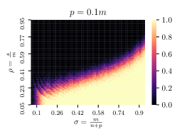
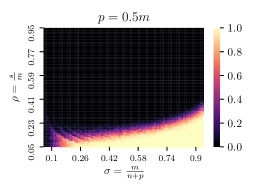
Figure 1: Phase transition curves for $p=0.1m$ (left) and $p=0.5m$ (right).

5.2 Noisy compressive sensing

If $\bm{x}$ can be interpreted as a noise vector, how does our model compare to noisy compressive sensing? Compressive sensing can be extended to the noisy case, which allows for the successful recovery of sparse signals under the presence of noise, assuming an upper bound on the noise level. In the rest of the section we examine how the proposed model, which incorporates both sparse and dense components, fares against this noisy variant.

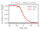
(a)

(b)

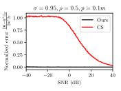
(c)

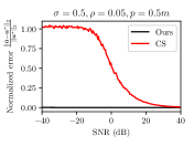
(d)

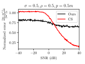
(e)

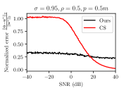
(f)

Figure 2: Normalized recovery error of $\bm{u}$ as the SNR varies (lower is better).

We, again, fix the number of columns in $\bm{B}$ to be $n=100$, and generate the matrices $\bm{A}\in\mathbb{R}^{m\times p}$ and $\bm{B}\in\mathbb{R}^{m\times n}$, as well as the vectors $\bm{x}^{*}\in\mathbb{R}^{p}$ and $\bm{u}^{*}\in\mathbb{R}^{n}$, as before. We define the signal-to-noise ratio as $\mathrm{SNR}=20\log_{10}\frac{\left|\left|\bm{u}^{*}\right|\right|_{2}}{\left|\left|\bm{x}^{*}\right|\right|_{2}}$, and iterate over the range $[-40\mathrm{dB},40\mathrm{dB}]$. To vary the SNR, we normalize both vectors and scale $\bm{u}^{*}$ by $10^{\frac{\mathrm{SNR}}{20}}$. For our proposed method, we solve the optimization of (4.2), whereas for noisy compressive sensing we solve

$$\hat{\bm{u}}=\arg\min_{\bm{u}}\left|\left|\bm{u}\right|\right|_{1},\quad\textrm{s.t.}\quad\left|\left|\bm{y}-\bm{B}\bm{u}\right|\right|_{2}\leq\left|\left|\bm{A}\bm{x}^{*}\right|\right|_{2},$$ (5.1)

and report the normalized error $\frac{\left|\left|\hat{\bm{u}}-\bm{u}^{*}\right|\right|_{2}}{\left|\left|\bm{u}^{*}\right|\right|_{2}}$ for the two methods averaging $100$ independent runs.

We present the SNR curves in Figure 2. As an initial observation, note that noisy compressive sensing, in every case, recovers a vector when the energy of the noise is less than that of the signal (for a SNR$>0$dB), and in most scenarios full recovery isn’t achieved unless the ratio is very large (SNR$>25$dB). That is expected, since the results for those settings assume an upper bound on the noise level. In contrast, our proposed model is able to recover both signals even when the norm of $\bm{x}$ is $100$ times larger than that of $\bm{u}$, at the cost of having access to the additional measurement matrix $\bm{A}$.

For low sparsity ratios (Figures 2(a) and (d)), we are able to recover both signals in every experiment using our model, whereas compressive sensing exhibits the behaviour we discussed above. Increasing the sparsity ratio while keeping the number of samples the same (Figures 2(b) and (e)) results in a significant reduction in performance for both models (note the different axis scaling for these figures). This is in line with both the results for noisy compressive sensing and our results presented in Section 4 (as well as the phase transition curves of the previous subsection). When the overlap between $\bm{A}$ and $\bm{B}$ is greater (Figure 2(e)) our model suffers a greater performance hit, as is expected from our analysis; note that noisy compressive sensing is unaffected by the relative size of $\bm{A}$ and $\bm{B}$, since it only makes assumptions about the noise level and not its span. Finally, we observe that increasing the number of measurements (Figures 2(c) and (f)) restores performance, in line with our analysis.

Remark: Note that the large sparsity ratios ($\rho=0.5$, corresponding to Figures 2(b), (c), (e), and (f)) violate our assumptions in Section 4 and recovery is not expected based on the transition curves of the previous subsection. However, we include them for illustration, as for smaller values of $\rho$ our model always recovered both vectors. As a key takeaway from this line of experimentation, we recommend the use of our model in every case where there is a structured interference with significant norm. In cases where the norm of the signal of interest is dominating (SNR$\approx 40$dB) and there is some form degeneracy (there is a large overlap between the signal spaces and $\bm{u}$ is barely sparse), noisy compressive sensing may be more appropriate.

5.3 Sensing with real data

In this section, we present experiments on real data using random sensing matrices. The real data we consider is the MNIST databse of handwritten digits [34, 35]. Through these experiments we want to (i) showcase the performance of our model on actual, real data and (ii) show the efficacy of our algorithm when using overcomplete sensing matrices.

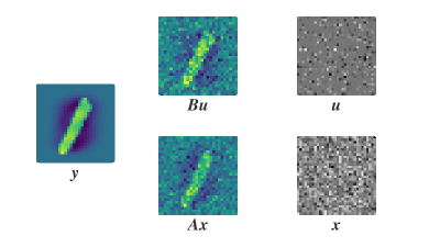
Figure 3: Decomposition of an MNIST image to its sparse and dense components.

In order to generate overcomplete dictionaries, we proceeded as follows: as MNIST images can be seen as vectors $\bm{y}\in\mathbb{R}^{784}$, we first generated a random orthogonal matrix in $\mathbb{R}^{784\times 784}$. We used half of the columns of that matrix as a base for $\bm{A}\in\mathbb{R}^{784\times 1024}$ and the other half for $\bm{B}\in\mathbb{R}^{784\times 1024}$; the rest of the columns were generated as linear combinations of each base. To avoid artificial orderings that might result when using certain optimizers, we conclude the matrix generation with random column permutations. These matrices, while in combination they do span $\mathbb{R}^{784}$, were not the generating model for the MNIST dataset. As such, we slightly alter the optimization problem of (4.2) to relax the exact reconstruction, yielding:

$$\underset{\bm{x},\bm{u}}{\min}\,\left|\left|\bm{A}\bm{x}+\bm{B}\bm{u}-\bm{y}\right|\right|_{2}^{2}+\mu\left|\left|\bm{A}\bm{x}\right|\right|_{2}^{2}+\lambda\left|\left|\bm{u}\right|\right|_{1}.$$ (5.2)

In our experiments, we use $\mu=3$ and $\lambda=0.01$. A visual decomposition of such an image is presented in Figure 3.

Both $\bm{u}$ and $\bm{x}$ have their expected properties: $\bm{u}$ is visibly sparse, with few nonzero elements and $\bm{x}$ has a fairly dense structure. Moreover, we observe that the component of $\bm{Ax}$ seems slightly more fainted compared to that of $\bm{Bu}$.

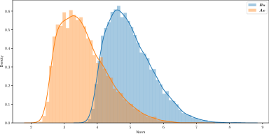
Figure 11: Euclidean norm distribution for the components $\bm{Ax}$ and $\bm{Bu}$ of MNIST images.

In order to further validate this observation we computed the both the Euclidean norm and the total variation for each component, as a proxy for smoothness, and plot the distributions of total variation in Figure 4. The distributions were computed using $10000$ training samples. The distribution of the Euclidean norm was very similar and can be found in the appendix, Figure 11. Observing the distributions of $\bm{Ax}$ and $\bm{Bu}$ we note that the distribution corresponding to the sparse component is skewed to higher values of total variation. This empirically validates the effectiveness of the smoothness regularization of (4.2), even when sensing using random matrices.

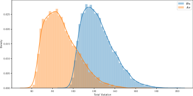
Figure 4: Total variation distribution for the components $\bm{Ax}$ and $\bm{Bu}$ of MNIST images.

As a final remark, we attempted to use $\bm{B}$ in a sparse coding framework in order to recover a sparse vector. However, in every instance the solver failed to converge and produce a sprase vector; this is, to an extent, expected as $\bm{B}$ was generated using only half the columns of an orthogonal matrix and therefore is unable to fully span the image space, failing to adequately represent all the images in the data set.

The main analysis in this paper is based on the measurement matrices and the Tikhonov matrix satisfying certain properties e.g. randomness is assumed in the matrix $\bm{B}$. However, in practice, efficient matrices are not always available, and random matrices might not optimal for every data set. Dictionary learning refers to the problem of learning $\bm{A}$ and $\bm{B}$ from data [1, 17, 29]. Based on unrolled neural architectures for the sparse coding model ($\bm{B}=0$) [58, 30], next section proposes an unrolled autoencoder to infer dense and sparse representations and learn dictionaries from data.

5.4 Dictionary learning based neural architecture for dense and sparse coding

We mitigate the drawbacks of convolutional sparse coding model in capturing a wide range of features from natural images by proposing dense and sparse dictionary learning; the framework learns a diverse set of features (i.e., smooth features via $\bm{A}$ and high-frequency features appearing sparsely through $\bm{B}$). We formulate the dense and sparse dictionary learning problem as minimizing the objective

$$\underset{\begin{subarray}{c}\bm{A},\bm{B},\bm{X},\bm{U}\end{subarray}}{\min}\ \frac{1}{2}\|\bm{Y}-\bm{A}\bm{X}-\bm{B}\bm{U}\|_{F}^{2}+\frac{1}{2\lambda_{x}}\|\bm{A}\bm{X}\|_{F}^{2}+\lambda_{u}\|\bm{U}\|_{1},$$ (5.3)

$$\bm{X}^{(l)},\bm{U}^{(l)}=\underset{\begin{subarray}{c}\bm{X},\bm{U}\end{subarray}}{\operatorname*{arg\,min}}\ \frac{1}{2}\|\bm{Y}-\bm{A}^{(l)}\bm{X}-\bm{B}^{(l)}\bm{U}\|_{F}^{2}+\frac{1}{2\lambda_{x}}\|\bm{A}^{(l)}\bm{X}\|_{F}^{2}+\lambda_{u}\|\bm{U}\|_{1}.$$ (5.4)

$$\bm{A}^{(l+1)},\bm{B}^{(l+1)}=\underset{\begin{subarray}{c}\bm{A},\bm{B}\end{subarray}}{\operatorname*{arg\,min}}\ \frac{1}{2}\|\bm{Y}-\bm{A}\bm{X}^{(l)}-\bm{B}\bm{U}^{(l)}\|_{F}^{2},$$ (5.5)

where as choice of design, we optimize only the reconstruction loss when updating the dictionaries. Based on the above alternating updates, we use deep unrolling to construct a unrolled neural network [58, 30], which we term the dense and sparse autoencoder (DenSaE), tailored to learning the dictionaries from the dense and sparse model. The encoder maps $\bm{Y}$ into a dense matrix $\bm{X}_{T}$ and a sparse one $\bm{U}_{T}$ using two sets of filters of $\bm{A}$ and $\bm{B}$ through a recurrent network. $\bm{A}$ encodes the smooth part of the data (low frequencies), and $\bm{B}$ encodes the details of the signal (high frequencies). The encoding is achieved by unrolling $T$ proximal gradient iterations shown below

$$\bm{X}_{t} =\bm{X}_{t-1}+\alpha_{x}(\bm{A}^{\text{T}}(\bm{Y}-(1+\frac{1}{\lambda_{x}})\bm{A}\bm{X}_{t-1}-\bm{B}\bm{U}_{t-1})),$$ (5.6)

$$\bm{U}_{t} =\mathcal{S}_{b}\big{(}\bm{U}_{t-1}+\alpha_{u}\bm{B}^{\text{T}}(\bm{Y}-\bm{A}\bm{X}_{t-1}-\bm{B}\bm{U}_{t-1})\big{)},$$

where $\alpha_{x}$ and $\alpha_{u}$ are step sizes, and $\mathcal{S}_{b}$, with $b=\alpha_{u}\lambda_{u}$, is the activation function; for non-negative sparse coding, the activation is $\text{ReLU}_{b}(z)=(z-b)\cdot\mathbbm{1}_{z\geq b}$, and for general sparse coding, it is $\text{Shrinkage}_{b}(z)=\text{ReLU}_{b}(z)-\text{ReLU}_{b}(-z)$ [58].

Having a non-informative prior on $\bm{A}\bm{x}$ in DenSaE implies that $\lambda_{x}\rightarrow\infty$. The parameters $\alpha_{x}$, $\alpha_{u}$, $\lambda_{u}$ are tuned via grid search. The decoder reconstructs the image using the generative model (i.e., $\bm{y}=\bm{A}\bm{x}_{T}+\bm{B}\bm{u}_{T}$). For classification, we use $\bm{u}_{T}$ and $\bm{x}_{T}$ as inputs to a linear classifier $\bm{C}$ that maps them to the predicted class $\bm{\hat{q}}$. The dictionaries $\bm{A}$ and $\bm{B}$ are learned via backpropagation. We remark that $b=\alpha_{u}\lambda_{u}$. A larger value of $b$ in the proximal mapping $\mathcal{S}_{b}$ enforces higher sparsity on $\bm{u}$, and a smaller value of $\lambda_{x}$ promotes smoothness on $\bm{A}\bm{x}$. We learn the dictionaries $\bm{A}$ and $\bm{B}$, as well as the classifier $\bm{C}$, by minimizing the weighted reconstruction (Rec.) and classification (Logistic) loss (i.e., $(1-\beta)$ Rec. + $\beta$ Logistic). Figure 5 shows the DenSaE architecture.

Figure 5: DenSaE. The vector $\bm{z}$ comprises the normalized features stacked plus a $1$ scalar for the classifier bias, $\mathcal{S}_{b}$ and $\mathcal{S}_{\text{\tiny max}}$ are the soft-thresholding and soft-max operators, respectively.

We examined the following questions

1. How do the discriminative, reconstruction, and denoising capabilities change as we vary the number of filters in $\bm{A}$ vs. $\bm{B}$?

2. What is the performance of DenSaE compared to sparse coding networks?

3. What data characteristics does the model capture?

As baselines, we trained two variants, $\text{CSCNet}_{\text{hyp}}$ and $\text{CSCNet}_{\text{LS}}$, of CSCNet [51], an architecture tailored to dictionary learning for the sparse coding problem $\bm{y}=\bm{B}\bm{u}$. In $\text{CSCNet}_{\text{hyp}}$, the bias is tuned as a shared hyper-parameter. In $\text{CSCNet}_{\text{LS}}$, we learn a different bias for each filter by minimizing the reconstruction loss. When the dictionaries are non-convolutional, we call the network SCNet.

5.4.1 DenSaE strikes a balance between discriminative capability and reconstruction

We study the case when DenSaE is trained on the MNIST dataset for joint reconstruction and classification. We show (i) how the explicit imposition of sparse and dense representations in DenSaE helps to balance discriminative and representation power, and (ii) that DenSaE outperforms SCNet. We warm start the training of the classifier using dictionaries obtained by first training the autoencoder, i.e., with $\beta=0$.

Characteristics of the representations $\bm{x}_{T}$ and $\bm{u}_{T}$: To evaluate the discriminative power of the representations learned by only training the autoencoder, we first trained the classifier given the representations (i.e., first train $\bm{A}$ and $\bm{B}$ with $\beta=0$, then train $\bm{C}$ with $\beta=1$). We call this disjoint training. Table 1 shows the classification accuracy (Acc.), $\ell_{2}$ reconstruction loss (Rec.), and the relative contributions, expressed as a percentage, of the dense or sparse representations to classification and reconstruction for disjoint training. Each column of $[\bm{A},\bm{B}]$, and of $\bm{C}$, corresponds to either a dense or a sparse feature. For reconstruction, we find the indices of the $50$ most important columns and report the proportion of these that represent dense features. For each of the $10$ classes (rows of $\bm{C}$), we find the indices of the $5$ most important columns (features) and compute the proportion of the total of $50$ indices that represent dense features. The first row of Table 1 shows the proportion of rows of $[\bm{A},\bm{B}]$ that represent dense features. Comparing this row, respectively to the third and fourth row reveals the importance of $\bm{x}$ for reconstruction, and of $\bm{u}$ for classification. Indeed, the Acc. and Rec. of Table 1 show that, as the proportion of dense features increases, DenSaE gains reconstruction capability but results in a lower classification accuracy. Moreover, in DenSaE, the most important features in classification are all from $\bm{B}$, and the contribution of $\bm{A}$ in reconstruction is greater than its percentage in the model, which clearly demonstrates that dense and sparse coding autoencoders balance discriminative and representation power.

Table 1: DenSaE’s performance on MNIST dataset from disjoint training. $\frac{\bm{A}}{\bm{A}+\bm{B}}$ is defined as $\frac{\#\ \text{columns of}\ \bm{A}}{\#\ \text{columns of}\ \bm{A}\ +\ \#\ \text{columns of}\ \bm{B}}\times 100$.

	$\begin{subarray}{c}\text{SCNet}_{\text{LS}}\end{subarray}$	$\begin{subarray}{c}\text{SCNet}_{\text{hyp}}\end{subarray}$	$\begin{subarray}{c}5\bm{A}\\ 395\bm{B}\end{subarray}$	$\begin{subarray}{c}25\bm{A}\\ 375\bm{B}\end{subarray}$	$\begin{subarray}{c}200\bm{A}\\ 200\bm{B}\end{subarray}$
$\frac{\bm{A}}{\bm{A}+\bm{B}}$	-	-	$1.25$%	$6.25$%	$50$%
Acc.	94.16  %	$98.32$%	$98.18$%	$98.18$%	$96.98$%
Rec.	1.95	$6.80$	$6.83$	$6.30$	$3.04$
$\bm{A}$ contribution to important class features	-	-	$0$%	$0$%	$0$%
$\bm{A}$ contribution to important rec. features	-	-	$8$%	$28$%	$58$%

Both Tables 1 and 2 show that DenSaE outperforms $\text{SCNet}_{\text{LS}}$ in classification and $\text{SCNet}_{\text{hyp}}$ in reconstruction. Specifically, for joint training, Table 2 (columns $2$,$3$ and row $J_{1}$) shows that DenSaE outperforms $\text{SCNet}_{\text{hyp}}$ for reconstruction ($32.61\ll 47.70$) while it is competitive for classification ($98.61>98.59$). Moreover, Table 2 (cols $1$, $3$ and $J_{0.75}$ and $J_{1}$) highlights that DenSAE has significantly better classification ($98.61>96.06$) and reconstruction ($32.61<71.20$) performances than $\text{SCNet}_{\text{LS}}$. Moreover, we observed that in the absence of noise, training $\text{SCNet}_{\text{LS}}$ results in dense features with small negative biases, hence, making its performance close to DenSaE with large number of atoms in $\bm{A}$. We see that $\text{SCNet}_{\text{LS}}$ in absence of a supervised classification loss fails to learn discriminative features useful for classification. On the other hand, enforcing sparsity in $\text{SCNet}_{\text{hyp}}$ suggests that sparse representations are useful for classification.

Table 2: DenSaE’s performance on MNIST dataset from
joint ($\text{J}_{\beta}$) training.

		$\begin{subarray}{c}\text{SCNet}_{\text{LS}}\end{subarray}$	$\begin{subarray}{c}\text{SCNet}_{\text{hyp}}\end{subarray}$	$\begin{subarray}{c}5\bm{A}\\ 395\bm{B}\end{subarray}$	$\begin{subarray}{c}25\bm{A}\\ 375\bm{B}\end{subarray}$	$\begin{subarray}{c}200\bm{A}\\ 200\bm{B}\end{subarray}$
	$\frac{\bm{A}}{\bm{A}+\bm{B}}$	-	-	$1.25$%	$6.25$%	$50$%
$\text{J}_{0.5}$	Acc.	$96.61$%	$97.97$%	$97.07$%	$97.68$%	$96.46$%
	Rec.	$2.01$	$0.87$	$0.58$	$0.58$	0.34
$\text{J}_{0.75}$	Acc.	$96.91$%	$98.18$%	$98.19$%	$98.23$%	$97.64$%
	Rec.	$2.17$	$1.24$	$0.75$	$1.11$	$0.51$
$\text{J}_{0.95}$	Acc.	$97.23$%	$98.51$%	$98.23$%	$98.44$%	$97.81$%
	Rec.	$4.48$	$1.03$	$1.22$	$1.32$	$0.67$
$\text{J}_{1}$	Acc.	$96.06$%	$98.59$%	98.61%	$98.56$%	$98.40$%
	Rec.	$71.20$	$47.70$	$32.61$	$30.20$	$25.57$

How do reconstruction and classification capabilities change as we vary $\beta$ in joint training?: In joint training of the autoencoder and the classifier, it is natural to expect that the reconstruction loss should increase compared to disjoint training. This is indeed the case for $\text{SCNet}_{\text{LS}}$; as we go from disjoint to joint training and as $\beta$ increases (Table 2), the reconstruction loss increases and classification accuracy has an overall increase. However, for $\beta<1$, joint training of both networks that enforce some sparsity on their representations, $\text{SCNet}_{\text{hyp}}$ and DenSaE, improves reconstruction and classification.

For purely discriminative training ($\beta=1$), DenSaE outperforms both $\text{SCNet}_{\text{LS}}$ and $\text{SCNet}_{\text{hyp}}$ in classification accuracy and representation capability. We speculate that this likely results from the fact that, by construction, the encoder from DenSaE seeks to produce two sets of representations: namely a dense one, mostly important for reconstruction and a sparse one, useful for classification. In some sense, the dense component acts as a prior that promotes good reconstruction.

Figure 6: Visualization of a test image for $\tau=50$. a) DenSaE $(4\bm{A},60\bm{B})$, b) $\text{CSCNet}_{\text{LS}}$. $\bm{B}\bm{u}$ images are scaled and plotted with a different colormap for visualization purposes.

5.4.2 Denoising

We trained DenSaE for supervised image denoising when $\beta=0$ using BSD432 and tested it on BSD68 [40]. All the networks are trained for $250$ epochs using the ADAM optimizer and the filters are initialized using the random Gaussian distribution. The initial learning rate is set to $10^{-4}$ and then decayed by $0.8$ every $50$ epochs. We set $\epsilon$ of the optimizer to be $10^{-3}$ for stability. At every iteration, a random patch of size $128\times 128$ is cropped from the training image and zero-mean Gaussian noise is added to it with the corresponding noise level. We varied the ratio of number of filters in $\bm{A}$ and $\bm{B}$ as the overall number of filters was kept constant. We evaluate the model in the presence of Gaussian noise with standard deviation of $\tau=\{15,25,50,75\}$.

Table 3: DenSaE’s denoising performance
on BSD68 as the ratio of filters changes.

$\tau$	$1\bm{A}63\bm{B}$	$4\bm{A}60\bm{B}$	$8\bm{A}56\bm{B}$	$16\bm{A}48\bm{B}$	$32\bm{A}32\bm{B}$
$15$	30.21	30.18	30.18	30.14	29.89
$25$	27.70	27.70	27.65	27.56	27.26
$50$	24.81	24.81	24.43	24.44	23.68
$75$	23.31	23.33	23.09	22.09	20.09

Ratio of number of filters in $\bm{A}$ and $\bm{B}$: Unlike reconstruction, Table 3 shows that the smaller the number of filters associated with $\bm{A}$, the better DenSaE can denoise images. We hypothesize that this is a direct consequence of our findings from Section 4 that if the column spaces of $\bm{A}$ and $\bm{B}$ are suitably unaligned, the easier is the recovery $\bm{x}$ and $\bm{u}$.

Table 4: DenSaE vs. CSCNet
on BSD68.

$\tau$	DenSaE	$\text{CSCNet}_{\text{hyp}}$	$\text{CSCNet}_{\text{LS}}$
$15$	30.21	30.12	30.34
$25$	27.70	27.51	27.75
$50$	24.81	24.54	24.81
$75$	23.33	22.83	23.32

Dense and sparse vs. sparse coding: Table 4 shows that DenSaE (best network from Table 3) denoises images better than $\text{CSCNet}_{\text{hyp}}$, suggesting that the dense and sparse coding model represents images better than sparse coding.

Dictionary characteristics: Figure 6(a) shows the decomposition of a noisy test image ($\tau=50$) by DenSaE. The figure demonstrates that $\bm{A}\bm{x}$ captures low-frequency content while $\bm{B}\bm{u}$ captures high-frequency details (edges). This is corroborated by the smoothness of the filters associated with $\bm{A}$, and the Gabor-like nature of those associated with $\bm{B}$ [41]. We observed similar performance when we tuned $\lambda_{x}$, and found that, as $\lambda_{x}$ decreases, $\bm{A}\bm{x}$ captures a lower frequencies, and $\bm{B}\bm{u}$ a broader range.

CSCNet deviates from sparse coding and implicitly learns $\bm{A}\bm{x}+\bm{B}\bm{u}$ model in the presence of noise: By training the biases, $\text{CSCNet}_{\text{LS}}$ deviates from the sparse coding model; the neural network’s bias is directly related to the sparsity enforcing hyper-parameter $\lambda_{u}$. The larger this bias, the sparser the representations. We observed that $\text{CSCNet}_{\text{LS}}$ automatically segments filters into three groups: one with small bias, one with intermediate ones, and a third with large values (see  10). We found that the feature maps associated with the large bias values are all zero. Moreover, the majority of features are associated with intermediate bias values, and are sparse, in contrast to the small number of feature maps with small bias values, which are dense. We call the dictionary atoms, corresponding such small biases, implicit $\bm{A}$. Similarly, dictionary atoms with moderate biases can be seen as implicit $\bm{B}$.

These observations suggest that autoencoders implementing the sparse coding model ($\bm{y}=\bm{B}\bm{u}$), when learning the biases by minimizing reconstruction error, implicitly perform two functions. First, they select the optimal number of filters. Second, they partition the filters into two groups: one that yields a dense representation of the input, and another that yields a sparse one. In other words, the architectures trained in this manner implicitly learn the dense and sparse coding model. Figure 6(b) shows the filters.

The above-mentioned interpretation of CSCNet with learned biases offers to revisit the optimization-based model used to construct the autoencoder; if the network implicitly learns a bipartite representation, why not explicitly model that structure? Through our experiments we showed that doing so leads to increased performance, the recovered dictionaries and representations do not deviate from their expected behavior, and the resulting network is more interpretable, as we can directly visualize and analyze each component.

6 Conclusions

This paper proposed a novel dense and sparse coding model for a flexible representation of a signal as $\bm{y}=\bm{A}\bm{x}+\bm{B}\bm{u}$. Our first result gives a verifiable condition that guarantees uniqueness of the model. Our second result uses tools from anisotropic compressed sensing to show that, with sufficiently many linear measurements, a convex program with $\ell_{1}$ and $\ell_{2}$ regularizations can recover the components $\bm{x}$ and $\bm{u}$ uniquely with high probability. Numerical experiments on synthetic and real data confirm our observations.

We proposed a dense and sparse autoencoder, DenSaE, tailored to dictionary learning for the $\bm{A}\bm{x}+\bm{B}\bm{u}$ model. DenSaE, naturally decomposing signals into low- and high-frequency components, provides a balance between learning dense representations that are useful for reconstruction and discriminative sparse representations. We showed the superiority of DenSaE to sparse autoencoders for data reconstruction and its competitive performance in classification.

Data availability

The data underlying section 5.4 (the image denoising data BSD dataset, our trained models and codes) are available at https://github.com/btolooshams/densaee.

Author contributions

Abiy Tasissa, Emmanouil Theodosis and Demba Ba studied the model in (1.1) and worked on the theoretical analysis presented in Section 4. Emmanouil Theodosis conducted all the experiments in Sections 5.1, 5.2 and 5.3. Bahareh Tolooshams designed and conducted the experiments in Section 5.4 for dictionary learning-based neural architectures. All authors contributed to the writing of the manuscript.

Appendix A Classification and Image Denoising

We warm start the networks by training the autoencoder for $150$ epochs using the ADAM optimizer where the weights are initialized with the random Gaussian distribution.

Table 5: Network parameters for MNIST classification experiment.

	DenSaE	$\text{CSCNet}_{\text{hyp}}$	$\text{CSCNet}_{\text{LS}}$
# dictionary atoms	$400$
Image size	$28$$\times$$28$
# training examples	$50{,}000$ MNIST
# validation examples	$10{,}000$ MNIST
# testing examples	$10{,}000$ MNIST
# trainable parameters in the autoencoder	$313{,}600$	$313{,}600$	$314{,}000$
# trainable parameters in the classifier	$4{,}010$	$4{,}010$	$4{,}010$
$\mathcal{S}(.)$	ReLU
Encoder layers $T$	$15$
$\alpha_{u}$	$0.02$
$\alpha_{x}$	0.02	-	-
$\lambda_{u}^{\text{init}}$	$0.5$	$0.5$	$0.0$

The learning rate is set to $10^{-3}$. We set $\epsilon$ of the optimizer to be $10^{-15}$ and used batch size of $16$. For disjoint classification training, we trained for $1{,}000$ epochs, and for joint classification training, the network is trained for $500$ epochs. All the networks use FISTA [6] within their encoder for faster sparse coding. Table 5 lists the parameters of the different networks. Figure 7 visualizes the most important atoms for reconstruction and classification for disjoint training.

$\bm{B}$ rec. $\bm{B}$ class

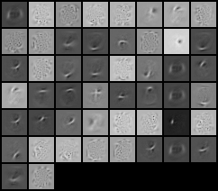
(a) $\text{SCNet}_{\text{LS}}$

$\bm{B}$ rec. $\bm{B}$ class

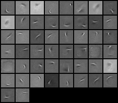
(b) $\text{SCNet}_{\text{hyp}}$

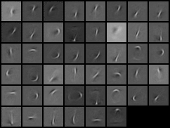
$\bm{A}$ rec. $\bm{B}$ rec. $\bm{B}$ class

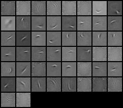
(c) DenSaE $5\bm{A}395\bm{B}$

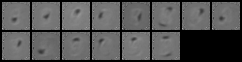
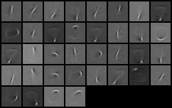
$\bm{A}$ rec. $\bm{B}$ rec. $\bm{B}$ class

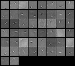
(d) DenSaE $25\bm{A}375\bm{B}$

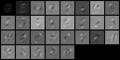
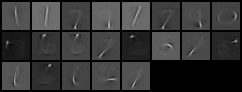
$\bm{A}$ rec. $\bm{B}$ rec. $\bm{B}$ class

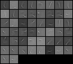
(e) DenSaE $200\bm{A}200\bm{B}$

Figure 7: Most important atoms of the dictionary used for reconstruction (rec.) and classification (class.) for disjoint training.

Figure 8 visualizes the reconstruction of MNIST test image for the disjoint training, where the autoencoder is trained for pure reconstruction (i.e., $\beta=0$).

$\bm{y}$

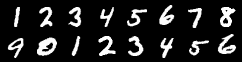
(a) Original

$\hat{\bm{y}}$

(b) $\text{SCNet}_{\text{LS}}$

$\hat{\bm{y}}$

(c) $\text{SCNet}_{\text{hyp}}$

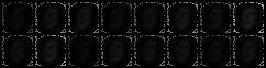
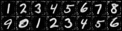
$\bm{A}\bm{x}$ $\bm{B}\bm{u}$ $\hat{\bm{y}}$

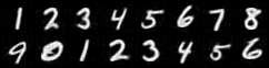
(d) DenSaE $5\bm{A}395\bm{B}$

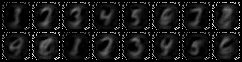
$\bm{A}\bm{x}$ $\bm{B}\bm{u}$ $\hat{\bm{y}}$

(e) DenSaE $25\bm{A}375\bm{B}$

$\bm{A}\bm{x}$ $\bm{B}\bm{u}$ $\hat{\bm{y}}$

(f) DenSaE $200\bm{A}200\bm{B}$

Figure 8: Reconstruction of MNIST test images for disjoint classification.

The figure shows that $\text{SCNet}_{\text{LS}}$ has the best reconstruction among all, and the second best is $\text{DenSaE}_{\begin{subarray}{c}200\bm{A},200\bm{B}\end{subarray}}$, having the highest number of $\bm{A}$ atoms. Figures 9 visualizes the reconstruction of MNIST test image for the joint training when $\beta=1$. Notably, in this case, the reconstructions from $\text{SCNet}_{\text{LS}}$ do not look like the original image. On the other hand, DenSaE even with $\beta=1$ is able to reconstruct the image very well. In addition, the figures show how $\bm{A}\bm{x}$ and $\bm{B}\bm{u}$ are contribution for reconstruction for DenSaE.

$\bm{y}$

(a) Original

$\hat{\bm{y}}$

(b) $\text{SCNet}_{\text{LS}}$

$\hat{\bm{y}}$

(c) $\text{SCNet}_{\text{hyp}}$

$\bm{A}\bm{x}$ $\bm{B}\bm{u}$ $\hat{\bm{y}}$

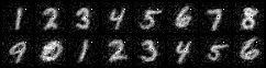
(d) DenSaE $5\bm{A}395\bm{B}$

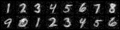
$\bm{A}\bm{x}$ $\bm{B}\bm{u}$ $\hat{\bm{y}}$

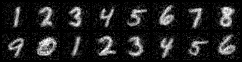
(e) DenSaE $25\bm{A}375\bm{B}$

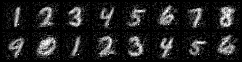
$\bm{A}\bm{x}$ $\bm{B}\bm{u}$ $\hat{\bm{y}}$

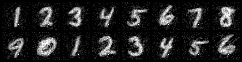
(f) DenSaE $200\bm{A}200\bm{B}$

Figure 9: Reconstruction of MNIST test images for joint classification when $\beta=1$.

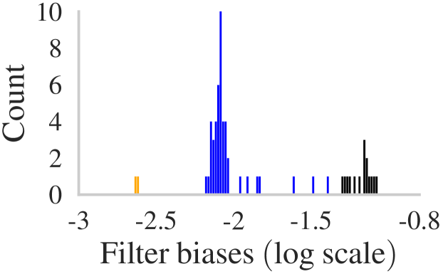
(a) $\tau=15$

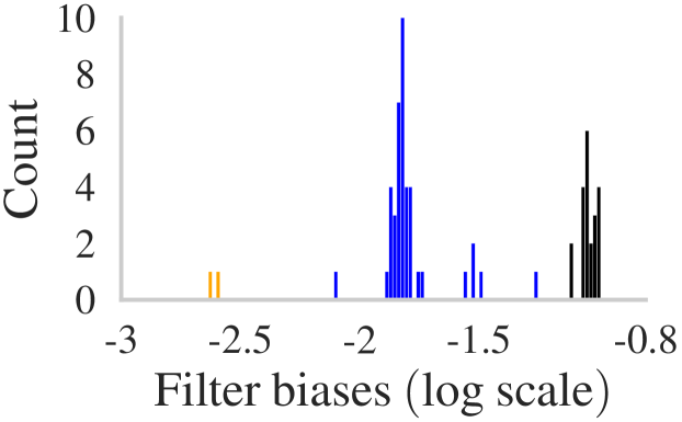
(b) $\tau=25$

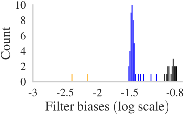
(c) $\tau=50$

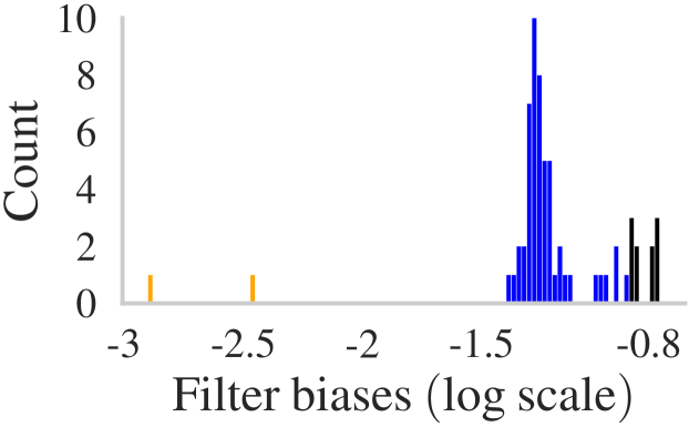
(d) $\tau=75$

Figure 10: Histogram of biases from $\text{CSCNet}_{\text{LS}}$ for various noise levels.

We note that as our network is non-convolutional, we do not compare it to the state-of-the-art, a convolutional network. We do not compare our results with the network in [49] as that work does not report reconstruction loss and it involves a sparsity enforcing loss that change the learning behaviour.

Table 6: Network parameters for natural image denoising experiments.

		DenSaE	$\text{CSCNet}_{\text{hyp}}$	$\text{CSCNet}_{\text{LS}}$
# filters		$64$
Filter size		$7$$\times$$7$
Strides		$5$
Patch size		$128$$\times$$128$
# training examples		$432$ BSD432
# testing examples		$68$ BSD68
# trainable parameters		$3{,}136$	$3{,}136$	$3{,}200$
$\mathcal{S}(.)$		Shrinkage
Encoder layers $T$		$15$
$\alpha_{u}$		$0.1$
$\alpha_{x}$		0.1	-	-
$\lambda_{u}^{\text{init}}$	$\tau=15$	$0.085$	$0.085$	$0.1$
	$\tau=25$	$0.16$	$0.16$	$0.1$
	$\tau=50$	$0.36$	$0.36$	$0.1$
	$\tau=75$	$0.56$	$0.56$	$0.1$

For denoising, all the trained networks implement FISTA for faster sparse coding. Table 6 lists the parameters of the different networks. Moreover, Figure 10 shows the histogram of learned biases by $\mathrm{CSCNet}_{\mathrm{LS}}$ for various noise levels. We note that compared to CSCNet, which has $63$K trainable parameters, all the trained networks including $\text{CSCNet}^{\text{LS}}$ have $20$x fewer trainable parameters. We attribute the difference in performance, compared to the results reported in the CSCNet paper, to this large difference in the number of trainable parameters and the usage of a larger dataset.

Appendix B Euclidean norm distribution

References

- Agarwal et al. [2014] A. Agarwal, A. Anandkumar, P. Jain, P. Netrapalli, and R. Tandon. Learning sparsely used overcomplete dictionaries. In M. F. Balcan, V. Feldman, and C. Szepesvári, editors, Proc the 27th Conference on Learning Theory, volume 35 of Proceedings of Machine Learning Research, pages 123–137, Barcelona, Spain, 13–15 Jun 2014. PMLR.
- Agarwal et al. [2016] A. Agarwal, A. Anandkumar, P. Jain, P. Netrapalli, and R. Tandon. Learning sparsely used overcomplete dictionaries via alternating minimization. SIAM Journal on Optimization, 26:2775–2799, 2016.
- Aharon et al. [2006] M. Aharon, M. Elad, and A. Bruckstein. -svd: An algorithm for designing overcomplete dictionaries for sparse representation. IEEE Transactions on signal processing, 54(11):4311–22, 2006.
- Aujol et al. [2003] J.-F. Aujol, G. Aubert, L. Blanc-Féraud, and A. Chambolle. Image decomposition: application to textured images and SAR images. Technical Report RR-4704, INRIA, Jan. 2003. URL https://hal.inria.fr/inria-00071882.
- Baraniuk et al. [2008] R. Baraniuk, M. Davenport, R. DeVore, and M. Wakin. A simple proof of the restricted isometry property for random matrices. Constructive Approximation, 28(3):253–263, 2008.
- Beck and Teboulle [2009] A. Beck and M. Teboulle. A fast iterative shrinkage-thresholding algorithm for linear inverse problems. SIAM journal on imaging sciences, 2(1):183–202, 2009.
- Bertalmio et al. [2003] M. Bertalmio, L. Vese, G. Sapiro, and S. Osher. Simultaneous structure and texture image inpainting. IEEE transactions on image processing, 12(8):882–889, 2003.
- Björck and Golub [1973] A. Björck and G. H. Golub. Numerical methods for computing angles between linear subspaces. Mathematics of computation, 27(123):579–594, 1973.
- Bobin et al. [2007] J. Bobin, J.-L. Starck, J. M. Fadili, Y. Moudden, and D. L. Donoho. Morphological component analysis: An adaptive thresholding strategy. IEEE transactions on image processing, 16(11):2675–2681, 2007.
- Candes et al. [2005] E. Candes, M. Rudelson, T. Tao, and R. Vershynin. Error correction via linear programming. In 46th Annual IEEE Symposium on Foundations of Computer Science (FOCS’05), pages 668–681. IEEE, 2005.
- Candes [2008] E. J. Candes. The restricted isometry property and its implications for compressed sensing. Comptes rendus mathematique, 346(9-10):589–592, 2008.
- Candes and Plan [2011] E. J. Candes and Y. Plan. A probabilistic and ripless theory of compressed sensing. IEEE transactions on information theory, 57(11):7235–7254, 2011.
- Candes and Tao [2005] E. J. Candes and T. Tao. Decoding by linear programming. IEEE transactions on information theory, 51(12):4203–4215, 2005.
- Candes and Tao [2006] E. J. Candes and T. Tao. Near-optimal signal recovery from random projections: Universal encoding strategies? IEEE transactions on information theory, 52(12):5406–5425, 2006.
- Candès et al. [2011] E. J. Candès, X. Li, Y. Ma, and J. Wright. Robust principal component analysis? Journal of the ACM (JACM), 58(3):1–37, 2011.
- Chang and Chiang [2002] C.-I. Chang and S.-S. Chiang. Anomaly detection and classification for hyperspectral imagery. IEEE transactions on geoscience and remote sensing, 40(6):1314–1325, 2002.
- Chatterji and Bartlett [2017] N. S. Chatterji and P. L. Bartlett. Alternating minimization for dictionary learning: Local convergence guarantees. arXiv:1711.03634, pages 1–26, 2017.
- Chen et al. [2001] S. S. Chen, D. L. Donoho, and M. A. Saunders. Atomic decomposition by basis pursuit. SIAM review, 43(1):129–159, 2001.
- Davis et al. [1997] G. Davis, S. Mallat, and M. Avellaneda. Adaptive greedy approximations. Constructive approximation, 13(1):57–98, 1997.
- Donoho and Elad [2003] D. L. Donoho and M. Elad. Optimally sparse representation in general (nonorthogonal) dictionaries via minimization. Proc. the National Academy of Sciences, 100(5):2197–2202, 2003.
- Donoho and Huo [2001] D. L. Donoho and X. Huo. Uncertainty principles and ideal atomic decomposition. IEEE transactions on information theory, 47(7):2845–2862, 2001.
- Donoho and Stark [1989] D. L. Donoho and P. B. Stark. Uncertainty principles and signal recovery. SIAM Journal on Applied Mathematics, 49(3):906–931, 1989.
- Donoho et al. [2005] D. L. Donoho, M. Elad, and V. N. Temlyakov. Stable recovery of sparse overcomplete representations in the presence of noise. IEEE Transactions on information theory, 52(1):6–18, 2005.
- Elad and Bruckstein [2002] M. Elad and A. M. Bruckstein. A generalized uncertainty principle and sparse representation in pairs of bases. IEEE Transactions on Information Theory, 48(9):2558–2567, 2002.
- Elad et al. [2005] M. Elad, J.-L. Starck, P. Querre, and D. L. Donoho. Simultaneous cartoon and texture image inpainting using morphological component analysis (mca). Applied and computational harmonic analysis, 19(3):340–358, 2005.
- Eldar et al. [2010] Y. C. Eldar, P. Kuppinger, and H. Bolcskei. Block-sparse signals: Uncertainty relations and efficient recovery. IEEE Transactions on Signal Processing, 58(6):3042–3054, 2010.
- Flinth [2016] A. Flinth. Optimal choice of weights for sparse recovery with prior information. IEEE Transactions on Information Theory, 62(7):4276–4284, 2016.
- Friedlander et al. [2011] M. P. Friedlander, H. Mansour, R. Saab, and Ö. Yilmaz. Recovering compressively sampled signals using partial support information. IEEE Transactions on Information Theory, 58(2):1122–1134, 2011.
- Garcia-Cardona and Wohlberg [2018] C. Garcia-Cardona and B. Wohlberg. Convolutional dictionary learning: A comparative review and new algorithms. IEEE Transactions on Computational Imaging, 4(3):366–81, Sept. 2018. doi: 10.1109/TCI.2018.2840334.
- Gregor and Lecun [2010] K. Gregor and Y. Lecun. Learning fast approximations of sparse coding. In Proc. International Conference on Machine Learning (ICML), pages 399–406, 2010.
- Gribonval and Nielsen [2003] R. Gribonval and M. Nielsen. Sparse representations in unions of bases. IEEE transactions on Information theory, 49(12):3320–3325, 2003.
- Kueng and Gross [2014] R. Kueng and D. Gross. Ripless compressed sensing from anisotropic measurements. Linear Algebra and its Applications, 441:110–123, 2014.
- Kuppinger et al. [2011] P. Kuppinger, G. Durisi, and H. Bolcskei. Uncertainty relations and sparse signal recovery for pairs of general signal sets. IEEE transactions on information theory, 58(1):263–277, 2011.
- [34] Y. LeCun. The mnist database of handwritten digits. Accessed: 2022-08-22.
- LeCun et al. [1998] Y. LeCun, L. Bottou, Y. Bengio, and P. Haffner. Gradient-based learning applied to document recognition. Proceedings of the IEEE, 86(11):2278–2324, 1998.
- Lian et al. [2018] L. Lian, A. Liu, and V. K. Lau. Weighted lasso for sparse recovery with statistical prior support information. IEEE Transactions on Signal Processing, 66(6):1607–1618, 2018.
- Mairal et al. [2011] J. Mairal, F. Bach, and J. Ponce. Task-driven dictionary learning. IEEE transactions on pattern analysis and machine intelligence, 34(4):791–804, 2011.
- Mallat and Yu [2010] S. Mallat and G. Yu. Super-resolution with sparse mixing estimators. IEEE transactions on image processing, 19(11):2889–2900, 2010.
- Mansour and Saab [2017] H. Mansour and R. Saab. Recovery analysis for weighted l1-minimization using the null space property. Applied and Computational Harmonic Analysis, 43(1):23–38, 2017.
- Martin et al. [2001] D. Martin, C. Fowlkes, D. Tal, and J. Malik. A database of human segmented natural images and its application to evaluating segmentation algorithms and measuring ecological statistics. In Proc. 8th Int’l Conf. Computer Vision, volume 2, pages 416–423, July 2001.
- Mehrotra et al. [1992] R. Mehrotra, K. Namuduri, and N. Ranganathan. Gabor filter-based edge detection. Pattern Recognition, 25(12):1479–94, 1992. ISSN 0031-3203.
- Monga et al. [2019] V. Monga, Y. Li, and Y. C. Eldar. Algorithm unrolling: Interpretable, efficient deep learning for signal and image processing. arXiv preprint arXiv:1912.10557, 2019.
- Nguyen and Tran [2013] N. H. Nguyen and T. D. Tran. Exact recoverability from dense corrupted observations via l1-minimization. IEEE transactions on information theory, 59(4):2017–2035, 2013.
- Olshausen and Field [1997] B. A. Olshausen and D. J. Field. Sparse coding with an overcomplete basis set: A strategy employed by v1? Vision research, 37(23):3311–3325, 1997.
- Oymak et al. [2012] S. Oymak, M. A. Khajehnejad, and B. Hassibi. Recovery threshold for optimal weight l1 minimization. In 2012 IEEE International Symposium on Information Theory Proceedings, pages 2032–2036. IEEE, 2012.
- Pati et al. [1993] Y. C. Pati, R. Rezaiifar, and P. S. Krishnaprasad. Orthogonal matching pursuit: Recursive function approximation with applications to wavelet decomposition. In Proceedings of 27th Asilomar conference on signals, systems and computers, pages 40–44. IEEE, 1993.
- Peng et al. [2016] X. Peng, C. Lu, Z. Yi, and H. Tang. Connections between nuclear-norm and frobenius-norm-based representations. IEEE transactions on neural networks and learning systems, 29(1):218–224, 2016.
- Pope et al. [2013] G. Pope, A. Bracher, and C. Studer. Probabilistic recovery guarantees for sparsely corrupted signals. IEEE transactions on information theory, 59(5):3104–3116, 2013.
- Rolfe and LeCun [2013] J. T. Rolfe and Y. LeCun. Discriminative recurrent sparse auto-encoders. arXiv preprint arXiv:1301.3775, 2013.
- Shen et al. [2022] B. Shen, R. R. Kamath, H. Choo, and Z. Kong. Robust tensor decomposition based background/foreground separation in noisy videos and its applications in additive manufacturing. IEEE Transactions on Automation Science and Engineering, 2022.
- Simon and Elad [2019] D. Simon and M. Elad. Rethinking the csc model for natural images. In Proc. Advances in Neural Information Processing Systems, pages 2271–2281, 2019.
- Starck et al. [2004] J.-L. Starck, M. Elad, and D. L. Donoho. Redundant multiscale transforms and their application for morphological component separation. Advances in Imaging and Electron Physics, 132:287–348, 2004.
- Starck et al. [2005] J.-L. Starck, M. Elad, and D. L. Donoho. Image decomposition via the combination of sparse representations and a variational approach. IEEE transactions on image processing, 14(10):1570–1582, 2005.
- Studer and Baraniuk [2014] C. Studer and R. G. Baraniuk. Stable restoration and separation of approximately sparse signals. Applied and Computational Harmonic Analysis, 37(1):12–35, 2014.
- Studer et al. [2011] C. Studer, P. Kuppinger, G. Pope, and H. Bolcskei. Recovery of sparsely corrupted signals. IEEE Transactions on Information Theory, 58(5):3115–3130, 2011.
- Sulam et al. [2019] J. Sulam, A. Aberdam, A. Beck, and M. Elad. On multi-layer basis pursuit, efficient algorithms and convolutional neural networks. IEEE Transactions on Pattern Analysis and Machine Intelligence, pages 1–1, 2019. ISSN 1939-3539. doi: 10.1109/TPAMI.2019.2904255.
- Tikhonov et al. [1995] A. N. Tikhonov, A. Goncharsky, V. Stepanov, and A. G. Yagola. Numerical methods for the solution of ill-posed problems, volume 328. Springer Science & Business Media, 1995.
- Tolooshams et al. [2020] B. Tolooshams, S. Dey, and D. Ba. Deep residual autoencoders for expectation maximization-inspired dictionary learning. IEEE Transactions on Neural Networks and Learning Systems, pages 1–15, 2020. doi: 10.1109/TNNLS.2020.3005348.
- Tropp [2004] J. A. Tropp. Greed is good: Algorithmic results for sparse approximation. IEEE Transactions on Information theory, 50(10):2231–2242, 2004.
- Tropp and Gilbert [2007] J. A. Tropp and A. C. Gilbert. Signal recovery from random measurements via orthogonal matching pursuit. IEEE Transactions on information theory, 53(12):4655–4666, 2007.
- Vaswani and Lu [2010] N. Vaswani and W. Lu. Modified-cs: Modifying compressive sensing for problems with partially known support. IEEE Transactions on Signal Processing, 58(9):4595–4607, 2010.
- Vese and Osher [2003] L. A. Vese and S. J. Osher. Modeling textures with total variation minimization and oscillating patterns in image processing. Journal of scientific computing, 19(1):553–572, 2003.
- Wright and Ma [2010] J. Wright and Y. Ma. Dense error correction via l1-minimization. IEEE Transactions on Information Theory, 56(7):3540–3560, 2010.
- Yan et al. [2017] H. Yan, K. Paynabar, and J. Shi. Anomaly detection in images with smooth background via smooth-sparse decomposition. Technometrics, 59(1):102–114, 2017.
- Zazo et al. [2019] J. Zazo, B. Tolooshams, and D. Ba. Convolutional dictionary learning in hierarchical networks. In Proc. 2019 IEEE 8th International Workshop on Computational Advances in Multi-Sensor Adaptive Processing (CAMSAP), pages 131–135. IEEE, 2019.
- Zhang et al. [2014] H. Zhang, Z. Yi, and X. Peng. flrr: fast low-rank representation using frobenius-norm. Electronics Letters, 50(13):936–938, 2014.
- Zhou et al. [2012] X. Zhou, C. Yang, and W. Yu. Moving object detection by detecting contiguous outliers in the low-rank representation. IEEE transactions on pattern analysis and machine intelligence, 35(3):597–610, 2012.