Decomposable Families of Itemsets

Abstract

The problem of selecting a small, yet high quality subset of patterns from a larger collection of itemsets has recently attracted lot of research. Here we discuss an approach to this problem using the notion of decomposable families of itemsets. Such itemset families define a probabilistic model for the data from which the original collection of itemsets has been derived from. Furthermore, they induce a special tree structure, called a junction tree, familiar from the theory of Markov Random Fields. The method has several advantages. The junction trees provide an intuitive representation of the mining results. From the computational point of view, the model provides leverage for problems that could be intractable using the entire collection of itemsets. We provide an efficient algorithm to build decomposable itemset families, and give an application example with frequency bound querying using the model. Empirical results show that our algorithm yields high quality results.

1 Introduction

Frequent itemset discovery has been a central research theme in the data mining community ever since the idea was introduced by Agrawal et. al [1]. Over the years, scalability of the problem has been the most studied aspect, and several very efficient algorithms for finding all frequent itemsets have been introduced, Apriori [2] or FP-growth [3] among others. However, it has been argued recently that while efficiency of the mining task is no longer a bottleneck, there is still a strong need for methods that derive compact, yet high quality results with good application properties [4].

In this study we propose the notion of decomposable families of itemsets to address this need. The general idea is to build a probabilistic model of a given dataset $D$ using a small well-chosen subset of itemsets $\mathcal{G}$ from a given candidate family $\mathcal{F}$. The candidate family $\mathcal{F}$ may be generated from $D$ using some frequent itemset mining algorithm. A special aspect of a decomposable family is that it induces a type of tree, called a junction tree, a well-known concept from the theory of Markov Random Fields [5].

As a simple example, consider a dataset $D$ with six attributes $a,\ldots,f$, and a family $\mathcal{G}$ = {$bcd$, $bcf$, $ab$, $ce$, $bc$, $bd$, $cd$, $bf$, $cf$, $a$, $b$, $c$, $d$, $e$, $f$}. The family $\mathcal{G}$ can be represented as the junction tree shown in Figure 1 such that the nodes in the tree are the maximal itemsets in $\mathcal{G}$. Furthermore, the junction tree defines a decomposable model of the dataset $D$.

$$p(abcdef)=\frac{p(ab)p(bcd)p(bcf)p(ce)}{p(b)p(bc)p(c)}$$

Figure 1: An example of a junction tree and the corresponding distribution decomposition.

Using decomposable itemset families has several notable advantages. First of all, the following junction tree graphs provide an extremely intuitive representation of the mining results. This is a significant advantage over many other itemset selection methods, as even small mining results of, say 50 itemsets, can be hard for humans to grasp as a whole, if just plainly enumerated. Second, from the computational point of view, decomposable families of itemsets provide leverage for accurately solving problems that could be intractable using the entire result set. Such problems include, for instance, querying for frequency bounds of arbitrary attribute combinations. Third, the statistical nature of the overall model enable to incorporated regularization terms, like BIC, AIC, or MDL to select only itemsets that reflect true dependencies between attributes.

In this study we provide an efficient algorithm to build decomposable itemset families while optimizing the likelihood of the model. We also demonstrate how to use decomposable itemset families to execute frequency bound querying, an intractable problem in the general case. We provide empirical results showing that our algorithm works well in practice.

The rest of the paper is organized as follows. Preliminaries are given in Section 2 and the concept of decomposable models are defined in Section 3. A greedy search algorithm is given in Section 4. Section 6 is devoted to experiments. We present the related work in Section 7 and conclude the paper with discussion in Section 8. The proofs for the theorems in this paper are provided in [6].

2 Preliminaries and Notations

In this section we describe the notation and the background definitions that are used in the subsequent sections.

A binary dataset $D$ is a collection of $N$ transactions, binary vectors of length $K$. The dataset can be viewed as a binary matrix of size $N\times K$. We denote the number of transactions by ${\left|D\right|}=N$. The $i$th element of a random transaction is represented by an attribute $a_{i}$, a Bernoulli random variable. We denote the collection of all the attributes by $A=\left\{a_{1},\ldots,a_{K}\right\}$. An itemset $X=\left\{x_{1},\ldots,x_{L}\right\}\subseteq A$ is a subset of attributes. We will often use the dense notation $X={x_{1}}\cdots{x_{L}}$.

Given an itemset $X$ and a binary vector $v$ of length $L$, we use the notation $p\left(X=v\right)$ to express the probability of $p\left(x_{1}=v_{1},\ldots,x_{L}=v_{L}\right)$. If $v$ contains only 1s, then we will use the notation $p\left(X=1\right)$.

Given a binary dataset $D$ we define $q_{D}$ to be an empirical distribution,

$$q_{D}\left(A=v\right)={\left|\left\{t\in D;t=v\right\}\right|}/{\left|D\right|}.$$

We define the frequency of an itemset to be $fr\mathopen{}\left(X\right)=q_{D}\left(X=1\right)$. The entropy of an itemset $X={x_{1}}\cdots{x_{L}}$ given $D$, denoted by $H\mathopen{}\left(X;D\right)$, is defined as

$$H\mathopen{}\left(X;D\right)=-\sum_{v\in\left\{0,1\right\}^{L}}q_{D}\left(X=v\right)\log q_{D}\left(X=v\right),$$ (1)

where the usual convention $0\log 0=0$ is used. We omit $D$, when it is clear from the context.

We say that a family $\mathcal{F}$ of itemsets is downward closed if each subset of a member of $\mathcal{F}$ is also included in $\mathcal{F}$. An itemset $X\in\mathcal{F}$ is maximal if there is no $Y\in\mathcal{F}$ such that $X\subset Y$.

3 Decomposable Families of Itemsets

In this section we define the concept of decomposable families. Itemsets of a decomposable family form a junction tree, a concept from the theory of Markov Random Fields [5].

Let $\mathcal{G}=\left\{G_{1},\ldots,G_{M}\right\}$ be a downward closed family of itemsets covering the attributes $A$. Let $H$ be a graph containing $M$ nodes where the $i$th node corresponds to the itemset $G_{i}$. Nodes $G_{i}$ and $G_{j}$ are connected if $G_{i}$ and $G_{j}$ have a common attribute. The graph $H$ is called the clique graph and the nodes of $H$ are called cliques.

We are interested in spanning trees of $H$ having a running intersection property. To define this property let $\mathcal{T}$ be a spanning tree of $H$. Let $G_{i}$ and $G_{j}$ be two sets having a common attribute, say, $a$. These sets are connected in $\mathcal{T}$ by a unique path. Assume that $a$ occurs in every $G_{k}$ along the path from $G_{i}$ to $G_{j}$. If this holds for any $G_{i}$, $G_{j}$, and any common attribute $a$, then we say that the tree has a running intersection property. Such a tree is called a junction tree.

We should point out that the clique graph can have multiple junction trees and that not all spanning trees are junction trees. In fact, it may be the case that the clique graph does not have junction trees at all. If, however, the clique graph has a junction tree, we call the original family $\mathcal{G}$ decomposable.

We label edge $\left(G_{i},G_{j}\right)$ of a given junction tree $\mathcal{T}$ with a set of mutual attributes $G_{i}\cap G_{j}$. This label set is called a separator. We denote the set of all separators by $S\mathopen{}\left(\mathcal{T}\right)$. Furthermore, we denote the cliques of the tree by $V\mathopen{}\left(\mathcal{T}\right)$.

Given a junction tree $\mathcal{T}$ and a binary vector $v$, we define the probability of $A=v$ to be

$$p\left(A=v;\mathcal{T}\right)=\prod_{X\in V\mathopen{}\left(\mathcal{T}\right)}q_{D}\left(X=v_{X}\right)\Big{/}\prod_{Y\in S\mathopen{}\left(\mathcal{T}\right)}q_{D}\left(Y=v_{Y}\right).$$ (2)

It is a known fact that the distribution given in Eq. 2 is actually the unique maximum entropy distribution [7, 8]. Note that $p\left(A=v;\mathcal{T}\right)$ can be computed from the frequencies of the itemsets in $\mathcal{G}$ using the inclusion-exclusion principle.

It can be shown that the family $\mathcal{G}$ is decomposable if and only if the maximal sets of $\mathcal{G}$ is decomposable and that Eq. 2 for the maximal sets of $\mathcal{G}$ and the whole $\mathcal{G}$. Hence, we usually construct the tree using only the maximal sets of $\mathcal{G}$. However, in some cases it is convenient to have non-maximal sets as the cliques. We will refer to such cliques as redundant.

Calculating the entropy of the tree $\mathcal{T}$ directly from Eq. 2 gives us

$$H\mathopen{}\left(\mathcal{T}\right)=\sum_{X\in V\mathopen{}\left(\mathcal{T}\right)}H\mathopen{}\left(X\right)-\sum_{Y\in S\mathopen{}\left(\mathcal{T}\right)}H\mathopen{}\left(Y\right).$$

A direct calculation from Eqs. 1–2 reveals that $\log p\left(D;\mathcal{T}\right)=-{\left|D\right|}H\mathopen{}\left(\mathcal{T}\right)$. Hence, maximizing the log-likelihood of the data given $\mathcal{T}$ (whose components are derived from the same data), is equivalent to minimizing the entropy.

We can define the maximum entropy distribution for any cover $\mathcal{F}$ via linear constraints [8]. The downside of this general approach is that solving such a distribution is a PP-hard problem [9].

The following definition will prove itself useful in subsequent sections. Given two downward closed covers $\mathcal{G}_{1}$ and $\mathcal{G}_{2}$. We say that $\mathcal{G}_{1}$ refines $\mathcal{G}_{2}$, if $\mathcal{G}_{1}\subseteq\mathcal{G}_{2}$.

Proposition 1

If $\mathcal{G}_{1}$ refines $\mathcal{G}_{2}$, then $H\mathopen{}\left(\mathcal{G}_{1}\right)\geq H\mathopen{}\left(\mathcal{G}_{2}\right)$.

4 Finding Trees with Low Entropy

In this section we describe the algorithm for searching decomposable families. To be more precise, given a candidate set, a downward closed family $\mathcal{F}$ covering the set of attributes $A$, our goal is to find a decomposable downward closed family $\mathcal{G}\subseteq\mathcal{F}$. Hence our goal is to find a junction tree $\mathcal{T}$ whose cliques are $\mathcal{G}$.

4.1 Definition of the Algorithm

We search the tree in an iterative fashion. At the beginning of each iteration round we have a junction tree $\mathcal{T}_{n-1}$ whose cliques have at most $n$ attributes. The first tree is $\mathcal{T}_{0}$ containing only single attributes and no edges. During each round the tree is modified so that in the end we will have $\mathcal{T}_{n}$, a tree with cliques having at most $n+1$ attributes.

In order to fully describe the algorithm we need the following definition: $X$ and $Y$ are said to be $n-1$-connected in a junction tree $\mathcal{T}$, if there is a path in $\mathcal{T}$ from $X$ to $Y$ having at least one separator of size $n-1$. We say that $X$ and $Y$ are $0$-connected, if $X$ and $Y$ are not connected.

Each round of the algorithm consists of three steps. The pseudo-code of the algorithm is given in Algorithm 1–2.

1. Generate: We construct a graph $G_{n}$ whose nodes are the cliques of size $n$ in $\mathcal{T}_{n-1}$. We add all the edges to $G_{n}$ having the form $\left(X,Y\right)$ such that ${\left|X\cap Y\right|}=n-1$ and $X\cup Y\in\mathcal{F}$. We also set $\mathcal{T}_{n}=\mathcal{T}_{n-1}$. The weight of the edge is set to

   $$w\left(e\right)=H\mathopen{}\left(X\right)+H\mathopen{}\left(Y\right)-H\mathopen{}\left(X\cap Y\right)-H\mathopen{}\left(X\cup Y\right).$$

2. Augment: We select the edge, say $e=\left(X,Y\right)$, having the largest weight and remove it from $G_{n}$. If $X$ and $Y$ are $n-1$ -connected in $\mathcal{T}_{n}$ we add $\mathcal{T}_{n}$ with a new clique $V=X\cup Y$. Furthermore, for each $v\in V$, we consider $W=V-v$. If $W$ is not in $\mathcal{T}_{n}$, it is added into $\mathcal{T}_{n}$. Next, $W$ and $V$ are connected in $\mathcal{T}_{n}$. At the same time, the node $W$ is also added into $G_{n}$ and the edges of $G_{n}$ are added using the same criteria as in Step 1 (Generate). Finally, a possible cycle is removed from $\mathcal{T}_{n}$ by finding an edge with separator of size $n-1$. Augmenting is repeated as long as $G_{n}$ has no edges.

3. Purge: The set $V\mathopen{}\left(\mathcal{T}_{n}\right)$ contains redudant cliques after augmentation. We purge the tree by removing the redudant cliques of $\mathcal{T}_{n}$.

To illustrate the algorithm we provide a toy example.

Example 1

Consider that we have a family

$$\mathcal{F}=\left\{a,b,c,d,e,ab,ac,ad,bc,bd,cd,ce,abc,acd,bcd\right\}.$$

Assume that we are at the beginning of the second round and we already have the junction tree $\mathcal{T}_{1}$ given in Figure 2(a). We form $G_{2}$ by taking the edges $\left(ab,bc\right)$ and $\left(bc,cd\right)$.

Consider that we pick $ab$ and $bc$ for joining. This will spawn $ac$ and $abc$ in $\mathcal{T}_{2}$ (Figure 2(c)) and $ac$ in $G_{2}$ (Figure 2(d)). Note that we also add the edge $\left(ac,cd\right)$ into $G_{2}$. Assume that we continue by picking $\left(ac,cd\right)$. This will spawn $acd$ and $cd$ into $\mathcal{T}_{2}$. Note that $\left(bc,cd\right)$ is removed from $\mathcal{T}_{2}$ in order to break the cycle.

The last edge $\left(bc,cd\right)$ is not added into $\mathcal{T}_{2}$ since $bc$ and $cd$ are not $n-1$-connected. The final tree (Figure 2(f)) is obtained by keeping only the maximal sets, that is, purging the cliques $bc$, $ab$, $ac$, $ad$, and $cd$. The corresponding decomposable family is $\mathcal{G}=\mathcal{F}-bcd$.

(a) $\mathcal{T}_{2}$ at the beginning.

(b) $G_{2}$ at the beginning.

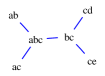
(c) $\mathcal{T}_{2}$, $ab$ and $bc$ joined.

(d) $G_{2}$ $ab$ and $bc$ joined.

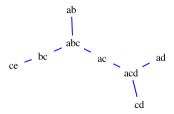
(e) $\mathcal{T}_{2}$ after joining $ac$ and $cd$.

(f) Final $\mathcal{T}_{2}$

Figure 2: Example of graphs during different stages of SearchTree algorithm.

Algorithm 1 SearchTree algorithm. The input is a downward closed cover $\mathcal{F}$, the output is a junction tree $\mathcal{T}$ such that $V\mathopen{}\left(\mathcal{T}\right)\subseteq\mathcal{F}$.

  $V\mathopen{}\left(\mathcal{T}_{0}\right)\leftarrow\left\{x;x\in A\right\}$ {$\mathcal{T}_{0}$ contains the single items.}

  $n\leftarrow 0$.

  repeat

     $n\leftarrow n+1$.

     $\mathcal{T}_{n}\leftarrow\mathcal{T}_{n-1}$.

     $V\mathopen{}\left(G_{n}\right)\leftarrow\left\{X\in V\mathopen{}\left(\mathcal{T}_{n}\right);{\left|X\right|}=n\right\}$.

     $E\mathopen{}\left(G_{n}\right)\leftarrow\left\{\left(X,Y\right);X,Y\in V\mathopen{}\left(G_{n}\right),{\left|X\cap Y\right|}=n-1,X\cup Y\in\mathcal{F}\right\}$.

     repeat

        $e=\left(X,Y\right)\leftarrow\arg\max_{x\in E\mathopen{}\left(G_{n}\right)}w(x)$.

        $E\mathopen{}\left(G_{n}\right)\leftarrow E\mathopen{}\left(G_{n}\right)-e$.

        if $X$ and $Y$ are $n-1$-connected in $\mathcal{T}_{n}$ then

           Call ModifyTree.

        end if

     until $E\mathopen{}\left(G_{n}\right)=\emptyset$

     Delete marked nodes from $\mathcal{T}_{n}$, connect the incident nodes.

  until $G_{n}$ is empty

  return $\mathcal{T}$

Algorithm 2 ModifyTree algorithm.

  $V\leftarrow X\cup Y$.

  $V\mathopen{}\left(\mathcal{T}_{n}\right)\leftarrow V\mathopen{}\left(\mathcal{T}_{n}\right)+V$.

  for $v\in V$ do

     $W\leftarrow V-v$.

     Mark $W$.

     if $W\notin V\mathopen{}\left(G_{n}\right)$ then

        $V\mathopen{}\left(G_{n}\right)\leftarrow V\mathopen{}\left(G_{n}\right)+W$.

        $E\mathopen{}\left(G_{n}\right)\leftarrow E\mathopen{}\left(G_{n}\right)+\left\{\left(W,Z\right);Z\in V\mathopen{}\left(G_{n}\right),{\left|X\cap Z\right|}=n-1,V\neq X\cup Z\in\mathcal{F}\right\}$.

        $V\mathopen{}\left(\mathcal{T}_{n}\right)\leftarrow V\mathopen{}\left(\mathcal{T}_{n}\right)+W$.

     end if

     $E\mathopen{}\left(\mathcal{T}_{n}\right)\leftarrow E\mathopen{}\left(\mathcal{T}_{n}\right)+\left(V,W\right)$.

  end for

  Remove the possible cycle in $\mathcal{T}_{n}$ by removing an edge $\left(U,V\right)$ connecting $X$ and $Y$ and having ${\left|U\cap V\right|}=n-1$.

The next theorem states that the Augment step does not violate the running intersection property.

Theorem 4.1

Let $\mathcal{T}$ be a junction tree with cliques of size $n+1$, at maximum. Let $X,Y\in V\mathopen{}\left(T\right)$ be cliques of size $n$ such that ${\left|X\cap Y\right|}=n-1$. Set $V=X\cup Y$. Then the family $V\mathopen{}\left(\mathcal{T}\right)+V$ is decomposable if and only if $X$ and $Y$ are $n-1$-connected in $\mathcal{T}$.

Theorem 4.2

ModifyTree decreases the entropy of $\mathcal{T}_{n}$ by $w(e)$.

Theorems 4.1–4.2 imply that SearchTree algorithm is nothing more than a greedy search. However, since we are adding cliques in rounds we can state that under some conditions the algorithm returns an optimal cover for each round.

Theorem 4.3

If all the members of $\mathcal{F}$ of size $n+1$ are added to $G_{n}$ at the beginning of the $n$th round, then $\mathcal{T}_{n+1}$ has the lowest entropy among the families refined by $\mathcal{T}_{n}$ and containing the sets of size $n+1$, at maximum.

Corollary 1

The tree $\mathcal{T}_{1}$ is optimal among the families using the sets of size $2$.

Corollary 1 states that $\mathcal{G}_{1}$ is the Chow-Liu tree [10].

4.2 Model Selection

Theorem 1 reveals a drawback in the current approach. Consider that we have two independent items $a$ and $b$ and that $\mathcal{F}=\left\{a,b,ab\right\}$. Note that $\mathcal{F}$ is itself decomposable and $\mathcal{G}=\mathcal{F}$. However, a more reasonable family would be $\left\{a,b\right\}$. To remedy this problem we will use model selection techniques such as BIC [11], AIC [12], and Refined MDL [13]. All these methods score the model by adding a penalty term to the likelihood.

We modify the algorithm by considering only the edges in $G_{n}$ that improve the score. For BIC this reduces to considering only the edges satisfying

$${\left|D\right|}w(e)\geq 2^{n-2}\log{\left|D\right|},$$

where $n$ is the current level of SearchTree algorithm. Using AIC leads to the considering only the edges for which

$${\left|D\right|}w(e)\geq 2^{n-1}.$$

Refined MDL is more troublesome. The penalty term in MDL is known as stochastic complexity. In general, there is no known closed formula for the stochastic complexity, but it can be computed for the multinomial distribution in linear time [14]. However, it is numerically unstable for data with large number of transactions. Hence, we will apply often-used asympotic estimate [15] and define the penalty term

$$C_{\text{MDL}}\mathopen{}\left(k\right)=\frac{k-1}{2}\log{\left|D\right|}-\frac{1}{2}\log\pi-\log\mathrm{\Gamma}\left(k/2\right)$$

for $k$-multinomial distribution.

There are no known exact or approximative solution in a closed form of stochastic complexity for junction trees. Hence we propose the penalty term for the tree to be

$$\sum_{X\in V\mathopen{}\left(\mathcal{T}\right)}C_{\text{MDL}}\mathopen{}\left(2^{{\left|X\right|}}\right)-\sum_{Y\in S\mathopen{}\left(\mathcal{T}\right)}C_{\text{MDL}}\mathopen{}\left(2^{{\left|Y\right|}}\right).$$

Here we think that a single clique $X$ is a $2^{{\left|X\right|}}$-multinomial distribution and we compensate the possible overlaps of the cliques by subtracting the complexity of the separators. Using this estimate leads to a selection criteria

$${\left|D\right|}w(e)\geq C_{\text{MDL}}\mathopen{}\left(2^{{\left|n+1\right|}}\right)-2C_{\text{MDL}}\mathopen{}\left(2^{{\left|n\right|}}\right)+C_{\text{MDL}}\mathopen{}\left(2^{{\left|n-1\right|}}\right).$$

4.3 Computing Multiple Decomposable Families

We can use SearchTree algorithm for computing multiple decomposable covers from a single candidate set $\mathcal{F}$. The motivation behind this approach is that we are able to use more itemsets. We will show empirically in Section 6.4 that the bounds for boolean queries (see Section 5) improve significantly if we are using multiple covers.

Set $\mathcal{F}_{1}=\mathcal{F}$ and let $\mathcal{G}_{1}$ be the first decomposable family constructed from $\mathcal{F}_{1}$ using SearchTree algorithm. We define

$$\mathcal{F}_{2}=\mathcal{F}_{1}-\left\{X\in\mathcal{F}_{1};\text{ there is }Y\in\mathcal{G}_{1},{\left|Y\right|}>1,Y\subseteq X\right\}.$$

We compute $\mathcal{G}_{2}$ from $\mathcal{F}_{2}$ and continue in the iterative fashion until $\mathcal{G}_{k}$ contains nothing but individual items.

5 Boolean Queries with Decomposable Families

One of our motivations for constructing decomposable families is that some computational problems that are hard for general families of itemsets reduce to tractable if the underlying family is decomposable. In this section we will show that the computational burden of a boolean query, a classic optimization problem [16, 17], reduces significantly, if we are using decomposable families of itemsets.

Assume that we are given a set of known itemsets $\mathcal{G}$ and a query itemset $Q\notin\mathcal{G}$. We wish to find $fr\mathopen{}\left(Q;\mathcal{G}\right)$, the possible frequencies for $Q$ given the frequencies of $\mathcal{G}$. It is easy to see that the frequencies form an interval, hence it is sufficient to find the maximal and the minimal frequencies. We can express the problem of finding the maximal frequency as a search for the distribution $p$ solving

$$\begin{array}[]{rl}\max&p\left(Q=1\right)\\ \text{s.t.}&p\left(X=1\right)=fr\mathopen{}\left(X\right),\text{ for each }X\in\mathcal{G}.\\ &p\text{ is a distribution over }A.\end{array}$$ (3)

We can solve Eq. 3 using Linear Programming [16]. However, the number of variables in the program is $2^{{\left|A\right|}}$ and makes the program tractable only for small datasets. In fact, solving Eq. 3 is an NP-hard problem [9].

In the rest of the section we present a method of solving Eq. 3 with a linear program containing only $2^{{\left|Q\right|}}{\left|\mathcal{G}\right|}{\left|A\right|}$ variables, assuming that $\mathcal{G}$ is decomposable. This method is an explicit construction of the technique presented in [18]. The idea behind the approach is that instead of solving a joint distribution in Eq. 3, we break the distribution into small component distributions, one for each clique in the junction tree. These components are forced to be consistent by requiring that they are equal at the separators. The details are given in Algorithm 3.

  $\left\{\mathcal{T}_{1},\ldots,\mathcal{T}_{M}\right\}\leftarrow$ connected components of a junction tree of $\mathcal{G}$.

  for $i=1,\ldots,M$ do

     $Q_{i}\leftarrow Q\cap\left(\bigcup V\mathopen{}\left(\mathcal{T}_{i}\right)\right)$. {Items of $Q$ contained in $\mathcal{T}_{i}$.}

     $\mathcal{U}\leftarrow\arg\min_{\mathcal{S}\subseteq\mathcal{T}_{i}}\left\{{\left|V\mathopen{}\left(\mathcal{S}\right)\right|};Q_{i}\subseteq\bigcup V\mathopen{}\left(\mathcal{S}\right)\right\}$. {Smallest subtree containing $Q_{i}$.}

     while there are changes do

        Remove the items outside $Q_{i}$ that occur in only one clique of $\mathcal{U}$.

        Remove redundant cliques.

     end while

     Select one clique, say $R$ from $\mathcal{U}$ to be the root.

     $R\leftarrow R\cup Q_{i}$. {Augment the root with $Q_{i}$}

     Augment the rest cliques in $\mathcal{U}$ so that the running intersection property holds.

     Let $p_{C}$ be a distribution over each clique $C\in V\mathopen{}\left(\mathcal{U}\right)$.

     $\alpha_{i}\leftarrow$ the solution of a linear program

$$\begin{array}[]{rl}\min&p_{R}\left(Q_{i}=1\right)\\ \text{s.t.}&p_{C}\left(X=1\right)=fr\mathopen{}\left(X\right),\text{ for each }C\in V\mathopen{}\left(\mathcal{U}\right),X\in\mathcal{G},X\subseteq C.\\ &p_{C_{1}}\left(C_{1}\cap C_{2}\right)=p_{C_{2}}\left(C_{1}\cap C_{2}\right),\text{ for each }\left(C_{1},C_{2}\right)\in E\mathopen{}\left(\mathcal{U}\right).\\ \end{array}$$

     $\beta_{i}\leftarrow$ the solution of the maximum version of the linear program.

  end for

  $fr\mathopen{}\left(Q;\mathcal{G}\right)\leftarrow\left[\max\left(\sum_{i}^{M}\alpha_{i}-(M-1),\,0\right),\min_{i}\left(\beta_{i}\right)\right]$.

Algorithm 3 QueryTree algorithm for solving a query $Q$ from a decomposable cover $\mathcal{G}$. The output is the interval $fr\mathopen{}\left(Q;\mathcal{G}\right)$.

To clarify the process we provide the following simple example.

Example 2

Assume that we have $\mathcal{G}$ whose junction tree is given in Figure 3(a). Let query be $Q=adg$. We begin first by finding the smallest sub-tree containing $Q$. This results in purging $fh$ (Figure 3(b)). We further purge the tree by removing $e$ since it only occurs in one clique (Figure 3(c)). In the next step we pick a root, which in this case is $bc$ and augment the cliques with the members of $Q$ so that the root contains $Q$ (Figure 3(d)). We finally remove the redundant cliques which are $ab$, $cd$, $fg$. The final tree is given in 3(e). Finally, the linear program is formed using two distributions $p_{abcdg}$ and $p_{cfg}$. The number of variables in this program is $2^{5}+2^{3}=40$ opposed to the original $2^{8}=256$.

(a) Original $\mathcal{T}$

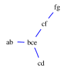
(b) $\mathcal{U}$

(c) Purged $\mathcal{U}$

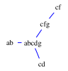
(d) Augmented $\mathcal{U}$

(e) Final $\mathcal{U}$

Figure 3: Junction trees during different stages of solving the query problem.

Note that we did not specify in Algorithm 3 which clique we selected to be the root $R$. The linear program depends on the root $R$ and hence we select the root minimizing the number of variables in the linear program.

Theorem 5.1

QueryTree algorithm solves correctly the boolean query $fr\mathopen{}\left(q;\mathcal{G}\right)$. The number of variables occurring in the linear programs is $2^{{\left|Q\right|}}{\left|\mathcal{G}\right|}{\left|A\right|}$, at maximum.

6 Experiments

In this section we will study empirically the relationship between the decomposable itemset families and the candidate set, the role of the regularization, and the performance of boolean queries using multiple decomposable families.

6.1 Datasets

For our experiments we used one synthetic generated dataset, Path, and three real-world datasets: Paleo, Courses and Mammals. The synthetic dataset, Path, contained 8 items and 100 transactions. Each item was generated from the previous item by flipping it with a $0.3$ probability. The first item was generated by a fair coin flip. The dataset Paleo contains information of mammal fossils found in specific paleontological sites in Europe [19]. Courses describes computer science courses taken by students at the Department of Computer Science of the University of Helsinki. The Mammals dataset consists of presence/absence records of current day European mammals [20]. The basic characteristics of the real-world data sets are shown in Table 1.

Dataset	# of rows	# of items	# of 1s	$\frac{\text{\# of 1s}}{\text{\# of rows}}$
Paleo	501	139	1980	16.0
Courses	3506	98	16086	4.6
Mammals	2183	124	54155	24.8

Table 1: The basic properties of the datasets.

6.2 Generating Decomposable Families

In our first experiment we examined the junction trees that were constructed for the Path dataset. We calculated a sequence of trees using the technique described in Section 4.3. As input to the algorithm we used an unconstrained candidate collection of itemsets (minimum support = 0) from Path and BIC as the regularization method. In Figure 4(a) we see that the first tree corresponds to the model used to generate the dataset. The second tree, given in Figure 4(b), tend to link the items that are one gap away from each other. This is a natural result since close items are the most informative about each other.

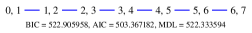
(a) First junction tree of Path data.

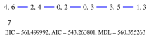
(b) Second junction tree of Path data.

Figure 4: Junction trees for Path, a syntetic data in which an item is generated from the previous item by flipping it with $0.3$ probability. The junction trees are regularized using BIC. The tree in Figure 4(b) is generated by ignoring the cliques of the tree in Figure 4(a).

With Courses data one large junction tree of itemsets is produced with several noticeable components. One distinct component at one end of the tree contains introductory courses like Introduction to Programming, Introduction to Databases, Introduction to Application design and Java Programming. Respectively, the other end of the tree features several distinct components with itemsets on more specialized themes in computer science and software engineering. The central node connecting each of these components in the entire tree is the itemset node {Software Engineering, Models of Programming and Computing, Concurrent systems}.

Figure 5 shows about two-thirds of the entire Courses junction tree, with the component related to introductory courses removed because of the space constraints. We see a concurrent and distributed systems related component in the lower left part of the figure, a more software development oriented component in the lower right quarter and a Robotics/AI component in the upper right corner of the tree. The entire Courses junction tree can be found from [6].

Figure 5: A part of the junction tree constructed from the Courses dataset. The tree was constructed using an unconstrained candidate family (min. support = 0) as input and BIC as regularization.

We continued our experiments by studying the behavior of the model scores in a sequence of trees induced by a corresponding sequence of decomposable families. For the Path data the scores of the two first junction trees are shown in Figure 4, with the first one yielding smaller values. For the real-world datasets, we computed a sequence of trees from each dataset, again, with the unconstrained candidate collection as input and using AIC, BIC, or MDL respectively as the regularization method. Computation took about 1 minute per tree. The corresponding scores are plotted as a function of the order of the corresponding junction tree (Figure 6). The scores are increasing in the sequence, which is expected since the algorithm tries to select the best model and the subsequent trees are constructed from the left-over itemsets. The increase rate slows down towards the end since the last trees tend to have only singleton itemsets as nodes.

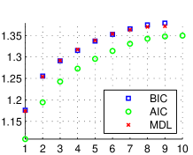
(a) Paleo

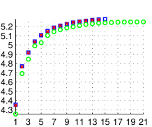
(b) Courses

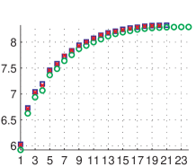
(c) Mammals

Figure 6: Scores of covers as a function of the order of the cover. Each cover is computed with an unconstrained candidate family (min. support = 0) as input and the corresponding regularization. The $y$-axis is the model score divided by $10^{4}$.

6.3 Reducing itemsets

Our next goal was to study the sizes of the generated decomposable families compared to the size of the original candidate set. As input for this experiment, we used several different candidate collections of frequent itemsets resulting from varying the support threshold, and generated the corresponding decomposable itemset families (Table 2).

			First Family, ${\left|\mathcal{G}_{1}\right|}$				All Families, ${\left|\bigcup\mathcal{G}_{i}\right|}$
Dataset	$\sigma$	${\left|\mathcal{F}\right|}$	AIC	BIC	MDL	None	AIC	BIC	MDL	None
Mammals	$.20$	$2169705$	$221$	$213$	$215$	$10663$	$668$	$625$	$630$	$11103$
Mammals	$.25$	$416939$	$201$	$197$	$197$	$6820$	$535$	$507$	$509$	$7106$
Paleo	$.01$	$22283$	$339$	$281$	$290$	$5260$	$993$	$834$	$812$	$6667$
Paleo	$.02$	$979$	$254$	$235$	$239$	$376$	$463$	$433$	$429$	$733$
Paleo	$.03$	$298$	$191$	$190$	$190$	$210$	$231$	$228$	$228$	$277$
Paleo	$.05$	$157$	$147$	$147$	$147$	$151$	$149$	$149$	$149$	$156$
Courses	$.01$	$16945$	$217$	$202$	$206$	$4087$	$565$	$522$	$524$	$4357$
Courses	$.02$	$2493$	$185$	$177$	$177$	$625$	$354$	$342$	$342$	$751$
Courses	$.03$	$773$	$176$	$170$	$170$	$276$	$264$	$261$	$261$	$359$
Courses	$.05$	$230$	$136$	$132$	$132$	$158$	$167$	$164$	$164$	$186$

Table 2: Sizes of decomposable families for various datasets. The second column is the minimum support threshold, the third column is the number of the frequent itemsets in the candidate set. The columns 4–7 contain the size of the first result family and the columns 8–11 contain the size of the union of the result families.

From the results we see that the decomposable families are much smaller compared to the original candidate set, as a large portion of itemsets are pruned due to the running intersection property. The regularizations AIC, BIC, MDL prune the results further. The pruning is most effective when the candidate set is large.

6.4 Boolean Queries

We conducted a series of boolean queries for Paleo and Courses datasets. For each dataset we pick randomly $1000$ queries of size $5$. We constructed a sequence of trees using BIC and the unconstrained (min. support = 0) candidate set as input. The average computation time for a single query was $0.3s$. A portion (abt. 10%) of queries had to be discarded due to the numerical instability of the linear program solver we used.

A query $Q$ for a decomposible family $\mathcal{G}_{i}$ produces a frequency interval $fr\mathopen{}\left(Q;\mathcal{G}_{i}\right)$. We also computed the frequency interval $fr\mathopen{}\left(Q;\mathcal{I}\right)$, where $\mathcal{I}$ is a family containing nothing but singletons. We studied the ratios $r(Q;n)={\left|\bigcap_{1}^{n}fr\mathopen{}\left(Q;\mathcal{G}_{i}\right)\right|}/{\left|fr\mathopen{}\left(Q;\mathcal{I}\right)\right|}$ as a function of $n$, that is, the ratio between the tightness of the bound using $n$ families and the singleton model.

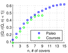
(a) Improved queries

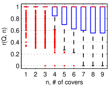
(b) Paleo

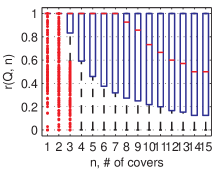
(c) Courses

Figure 7: Boolean query ratios from Paleo and Course datasets. Figure 7(a) contains the percentage of queries having $r(Q;n)<1$, that is, the percentage of queries improved over the singleton model as a function of the number of decomposable families. Figures 7(b)–7(c) are box plots of the ratios $r(Q;n)$, where $Q$ is a random query and $n$ is the number of decomposable families.

From the results given in Figure 7 we see that the first decomposible family in the sequence yields in about 10 % of the queries an improved bound with respect to the singleton family. As the number of decomposable families increases, the number of queries with tighter bounds goes from $10\%$ up to $60\%$. Also, in general the absolute bounds become tighter for the queries as we increase the number of decomposable families. For Courses the median of the ratio $r(Q;15)$ is about $0.5$.

7 Related Work

One of the main uses of our algorithm is in reducing itemset mining results into a smaller and a more manageable group of itemsets. One of the earliest approaches on itemset reduction include close itemsets [21] and maximal frequent itemset [22]. Also more recently, a significant amount of interesting research has been produced on the topic [23, 24, 25, 26]. Yan et al. [24] proposed a statistical model in which $k$ representative patterns are used to summarize the original itemset family as well as possible. This approach has, however, a different goal to that of ours, as our model aims to describe the data itself. From this point of view the work by Siebes et al. [25] is perhaps the most in concordance to ours. Siebes et al. propose an MDL based method where the reduced group of itemsets aim to compress the data as well as possible. Yet, their approach is technically and methodologically quite different and does not provide a probabilistic model of the data as our model does. Furthermore, non of the above approaches provide a naturally following tree based representation of the mining results as our model does.

Traditionally, junction trees are not used as a direct model but rather as a technique for decomposing directed acyclic graph (DAG) models [5]. However, there is a clear difference between the DAG models and our approach. Assume that we have 4 items $a$, $b$, $c$, and $d$. Consider a DAG model $p(a)p(b;a)p(c;a)p(d;bc)$. While we can decompose this model using junction trees we cannot express it exactly. The reason for this is that the DAG model contains the assumption of independence of $b$ and $c$ given $a$. This allows us to break the clique $abc$ into smaller parts. In our approach the cliques are the empirical distributions with no independence assumptions. DAG models and junction tree models are equivalent for Chow-Liu tree models [10].

Our algorithm for constructing junction trees is closely related to EFS algorithm [27, 28] in which new cliques are created in a similar fashion. The main difference between the approaches is that we add new cliques in a level-wise fashion. This allows a more straightforward algorithm. Another benefit of our approach is Theorem 4.3. On the other hand, Corollary 1 implies that our algorithm can be seen also as an extension of Chow-Liu tree model [10].

8 Conclusions and Future Work

In this study we applied the concept of junction trees to create decomposable families of itemsets. The approach suits well for the problem of itemset selection, and has several advantages. The naturally following junction trees provide an intuitive representation of the mining results. From the computational point of view, the model provides leverage for problems that could be intractable using generic families of itemsets. We provided an efficient algorithm to build decomposable itemset families, and gave an application example with frequency bound querying using the model. Empirical results showed that our algorithm yields high quality results. Because of the expressiveness and good interpretability of the model, applications such as classification using decomposable families of itemsets could prove an interesting avenue for future research. Even more generally, we anticipate that in the future decomposable models could prove computationally useful with pattern mining applications that otherwise could be hard to tackle.

Appendix 0.A Appendix

Proof of Theorem 4.1

The theorem is trivial for the case $n=1$. Hence we assume that $n>1$.

Assume that $X$ and $Y$ are $n-1$-connected in $\mathcal{T}$, and let $P$ be the path connecting $X$ and $Y$. If $\left(X,Y\right)\notin P$ , then there exists $f=\left(Z,W\right)\in P$ such that ${\left|Z\cap W\right|}=n-1$. Since $\mathcal{T}$ is a junction tree, we must have $Z\cap W=X\cap Y$. Hence by removing $f$ and adding $\left(X,Y\right)$ does not violate the running intersection property. Thus we can assume that $\left(X,Y\right)\in E\mathopen{}\left(\mathcal{T}\right)$. Adding $V$ between $X$ and $Y$ does not violate the running intersection property and hence $V\mathopen{}\left(\mathcal{T}\right)+V$ remains decomposable.

To prove the other direction assume that $X$ and $Y$ are not $n-1$ connected. This implies that the path $P$ from $X$ to $Y$ consists of $n+1$ cliques with $n$ separators. Assume that $V\mathopen{}\left(\mathcal{T}\right)+V$ is decomposable and hence there is a juncion tree $\mathcal{U}$ having $V\mathopen{}\left(\mathcal{U}\right)=V\mathopen{}\left(\mathcal{T}\right)+V$. We can modify $\mathcal{U}$ such that the edges of the path $P$ occur in $\mathcal{U}$. Let $P_{s}$ be the first clique in $P$ and let $P_{l}$ be the last. Note that $V\subset P_{s}\cup P_{l}$. Let $P_{e}$ be the first clique in $P$ along the path from $V$ to $P_{s}$. Since ${\left|P_{s}\cap V\right|}=n$, we must have $P_{e}\cap V=P_{s}\cap V$ The path from $V$ to $P_{l}$ must also go through $P_{e}$, hence we must have $P_{s}\cap V=P_{l}\cap V$. This implies that either $V=P_{s}$ or $V=P_{l}$, which is a contradiction. This completes the proof.

Proof of Theorem 4.2

Assume that the edge $e=\left(X,Y\right)\in E\mathopen{}\left(\mathcal{T}_{n}\right)$. Let $\mathcal{T}^{\prime}_{n}$ be the tree after adding $X\cup Y$. The entropy of the original tree is

$$H\mathopen{}\left(\mathcal{T}_{n}\right)=H\mathopen{}\left(X\right)+H\mathopen{}\left(Y\right)-H\mathopen{}\left(X\cap Y\right)+B,$$

where $B$ is the impact of the rest nodes. The entropy of the new tree is

$$H\mathopen{}\left(\mathcal{T}^{\prime}_{n}\right)=H\mathopen{}\left(X\cup Y\right)+B.$$

Hence we have $H\mathopen{}\left(\mathcal{T}_{n}\right)-H\mathopen{}\left(\mathcal{T}^{\prime}_{n}\right)=w(e)$.

Proof of Theorem 4.3

It is easy to see that the cliques $X$ and $Y$ are $n-1$ -connected if and only if they are not connected by the previous edges from $G_{n}$. Hence, the algorithm reduces to Kruskal’s algorithm in finding the optimal spanning tree of $G_{n}$, thus returning the optimal spanning tree.

Let $\mathcal{U}$ be a junction tree refined by $\mathcal{T}_{n}$ and containing the cliques of size $n+1$, at maximum. The cliques of size $n+1$ occur in $G_{n}$. Let $H$ be the corresponding edges in $G_{n}$. To prove the theorem we need to show that $H$ contains no cycles.

Assume othewise, and consider adding the edges in $H$, one at the time. When the first cycle occurs, the corresponding family is not decomposable by Theorem 4.1. The argument in the proof of Theorem 4.1 holds even if we keep adding cliques of size $n+1$, hence the final family cannot be decomposable. Thus $H$ cannot contain cycles.

Proof of Theorem 5.1

Theorem 6 in [dobra00bounds] guarantees that breaking $\mathcal{G}$ into connected components and computing $fr\mathopen{}\left(Q;\mathcal{G}\right)$ from $\alpha_{i}$ and $\beta_{i}$ produce an accurate result as long as $\alpha_{i}$ and $\beta_{i}$ are accurate. Theorem 7 in [18] states that taking the smallest subtree containing $Q_{i}$ and removing attributes occuring in only one clique does not change $\alpha_{i}$ and $\beta_{i}$.

Finally, we need to prove that the linear program of the algorithm produce the same $\alpha_{i},\beta_{i}$ as the linear program in Eq. 3. Let $p$ be a distribution satisfying the conditions in Eq. 3. Clearly, we can break $p$ into components satisfying the conditions of the linear program given in the algorithm. On other hand, assume that $\left\{p_{C}\right\}$ now satisfy the conditions of the linear program given in the algorithm. Since components are equal at the separators we can combine this into one joint distribution $p$ satisfying the condition of Eq. 3. This implies that the outcome of both programs are equivalent.

To prove the bound for the number of variables, note that for any clique $C$ we have $2^{{\left|C\right|}}\leq{\left|\mathcal{G}\right|}$. We can have ${\left|A\right|}$ cliques at most. Augmenting can increase the size of the cliques by ${\left|Q\right|}$, at maximum. This implies that the number of variables is $\sum_{i}2^{{\left|Q\right|}+{\left|C_{i}\right|}}=2^{{\left|Q\right|}}\sum_{i}2^{{\left|C_{i}\right|}}\leq 2^{{\left|Q\right|}}{\left|\mathcal{G}\right|}{\left|A\right|}$.

Figure 8: Junction tree build from the Courses dataset. The tree was constructed using an unconstrained candidate family (min. support = 0) as input and BIC as regularization.

References

- [1] Agrawal, R., Imielinski, T., Swami, A.: Mining association rules between sets of items in large databases. In: ACM SIGMOD international conference on Management of data. (1993) 207–216
- [2] Agrawal, R., Mannila, H., Srikant, R., Toivonen, H., Verkamo, A.: Fast discovery of association rules. Advances in knowledge discovery and data mining (1996) 307–328
- [3] Han, J., Pei, J.: Mining frequent patterns by pattern-growth: methodology and implications. SIGKDD Explorations Newsletter 2(2) (2000) 14–20
- [4] Han, J., Cheng, H., Xin, D., Yan, X.: Frequent pattern mining: current status and future directions. Data Mining and Knowledge Discovery 15(1) (2007)
- [5] Cowell, R.G., Dawid, A.P., Lauritzen, S.L., Spiegelhalter, D.J.: Probabilistic Networks and Expert Systems. Statistics for Engineering and Information Science. Springer-Verlag (1999)
- [6] Tatti, N., Heikinheimo, H.: Decomposable families of itemsets. Technical Report TKK-ICS-R1, Helsinki University of Technology (2008) http://www.cis.hut.fi/ntatti/tatti08decomposable.pdf.
- [7] Jiroušek, R., Přeušil, S.: On the effective implementation of the iterative proportional fitting procedure. Computational Statistics and Data Analysis 19 (1995) 177–189
- [8] Csiszár, I.: I-divergence geometry of probability distributions and minimization problems. The Annals of Probability 3(1) (Feb. 1975) 146–158
- [9] Tatti, N.: Computational complexity of queries based on itemsets. Information Processing Letters (June 2006) 183–187
- [10] Chow, C.K., Liu, C.N.: Approximating discrete probability distributions with dependence trees. IEEE Transactions on Information Theory 14(3) (May 1968) 462–467
- [11] Schwarz, G.: Estimating the dimension of a model. Annals of Statistics 6(2) (1978) 461–464
- [12] Akaike, H.: A new look at the statistical model identification. IEEE Transactions on Automatic Control 19(6) (1974) 716–723
- [13] Grünwald, P.D.: The Minimum Description Length Principle (Adaptive Computation and Machine Learning). The MIT Press (2007)
- [14] Kontkanen, P., Myllymäki, P.: A linear-time algorithm for computing the multinomial stochastic complexity. Information Processing Letters 103(6) (2007) 227–233
- [15] Rissanen, J.: Fisher information and stochastic complexity. IEEE Transactions on Information Theory 42(1) (1996) 40–47
- [16] Hailperin, T.: Best possible inequalities for the probability of a logical function of events. The American Mathematical Monthly 72(4) (Apr. 1965) 343–359
- [17] Bykowski, A., Seppänen, J.K., Hollmén, J.: Model-independent bounding of the supports of Boolean formulae in binary data. In Lanzi, P.L., Meo, R., eds.: Database Support for Data Mining Applications: Discovering Knowledge with Inductive Queries. LNCS 2682, Springer Verlag (2004) 234–249
- [18] Tatti, N.: Safe projections of binary data sets. Acta Informatica 42(8–9) (April 2006) 617–638
- [19] Fortelius, M.: Neogene of the old world database of fossil mammals (NOW). University of Helsinki, http://www.helsinki.fi/science/now/ (2005)
- [20] Mitchell-Jones, A.J., Amori, G., Bogdanowicz, W., Krystufek, B., Reijnders, P.J.H., Spitzenberger, F., Stubbe, M., Thissen, J.B.M., Vohralik, V., Zima, J.: The Atlas of European Mammals. Academic Press (1999)
- [21] Pasquier, N., Bastide, Y., Taouil, R., Lakhal, L.: Discovering frequent closed itemsets for association rules. Lecture Notes in Computer Science 1540 (1999) 398–416
- [22] Roberto J. Bayardo, J.: Efficiently mining long patterns from databases. In: ACM SIGMOD international conference on Management of data, New York, NY, USA, ACM (1998) 85–93
- [23] Calders, T., Goethals, B.: Mining all non-derivable frequent itemsets. In: European Conference on Principles and Practice of Knowledge Discovery in Databases. (2002)
- [24] Yan, X., Cheng, H., Han, J., Xin, D.: Summarizing itemset patterns: A profile-based approach. In: ACM SIGKDD international conference on Knowledge Discovery and Data Mining. (2005)
- [25] Siebes, A., Vreeken, J., van Leeuwen, M.: Item sets that compress. In: SIAM Conference on Data Mining. (2006) 393–404
- [26] Bringmann, B., Zimmermann, A.: The chosen few: On identifying valuable patterns. In: IEEE International Conference on Data Mining. (2007)
- [27] Deshpande, A., Garofalakis, M.N., Jordan, M.I.: Efficient stepwise selection in decomposable models. In: Conference in Uncertainty in Artificial Intelligence, San Francisco, CA, USA, Morgan Kaufmann Publishers Inc. (2001) 128–135
- [28] Altmueller, S.M., Haralick, R.M.: Practical aspects of efficient forward selection in decomposable graphical models. In: IEEE International Conference on Tools with Artificial Intelligence, Washington, DC, USA, IEEE Computer Society (2004) 710–715