Model Embedding Model-Based Reinforcement Learning

Xiaoyu Tan 111Equal contribution with randomized order. Ant Financial Services Group Chao Quโˆ— Ant Financial Services Group Junwu Xiong Ant Financial Services Group James Zhang Ant Financial Services Group
Abstract

Model-based reinforcement learning (MBRL) has shown its advantages in sample-efficiency over model-free reinforcement learning (MFRL). Despite the impressive results it achieves, it still faces a trade-off between the ease of data generation and model bias. In this paper, we propose a simple and elegant model-embedding model-based reinforcement learning (MEMB) algorithm in the framework of the probabilistic reinforcement learning. To balance the sample-efficiency and model bias, we exploit both real and imaginary data in the training. In particular, we embed the model in the policy update and learn $Q$ and $V$ functions from the real data set. We provide the theoretical analysis of MEMB with the Lipschitz continuity assumption on the model and policy. At last, we evaluate MEMB on several benchmarks and demonstrate our algorithm can achieve state-of-the-art performance.

1 Introduction

Reinforcement learning can be generally classified into two categories: model-free reinforcement learning (MFRL) and model-based reinforcement learning (MBRL). There is a surge of interest in MBRL recently due to its higher sample-efficiency comparing with MFRL (Kurutach etย al., 2018; Heess etย al., 2015; Asadi etย al., 2018). Despite its success, MBRL still faces a challenging problem, i.e., the model-bias, where the imperfect dynamics model would degrade the performance of the algorithm (Kurutach etย al., 2018). Unfortunately, such things always happen when the environment is sufficiently complex. There are a few efforts to mitigate such issues by combining model-based and model-free approaches. Heess etย al. (2015) compute the value gradient along real system trajectories instead of planned ones to avoid the compounded error. Kalweit and Boedecker (2017) mix the real data and imaginary data from the model and then train $Q$ function. An ensemble of neural networks can be applied to model the environment dynamics, which effectively reduces the error of the model (Kurutach etย al., 2018; Clavera etย al., 2018; Chua etย al., 2018).

Indeed, how to exploit the real and imaginary data is a key question in model-based reinforcement learning. Recent model-based algorithms applying Dyna-style updates have demonstrated promising results (Sutton, 1990; Kurutach etย al., 2018; Luo etย al., 2018). They collect real data using the current policy to train the dynamics model. Then the policy is improved using state-of-the-art model-free reinforcement learning algorithms with imagined data generated by the learned model. Our argument is that why not directly embed the model into the policy improvement? To this end, we derive a reinforcement learning algorithm called model-embedding model-based reinforcement learning (MEMB) in the framework of the probabilistic reinforcement learning (Levine, 2018).

We provide the theoretical result on the error of the long term return in MEMB, which is caused by the model bias and policy distribution shift given the Lipschitz continuity condition of the model and policy. In addition, our analysis takes consideration of the length of the rollout step, which helps us to design the algorithm. In MEMB, the dynamics model and reward model are trained with the real data set collected from the environment. Then we simply train $Q$ and $V$ function using the real data set with the update rule derived from the maximum entropy principle (several other ways to include the imaginary data can also be applied, see discussions in Section 3). In the policy improvement step, the stochastic actor samples an action with the real state as the input, and then the state switches from s๐‘ s to sโ€ฒsuperscript๐‘ โ€ฒs^{\prime} according to the learned dynamics model.

We link the learned dynamics model, reward model, and policy to compute an analytic policy gradient by the back-propagation. Comparing with the likelihood-ratio estimator usually used in the MFRL method, such value gradient method would reduce the variance of the policy gradient (Heess etย al., 2015). The other merit of MEMB is its computational efficiency. Several state-of-the-art MBRL algorithms generate hundreds of thousands imaginary data from the model and a few real samples (Luo etย al., 2018; Janner etย al., 2019). Then the huge imaginary data set feeds into MFRL algorithms, which may be sample-efficient in terms of real samples but not computational-friendly. On the contrary, our algorithm embeds the model in the policy update. Thus we can implement it efficiently by computing policy gradient several times in each iteration (see our algorithm 1) and do not need to do the calculation on the huge imaginary data set.

Notice SVG (Heess etย al., 2015) also embeds the model to compute the policy gradient. However, there are several key differences between MEMB and SVG.

  • โ€ข

    To alleviate the issue of the compounded error, SVG proposes a conservative algorithm where just real data is used to evaluate policy gradients and the imaginary data is wasted. However, our theorem shows that the imaginary data from the short rollout from the learned model can be trusted. In our work, the policy is trained with the model and imaginary dataset $m$ times in each iteration of the algorithm. In the ablation study (appendix B), we demonstrate such difference leads to a large gap in the performance.

  • โ€ข

    We provide a theoretical guarantee of the algorithm, which is not included in SVG.

  • โ€ข

    We derive our algorithm in the framework of the probabilistic reinforcement learning. The entropy term would encourage the exploration, prevent the early convergence to the sub-optimal policies, and show state-of-the-art performance in MFRL (Haarnoja etย al., 2018).

In addition, MEMB avoids the importance sampling in the off-policy setting by sampling the action from $\pi$ and transition from the learned model, which further reduces the variance of the gradient estimation.

Contributions: We derive an elegant, sample-efficient, and computational-friendly 222We can finish one trial of the experiment around one or two hours on a laptop. Dyna-style MBRL algorithm in the framework of the probabilistic reinforcement learning in a principled way. Different from the traditional MBRL algorithm, we directly embed the model into the policy improvement, which could reduce the variance in the gradient estimation and avoid the computation on the huge imaginary data set. In addition, since the algorithm is off-policy, it is sample-efficient. At last, we provide theoretical results of our algorithm on the long term return considering the model bias and policy distribution shift. We test our algorithm on several benchmark tasks in Mujoco simulation environment (Todorov etย al., 2012) and demonstrate that our algorithm can achieve state-of-the-art performance. We provide our code anonymously for the reproducibility 333Code is submitted at https://github.com/MEMB-anonymous1/MEMB .

Related work: There are a plethora of works on MBRL. They can be classified into several categories depending on the way to utilize the model, to search the optimal policy or the function approximator of the dynamics model. We leave the comprehensive discussion on the related work in appendix A.

2 Preliminaries

In this section, we first present some backgrounds on the Markov decision process. Then we introduce the knowledge on the probabilistic reinforcement learning with entropy regularization (Ziebart etย al., 2008; Levine, 2018) and stochastic value gradient (Heess etย al., 2015) since parts of them are the building blocks of our algorithm.

2.1 MDP

Markov Decision Process (MDP) can be described by a 5-tuple ($\mathcal{S},\mathcal{A},r,p,\gamma$): $\mathcal{S}$ is the state space, $\mathcal{A}$ is the action space, $p$ is the transition probability, $r$ is the expected reward, and $\gamma\in[0,1)$ is the discount factor. That is for sโˆˆ๐’ฎ๐‘ ๐’ฎs\in\mathcal{S} and $a\in\mathcal{A}$, rโ€‹(s,a)๐‘Ÿ๐‘ ๐‘Žr(s,a) is the expected reward, pโ€‹(sโ€ฒ|s,a)๐‘conditionalsuperscript๐‘ โ€ฒ๐‘ ๐‘Žp(s^{\prime}|s,a) is the probability to reach the state sโ€ฒsuperscript๐‘ โ€ฒs^{\prime}. A policy is used to select actions in the MDP. In general, the policy is stochastic and denoted by $\pi$, where ฯ€โ€‹(at|st)๐œ‹conditionalsubscript๐‘Ž๐‘กsubscript๐‘ ๐‘ก\pi(a_{t}|s_{t}) is the conditional probability density at $a_{t}$ associated with the policy. The state value evaluated on policy $\pi$ could be represented by Vฯ€โ€‹(s)=๐”ผฯ€โ€‹[โˆ‘t=0โˆžฮณtโ€‹rโ€‹(st,at)|s0=s]superscript๐‘‰๐œ‹๐‘ subscript๐”ผ๐œ‹delimited-[]conditionalsuperscriptsubscript๐‘ก0superscript๐›พ๐‘ก๐‘Ÿsubscript๐‘ ๐‘กsubscript๐‘Ž๐‘กsubscript๐‘ 0๐‘ V^{\pi}(s)=\mathbb{E}_{\pi}[\sum_{t=0}^{\infty}\gamma^{t}r(s_{t},a_{t})|s_{0}=s] on immediate reward return $r$ with discount factor $\gamma\in(0,1)$ along the horizon $t$. When the entropy of the policy is incorporated in the probabilistic reinforcement learning (Ziebart etย al., 2008), we could redefine the reward function rโ€‹(s,a)โ†rโ€‹(s,a)โˆ’logโกฯ€โ€‹(a|s)โ†๐‘Ÿ๐‘ ๐‘Ž๐‘Ÿ๐‘ ๐‘Ž๐œ‹conditional๐‘Ž๐‘ r(s,a)\leftarrow r(s,a)-\log\pi(a|s). When the model of the environment is learned from the data, we use p^โ€‹(sโ€ฒ|s,a)^๐‘conditionalsuperscript๐‘ โ€ฒ๐‘ ๐‘Ž\hat{p}(s^{\prime}|s,a) to denote the learned dynamic model, and r^โ€‹(s,a)^๐‘Ÿ๐‘ ๐‘Ž\hat{r}(s,a) as the learned reward model.

We denote the true long term return as ฮทโ€‹(ฯ€):=๐”ผฯ€โ€‹โˆ‘t=0โˆžฮณtโ€‹rโ€‹(st,at)assign๐œ‚๐œ‹subscript๐”ผ๐œ‹superscriptsubscript๐‘ก0superscript๐›พ๐‘ก๐‘Ÿsubscript๐‘ ๐‘กsubscript๐‘Ž๐‘ก\eta(\pi):=\mathbb{E}_{\pi}\sum_{t=0}^{\infty}\gamma^{t}r(s_{t},a_{t}), where the expectation corresponds to the policy, true transition and true reward. In the model based reinforcement learning, we denote the model long term return as ฮท^โ€‹(ฯ€):=๐”ผ^ฯ€โ€‹โˆ‘t=0โˆžฮณtโ€‹r^โ€‹(st,at)assign^๐œ‚๐œ‹subscript^๐”ผ๐œ‹superscriptsubscript๐‘ก0superscript๐›พ๐‘ก^๐‘Ÿsubscript๐‘ ๐‘กsubscript๐‘Ž๐‘ก\hat{\eta}(\pi):=\hat{\mathbb{E}}_{\pi}\sum_{t=0}^{\infty}\gamma^{t}\hat{r}(s_{t},a_{t}), where $\hat{\mathbb{E}}$ means the expectation over the policy, learned model $\hat{p}$ and $\hat{r}$.

2.2 Probabilistic Reinforcement Learning

Levine (2018) formulate reinforcement learning as a probabilistic inference problem. The trajectory $\tau$ up to time step $T$ is defined as

ฯ„=((s0,a0),(s1,a1),โ€ฆ,(sT,aT)).๐œsubscript๐‘ 0subscript๐‘Ž0subscript๐‘ 1subscript๐‘Ž1โ€ฆsubscript๐‘ ๐‘‡subscript๐‘Ž๐‘‡\tau=((s_{0},a_{0}),(s_{1},a_{1}),...,(s_{T},a_{T})).

The probability of the trajectory with the optimal policy is defined as

ฯ=[pโ€‹(s0)โ€‹โˆt=0Tpโ€‹(st+1|st,at)]โ€‹expโก(โˆ‘t=0Trโ€‹(st,at)).๐œŒdelimited-[]๐‘subscript๐‘ 0superscriptsubscriptproduct๐‘ก0๐‘‡๐‘conditionalsubscript๐‘ ๐‘ก1subscript๐‘ ๐‘กsubscript๐‘Ž๐‘กsuperscriptsubscript๐‘ก0๐‘‡๐‘Ÿsubscript๐‘ ๐‘กsubscript๐‘Ž๐‘ก\rho=[p(s_{0})\prod_{t=0}^{T}p(s_{t+1}|s_{t},a_{t})]\exp\big{(}\sum_{t=0}^{T}r(s_{t},a_{t})\big{)}.

The probability of the trajectory induced by the policy ฯ€โ€‹(a|s)๐œ‹conditional๐‘Ž๐‘ \pi(a|s) is

ฯ~=pโ€‹(s0)โ€‹โˆt=0Tpโ€‹(st+1|st,at)โ€‹ฯ€โ€‹(at|st).~๐œŒ๐‘subscript๐‘ 0superscriptsubscriptproduct๐‘ก0๐‘‡๐‘conditionalsubscript๐‘ ๐‘ก1subscript๐‘ ๐‘กsubscript๐‘Ž๐‘ก๐œ‹conditionalsubscript๐‘Ž๐‘กsubscript๐‘ ๐‘ก\tilde{\rho}=p(s_{0})\prod_{t=0}^{T}p(s_{t+1}|s_{t},a_{t})\pi(a_{t}|s_{t}).

The objective is to minimize the KL divergence $KL(\tilde{\rho},\rho)$, which leads to the entropy regularized reinforcement learning $\max_{\pi}\sum_{t=0}^{T}\mathbb{E}_{(s_{t},a_{t})\sim\rho_{\pi}}[r(s_{t},a_{t})+\alpha\mathcal{H}(\pi(\cdot|s_{t}))],$ where $\mathcal{H}(\pi(\cdot|s_{t}))$ is an entropy term scaled by $\alpha$ (Ziebart etย al., 2008). The optimal policy can be obtained by the following soft-Q update (Fox etย al., 2016).

Qโ€‹(st,at)โŸตrโ€‹(st,at)+ฮณโ€‹๐”ผst+1โˆผpโ€‹[Vโ€‹(st+1)],Vโ€‹(st)โ†ฮฑโ€‹logโก(โˆซ๐’œexpโก(1ฮฑโ€‹Qโ€‹(st,at))โ€‹๐‘‘at).formulae-sequenceโŸต๐‘„subscript๐‘ ๐‘กsubscript๐‘Ž๐‘ก๐‘Ÿsubscript๐‘ ๐‘กsubscript๐‘Ž๐‘ก๐›พsubscript๐”ผsimilar-tosubscript๐‘ ๐‘ก1๐‘delimited-[]๐‘‰subscript๐‘ ๐‘ก1โ†๐‘‰subscript๐‘ ๐‘ก๐›ผsubscript๐’œ1๐›ผ๐‘„subscript๐‘ ๐‘กsubscript๐‘Ž๐‘กdifferential-dsubscript๐‘Ž๐‘กQ(s_{t},a_{t})\longleftarrow r(s_{t},a_{t})+\gamma\mathbb{E}_{s_{t+1}\sim p}[V(s_{t+1})],V(s_{t})\leftarrow\alpha\log(\int_{\mathcal{A}}\exp(\frac{1}{\alpha}Q(s_{t},a_{t}))da_{t}).

Above iterations define the soft $Q$ operator, which is a contraction. The optimal policy ฯ€โˆ—โ€‹(a|s)superscript๐œ‹conditional๐‘Ž๐‘ \pi^{*}(a|s) can be recovered by ฯ€โ‹†โ€‹(at|st)=expโก(1ฮฑโ€‹Qโˆ—โ€‹(st,at))โˆซ๐’œexpโก(1ฮฑโ€‹Qโˆ—โ€‹(st,at))โ€‹๐‘‘atsuperscript๐œ‹โ‹†conditionalsubscript๐‘Ž๐‘กsubscript๐‘ ๐‘ก1๐›ผsuperscript๐‘„subscript๐‘ ๐‘กsubscript๐‘Ž๐‘กsubscript๐’œ1๐›ผsuperscript๐‘„subscript๐‘ ๐‘กsubscript๐‘Ž๐‘กdifferential-dsubscript๐‘Ž๐‘ก\pi^{\star}(a_{t}|s_{t})=\frac{\exp(\frac{1}{\alpha}Q^{*}(s_{t},a_{t}))}{\int_{\mathcal{A}}\exp(\frac{1}{\alpha}Q^{*}(s_{t},a_{t}))da_{t}}, where $Q^{*}$ is the fixed point of the soft-Q update. We refer readers to the work (Ziebart etย al., 2008; Haarnoja etย al., 2017) for more discussions. In soft actor-critic (Haarnoja etย al., 2018), the optimal policy ฯ€โˆ—โ€‹(at|st)superscript๐œ‹conditionalsubscript๐‘Ž๐‘กsubscript๐‘ ๐‘ก\pi^{*}(a_{t}|s_{t}) is approximated by a neural network ฯ€ฮธโ€‹(at|st)subscript๐œ‹๐œƒconditionalsubscript๐‘Ž๐‘กsubscript๐‘ ๐‘ก\pi_{\theta}(a_{t}|s_{t}), which is obtained by solving the following optimization problem

$$\max_{\pi_{\theta}(a_{t}|s_{t})}\mathbb{E}_{s_{t}\sim p(s_{t})}\mathbb{E}_{a_{t}\sim\pi_{\theta}(a_{t}|s_{t})}[Q(s_{t},a_{t})-\alpha\log\pi_{\theta}(a_{t}|s_{t}))].$$

2.3 Stochastic Value Gradient

Stochastic value gradient method is a model-based algorithm which is designed to avoid the compounded model errors by only using the real-world observation and gradient information from the model (Heess etย al., 2015). The algorithm directly substitutes the dynamics model and reward model in the Bellman equation and calculates the gradient. To perform the backpropagation in the stochastic Bellman equation, the re-parameterization trick is applied to evaluate the gradient on real-world data. In SVG(1), the stochastic policy ฯ€โ€‹(a|s;ฮธ)๐œ‹conditional๐‘Ž๐‘ ๐œƒ\pi(a|s;\theta) with parameter $\theta$ could be optimized by the policy gradient in the following way

โˆ‚Vโ€‹(s)โˆ‚ฮธโ‰ˆ๐”ผฮท,ฮถโ€‹[โˆ‚r^โ€‹(s,a)โˆ‚aโ€‹โˆ‚ฯ€โ€‹(a|s)โˆ‚ฮธ+ฮณโ€‹(โˆ‚Vโ€ฒโ€‹(sโ€ฒ)โˆ‚sโ€ฒโ€‹โˆ‚fโ€‹(s,a)โˆ‚aโ€‹โˆ‚ฯ€โ€‹(a|s)โˆ‚ฮธ)],๐‘‰๐‘ ๐œƒsubscript๐”ผ๐œ‚๐œdelimited-[]^๐‘Ÿ๐‘ ๐‘Ž๐‘Ž๐œ‹conditional๐‘Ž๐‘ ๐œƒ๐›พsuperscript๐‘‰โ€ฒsuperscript๐‘ โ€ฒsuperscript๐‘ โ€ฒ๐‘“๐‘ ๐‘Ž๐‘Ž๐œ‹conditional๐‘Ž๐‘ ๐œƒ\displaystyle\frac{\partial V(s)}{\partial\theta}\approx\mathbb{E}_{\eta,\zeta}[\frac{\partial\hat{r}(s,a)}{\partial a}\frac{\partial\pi(a|s)}{\partial\theta}+\gamma(\frac{\partial V^{\prime}(s^{\prime})}{\partial s^{\prime}}\frac{\partial f(s,a)}{\partial a}\frac{\partial\pi(a|s)}{\partial\theta})], (1)

where $\eta$ and $\zeta$ are the policy and model re-parameterization noise which could be directly sampled from a prior distribution or inferred from a generative model gโ€‹(ฮท,ฮถ|s,a,sโ€ฒ)๐‘”๐œ‚conditional๐œ๐‘ ๐‘Žsuperscript๐‘ โ€ฒg(\eta,\zeta|s,a,s^{\prime}). The fโ€‹(s,a)๐‘“๐‘ ๐‘Žf(s,a) and r^โ€‹(s,a)^๐‘Ÿ๐‘ ๐‘Ž\hat{r}(s,a) are dynamics model and reward model respectively. In the off-policy update, SVG includes the important weight w=ฯ€โ€‹(ak|sk,ฮธt)ฯ€โ€‹(ak|sk,ฮธk)๐‘ค๐œ‹conditionalsubscript๐‘Ž๐‘˜subscript๐‘ ๐‘˜subscript๐œƒ๐‘ก๐œ‹conditionalsubscript๐‘Ž๐‘˜subscript๐‘ ๐‘˜subscript๐œƒ๐‘˜w=\frac{\pi(a_{k}|s_{k},\theta_{t})}{\pi(a_{k}|s_{k},\theta_{k})}, where $\theta_{t}$ represent the parameter of the current policy and $k$ is the index of the data from the replay buffer.

Notions: Given two metric space $(X,d_{X})$ and $(Y,d_{Y})$, we say a function $f$ is $L$ Lipschitz if $d_{Y}(f(x_{1}),f(x_{2}))\leq Ld_{X}(x_{1},x_{2}),\forall x_{1},x_{2}\in X$. Give a meritc space $(M,d)$ and the set $\mathbb{P}(M)$ of probability measures on $M$, the Wasserstein metric between two probability distributions $\mu_{1}$ and $\mu_{2}$ in $\mathbb{P}(M)$ is defined as $W(\mu_{1},\mu_{2}):=\inf_{j\in\Sigma}\int\int p(x,y)d(x,y)dxdy,$ where $\Sigma$ denotes the collection of all joint distributions $p$ with marginal $\mu_{1}$ and $\mu_{2}$.

3 MEMB

In this section, we introduce our model-embedding model-based reinforcement learning algorithm (MEMB). Particularly, we optimize the following model long term return with the entropy regularization.

maxฯ€โ€‹โˆ‘t=0T๐”ผ^โ€‹[r^โ€‹(st,at)+โ„‹โ€‹(ฯ€โ€‹(at|st))],subscript๐œ‹superscriptsubscript๐‘ก0๐‘‡^๐”ผdelimited-[]^๐‘Ÿsubscript๐‘ ๐‘กsubscript๐‘Ž๐‘กโ„‹๐œ‹conditionalsubscript๐‘Ž๐‘กsubscript๐‘ ๐‘ก\max_{\pi}\sum_{t=0}^{T}\hat{\mathbb{E}}[\hat{r}(s_{t},a_{t})+\mathcal{H}(\pi(a_{t}|s_{t}))], (2)

where we omit the regularizer parameter $\alpha$ of the entropy term in the following discussion to ease the exposition. Remind that optimizing the entropy regularzied reinforcement learning is equivalent to minimize the KL divergence between the distribution of $\rho$ and $\tilde{\rho}$ in Section 2.2. Now we replace the true model by the learned model p^โ€‹(stt+1|st,at)^๐‘conditionalsubscript๐‘ subscript๐‘ก๐‘ก1subscript๐‘ ๐‘กsubscript๐‘Ž๐‘ก\hat{p}(s_{t_{t+1}}|s_{t},a_{t}) and r^โ€‹(s,a)^๐‘Ÿ๐‘ ๐‘Ž\hat{r}(s,a). Therefore we have ฯ~ฯ€=pโ€‹(s0)โ€‹โˆt=0Tp^โ€‹(st+1|st,at)โ€‹ฯ€โ€‹(at|st)subscript~๐œŒ๐œ‹๐‘subscript๐‘ 0superscriptsubscriptproduct๐‘ก0๐‘‡^๐‘conditionalsubscript๐‘ ๐‘ก1subscript๐‘ ๐‘กsubscript๐‘Ž๐‘ก๐œ‹conditionalsubscript๐‘Ž๐‘กsubscript๐‘ ๐‘ก\tilde{\rho}_{\pi}=p(s_{0})\prod_{t=0}^{T}\hat{p}(s_{t+1}|s_{t},a_{t})\pi(a_{t}|s_{t}) and ฯฯ€=[pโ€‹(s0)โ€‹โˆt=0Tp^โ€‹(st+1|st,at)]โ€‹โˆ‘t=0Texpโก(r^โ€‹(st,at))subscript๐œŒ๐œ‹delimited-[]๐‘subscript๐‘ 0superscriptsubscriptproduct๐‘ก0๐‘‡^๐‘conditionalsubscript๐‘ ๐‘ก1subscript๐‘ ๐‘กsubscript๐‘Ž๐‘กsuperscriptsubscript๐‘ก0๐‘‡^๐‘Ÿsubscript๐‘ ๐‘กsubscript๐‘Ž๐‘ก\rho_{\pi}=[p(s_{0})\prod_{t=0}^{T}\hat{p}(s_{t+1}|s_{t},a_{t})]\sum_{t=0}^{T}\exp(\hat{r}(s_{t},a_{t})). We then optimize the KL divergence $KL(\tilde{\rho},\rho)$, w.r.t to ฯ€โ€‹(at|st)๐œ‹conditionalsubscript๐‘Ž๐‘กsubscript๐‘ ๐‘ก\pi(a_{t}|s_{t}). Using the backward view as that in (Levine, 2018), we have the optimal policy. We defer the derivation to the appdendix E.

$$\pi^{*}(a_{t}|s_{t})=\frac{\exp(Q(s_{t},a_{t}))}{\int_{a}\exp(Q(s_{t},a_{t})da_{t}},$$
whereโ€‹Qโ€‹(st,at)=r^โ€‹(st,at)+ฮณโ€‹๐”ผst+1โˆผp^โ€‹[Vโ€‹(st+1)],Vโ€‹(st)=๐”ผฯ€โ€‹(at|st)โ€‹[Qโ€‹(st,at)โˆ’logโกฯ€โ€‹(at|st)].formulae-sequencewhere๐‘„subscript๐‘ ๐‘กsubscript๐‘Ž๐‘ก^๐‘Ÿsubscript๐‘ ๐‘กsubscript๐‘Ž๐‘ก๐›พsubscript๐”ผsimilar-tosubscript๐‘ ๐‘ก1^๐‘delimited-[]๐‘‰subscript๐‘ ๐‘ก1๐‘‰subscript๐‘ ๐‘กsubscript๐”ผ๐œ‹conditionalsubscript๐‘Ž๐‘กsubscript๐‘ ๐‘กdelimited-[]๐‘„subscript๐‘ ๐‘กsubscript๐‘Ž๐‘ก๐œ‹conditionalsubscript๐‘Ž๐‘กsubscript๐‘ ๐‘ก\text{where}~{}Q(s_{t},a_{t})=\hat{r}(s_{t},a_{t})+\gamma\mathbb{E}_{s_{t+1}\sim\hat{p}}[V(s_{t+1})],V(s_{t})=\mathbb{E}_{\pi(a_{t}|s_{t})}[Q(s_{t},a_{t})-\log\pi(a_{t}|s_{t})]. (3)

In the policy improvement step, the optimal policy $\pi^{*}$ can be approximated by a parametric function ฯ€ฮธโ€‹(at|st)subscript๐œ‹๐œƒconditionalsubscript๐‘Ž๐‘กsubscript๐‘ ๐‘ก\pi_{\theta}(a_{t}|s_{t}). In the MFRL, this can be obtained by solving

$$\max_{\pi_{\theta}(a_{t}|s_{t})}\mathbb{E}_{s_{t}\sim p(s_{t})}\mathbb{E}_{a_{t}\sim\pi_{\theta}(a_{t}|s_{t})}[Q(s_{t},a_{t})-\log\pi_{\theta}(a_{t}|s_{t}))]$$

(Levine, 2018; Haarnoja etย al., 2018). A straightforward way is to optimize $Q$, $V$ and $\pi$ using the imaginary data from the rollout, which reduces to Luo etย al. (2018); Janner etย al. (2019) and many others. However such way used in the MFRL cannot leverage the model information. We leave the our derivation and discussion on the policy improvement in Section 3.3.

3.1 Model Learning

The transition dynamics and rewards could be modeled by non-linear function approximations as two independent regression tasks which have the same input but different output. Particularly, we train two independent deep neural networks with parameter $\omega$ and $\varphi$ to represent the dynamics model $\hat{p}$ and reward model $\hat{r}$ respectively. In our analysis, we assume $\hat{p}$ is not far from $p$, i.e., Wโ€‹(pโ€‹(sโ€ฒ|s,a),p^โ€‹(sโ€ฒ|s,a))โ‰คฯตm๐‘Š๐‘conditionalsuperscript๐‘ โ€ฒ๐‘ ๐‘Ž^๐‘conditionalsuperscript๐‘ โ€ฒ๐‘ ๐‘Žsubscriptitalic-ฯต๐‘šW(p(s^{\prime}|s,a),\hat{p}(s^{\prime}|s,a))\leq\epsilon_{m}, which can be estimated in practice by cross validation.

To better represent the stochastic nature of the dynamic transitions and rewards, we implement re-parameterization trick on both $\hat{p}$ and $\hat{r}$ with input noises $\zeta_{\omega}$ and $\zeta_{\varphi}$ sampled from Gaussian distribution $\mathcal{N}(0,1)$. Thus we can denote dynamic model sโ€ฒ=fโ€‹(s,a,ฮถw)superscript๐‘ โ€ฒ๐‘“๐‘ ๐‘Žsubscript๐œ๐‘คs^{\prime}=f(s,a,\zeta_{w}) and reward as r^โ€‹(s,a,ฮถฯ†)^๐‘Ÿ๐‘ ๐‘Žsubscript๐œ๐œ‘\hat{r}(s,a,\zeta_{\varphi}). In practice, we use neural networks to generate mean: $\mu_{\omega}$, $\mu_{\varphi}$, and variance: $\sigma_{\omega}$, $\sigma_{\varphi}$ separately for the transition model and reward model, respectively. Then, we compute the result by $\mu_{\omega}+\sigma_{\omega}\zeta_{\omega}$ and $\mu_{\varphi}+\sigma_{\varphi}\zeta_{\varphi}$, respectively.

We optimize above two models by sampling the data (s,a,sโ€ฒ,r)๐‘ ๐‘Žsuperscript๐‘ โ€ฒ๐‘Ÿ(s,a,s^{\prime},r) from the (real data) replay buffer $\mathcal{D}$ and minimizing the mean square error:

Jโ€‹(ฯ‰)=12โ€‹๐”ผ๐’Ÿ,ฮถฯ‰โ€‹[(fโ€‹(s,a,ฮถฯ‰)โˆ’sโ€ฒ)2],Jโ€‹(ฯ†)=12โ€‹๐”ผ๐’Ÿ,ฮถฯ†โ€‹[(r^โ€‹(s,a,ฮถฯ†)โˆ’r)2].formulae-sequence๐ฝ๐œ”12subscript๐”ผ๐’Ÿsubscript๐œ๐œ”delimited-[]superscript๐‘“๐‘ ๐‘Žsubscript๐œ๐œ”superscript๐‘ โ€ฒ2๐ฝ๐œ‘12subscript๐”ผ๐’Ÿsubscript๐œ๐œ‘delimited-[]superscript^๐‘Ÿ๐‘ ๐‘Žsubscript๐œ๐œ‘๐‘Ÿ2\displaystyle J(\omega)=\frac{1}{2}\mathbb{E}_{\mathcal{D},\zeta_{\omega}}[(f(s,a,\zeta_{\omega})-s^{\prime})^{2}],J(\varphi)=\frac{1}{2}\mathbb{E}_{\mathcal{D},\zeta_{\varphi}}[(\hat{r}(s,a,\zeta_{\varphi})-r)^{2}]. (4)

3.2 Value function learning

Although in equation (3), the $Q$ function is computed w.r.t. the learned model, this way would cause the model bias in practice. In addition, in the policy update, this bias would result in an additional error of the policy gradient (since roughly speaking, the gradient of the policy is weighted by the Q function). To avoid this model error, we update $V$, $Q$ using equation (3) with the real transition (s,a,r,sโ€ฒ)๐‘ ๐‘Ž๐‘Ÿsuperscript๐‘ โ€ฒ(s,a,r,s^{\prime}) from the real data replay buffer. Particularly, we minimize the following error w.r.t to $V$ and $Q$.

Jโ€‹(ฯˆ)=๐”ผstโˆผ๐’Ÿโ€‹[12โ€‹(Vฯˆโ€‹(st)โˆ’๐”ผatโˆผฯ€โ€‹[Qฯ•โ€‹(st,at)โˆ’logโกฯ€โ€‹(at|st)])2].๐ฝ๐œ“subscript๐”ผsimilar-tosubscript๐‘ ๐‘ก๐’Ÿdelimited-[]12superscriptsubscript๐‘‰๐œ“subscript๐‘ ๐‘กsubscript๐”ผsimilar-tosubscript๐‘Ž๐‘ก๐œ‹delimited-[]subscript๐‘„italic-ฯ•subscript๐‘ ๐‘กsubscript๐‘Ž๐‘ก๐œ‹conditionalsubscript๐‘Ž๐‘กsubscript๐‘ ๐‘ก2\displaystyle J(\psi)=\mathbb{E}_{s_{t}\sim\mathcal{D}}[\frac{1}{2}(V_{\psi}(s_{t})-\mathbb{E}_{a_{t}\sim\pi}[Q_{\phi}(s_{t},a_{t})-\log\pi(a_{t}|s_{t})])^{2}]. (5)
Jโ€‹(ฯ•)=๐”ผ(st,at)โˆผ๐’Ÿโ€‹[12โ€‹(Qฯ•โ€‹(st,at)โˆ’rtโˆ’ฮณโ€‹Vฯˆโ€‹(st+1))2].๐ฝitalic-ฯ•subscript๐”ผsimilar-tosubscript๐‘ ๐‘กsubscript๐‘Ž๐‘ก๐’Ÿdelimited-[]12superscriptsubscript๐‘„italic-ฯ•subscript๐‘ ๐‘กsubscript๐‘Ž๐‘กsubscript๐‘Ÿ๐‘ก๐›พsubscript๐‘‰๐œ“subscript๐‘ ๐‘ก12J(\phi)=\mathbb{E}_{(s_{t},a_{t})\sim\mathcal{D}}[\frac{1}{2}\big{(}Q_{\phi}(s_{t},a_{t})-r_{t}-\gamma V_{\psi}(s_{t+1})\big{)}^{2}]. (6)

A straightforward way to incorporate the imaginary data is the value expansion (Feinberg etย al., 2018). However in our ablation study, we find that the training with real data gives the best result. Thus we just briefly introduce the value expansion here. If $Q$ function and $V$ function are parameterized by $\phi$ and $\psi$ respectively, they could be updated by minimizing the new objective function with the value expansion on imaginary rollout: Jโ€‹(ฯ•)=1Hโ€‹โˆ‘t=0Hโˆ’1(Qฯ•โ€‹(s^t,a^t)โˆ’(โˆ‘k=tHโˆ’1ฮณkโˆ’tโ€‹r^k+ฮณHโˆ’tโ€‹Vฯˆโ€‹(s^H)))2,๐ฝitalic-ฯ•1๐ปsuperscriptsubscript๐‘ก0๐ป1superscriptsubscript๐‘„italic-ฯ•subscript^๐‘ ๐‘กsubscript^๐‘Ž๐‘กsuperscriptsubscript๐‘˜๐‘ก๐ป1superscript๐›พ๐‘˜๐‘กsubscript^๐‘Ÿ๐‘˜superscript๐›พ๐ป๐‘กsubscript๐‘‰๐œ“subscript^๐‘ ๐ป2J(\phi)=\frac{1}{H}\sum_{t=0}^{H-1}\big{(}Q_{\phi}(\hat{s}_{t},\hat{a}_{t})-(\sum_{k=t}^{H-1}\gamma^{k-t}\hat{r}_{k}+\gamma^{H-t}V_{\psi}(\hat{s}_{H}))\big{)}^{2}, where only the initial tuple ฯ„0=(s^0,a^0,r^0,s^1)subscript๐œ0subscript^๐‘ 0subscript^๐‘Ž0subscript^๐‘Ÿ0subscript^๐‘ 1\tau_{0}=(\hat{s}_{0},\hat{a}_{0},\hat{r}_{0},\hat{s}_{1}) is sampled from replay buffer $\mathcal{D}$ with real-world data, and later transitions are sampled from the imaginary rollout from the model. $H$ here is the time step of value expansion using imaginary data. $\tau$ is the training tuple and $\tau_{0}$ is the initial training tuple. Note that when $H=1$, it reduces to the case where just real data is used.

3.3 Policy Learning

Then we consider the policy improvement step, i.e., to calculate the optimal policy at each time step. One straightforward way is to optimize the following problem

$$\max_{\pi(a_{t}|s_{t})}\mathbb{E}_{s_{t}\sim p(s_{t})}\mathbb{E}_{a_{t}\sim\pi(a_{t}|s_{t})}[Q(s_{t},a_{t})-\log\pi(a_{t}|s_{t}))]$$

as that in MFRL but with the imaginary data set. This way reduces to the work (Luo etย al., 2018; Chua etย al., 2018; Janner etย al., 2019). However, such way cannot leverage the learned dynamics model and reward model. To incorporate the model information, notice that Vโ€‹(st)=๐”ผaโˆผฯ€โ€‹(at|st)โ€‹[Qโ€‹(st,at)โˆ’logโกฯ€โ€‹(at|st)]๐‘‰subscript๐‘ ๐‘กsubscript๐”ผsimilar-to๐‘Ž๐œ‹conditionalsubscript๐‘Ž๐‘กsubscript๐‘ ๐‘กdelimited-[]๐‘„subscript๐‘ ๐‘กsubscript๐‘Ž๐‘ก๐œ‹conditionalsubscript๐‘Ž๐‘กsubscript๐‘ ๐‘กV(s_{t})=\mathbb{E}_{a\sim\pi(a_{t}|s_{t})}[Q(s_{t},a_{t})-\log\pi(a_{t}|s_{t})], thus the policy improvement step is equal to

maxฯ€โ€‹(at|st)โก๐”ผstโˆผpโ€‹(st)โ€‹Vโ€‹(st).subscript๐œ‹conditionalsubscript๐‘Ž๐‘กsubscript๐‘ ๐‘กsubscript๐”ผsimilar-tosubscript๐‘ ๐‘ก๐‘subscript๐‘ ๐‘ก๐‘‰subscript๐‘ ๐‘ก\max_{\pi(a_{t}|s_{t})}\mathbb{E}_{s_{t}\sim p(s_{t})}V(s_{t}). (7)

In the following, we connect the dynamics model, reward model, and value function together by the soft Bellman equation. Recall we have re-parameterized the dynamics model sโ€ฒ=fโ€‹(s,a,ฮถฯ‰)superscript๐‘ โ€ฒ๐‘“๐‘ ๐‘Žsubscript๐œ๐œ”s^{\prime}=f(s,a,\zeta_{\omega}) in Section 3.1. Now we re-parameterize the policy as a=ฮบโ€‹(s,ฮท;ฮธ)๐‘Ž๐œ…๐‘ ๐œ‚๐œƒa=\kappa(s,\eta;\theta) with noise variables $\eta\sim\rho(\eta)$. Now we can write the soft Bellman equation in the following way.

Vโ€‹(s)=๐”ผฮทโ€‹[๐”ผฮถฯ†โ€‹r^โ€‹(s,ฮบโ€‹(s,ฮท;ฮธ),ฮถฯ†)โˆ’logโกฯ€โ€‹(a|s)+ฮณโ€‹๐”ผฮถwโ€‹Vโ€ฒโ€‹(fโ€‹(s,ฮบโ€‹(s,ฮท;ฮธ),ฮถฯ‰))]๐‘‰๐‘ subscript๐”ผ๐œ‚delimited-[]subscript๐”ผsubscript๐œ๐œ‘^๐‘Ÿ๐‘ ๐œ…๐‘ ๐œ‚๐œƒsubscript๐œ๐œ‘๐œ‹conditional๐‘Ž๐‘ ๐›พsubscript๐”ผsubscript๐œ๐‘คsuperscript๐‘‰โ€ฒ๐‘“๐‘ ๐œ…๐‘ ๐œ‚๐œƒsubscript๐œ๐œ”V(s)=\mathbb{E}_{\eta}[\mathbb{E}_{\zeta_{\varphi}}\hat{r}(s,\kappa(s,\eta;\theta),\zeta_{\varphi})-\log\pi(a|s)+\gamma\mathbb{E}_{\zeta_{w}}V^{\prime}(f(s,\kappa(s,\eta;\theta),\zeta_{\omega}))] (8)

To optimize (7) and leverage gradient information of the model, we sample s๐‘ s from the real data replay buffer $D$ and take the gradient of Vโ€‹(s)๐‘‰๐‘ V(s) w.r.t. $\theta$

๐”ผsโˆผDโ€‹โˆ‚Vโ€‹(s)โˆ‚ฮธ=๐”ผsโˆผD,ฮท,ฮถw,ฮถฯ†โ€‹[โˆ‚r^โˆ‚aโ€‹โˆ‚ฮบโˆ‚ฮธโˆ’1ฯ€โ€‹โˆ‚ฯ€โˆ‚ฮธ+ฮณโ€‹(โˆ‚Vโ€ฒโ€‹(sโ€ฒ)โˆ‚sโ€ฒโ€‹โˆ‚fโˆ‚aโ€‹โˆ‚ฮบโˆ‚ฮธ)].subscript๐”ผsimilar-to๐‘ ๐ท๐‘‰๐‘ ๐œƒsubscript๐”ผsimilar-to๐‘ ๐ท๐œ‚subscript๐œ๐‘คsubscript๐œ๐œ‘delimited-[]^๐‘Ÿ๐‘Ž๐œ…๐œƒ1๐œ‹๐œ‹๐œƒ๐›พsuperscript๐‘‰โ€ฒsuperscript๐‘ โ€ฒsuperscript๐‘ โ€ฒ๐‘“๐‘Ž๐œ…๐œƒ\mathbb{E}_{s\sim D}\frac{\partial V(s)}{\partial\theta}=\mathbb{E}_{s\sim D,\eta,\zeta_{w},\zeta_{\varphi}}[\frac{\partial\hat{r}}{\partial a}\frac{\partial\kappa}{\partial\theta}-\frac{1}{\pi}\frac{\partial\pi}{\partial\theta}+\gamma(\frac{\partial V^{\prime}(s^{\prime})}{\partial s^{\prime}}\frac{\partial f}{\partial a}\frac{\partial\kappa}{\partial\theta})]. (9)

For the Gaussian noise case, we can further simplify $\frac{\partial\pi}{\partial\theta}$ by plugging in the density function of the normal distribution. Clearly, we can unroll the Bellman equation with $k$ steps and obtain similar result but here we focus on $k=1$. The equation (9) demonstrates an interesting connection between our algorithm and SVG. Notice that the transition from (s,a)๐‘ ๐‘Ž(s,a) to sโ€ฒsuperscript๐‘ โ€ฒs^{\prime} is sampled from the learned dynamics model $f$, while the SVG(1) just utilizes the real data. Thus in the algorithm we can update policy several times in each iteration to fully utilized the model rather than just use the real transition once. Compared with the policy gradient step taken by SVG(1) algorithm (Heess etย al., 2015), equation (9) includes one extra term $-(1/\pi)(\partial\pi/\partial\theta)$ to maximize the entropy of policy. We also drop the importance sampling weights by sampling from the current policy.

3.4 MEMB algorithm

We summarize our MEMB in Algorithm 1. At the beginning of each step, we train dynamics model $f$ and reward model $\hat{r}$ by minimizing the $\text{L}_{2}$ loss shown in (4). Then the agent interacts with the environment and stores the data in the real data replay buffer $D$. Actor samples sksubscript๐‘ ๐‘˜s_{k} from $D$ and collects sk+1subscript๐‘ ๐‘˜1s_{k+1} according to the dynamics model fโ€‹(sk,ak,ฮถฯ‰)๐‘“subscript๐‘ ๐‘˜subscript๐‘Ž๐‘˜subscript๐œ๐œ”f(s_{k},a_{k},\zeta_{\omega}). Such imaginary transition is stored in $D_{img}$. Then we train $Q$, $V$, and $\pi$ according to the update rule in Section 3. Similar to other value-based RL algorithms, our algorithm also utilizes two $Q$ functions to further reduce the overestimation error by training them simultaneously with the same data but only selecting the minimum target in value updates (Fujimoto etย al., 2018). We use the target function for $V$ like that in deep Q-learning algorithm (Mnih etย al., 2015), and update it with an exponential moving average. We train policy using the gradient in (9). Remark that our sโ€ฒsuperscript๐‘ โ€ฒs^{\prime} is sampled from the dynamic model fโ€‹(s,a,ฮถฯ‰)๐‘“๐‘ ๐‘Žsubscript๐œ๐œ”f(s,a,\zeta_{\omega}), while in SVG, it uses the true transition.

Algorithm 1 MEMB
ย ย Inputs: Replay buffer $\mathcal{D}$, imaginary replay buffer $\mathcal{D}_{img}$, policy $\pi_{\theta}$, value function $V_{\psi}$, target value function $V_{\bar{\psi}}$. Two $Q$ functions with parameters $\phi_{0}$ and $\phi_{1}$, dynamic model $f$ with parameter $\omega$, and reward model $\hat{r}$ with parameter $\varphi$
ย ย forย each iterationย do
ย ย ย ย ย  1. Train the dynamics model and reward model
ย ย ย ย ย Calculate the gradients $\nabla_{\omega}J(\omega)$, $\nabla_{\varphi}J(\varphi)$ using (4) with $\mathcal{D}$, update $\omega$ and $\varphi$
ย ย ย ย ย  2. Interact with environment
ย ย ย ย ย Sample atโˆผฯ€โ€‹(at|st)similar-tosubscript๐‘Ž๐‘ก๐œ‹conditionalsubscript๐‘Ž๐‘กsubscript๐‘ ๐‘กa_{t}\sim\pi(a_{t}|s_{t}), get reward $r_{t}$, and observe the next state st+1subscript๐‘ ๐‘ก1s_{t+1}
ย ย ย ย ย Append the tuple (st,at,rt,st+1)subscript๐‘ ๐‘กsubscript๐‘Ž๐‘กsubscript๐‘Ÿ๐‘กsubscript๐‘ ๐‘ก1(s_{t},a_{t},r_{t},s_{t+1}) into $\mathcal{D}$3. Update the actor, critics $m$ times
ย ย ย ย ย Empty $\mathcal{D}_{img}$
ย ย ย ย ย Sample (s0,a0,r0,s1)โˆผ๐’Ÿsimilar-tosubscript๐‘ 0subscript๐‘Ž0subscript๐‘Ÿ0subscript๐‘ 1๐’Ÿ(s_{0},a_{0},r_{0},s_{1})\sim\mathcal{D}
ย ย ย ย ย forย each imaginary rollout step $k$ย do
ย ย ย ย ย ย ย ย Sample akโˆผฯ€โ€‹(ak|sk)similar-tosubscript๐‘Ž๐‘˜๐œ‹conditionalsubscript๐‘Ž๐‘˜subscript๐‘ ๐‘˜a_{k}\sim\pi(a_{k}|s_{k}), get reward rk=r^โ€‹(sk,ak,ฮถฯ†)subscript๐‘Ÿ๐‘˜^๐‘Ÿsubscript๐‘ ๐‘˜subscript๐‘Ž๐‘˜subscript๐œ๐œ‘r_{k}=\hat{r}(s_{k},a_{k},\zeta_{\varphi}), and sample sk+1โˆผfโ€‹(sk,ak,ฮถฯ‰)similar-tosubscript๐‘ ๐‘˜1๐‘“subscript๐‘ ๐‘˜subscript๐‘Ž๐‘˜subscript๐œ๐œ”s_{k+1}\sim f(s_{k},a_{k},\zeta_{\omega})
ย ย ย ย ย ย ย ย Append the tuple (sk,ak,rk,sk+1)subscript๐‘ ๐‘˜subscript๐‘Ž๐‘˜subscript๐‘Ÿ๐‘˜subscript๐‘ ๐‘˜1(s_{k},a_{k},r_{k},s_{k+1}) into $\mathcal{D}_{img}$
ย ย ย ย ย endย for
ย ย ย ย ย Calculate the gradient $\nabla_{\phi}J(\phi)$ using (6) with $\bar{\psi}$ and $\mathcal{D}_{img}$.
ย ย ย ย ย Calculate the gradient $\nabla_{\psi}J(\psi)$ using (5) with $\mathcal{D}$
ย ย ย ย ย Calculate the gradient โˆ‡ฮธVโ€‹(s)subscriptโˆ‡๐œƒ๐‘‰๐‘ \nabla_{\theta}V(s) using (9) with $\mathcal{D}_{img}$.
ย ย ย ย ย Update $\phi$, $\psi$, and $\theta$, update $\bar{\psi}$ with Polyak averaging
ย ย endย for

4 Theoretical Analysis

In this section, we provide a theoretical analysis for our algorithm. Notice our algorithm basically samples a state from the real data replay buffer and then unrolls the trajectory with several steps. Then using this imaginary data from rollout and the value function trained from real data, we update the policy with our policy learning formulation in 3.3. In the following, we first give a general result on how accurate the model long term return is regardless of how many rollout step is used in our algorithm. Later, we provide a more subtle analysis considering the rollout procedure.

We first investigate the difference between the true long term return $\eta$ and the model long term return $\hat{\eta}$, which is induced by the model bias and the distribution shift due to the updated policy encountering states not seen during model training. Particularly, we denote that the model bias as Wโ€‹(pโ€‹(sโ€ฒ|s,a),p^โ€‹(sโ€ฒ|s,a))๐‘Š๐‘conditionalsuperscript๐‘ โ€ฒ๐‘ ๐‘Ž^๐‘conditionalsuperscript๐‘ โ€ฒ๐‘ ๐‘ŽW(p(s^{\prime}|s,a),\hat{p}(s^{\prime}|s,a)), i.e., the Wasserstein distance between the true model and the learned model. We denote the distribution shift as Wโ€‹(ฯ€โ€‹(a|s),ฯ€Dโ€‹(a|s))๐‘Š๐œ‹conditional๐‘Ž๐‘ subscript๐œ‹๐ทconditional๐‘Ž๐‘ W(\pi(a|s),\pi_{D}(a|s)), where $\pi_{D}$ is the data-collecting policy and $\pi$ is intermediate policy during the update of the algorithm. For instance, in our algorithm 1, $\pi_{D}$ corresponds to the replay buffer of the true data while $\pi$ is the policy in the imaginary rollout. We assume Wโ€‹(pโ€‹(sโ€ฒ|s,a),p^โ€‹(sโ€ฒ|s,a))โ‰คฯตm,โˆ€s,a๐‘Š๐‘conditionalsuperscript๐‘ โ€ฒ๐‘ ๐‘Ž^๐‘conditionalsuperscript๐‘ โ€ฒ๐‘ ๐‘Žsubscriptitalic-ฯต๐‘šfor-all๐‘ ๐‘ŽW(p(s^{\prime}|s,a),\hat{p}(s^{\prime}|s,a))\leq\epsilon_{m},\forall s,a and Wโ€‹(ฯ€โ€‹(a|s),ฯ€Dโ€‹(a|s))โ‰คฯตฯ€,โˆ€s๐‘Š๐œ‹conditional๐‘Ž๐‘ subscript๐œ‹๐ทconditional๐‘Ž๐‘ subscriptitalic-ฯต๐œ‹for-all๐‘ W(\pi(a|s),\pi_{D}(a|s))\leq\epsilon_{\pi},\forall s. Comparing with the total variation used in (Janner etย al., 2019), the Wasserstein distance has better representation in the sense of how close $\hat{p}$ approximate $p$ (Asadi etย al., 2018). For instance, if $p$ and $\hat{p}$ has disjoint supports, the total variation is always 1 regardless of how far the supports are from each other. Such case could always happen in the high-dimensional setting (Gulrajani etย al., 2017).

To bound the error of the long term return, we follow the Lipschitz assumption on the model and policy in (Asadi etย al., 2018). Particularly, a transition model $\hat{p}$ belongs to Lipschitz class model if it is represented by p^โ€‹(sโ€ฒ|s,a)=โˆ‘fm๐Ÿ™โ€‹(fmโ€‹(s,a)=sโ€ฒ)โ€‹gmโ€‹(fm),^๐‘conditionalsuperscript๐‘ โ€ฒ๐‘ ๐‘Žsubscriptsubscript๐‘“๐‘š1subscript๐‘“๐‘š๐‘ ๐‘Žsuperscript๐‘ โ€ฒsubscript๐‘”๐‘šsubscript๐‘“๐‘š\hat{p}(s^{\prime}|s,a)=\sum_{f_{m}}\mathbbm{1}(f_{m}(s,a)=s^{\prime})g_{m}(f_{m}), which says the transition probabilities can be decomposed in to a distribution $g$ over a set of deterministic function $f_{m}$. The model is called $K_{m}$ Lipschitz, if $f_{m}$ is a $K_{m}$ Lipschitz function. It is easy to understand this in the context of our work when we re-parametrize the model function. For instance, if the transition is deterministic, i.e., sโ€ฒ=fmโ€‹(s,a)superscript๐‘ โ€ฒsubscript๐‘“๐‘š๐‘ ๐‘Žs^{\prime}=f_{m}(s,a), then $K_{m}$ is the Lipschitz constant of $f_{m}$. Similarly the policy $\pi$ associated with Lipschitz class is given by ฯ€โ€‹(a|s)=โˆ‘fฯ€๐Ÿ™โ€‹(fฯ€โ€‹(s)=a)โ€‹gฯ€โ€‹(fฯ€)๐œ‹conditional๐‘Ž๐‘ subscriptsubscript๐‘“๐œ‹1subscript๐‘“๐œ‹๐‘ ๐‘Žsubscript๐‘”๐œ‹subscript๐‘“๐œ‹\pi(a|s)=\sum_{f_{\pi}}\mathbbm{1}(f_{\pi}(s)=a)g_{\pi}(f_{\pi}) and fฯ€โ€‹(s)subscript๐‘“๐œ‹๐‘ f_{\pi}(s) is $K_{\pi}$ Lipschitz. If we use neural network to approximate model and policy, Lipschitz continuity means the gradient w.r.t the input is bounded by a constant. Here for simplicity, we assume $g_{m}$ and $g_{\pi}$ are independent with state and action. The similar bound including such dependence can be proved but with more involved assumption and notations.

Notice the analysis in (Asadi etย al., 2018) just considers the error caused by the model bias and neglect the the effect of distribution shift of the policy. Therefore they assume $\pi_{D}=\pi$ and thus do not need the Lipschitz assumption on $\pi$. In addition, we give a bound considering the $k$ step rollout in Theorem 2, which is not covered by (Asadi etย al., 2018). In the following, we first give a general result to bound true long term return $\eta$ and model long term return $\hat{\eta}$, where we assume the reward model is known and mainly focus on the effect of the model bias and distribution shift.

Theorem 1.

Let the true transition model $p$ and the learned transition model $\hat{p}$ both be $K_{m}$ Lipschitz. We also assume policy ฯ€โ€‹(a|s)๐œ‹conditional๐‘Ž๐‘ \pi(a|s) and reward function rโ€‹(s,a)๐‘Ÿ๐‘ ๐‘Žr(s,a) are $K_{\pi}$ and $K_{r}$ Lipschitz respectively. Suppose Wโ€‹(p^โ€‹(sโ€ฒ|s,a),pโ€‹(sโ€ฒ|s,a))โ‰คฯตm,โˆ€(s,a)๐‘Š^๐‘conditionalsuperscript๐‘ โ€ฒ๐‘ ๐‘Ž๐‘conditionalsuperscript๐‘ โ€ฒ๐‘ ๐‘Žsubscriptitalic-ฯต๐‘šfor-all๐‘ ๐‘ŽW(\hat{p}(s^{\prime}|s,a),p(s^{\prime}|s,a))\leq\epsilon_{m},\forall(s,a), Wโ€‹(ฯ€โ€‹(a|s),ฯ€Dโ€‹(a|s))โ‰คฯตฯ€,โˆ€s๐‘Š๐œ‹conditional๐‘Ž๐‘ subscript๐œ‹๐ทconditional๐‘Ž๐‘ subscriptitalic-ฯต๐œ‹for-all๐‘ W(\pi(a|s),\pi_{D}(a|s))\leq\epsilon_{\pi},\forall s. Let $\bar{K}:=K_{\pi}K_{m}$ and assume $\bar{K}\in[0,1)$, then the difference between true return and model return is bounded as $|\eta(\pi)-\hat{\eta}(\pi)|\leq 2\big{[}\frac{\gamma K_{r}\bar{K}}{(1-\gamma)(1-\gamma\bar{K})}+\frac{K_{r}}{1-\gamma}\big{]}\epsilon_{\pi}+\frac{\gamma K_{r}\bar{K}}{(1-\gamma)(1-\gamma\bar{K})}\epsilon_{m}.$

Notice above theorem is a generic result on the model based reinforcement learning. Such analysis is based on running full rollout of the learned model, which results in the compounded error. However, notice in our algorithm, we actually start a rollout from a state with the distribution induced by the previous policy $\pi_{D}$ and then run imaginary rollout for k steps using the current policy $\pi$ on learned transition model $\hat{p}$. Follow the notion in (Janner etย al., 2019), we call it k-step branched rollout. We use $\eta^{branch}$ to describe the long term return of this branched rollout and have a fine-grained analysis in the following.

Theorem 2.

Let the true transition model $p$ and learned transition model $\hat{p}$ both be $K_{m}$ Lipschitz. We also assume policy ฯ€โ€‹(a|s)๐œ‹conditional๐‘Ž๐‘ \pi(a|s) and reward function rโ€‹(s,a)๐‘Ÿ๐‘ ๐‘Žr(s,a) are $K_{\pi}$ and $K_{r}$ Lipschitz respectively. Suppose Wโ€‹(p^โ€‹(sโ€ฒ|s,a),pโ€‹(sโ€ฒ|s,a))โ‰คฯตm,โˆ€(s,a)๐‘Š^๐‘conditionalsuperscript๐‘ โ€ฒ๐‘ ๐‘Ž๐‘conditionalsuperscript๐‘ โ€ฒ๐‘ ๐‘Žsubscriptitalic-ฯต๐‘šfor-all๐‘ ๐‘ŽW(\hat{p}(s^{\prime}|s,a),p(s^{\prime}|s,a))\leq\epsilon_{m},\forall(s,a), Wโ€‹(ฯ€โ€‹(a|s),ฯ€Dโ€‹(a|s))โ‰คฯตฯ€,โˆ€s๐‘Š๐œ‹conditional๐‘Ž๐‘ subscript๐œ‹๐ทconditional๐‘Ž๐‘ subscriptitalic-ฯต๐œ‹for-all๐‘ W(\pi(a|s),\pi_{D}(a|s))\leq\epsilon_{\pi},\forall s. If $\bar{K}:=K_{\pi}K_{m}\in[0,1)$, then the difference between true return and branched return is bounded as $|\eta(\pi)-\eta^{branch}(\pi)|\leq K_{r}[\frac{\gamma^{k+1}\bar{K}}{(1-\gamma)(1-\bar{K}\gamma)}+\frac{\gamma^{k}}{1-\gamma}]\epsilon_{\pi}+K_{r}[\frac{K_{\pi}(1-\gamma^{k})}{(1-\bar{K})(1-\gamma)}-\frac{K_{\pi}(1-(\gamma\bar{K})^{k})}{(1-\gamma\bar{K})(1-\bar{K})}+\gamma^{k}\frac{K_{\pi}(1-\bar{K}^{k})}{(1-\bar{K})(1-\gamma)}]\epsilon_{m}.$

Clearly, on the right hand side of the bound, some terms increase with the rollout step $k$ while the others decreases. Thus there exist a best $k^{*}$ which depends on the discount factor $\gamma$, $\epsilon_{m}$ and $\epsilon_{\pi}$. In general, the imaginary data from short rollout is still trustful. Recall we can apply the rollout of Bellman equation in two different ways in our algorithm: (1) Policy update (equation (8)). (2) value function learning in section 3.2. So we do ablation study on these two ways and find that the imaginary data in value function learning would degrade the performance while improves the learning a lot in policy update, which also explains why MEMB is much better than SVG. Another interesting result is on $\epsilon_{m}$. In our algorithm 1, in each iteration, we can update policy $m$ times using the imaginary data from the model. If $m$ is too large, it will cause a large distribution shift $\epsilon_{\pi}$ and degrade the performance. As such, typically we choose $m$ as $3$ to $5$.

Refer to caption
(a) Inverted Pendulum
Refer to caption
(b) HalfCheetah
Refer to caption
(c) Reacher
Refer to caption
(d) Hopper
Refer to caption
(e) Swimmer
Refer to caption
(f) Walker2D
Figure 1: Performance of MEMB and other baselines in benchmark tasks. The x-axis is the training step (epoch or step). Each experiment is tested on five trials using five different random seeds and initialized parameters. For a simple task, i.e., InvertedPendulum, we limit the training steps at 40 epochs. For the other three complex tasks, the total training steps are 200K or 300K. The solid line is the mean of the average return. The shaded region represents the standard deviation. On HalfCheetah, Hopper, and Swimmer, MEMB outperforms the other baselines significantly. In the task Walker2d, SLBO is slightly better than MEMB. They both surpass other algorithms. On Reacher, MEMB and SAC perform best.

5 Experimental results

In this section, we would like to answer two questions: (1) How does MEMB perform on some benchmark reinforcement learning tasks comparing with other state-of-the-art model-based and model-free reinforcement learning algorithms? (2) Whether we should use the imaginary data generated by the model embedding in the policy learning in Section 3.3. How many imaginary data we should use in the value function update in Section 3.2? We leave the answer of second question in the ablation study in appendix B.

Environment: To answer these two questions, we experiment in the Mujoco simulation environment (Todorov etย al., 2012): InvertedPendulum-v2, HalfCheetah-v2, Reacher-v2, Hopper-v2, Swimmer-v2, and Walker2d-v2. Each experiment is tested on five trials using five different random seeds and initialized parameters. The details of the tasks and experiment implementations can be found in appendix C.

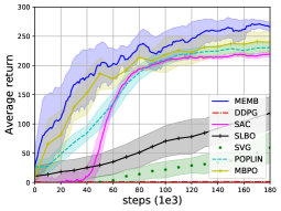
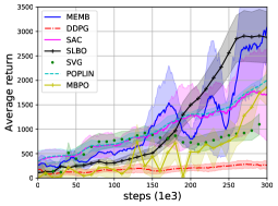
Comparison to state-of-the-art: We compare our algorithm with state-of-the-art model-free and model-based reinforcement learning algorithms in terms of sample complexity and performance. DDPG (Lillicrap etย al., 2015) and SAC (Haarnoja etย al., 2018) are two model-free reinforcement learning algorithms on continuous action tasks. SAC has shown its reliable performance and robustness on several benchmark tasks. Our algorithm also builds on the maximum entropy reinforcement learning framework and benefits from incorporating the model in the policy update. Four model-based reinforcement learning baselines are SVG (Heess etย al., 2015),SLBO (Luo etย al., 2018), MBPO (Janner etย al., 2019) and POPLIN (Wang and Ba, 2019). Notice in SVG, the algorithm just computes the gradient in the real trajectory, while our MEMB updates policy using the imaginary data $m$ times generated from the model. At the same time, we avoid the importance sampling by using the data from the learned model. SLBO is a model-base algorithm with performance guarantees that applies TRPO (Schulman etย al., 2015) on the data set generated from the rollout of the model. MBPO has the similar spirit but with SAC as the learning algorithm on the imaginary data.

For fairness, we compare the baseline without the ensemble learning techniques (Chua etย al., 2018). These techniques are known to reduce the model bias. We do not use distributed RL either to accelerate the training. We believe that the above-mentioned skills are orthogonal to our work and could be integrated into the future work to further improve the performance. We just compare this pure version of MEMB with other baselines. We also notice that some recent works in MBRL modify the benchmarks to shorten the task horizons and simplify the model problem while some work assume the true terminal condition is known to the algorithm (Wang etย al., 2019). On the contrary, we test our algorithm in the full-length tasks and do not have assumptions on the terminal condition.

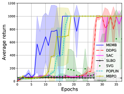
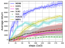
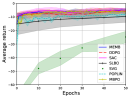
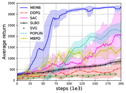
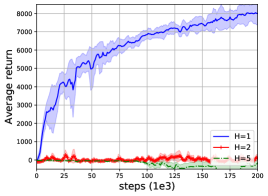
We present experimental results in Figure 1. In a simple task, InvertedPendulum, MEMB achieves the asymptotic result just using 16 epochs. In HalfCheetah, MEMBโ€™s performance is at around 8000 at 200k steps, while all the other baselinesโ€™ performance is below 5300. In Reacher, MEMB and SAC have similar performance. Both of them are better than other algorithms. In Hopper, the final performance of MEMB is around 3300. The runner-up is POPLIN whose final performance is around 2300. In Swimmer, the performance of MEMB is the best. In Walker2d, SLBO is slighter better than MEMB. Both of them achieve the average return of 2900 at 300k timesteps.

References

  • Asadi etย al. (2018) Kavosh Asadi, Dipendra Misra, and Michaelย L Littman. Lipschitz continuity in model-based reinforcement learning. ICML 2018, 2018.
  • Brockman etย al. (2016) Greg Brockman, Vicki Cheung, Ludwig Pettersson, Jonas Schneider, John Schulman, Jie Tang, and Wojciech Zaremba. Openai gym. arXiv preprint arXiv:1606.01540, 2016.
  • Chua etย al. (2018) Kurtland Chua, Roberto Calandra, Rowan McAllister, and Sergey Levine. Deep reinforcement learning in a handful of trials using probabilistic dynamics models. In Advances in Neural Information Processing Systems, pages 4754โ€“4765, 2018.
  • Clavera etย al. (2018) Ignasi Clavera, Jonas Rothfuss, John Schulman, Yasuhiro Fujita, Tamim Asfour, and Pieter Abbeel. Model-based reinforcement learning via meta-policy optimization. arXiv preprint arXiv:1809.05214, 2018.
  • Deisenroth and Rasmussen (2011) Marc Deisenroth and Carlย E Rasmussen. Pilco: A model-based and data-efficient approach to policy search. In Proceedings of the 28th International Conference on machine learning (ICML-11), pages 465โ€“472, 2011.
  • Feinberg etย al. (2018) Vย Feinberg, Aย Wan, Iย Stoica, MIย Jordan, JEย Gonzalez, and Sย Levine. Model-based value expansion for efficient model-free reinforcement learning. In Proceedings of the 35th International Conference on Machine Learning (ICML 2018), 2018.
  • Finn etย al. (2016) Chelsea Finn, Sergey Levine, and Pieter Abbeel. Guided cost learning: Deep inverse optimal control via policy optimization. In International Conference on Machine Learning, pages 49โ€“58, 2016.
  • Fox etย al. (2016) Roy Fox, Ari Pakman, and Naftali Tishby. Taming the noise in reinforcement learning via soft updates. UAI, 2016.
  • Fujimoto etย al. (2018) Scott Fujimoto, Herke van Hoof, and David Meger. Addressing function approximation error in actor-critic methods. arXiv preprint arXiv:1802.09477, 2018.
  • Gulrajani etย al. (2017) Ishaan Gulrajani, Faruk Ahmed, Martin Arjovsky, Vincent Dumoulin, and Aaronย C Courville. Improved training of wasserstein gans. In Advances in neural information processing systems, pages 5767โ€“5777, 2017.
  • Haarnoja etย al. (2017) Tuomas Haarnoja, Haoran Tang, Pieter Abbeel, and Sergey Levine. Reinforcement learning with deep energy-based policies. In Proceedings of the 34th International Conference on Machine Learning-Volume 70, pages 1352โ€“1361. JMLR. org, 2017.
  • Haarnoja etย al. (2018) Tuomas Haarnoja, Aurick Zhou, Pieter Abbeel, and Sergey Levine. Soft actor-critic: Off-policy maximum entropy deep reinforcement learning with a stochastic actor. arXiv preprint arXiv:1801.01290, 2018.
  • Heess etย al. (2015) Nicolas Heess, Gregory Wayne, David Silver, Timothy Lillicrap, Tom Erez, and Yuval Tassa. Learning continuous control policies by stochastic value gradients. In Advances in Neural Information Processing Systems, pages 2944โ€“2952, 2015.
  • Janner etย al. (2019) Michael Janner, Justin Fu, Marvin Zhang, and Sergey Levine. When to trust your model: Model-based policy optimization. In Advances in Neural Information Processing Systems, pages 12498โ€“12509, 2019.
  • Kalweit and Boedecker (2017) Gabriel Kalweit and Joschka Boedecker. Uncertainty-driven imagination for continuous deep reinforcement learning. In Conference on Robot Learning, pages 195โ€“206, 2017.
  • Kurutach etย al. (2018) Thanard Kurutach, Ignasi Clavera, Yan Duan, Aviv Tamar, and Pieter Abbeel. Model-ensemble trust-region policy optimization. arXiv preprint arXiv:1802.10592, 2018.
  • Levine (2018) Sergey Levine. Reinforcement learning and control as probabilistic inference: Tutorial and review. arXiv preprint arXiv:1805.00909, 2018.
  • Levine and Abbeel (2014) Sergey Levine and Pieter Abbeel. Learning neural network policies with guided policy search under unknown dynamics. In Advances in Neural Information Processing Systems, pages 1071โ€“1079, 2014.
  • Levine and Koltun (2013) Sergey Levine and Vladlen Koltun. Guided policy search. In International Conference on Machine Learning, pages 1โ€“9, 2013.
  • Lillicrap etย al. (2015) Timothyย P Lillicrap, Jonathanย J Hunt, Alexander Pritzel, Nicolas Heess, Tom Erez, Yuval Tassa, David Silver, and Daan Wierstra. Continuous control with deep reinforcement learning. arXiv preprint arXiv:1509.02971, 2015.
  • Luo etย al. (2018) Yuping Luo, Huazhe Xu, Yuanzhi Li, Yuandong Tian, Trevor Darrell, and Tengyu Ma. Algorithmic framework for model-based deep reinforcement learning with theoretical guarantees. arXiv preprint arXiv:1807.03858, 2018.
  • Mnih etย al. (2015) Volodymyr Mnih, Koray Kavukcuoglu, David Silver, Andreiย A Rusu, Joel Veness, Marcย G Bellemare, Alex Graves, Martin Riedmiller, Andreasย K Fidjeland, Georg Ostrovski, etย al. Human-level control through deep reinforcement learning. Nature, 518(7540):529, 2015.
  • Nagabandi etย al. (2018) Anusha Nagabandi, Gregory Kahn, Ronaldย S Fearing, and Sergey Levine. Neural network dynamics for model-based deep reinforcement learning with model-free fine-tuning. In 2018 IEEE International Conference on Robotics and Automation (ICRA), pages 7559โ€“7566. IEEE, 2018.
  • Richards (2005) Arthurย George Richards. Robust constrained model predictive control. PhD thesis, Massachusetts Institute of Technology, 2005.
  • Schulman etย al. (2015) John Schulman, Sergey Levine, Pieter Abbeel, Michael Jordan, and Philipp Moritz. Trust region policy optimization. In International conference on machine learning, pages 1889โ€“1897, 2015.
  • Sutton (1990) Richardย S Sutton. Integrated architectures for learning, planning, and reacting based on approximating dynamic programming. In Machine Learning Proceedings 1990, pages 216โ€“224. Elsevier, 1990.
  • Tassa etย al. (2012) Yuval Tassa, Tom Erez, and Emanuel Todorov. Synthesis and stabilization of complex behaviors through online trajectory optimization. In 2012 IEEE/RSJ International Conference on Intelligent Robots and Systems, pages 4906โ€“4913. IEEE, 2012.
  • Todorov etย al. (2012) Emanuel Todorov, Tom Erez, and Yuval Tassa. Mujoco: A physics engine for model-based control. In 2012 IEEE/RSJ International Conference on Intelligent Robots and Systems, pages 5026โ€“5033. IEEE, 2012.
  • Villani (2010) Cรฉdric Villani. Optimal transport: old and new. Bull. Amer. Math. Soc, 47:723โ€“727, 2010.
  • Wang and Ba (2019) Tingwu Wang and Jimmy Ba. Exploring model-based planning with policy networks. ICLR 2020, 2019.
  • Wang etย al. (2019) Tingwu Wang, Xuchan Bao, Ignasi Clavera, Jerrick Hoang, Yeming Wen, Eric Langlois, Shunshi Zhang, Guodong Zhang, Pieter Abbeel, and Jimmy Ba. Benchmarking model-based reinforcement learning. arXiv preprint arXiv:1907.02057, 2019.
  • Ziebart etย al. (2008) Brianย D Ziebart, Andrew Maas, Jย Andrew Bagnell, and Anindย K Dey. Maximum entropy inverse reinforcement learning. 2008.

Appendix A Related work

There are a plethora of works on MBRL. They can be classified into several categories depending on the way to utilize the model, to search the optimal policy or the function approximator of the dynamics model. Iterative Linear Quadratic-Gaussian (iLQG) (Tassa etย al., 2012) assumes that the true dynamics are known to the agent. It approximates the dynamics with linear functions and the reward function with quadratic functions. Hence the problem can be transferred into the classic LQR problem. In Guided Policy Search (Levine and Koltun, 2013; Levine and Abbeel, 2014; Finn etย al., 2016), the system dynamics are modeled with the time-varying Gaussian-linear model. It approximated the policy with a neural network $\pi$ by minimizing the KL divergence between iLQG and $\pi$. A regularization term is augmented into the reward function to avoid the over-confidence on the policy optimization. Nonlinear function approximators can be leveraged to model more complicated dynamics. Deisenroth and Rasmussen (2011) use Gaussian processes to model the dynamics of the environment. The policy gradient can be computed analytically along the training trajectory. However, it may suffer from the curse of dimensionality which hinders its applicability in the real problem. Recently, more and more works incorporate the deep neural network into MBRL. Heess etย al. (2015) model the dynamics and reward with neural networks, and compute the gradient with the true data. Richards (2005); Nagabandi etย al. (2018) optimize the action sequence to maximize the expected planning reward along with the learned dynamics model and then the policy is fine-tuned with TRPO. Luo etย al. (2018); Chua etย al. (2018); Kurutach etย al. (2018); Janner etย al. (2019) use the current policy to gather the data from the interaction with the environment and then learn the dynamics model. In the next step, the policy is improved (trained by the model-free reinforcement learning algorithm) with a large amount of imaginary data generated by the learned model. MEMB may reduce to their work by updating the policy with a model-free algorithm. Janner etย al. (2019) provide an error bound on the long term return of the k-step rollout given that the total variation of model bias and policy distribution are bounded by $\epsilon$. However, as we discussed, total variation may not be a good measure to describe the difference of learned model and true model especially when the support of the distributions is disjoint. Ensemble learning can also be applied to further reduce the model error. Asadi etย al. (2018) leverage the Lipschitz model to analyze the model bias in the long term return. Our work consider the both model bias and the distribution shift on the policy. In addition, we analyze the k-step rollout while Asadi etย al. (2018) just gives the result on full rollout.

Appendix B Ablation Study

B.1 How to utilize the imaginary data

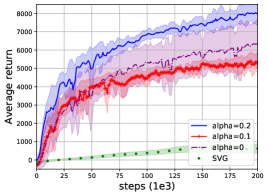
In this section, we make the ablation study to understand how much imaginary data we should include in the algorithm. Remind that in our algorithm, the model is embedded in the Soft Bellman equation in the policy update step, which means we fully trust the model to compute the policy gradient. This way to utilize the imaginary data would improve the sample-efficiency. To confirm our claim, we compare the MEMB with SVG on the task HalfCheetah. Notice when we just utilize the real trajectory in the policy update, MEMB reduces to the SVG444It still has some difference such as the update rule of Q and V function. To remove the effect of the entropy regularization, we vary $\alpha$ (the regularizer parameter of entropy) in MEMB. When $\alpha=0$, it reduces to the non-regularized formulation. In that case, we add the noise in policy for the exploration. We report the result in panel (a) of Fig 2. It is clear that using imaginary data in policy update improves the learning with a wide margin.
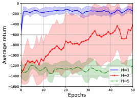
In Section 3.2, we train $Q$ and $V$ with the true data set. In the experiment, we also try the value expansion introduced in (Feinberg etย al., 2018). We test the algorithm with value expansion, particularly with horizon $H=2$ and $H=5$. Our conclusion is that including the imaginary data to train the value function in our algorithm would hurt the performance, especially in the complex tasks. We demonstrate the performance of MEMB with value expansion in panel (b) and (c) of Figure 2. We first test the algorithm on a simple task Pendulum from OpenAI gym (Brockman etย al., 2016) and show the result in Panel (b) of Figure 2. MEMB with $H=1$ converges to the optimal policy within several epochs. When we increase the value of $H$, the performance decreases. Then we evaluate the performance of value expansion in a complex task HalfCheetah from the Mujoco environment (Todorov etย al., 2012) in panel (c) of Figure 2. In this task, value expansion with $H=2$ and $H=5$ does not work at all. The reason would be that the dynamics model of HalfCheetah introduces more significant model bias comparing to the simple task Pendulum. Thus training both policy and value function in the imaginary data set may cause a large error in policy gradient.

Refer to caption
(a) HalfCheetah (policy)
Refer to caption
(b) Pendulum (value)
Refer to caption
(c) HalfCheetah (value)
Figure 2: Ablation study. In (a) we do the ablation study on the effect of the imaginary data on policy learning. In (b) and (c) we do ablation study on the value function learning with different length of rollout H. The x-axis is the training step and the y-axis is the reward.

B.2 Model Error

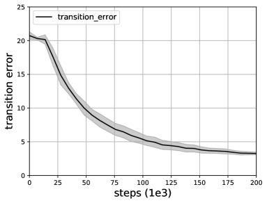
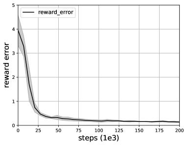
We test the difference between the true model and learned model (using Wasserstein distance), i.e., model error. In particular, we record the learned model by MEMB every 10 epochs and then randomly sample the state action pair (s,a)๐‘ ๐‘Ž(s,a). Feed this pair to the learn model we can obtain the predicted next state s^โ€ฒsuperscript^๐‘ โ€ฒ\hat{s}^{\prime}, which is used to compared with the true next state sโ€ฒsuperscript๐‘ โ€ฒs^{\prime}. The error is averaged over state action pair. We do similar things on the reward model. Result are tested on five trials using five different random seeds. They are reported in Figure 3.

Refer to caption
(a) Transition model error
Refer to caption
(b) Reward model error
Figure 3: Model error. We calculate the model error on the environment of HalfCheetah.

B.3 Plug The True Model Into MEMB

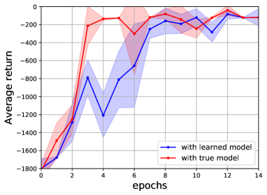
It is interesting to see the performance of MEMB if we plugin the true model in the algorithm. Since the dynamic in Mujoco is complicated, we just test a simple task pendulum. Intuitively, MEMB with true model should have better performance than the MEMB with learned one. We verify this in the Figure 4.

Refer to caption
Figure 4: MEMB with the true model vs MEMB with the learned model in pendulum

B.4 Asymptotic Performance

We evaluate the asymptotic behavior of model-free RL (particularly SAC) and MEMB agents through 2000 epoch of training (20M steps) on four simulation environments to see the asymptotic result. The SAC agent achieves $9453.32\pm 219.34$ in HalfCheetah, $4182.07\pm 63.23$ in Walker2d, $3433.03\pm 18.05$ in Hopper, $310.3\pm 4.60$ in Swimmer. The MEMB agent achieves $8813.14\pm 53.04$ in HalfCheetah, $3544.3\pm 252.3$ in Walker2d, $3265\pm 12.65$ in Hopper, $307.57\pm 8.97$ in Swimmer. In general, there is a small gap between the asymptotic performance between MBRL and MFRL. It is well expected since the learned model is not accurate.

Appendix C Environment Overview and Hyperparameter Setting

In this section, we provide an overview of simulation environment in Table 1. The hyperparameter setting for each environment is shown in Table 2.

Environment Name Observation Space Dimension Action Space Dimension Horizon
Pendulum 3 1 200
InvertedPendulum 4 1 1000
HalfCheetah 17 6 1000
Hopper 11 3 1000
Walker2D 17 6 1000
Swimmer 8 2 1000
Reacher 11 2 50
Table 1: The observation space dimension, action space dimension, and horizon for each simulation environment implemented in the experiment and ablation study.
Pendulum InvertedPendulum HalfCheetah Hopper Walker2D Swimmer Reacher
Epoch 50 40 200 300 180 50
Policy Learning Rate
0.0003
Value Learning Rate
0.0003 0.001 0.001 0.0003 0.0003 0.0003
Model
Learning Rate
0.0003 0.0001 0.0001 0.0001
Alpha value
(in entropy term)
0.2 0.1 0.4 0.2 0.2
environment steps
per epoch
1000 50
Value and Policy
Network Architecture
(256,256)
Model
Network Architecture
(32,16) (256,128) (256,256) (256,128)
Train Actor-critic
Times ($m$)
5 1 5 3 5 5
Table 2: The hyper-parameter used in training MEMB algorithm for each simulation environment. The number in policy, value, and model network architecture indicate the size of hidden units in each layer of MLP. The ReLu activation function is implemented in all architecture.

Appendix D Proof

In this section, we give the proof of the theorem in the main paper. To start with, we give the definition of the Wasserstein distance and its dual form, since we will use it frequently in the following discussion.

Definition: Give a meritc space $(M,d)$ and the set $\mathbb{P}(M)$ of probability measures on $M$, the Wasserstein metric between two probability distributions $\mu_{1}$ and $\mu_{2}$ in $\mathbb{P}(M)$ is defined as

$$W(\mu_{1},\mu_{2}):=\inf_{j\in\Sigma}\int\int p(x,y)d(x,y)dxdy,$$ (10)

where $\Sigma$ denotes the collection of all joint distributions $p$ with marginal $\mu_{1}$ and $\mu_{2}$.

The dual presentation is a special case of the duality theorem of Kantorovich and Rubinstein Villani (2010).

Wโ€‹(ฮผ1,ฮผ2)=supโ€–fโ€–โ‰ค1โˆซfโ€‹(s)โ€‹(ฮผ1โ€‹(s)โˆ’ฮผ2โ€‹(s))โ€‹๐‘‘s๐‘Šsubscript๐œ‡1subscript๐œ‡2subscriptsupremumnorm๐‘“1๐‘“๐‘ subscript๐œ‡1๐‘ subscript๐œ‡2๐‘ differential-d๐‘ W(\mu_{1},\mu_{2})=\sup_{\|f\|\leq 1}\int f(s)(\mu_{1}(s)-\mu_{2}(s))ds (11)

where $\|f\|\leq 1$ means the function $f$ is $1$-Lipschitz.

The first lemma is well known. It says the Lipschitz constant of a composition function is the product of Lipschitz constants of two functions.

Lemma 1.

Define three metric spaces $(M_{1},d_{1}),(M_{2},d_{2}),(M_{3},d_{3})$. Define Lipschitz function $f:M_{2}\rightarrow M_{3}$ and $g:M_{1}\rightarrow M_{2}$ with constant $K_{f}$, $K_{g}$. Then $h:f\circ g$ is Lipschitz with constant $K_{h}\leq K_{f}K_{g}$

Proof.
$$\begin{split}K_{h}=&\sup_{x_{1},x_{2}}d_{3}\big{(}f(g(x_{1}),f(g(x_{2})))\big{)}/d(x_{1},x_{2})\\ =&\sup_{x_{1},x_{2}}\frac{d_{2}(g(x_{1}),g(x_{2}))}{d_{1}(x_{1},x_{2})}\frac{d_{3}\big{(}f(g(x_{1}),f(g(x_{2}))\big{)}}{d_{2}(g(x_{1}),g(x_{2}))}\\ \leq&\sup_{x_{1},x_{2}}\frac{d_{2}(g(x_{1}),g(x_{2}))}{d_{1}(x_{1},x_{2})}\sup_{y_{1},y_{2}}\frac{d_{3}(y_{1},y_{2})}{d_{2}(y_{1},y_{2})}\leq K_{g}K_{f}\end{split}$$ (12)

โˆŽ

Lemma 2.

Suppose we have two joint distribution p1โ€‹(s,a)=p1โ€‹(s)โ€‹ฯ€1โ€‹(a|s)subscript๐‘1๐‘ ๐‘Žsubscript๐‘1๐‘ subscript๐œ‹1conditional๐‘Ž๐‘ p_{1}(s,a)=p_{1}(s)\pi_{1}(a|s), p2โ€‹(s,a)=p2โ€‹(s)โ€‹ฯ€2โ€‹(a|s)subscript๐‘2๐‘ ๐‘Žsubscript๐‘2๐‘ subscript๐œ‹2conditional๐‘Ž๐‘ p_{2}(s,a)=p_{2}(s)\pi_{2}(a|s). We further assume that Wโ€‹(pโ€‹(s1),pโ€‹(s2))โ‰คฯตm๐‘Š๐‘subscript๐‘ 1๐‘subscript๐‘ 2subscriptitalic-ฯต๐‘šW(p(s_{1}),p(s_{2}))\leq\epsilon_{m} and Wโ€‹(ฯ€1โ€‹(a|s),ฯ€2โ€‹(a|s))โ‰คฯตฯ€๐‘Šsubscript๐œ‹1conditional๐‘Ž๐‘ subscript๐œ‹2conditional๐‘Ž๐‘ subscriptitalic-ฯต๐œ‹W(\pi_{1}(a|s),\pi_{2}(a|s))\leq\epsilon_{\pi}. Then we have Wโ€‹(p1โ€‹(s,a),p2โ€‹(s,a))โ‰คฯตฯ€+Kฯ€โ€‹ฯตm๐‘Šsubscript๐‘1๐‘ ๐‘Žsubscript๐‘2๐‘ ๐‘Žsubscriptitalic-ฯต๐œ‹subscript๐พ๐œ‹subscriptitalic-ฯต๐‘šW(p_{1}(s,a),p_{2}(s,a))\leq\epsilon_{\pi}+K_{\pi}\epsilon_{m}.

Proof.

Using the triangle inequality, we have

Wโ€‹(p1โ€‹(s,a),p2โ€‹(s,a))โ‰คWโ€‹(pโ€‹(s1)โ€‹ฯ€1โ€‹(a|s),p1โ€‹(s)โ€‹ฯ€2โ€‹(a|s))+Wโ€‹(p1โ€‹(s)โ€‹ฯ€2โ€‹(a|s),p2โ€‹(s)โ€‹ฯ€2โ€‹(a|s)).๐‘Šsubscript๐‘1๐‘ ๐‘Žsubscript๐‘2๐‘ ๐‘Ž๐‘Š๐‘subscript๐‘ 1subscript๐œ‹1conditional๐‘Ž๐‘ subscript๐‘1๐‘ subscript๐œ‹2conditional๐‘Ž๐‘ ๐‘Šsubscript๐‘1๐‘ subscript๐œ‹2conditional๐‘Ž๐‘ subscript๐‘2๐‘ subscript๐œ‹2conditional๐‘Ž๐‘ W(p_{1}(s,a),p_{2}(s,a))\leq W(p(s_{1})\pi_{1}(a|s),p_{1}(s)\pi_{2}(a|s))+W(p_{1}(s)\pi_{2}(a|s),p_{2}(s)\pi_{2}(a|s)).

Now we bound the first term and second term respectively. For the first term, according to the dual form of the Wasserstein distance, we have

Wโ€‹(p1โ€‹(s)โ€‹ฯ€1โ€‹(a|s),p1โ€‹(s)โ€‹ฯ€2โ€‹(a|s))=supโ€–fโ€–โ‰ค1โˆซโˆซfโ€‹(s,a)โ€‹p1โ€‹(s)โ€‹(ฯ€1โ€‹(a|s)โˆ’ฯ€2โ€‹(a|s))โ€‹๐‘‘aโ€‹๐‘‘s.๐‘Šsubscript๐‘1๐‘ subscript๐œ‹1conditional๐‘Ž๐‘ subscript๐‘1๐‘ subscript๐œ‹2conditional๐‘Ž๐‘ subscriptsupremumnorm๐‘“1๐‘“๐‘ ๐‘Žsubscript๐‘1๐‘ subscript๐œ‹1conditional๐‘Ž๐‘ subscript๐œ‹2conditional๐‘Ž๐‘ differential-d๐‘Ždifferential-d๐‘ \begin{split}&W(p_{1}(s)\pi_{1}(a|s),p_{1}(s)\pi_{2}(a|s))=\sup_{\|f\|\leq 1}\int\int f(s,a)p_{1}(s)(\pi_{1}(a|s)-\pi_{2}(a|s))dads\\ .\end{split} (13)

Notice it is easy to verify that if fโ€‹(s,a)๐‘“๐‘ ๐‘Žf(s,a) is a 1-Lipschitz function w.r.t. (s,a)๐‘ ๐‘Ž(s,a), then for a fixed $a$, fโ€‹(s,a)๐‘“๐‘ ๐‘Žf(s,a) (we denote it as fsโ€‹(a)subscript๐‘“๐‘ ๐‘Žf_{s}(a)) is also a 1-Lipschitz function w.r.t $a$. Thus $\forall f\in\{f:\|f\|\leq 1\}$, we have

โˆซโˆซfโ€‹(s,a)โ€‹p1โ€‹(s)โ€‹(ฯ€1โ€‹(a|s)โˆ’ฯ€2โ€‹(a|s))โ€‹๐‘‘aโ€‹๐‘‘s=โˆซp1โ€‹(s)โ€‹โˆซfsโ€‹(a)โ€‹(ฯ€1โ€‹(a|s)โˆ’ฯ€2โ€‹(a|s))โ€‹๐‘‘aโ€‹๐‘‘sโ‰คโˆซp1โ€‹(s)โ€‹Wโ€‹(ฯ€1โ€‹(a|s),ฯ€2โ€‹(a|s))โ€‹๐‘‘s=ฯตฯ€.๐‘“๐‘ ๐‘Žsubscript๐‘1๐‘ subscript๐œ‹1conditional๐‘Ž๐‘ subscript๐œ‹2conditional๐‘Ž๐‘ differential-d๐‘Ždifferential-d๐‘ subscript๐‘1๐‘ subscript๐‘“๐‘ ๐‘Žsubscript๐œ‹1conditional๐‘Ž๐‘ subscript๐œ‹2conditional๐‘Ž๐‘ differential-d๐‘Ždifferential-d๐‘ subscript๐‘1๐‘ ๐‘Šsubscript๐œ‹1conditional๐‘Ž๐‘ subscript๐œ‹2conditional๐‘Ž๐‘ differential-d๐‘ subscriptitalic-ฯต๐œ‹\begin{split}&\int\int f(s,a)p_{1}(s)(\pi_{1}(a|s)-\pi_{2}(a|s))dads\\ =&\int p_{1}(s)\int f_{s}(a)(\pi_{1}(a|s)-\pi_{2}(a|s))dads\\ \leq&\int p_{1}(s)W(\pi_{1}(a|s),\pi_{2}(a|s))ds=\epsilon_{\pi}.\end{split} (14)

We then bound the second term in the following way.

Wโ€‹(p1โ€‹(s)โ€‹ฯ€2โ€‹(a|s),p2โ€‹(s)โ€‹ฯ€2โ€‹(a|s))=supโ€–fโ€–โ‰ค1โˆซโˆซfโ€‹(s,a)โ€‹(p1โ€‹(s)โˆ’p2โ€‹(s))โ€‹ฯ€2โ€‹(a|s)โ€‹๐‘‘aโ€‹๐‘‘s=(1)supโ€–fโ€–โ‰ค1โˆซโˆซfโ€‹(s,a)โ€‹โˆ‘gฯ€โ€‹(fฯ€)โ€‹๐Ÿ™โ€‹(fฯ€โ€‹(s)=a)โ€‹(p1โ€‹(s)โˆ’p2โ€‹(s))โ€‹dโ€‹sโ€‹dโ€‹a=supโ€–fโ€–โ‰ค1โˆซโˆ‘fฯ€gฯ€โ€‹(fฯ€)โ€‹fโ€‹(s,fฯ€โ€‹(s))โ€‹(p1โ€‹(s)โˆ’p2โ€‹(s))โ€‹dโ€‹sโ‰คโˆ‘fฯ€gฯ€โ€‹(fฯ€)โ€‹supโ€–fโ€–โ‰ค1โˆซfโ€‹(s,fฯ€โ€‹(s))โ€‹(p1โ€‹(s)โˆ’p2โ€‹(s))โ€‹๐‘‘s=โˆ‘fฯ€gฯ€โ€‹(fฯ€)โ€‹Kฯ€โ€‹supโ€–fโ€–โ‰ค1โˆซfโ€‹(s,fฯ€โ€‹(s))Kฯ€โ€‹(p1โ€‹(s)โˆ’p2โ€‹(s))โ€‹๐‘‘s=(2)โˆ‘fฯ€gฯ€โ€‹(fฯ€)โ€‹Kฯ€โ€‹Wโ€‹(p1โ€‹(s),p2โ€‹(s))โ‰คKฯ€โ€‹ฯตm๐‘Šsubscript๐‘1๐‘ subscript๐œ‹2conditional๐‘Ž๐‘ subscript๐‘2๐‘ subscript๐œ‹2conditional๐‘Ž๐‘ subscriptsupremumnorm๐‘“1๐‘“๐‘ ๐‘Žsubscript๐‘1๐‘ subscript๐‘2๐‘ subscript๐œ‹2conditional๐‘Ž๐‘ differential-d๐‘Ždifferential-d๐‘ 1subscriptsupremumnorm๐‘“1๐‘“๐‘ ๐‘Žsubscript๐‘”๐œ‹subscript๐‘“๐œ‹1subscript๐‘“๐œ‹๐‘ ๐‘Žsubscript๐‘1๐‘ subscript๐‘2๐‘ ๐‘‘๐‘ ๐‘‘๐‘Žsubscriptsupremumnorm๐‘“1subscriptsubscript๐‘“๐œ‹subscript๐‘”๐œ‹subscript๐‘“๐œ‹๐‘“๐‘ subscript๐‘“๐œ‹๐‘ subscript๐‘1๐‘ subscript๐‘2๐‘ ๐‘‘๐‘ subscriptsubscript๐‘“๐œ‹subscript๐‘”๐œ‹subscript๐‘“๐œ‹subscriptsupremumnorm๐‘“1๐‘“๐‘ subscript๐‘“๐œ‹๐‘ subscript๐‘1๐‘ subscript๐‘2๐‘ differential-d๐‘ subscriptsubscript๐‘“๐œ‹subscript๐‘”๐œ‹subscript๐‘“๐œ‹subscript๐พ๐œ‹subscriptsupremumnorm๐‘“1๐‘“๐‘ subscript๐‘“๐œ‹๐‘ subscript๐พ๐œ‹subscript๐‘1๐‘ subscript๐‘2๐‘ differential-d๐‘ 2subscriptsubscript๐‘“๐œ‹subscript๐‘”๐œ‹subscript๐‘“๐œ‹subscript๐พ๐œ‹๐‘Šsubscript๐‘1๐‘ subscript๐‘2๐‘ subscript๐พ๐œ‹subscriptitalic-ฯต๐‘š\begin{split}W(p_{1}(s)\pi_{2}(a|s),p_{2}(s)\pi_{2}(a|s))=&\sup_{\|f\|\leq 1}\int\int f(s,a)(p_{1}(s)-p_{2}(s))\pi_{2}(a|s)dads\\ \overset{(1)}{=}&\sup_{\|f\|\leq 1}\int\int f(s,a)\sum g_{\pi}(f_{\pi})\mathbbm{1}(f_{\pi}(s)=a)\big{(}p_{1}(s)-p_{2}(s)\big{)}dsda\\ =&\sup_{\|f\|\leq 1}\int\sum_{f_{\pi}}g_{\pi}(f_{\pi})f(s,f_{\pi}(s))(p_{1}(s)-p_{2}(s))ds\\ \leq&\sum_{f_{\pi}}g_{\pi}(f_{\pi})\sup_{\|f\|\leq 1}\int f(s,f_{\pi}(s))(p_{1}(s)-p_{2}(s))ds\\ =&\sum_{f_{\pi}}g_{\pi}(f_{\pi})K_{\pi}\sup_{\|f\|\leq 1}\int\frac{f(s,f_{\pi}(s))}{K_{\pi}}(p_{1}(s)-p_{2}(s))ds\\ \overset{(2)}{=}&\sum_{f_{\pi}}g_{\pi}(f_{\pi})K_{\pi}W(p_{1}(s),p_{2}(s))\\ \leq&K_{\pi}\epsilon_{m}\end{split} (15)

where (1) holds using the assumption $\pi$ is in the Lipschitz class. (2) uses the fact that fโ€‹(s,fฯ€โ€‹(s))Kฯ€๐‘“๐‘ subscript๐‘“๐œ‹๐‘ subscript๐พ๐œ‹\frac{f(s,f_{\pi}(s))}{K_{\pi}} is 1 Lipschitz, which holds using the similar argument in Lemma 1.

Combine two pieces together, we obtain the result. โˆŽ

Lemma 3.

Define p1,ฯ€1โ€‹(sโ€ฒ|s)=โˆซp1โ€‹(sโ€ฒ|s,a)โ€‹ฯ€1โ€‹(a|s)โ€‹๐‘‘asubscript๐‘1subscript๐œ‹1conditionalsuperscript๐‘ โ€ฒ๐‘ subscript๐‘1conditionalsuperscript๐‘ โ€ฒ๐‘ ๐‘Žsubscript๐œ‹1conditional๐‘Ž๐‘ differential-d๐‘Žp_{1,\pi_{1}}(s^{\prime}|s)=\int p_{1}(s^{\prime}|s,a)\pi_{1}(a|s)da and p2,ฯ€2โ€‹(sโ€ฒ|s)=โˆซp2โ€‹(sโ€ฒ|s,a)โ€‹ฯ€2โ€‹(a|s)โ€‹๐‘‘asubscript๐‘2subscript๐œ‹2conditionalsuperscript๐‘ โ€ฒ๐‘ subscript๐‘2conditionalsuperscript๐‘ โ€ฒ๐‘ ๐‘Žsubscript๐œ‹2conditional๐‘Ž๐‘ differential-d๐‘Žp_{2,\pi_{2}}(s^{\prime}|s)=\int p_{2}(s^{\prime}|s,a)\pi_{2}(a|s)da. Suppose Wโ€‹(p1โ€‹(sโ€ฒ|s,a),p2โ€‹(sโ€ฒ|s,a))โ‰คฯตm๐‘Šsubscript๐‘1conditionalsuperscript๐‘ โ€ฒ๐‘ ๐‘Žsubscript๐‘2conditionalsuperscript๐‘ โ€ฒ๐‘ ๐‘Žsubscriptitalic-ฯต๐‘šW(p_{1}(s^{\prime}|s,a),p_{2}(s^{\prime}|s,a))\leq\epsilon_{m}, Wโ€‹(ฯ€1โ€‹(a|s),Wโ€‹(ฯ€2โ€‹(a|s)))โ‰คฯตฯ€๐‘Šsubscript๐œ‹1conditional๐‘Ž๐‘ ๐‘Šsubscript๐œ‹2conditional๐‘Ž๐‘ subscriptitalic-ฯต๐œ‹W(\pi_{1}(a|s),W(\pi_{2}(a|s)))\leq\epsilon_{\pi}, then we have

Wโ€‹(p1,ฯ€1โ€‹(sโ€ฒ|s),p2,ฯ€2โ€‹(sโ€ฒ|s))โ‰คKmโ€‹ฯตฯ€+ฯตm๐‘Šsubscript๐‘1subscript๐œ‹1conditionalsuperscript๐‘ โ€ฒ๐‘ subscript๐‘2subscript๐œ‹2conditionalsuperscript๐‘ โ€ฒ๐‘ subscript๐พ๐‘šsubscriptitalic-ฯต๐œ‹subscriptitalic-ฯต๐‘šW(p_{1,\pi_{1}}(s^{\prime}|s),p_{2,\pi_{2}}(s^{\prime}|s))\leq K_{m}\epsilon_{\pi}+\epsilon_{m}

.

Proof.

We define a reference probability distribution p1,ฯ€2โ€‹(sโ€ฒ|s)=โˆซp1โ€‹(sโ€ฒ|s,a)โ€‹ฯ€2โ€‹(a|s)โ€‹๐‘‘asubscript๐‘1subscript๐œ‹2conditionalsuperscript๐‘ โ€ฒ๐‘ subscript๐‘1conditionalsuperscript๐‘ โ€ฒ๐‘ ๐‘Žsubscript๐œ‹2conditional๐‘Ž๐‘ differential-d๐‘Žp_{1,\pi_{2}}(s^{\prime}|s)=\int p_{1}(s^{\prime}|s,a)\pi_{2}(a|s)da. Using the triangle inequaity, we have

$$W(p_{1,\pi_{1}}(s^{\prime}|s)),p_{2,\pi_{2}}(s^{\prime}|s))\leq W(p_{1,\pi_{1}}(s^{\prime}|s),p_{1,\pi_{2}}(s^{\prime}|s))+W(p_{1,\pi_{2}}(s^{\prime}|s),p_{2,\pi_{2}}(s^{\prime}|s)).$$

Thus we just need to bound the two terms on the right hand side.

For the first term, according to the definition of the Wasserstein distance, we have

Wโ€‹(p1,ฯ€1โ€‹(sโ€ฒ|s),p1,ฯ€2โ€‹(sโ€ฒ|s))โ‰คsupโ€–bโ€–โ‰ค1โˆซ(โˆซp1โ€‹(sโ€ฒ|s,a)โ€‹ฯ€1โ€‹(a|s)โˆ’p1โ€‹(sโ€ฒ|s,a)โ€‹ฯ€2โ€‹(a|s)โ€‹dโ€‹a)โ€‹bโ€‹(sโ€ฒ)โ€‹๐‘‘sโ€ฒโ€‹๐‘‘a=(1)supโ€–bโ€–โ‰ค1โˆซโˆซโˆ‘fmgmโ€‹(fm)โ€‹(ฯ€1โ€‹(a|s)โˆ’ฯ€2โ€‹(a|s))โ€‹๐Ÿ™โ€‹(fmโ€‹(a,s)=sโ€ฒ)โ€‹bโ€‹(sโ€ฒ)โ€‹dโ€‹sโ€ฒโ€‹dโ€‹a=supโ€–bโ€–โ‰ค1โˆ‘fmgmโ€‹(fm)โ€‹โˆซ(ฯ€1โ€‹(a|s)โˆ’ฯ€2โ€‹(a|s))โ€‹bโ€‹(fmโ€‹(s,a))โ€‹๐‘‘aโ‰คโˆ‘fmgmโ€‹(fm)โ€‹Kmโ€‹supโ€–bโ€–โ‰ค1โˆซ(ฯ€1โ€‹(a|s)โˆ’ฯ€2โ€‹(a|s))โ€‹bโ€‹(fmโ€‹(a,s))Kmโ€‹๐‘‘aโ‰ค(2)โˆ‘fmgmโ€‹(fm)โ€‹Kmโ€‹Wโ€‹(ฯ€1โ€‹(a|s),ฯ€2โ€‹(a|s))โ‰คKmโ€‹ฯตฯ€.๐‘Šsubscript๐‘1subscript๐œ‹1conditionalsuperscript๐‘ โ€ฒ๐‘ subscript๐‘1subscript๐œ‹2conditionalsuperscript๐‘ โ€ฒ๐‘ subscriptsupremumnorm๐‘1subscript๐‘1conditionalsuperscript๐‘ โ€ฒ๐‘ ๐‘Žsubscript๐œ‹1conditional๐‘Ž๐‘ subscript๐‘1conditionalsuperscript๐‘ โ€ฒ๐‘ ๐‘Žsubscript๐œ‹2conditional๐‘Ž๐‘ ๐‘‘๐‘Ž๐‘superscript๐‘ โ€ฒdifferential-dsuperscript๐‘ โ€ฒdifferential-d๐‘Ž1subscriptsupremumnorm๐‘1subscriptsubscript๐‘“๐‘šsubscript๐‘”๐‘šsubscript๐‘“๐‘šsubscript๐œ‹1conditional๐‘Ž๐‘ subscript๐œ‹2conditional๐‘Ž๐‘ 1subscript๐‘“๐‘š๐‘Ž๐‘ superscript๐‘ โ€ฒ๐‘superscript๐‘ โ€ฒ๐‘‘superscript๐‘ โ€ฒ๐‘‘๐‘Žsubscriptsupremumnorm๐‘1subscriptsubscript๐‘“๐‘šsubscript๐‘”๐‘šsubscript๐‘“๐‘šsubscript๐œ‹1conditional๐‘Ž๐‘ subscript๐œ‹2conditional๐‘Ž๐‘ ๐‘subscript๐‘“๐‘š๐‘ ๐‘Ždifferential-d๐‘Žsubscriptsubscript๐‘“๐‘šsubscript๐‘”๐‘šsubscript๐‘“๐‘šsubscript๐พ๐‘šsubscriptsupremumnorm๐‘1subscript๐œ‹1conditional๐‘Ž๐‘ subscript๐œ‹2conditional๐‘Ž๐‘ ๐‘subscript๐‘“๐‘š๐‘Ž๐‘ subscript๐พ๐‘šdifferential-d๐‘Ž2subscriptsubscript๐‘“๐‘šsubscript๐‘”๐‘šsubscript๐‘“๐‘šsubscript๐พ๐‘š๐‘Šsubscript๐œ‹1conditional๐‘Ž๐‘ subscript๐œ‹2conditional๐‘Ž๐‘ subscript๐พ๐‘šsubscriptitalic-ฯต๐œ‹\begin{split}&W(p_{1,\pi_{1}}(s^{\prime}|s),p_{1,\pi_{2}}(s^{\prime}|s))\\ \leq&\sup_{\|b\|\leq 1}\int\big{(}\int p_{1}(s^{\prime}|s,a)\pi_{1}(a|s)-p_{1}(s^{\prime}|s,a)\pi_{2}(a|s)da\big{)}b(s^{\prime})ds^{\prime}da\\ \overset{(1)}{=}&\sup_{\|b\|\leq 1}\int\int\sum_{f_{m}}g_{m}(f_{m})(\pi_{1}(a|s)-\pi_{2}(a|s))\mathbbm{1}(f_{m}(a,s)=s^{\prime})b(s^{\prime})ds^{\prime}da\\ =&\sup_{\|b\|\leq 1}\sum_{f_{m}}g_{m}(f_{m})\int(\pi_{1}(a|s)-\pi_{2}(a|s))b(f_{m}(s,a))da\\ \leq&\sum_{f_{m}}g_{m}(f_{m})K_{m}\sup_{\|b\|\leq 1}\int(\pi_{1}(a|s)-\pi_{2}(a|s))\frac{b(f_{m}(a,s))}{K_{m}}da\\ \overset{(2)}{\leq}&\sum_{f_{m}}g_{m}(f_{m})K_{m}W(\pi_{1}(a|s),\pi_{2}(a|s))\\ \leq&K_{m}\epsilon_{\pi}.\end{split} (16)

where (1) holds using the assumption that the transition model is Lipschitz. (2) holds from the fact that bโ€‹(fmโ€‹(a,s))/Km๐‘subscript๐‘“๐‘š๐‘Ž๐‘ subscript๐พ๐‘šb(f_{m}(a,s))/K_{m} is 1-Lipschitz w.r.t. $a$. Then we bound the second term. Again according to the definition of the Wasserstein distance, we have

Wโ€‹(p1,ฯ€2โ€‹(sโ€ฒ|s),p2,ฯ€2โ€‹(sโ€ฒ|s))=supโ€–fโ€–โ‰ค1โˆซโˆซ(p1โ€‹(sโ€ฒ|s,a)โˆ’p2โ€‹(sโ€ฒ|s,a))โ€‹ฯ€2โ€‹(a|s)โ€‹fโ€‹(sโ€ฒ)โ€‹๐‘‘aโ€‹๐‘‘sโ€ฒโ‰คโˆซฯ€2โ€‹(a|s)โ€‹supโ€–fโ€–โ‰ค1โˆซ(p1โ€‹(sโ€ฒ|s,a)โˆ’p2โ€‹(sโ€ฒ|s,a))โ€‹fโ€‹(sโ€ฒ)โ€‹๐‘‘sโ€ฒโ€‹๐‘‘aโ‰คโˆซฯ€2โ€‹(a|s)โ€‹ฯตmโ€‹๐‘‘a=ฯตm๐‘Šsubscript๐‘1subscript๐œ‹2conditionalsuperscript๐‘ โ€ฒ๐‘ subscript๐‘2subscript๐œ‹2conditionalsuperscript๐‘ โ€ฒ๐‘ subscriptsupremumnorm๐‘“1subscript๐‘1conditionalsuperscript๐‘ โ€ฒ๐‘ ๐‘Žsubscript๐‘2conditionalsuperscript๐‘ โ€ฒ๐‘ ๐‘Žsubscript๐œ‹2conditional๐‘Ž๐‘ ๐‘“superscript๐‘ โ€ฒdifferential-d๐‘Ždifferential-dsuperscript๐‘ โ€ฒsubscript๐œ‹2conditional๐‘Ž๐‘ subscriptsupremumnorm๐‘“1subscript๐‘1conditionalsuperscript๐‘ โ€ฒ๐‘ ๐‘Žsubscript๐‘2conditionalsuperscript๐‘ โ€ฒ๐‘ ๐‘Ž๐‘“superscript๐‘ โ€ฒdifferential-dsuperscript๐‘ โ€ฒdifferential-d๐‘Žsubscript๐œ‹2conditional๐‘Ž๐‘ subscriptitalic-ฯต๐‘šdifferential-d๐‘Žsubscriptitalic-ฯต๐‘š\begin{split}&W(p_{1,\pi_{2}}(s^{\prime}|s),p_{2,\pi_{2}}(s^{\prime}|s))\\ =&\sup_{\|f\|\leq 1}\int\int(p_{1}(s^{\prime}|s,a)-p_{2}(s^{\prime}|s,a))\pi_{2}(a|s)f(s^{\prime})dads^{\prime}\\ \leq&\int\pi_{2}(a|s)\sup_{\|f\|\leq 1}\int(p_{1}(s^{\prime}|s,a)-p_{2}(s^{\prime}|s,a))f(s^{\prime})ds^{\prime}da\\ \leq&\int\pi_{2}(a|s)\epsilon_{m}da\\ =&\epsilon_{m}\end{split} (17)

combine above two pieces together, we obtain the result. โˆŽ

In the next lemma, we would like to bound the Wasserstein distance between distribution Wโ€‹(p1,ฯ€1nโ€‹(sโ€ฒ|s0),p2,ฯ€2nโ€‹(sโ€ฒ|s0))๐‘Šsuperscriptsubscript๐‘1subscript๐œ‹1๐‘›conditionalsuperscript๐‘ โ€ฒsubscript๐‘ 0superscriptsubscript๐‘2subscript๐œ‹2๐‘›conditionalsuperscript๐‘ โ€ฒsubscript๐‘ 0W(p_{1,\pi_{1}}^{n}(s^{\prime}|s_{0}),p_{2,\pi_{2}}^{n}(s^{\prime}|s_{0})), where s0subscript๐‘ 0s_{0} is the initial state,
p1,ฯ€1nโ€‹(sโ€ฒ|s0)=โˆซโˆซp1,ฯ€1nโˆ’1โ€‹(s|s0)โ€‹ฯ€โ€‹(a|s)โ€‹p1โ€‹(sโ€ฒ|s,a)โ€‹๐‘‘aโ€‹๐‘‘ssuperscriptsubscript๐‘1subscript๐œ‹1๐‘›conditionalsuperscript๐‘ โ€ฒsubscript๐‘ 0superscriptsubscript๐‘1subscript๐œ‹1๐‘›1conditional๐‘ subscript๐‘ 0๐œ‹conditional๐‘Ž๐‘ subscript๐‘1conditionalsuperscript๐‘ โ€ฒ๐‘ ๐‘Ždifferential-d๐‘Ždifferential-d๐‘ p_{1,\pi_{1}}^{n}(s^{\prime}|s_{0})=\int\int p_{1,\pi_{1}}^{n-1}(s|s_{0})\pi(a|s)p_{1}(s^{\prime}|s,a)dads.

Lemma 4.

Denote $\Delta=\epsilon_{m}+K_{m}\epsilon_{\pi}$ and $\bar{K}=K_{m}K_{\pi}$. Then Wโ€‹(p1,ฯ€1nโ€‹(sโ€ฒ|s0),p2,ฯ€2nโ€‹(sโ€ฒ|s0))โ‰คฮ”โ€‹โˆ‘i=0nโˆ’1Kยฏi=ฮ”โ€‹1โˆ’Kยฏn1โˆ’Kยฏ๐‘Šsubscriptsuperscript๐‘๐‘›1subscript๐œ‹1conditionalsuperscript๐‘ โ€ฒsubscript๐‘ 0subscriptsuperscript๐‘๐‘›2subscript๐œ‹2conditionalsuperscript๐‘ โ€ฒsubscript๐‘ 0ฮ”superscriptsubscript๐‘–0๐‘›1superscriptยฏ๐พ๐‘–ฮ”1superscriptยฏ๐พ๐‘›1ยฏ๐พW(p^{n}_{1,\pi_{1}}(s^{\prime}|s_{0}),p^{n}_{2,\pi_{2}}(s^{\prime}|s_{0}))\leq\Delta\sum_{i=0}^{n-1}\bar{K}^{i}=\Delta\frac{1-\bar{K}^{n}}{1-\bar{K}}

Proof.

We prove the result by induction. Denote ฮดโ€‹(n)=Wโ€‹(p1,ฯ€1nโ€‹(sโ€ฒ|s0),p2,ฯ€2nโ€‹(sโ€ฒ|s0)).๐›ฟ๐‘›๐‘Šsubscriptsuperscript๐‘๐‘›1subscript๐œ‹1conditionalsuperscript๐‘ โ€ฒsubscript๐‘ 0subscriptsuperscript๐‘๐‘›2subscript๐œ‹2conditionalsuperscript๐‘ โ€ฒsubscript๐‘ 0\delta(n)=W(p^{n}_{1,\pi_{1}}(s^{\prime}|s_{0}),p^{n}_{2,\pi_{2}}(s^{\prime}|s_{0})). Thus ฮดโ€‹(1)=Wโ€‹(p1,ฯ€1โ€‹(sโ€ฒ|s0),p2,ฯ€2โ€‹(sโ€ฒ|s0))๐›ฟ1๐‘Šsubscript๐‘1subscript๐œ‹1conditionalsuperscript๐‘ โ€ฒsubscript๐‘ 0subscript๐‘2subscript๐œ‹2conditionalsuperscript๐‘ โ€ฒsubscript๐‘ 0\delta(1)=W(p_{1,\pi_{1}}(s^{\prime}|s_{0}),p_{2,\pi_{2}}(s^{\prime}|s_{0})). Using lemma 3, we have $\delta(1)\leq\epsilon_{m}+k_{m}\epsilon_{\pi}=\Delta$. Using the triangle inequality, we obtain

$$\begin{split}\delta(n)=&W(p_{1,\pi_{1}}^{n}(s^{\prime}|s_{0}),p_{2,\pi_{2}}^{n}(s^{\prime}|s_{0}))\\ \leq&W(p_{1,\pi_{1}}^{n}(s^{\prime}|s_{0}),p_{1,\pi_{1}}(s^{\prime}|p_{2,\pi_{2}}^{n-1}(\cdot|s_{0})))+W(p_{1,\pi_{1}}(s^{\prime}|p_{2,\pi_{2}}^{n-1}(\cdot|s_{0})),P_{2,\pi_{2}}(s^{\prime}|p_{2,\pi_{2}}^{n-1}(\cdot|s_{0})))\\ =&W(p_{1,\pi_{1}}^{n}(s^{\prime}|p^{n-1}_{1,\pi_{1}}(\cdot|s_{0})),p_{1,\pi_{1}}(s^{\prime}|p_{2,\pi_{2}}^{n-1}(\cdot|s_{0})))+W(p_{1,\pi_{1}}(s^{\prime}|p_{2,\pi_{2}}^{n-1}(\cdot|s_{0})),P_{2,\pi_{2}}(s^{\prime}|p_{2,\pi_{2}}^{n-1}(\cdot|s_{0}))).\end{split}$$ (18)

We bound two terms on the right hand side respectively. For the first term, we denote $\mu_{1}:=p^{n-1}_{1,\pi_{1}}(\cdot|s_{0})$ and $\mu_{2}:=p_{2,\pi_{2}}^{n-1}(\cdot|s_{0})$ for short.

Thus, we need to bound Wโ€‹(p1,ฯ€1nโ€‹(sโ€ฒ|ฮผ1),p1,ฯ€1nโ€‹(sโ€ฒ|ฮผ2)).๐‘Šsuperscriptsubscript๐‘1subscript๐œ‹1๐‘›conditionalsuperscript๐‘ โ€ฒsubscript๐œ‡1subscriptsuperscript๐‘๐‘›1subscript๐œ‹1conditionalsuperscript๐‘ โ€ฒsubscript๐œ‡2W(p_{1,\pi_{1}}^{n}(s^{\prime}|\mu_{1}),p^{n}_{1,\pi_{1}}(s^{\prime}|\mu_{2})). According to the definition of the Wasserstein distance, we have

Wโ€‹(p1,ฯ€1nโ€‹(sโ€ฒ|ฮผ1),p1,ฯ€1nโ€‹(sโ€ฒ|ฮผ2))=supโ€–fโ€–โ‰ค1โˆซ(p1,ฯ€1โ€‹(sโ€ฒ|ฮผ1)โˆ’p1,ฯ€1โ€‹(sโ€ฒ|ฮผ2))โ€‹fโ€‹(sโ€ฒ)โ€‹๐‘‘sโ€ฒ=supโ€–fโ€–โ‰ค1โˆซโˆซโˆซp1โ€‹(sโ€ฒ|s,a)โ€‹ฯ€โ€‹(a|s)โ€‹(u1โ€‹(s)โˆ’u2โ€‹(s))โ€‹fโ€‹(sโ€ฒ)โ€‹๐‘‘sโ€ฒโ€‹๐‘‘aโ€‹๐‘‘s=supโ€–fโ€–โ‰ค1โˆซโˆซโˆซp1โ€‹(sโ€ฒ|s,a)โ€‹โˆ‘fฯ€gฯ€โ€‹(fฯ€)โ€‹๐Ÿ™โ€‹(fฯ€โ€‹(s)=a)โ€‹(u1โ€‹(s)โˆ’u2โ€‹(s))โ€‹fโ€‹(sโ€ฒ)โ€‹dโ€‹sโ€ฒโ€‹dโ€‹aโ€‹dโ€‹s=supโ€–fโ€–โ‰ค1โˆซโˆซโˆ‘fฯ€gฯ€โ€‹(fฯ€)โ€‹p1โ€‹(sโ€ฒ|s,fฯ€โ€‹(s))โ€‹(ฮผ1โ€‹(s)โˆ’ฮผ2โ€‹(s))โ€‹fโ€‹(sโ€ฒ)โ€‹dโ€‹sโ€ฒโ€‹dโ€‹s=supโ€–fโ€–โ‰ค1โˆซโˆซโˆ‘fฯ€gฯ€โ€‹(fฯ€)โ€‹โˆ‘fmgmโ€‹(fm)โ€‹(ฮผ1โ€‹(s)โˆ’ฮผ2โ€‹(s))โ€‹๐Ÿ™โ€‹(fmโ€‹(s,fฯ€โ€‹(s)))โ€‹fโ€‹(sโ€ฒ)โ€‹dโ€‹sโ€ฒโ€‹dโ€‹sโ‰คโˆ‘fฯ€gฯ€โ€‹(fฯ€)โ€‹โˆ‘fmgmโ€‹(fm)โ€‹supโ€–fโ€–โ‰ค1โˆซโˆซ(ฮผ1โ€‹(s)โˆ’ฮผ2โ€‹(s))โ€‹fโ€‹(fmโ€‹(s,fฯ€โ€‹(s)))โ€‹๐‘‘s=โˆ‘fฯ€gฯ€โ€‹(fฯ€)โ€‹โˆ‘fmgmโ€‹(fm)โ€‹Kฯ€โ€‹Kmโ€‹supโ€–fโ€–โ‰ค1โˆซโˆซ(ฮผ1โ€‹(s)โˆ’ฮผ2โ€‹(s))โ€‹fโ€‹(fmโ€‹(s,fฯ€โ€‹(s)))/(Kฯ€โ€‹Km)โ€‹๐‘‘s=Kฯ€โ€‹Kmโ€‹Wโ€‹(ฮผ1,ฮผ2)=Kยฏโ€‹ฮดโ€‹(nโˆ’1)๐‘Šsuperscriptsubscript๐‘1subscript๐œ‹1๐‘›conditionalsuperscript๐‘ โ€ฒsubscript๐œ‡1subscriptsuperscript๐‘๐‘›1subscript๐œ‹1conditionalsuperscript๐‘ โ€ฒsubscript๐œ‡2subscriptsupremumnorm๐‘“1subscript๐‘1subscript๐œ‹1conditionalsuperscript๐‘ โ€ฒsubscript๐œ‡1subscript๐‘1subscript๐œ‹1conditionalsuperscript๐‘ โ€ฒsubscript๐œ‡2๐‘“superscript๐‘ โ€ฒdifferential-dsuperscript๐‘ โ€ฒsubscriptsupremumnorm๐‘“1subscript๐‘1conditionalsuperscript๐‘ โ€ฒ๐‘ ๐‘Ž๐œ‹conditional๐‘Ž๐‘ subscript๐‘ข1๐‘ subscript๐‘ข2๐‘ ๐‘“superscript๐‘ โ€ฒdifferential-dsuperscript๐‘ โ€ฒdifferential-d๐‘Ždifferential-d๐‘ subscriptsupremumnorm๐‘“1subscript๐‘1conditionalsuperscript๐‘ โ€ฒ๐‘ ๐‘Žsubscriptsubscript๐‘“๐œ‹subscript๐‘”๐œ‹subscript๐‘“๐œ‹1subscript๐‘“๐œ‹๐‘ ๐‘Žsubscript๐‘ข1๐‘ subscript๐‘ข2๐‘ ๐‘“superscript๐‘ โ€ฒ๐‘‘superscript๐‘ โ€ฒ๐‘‘๐‘Ž๐‘‘๐‘ subscriptsupremumnorm๐‘“1subscriptsubscript๐‘“๐œ‹subscript๐‘”๐œ‹subscript๐‘“๐œ‹subscript๐‘1conditionalsuperscript๐‘ โ€ฒ๐‘ subscript๐‘“๐œ‹๐‘ subscript๐œ‡1๐‘ subscript๐œ‡2๐‘ ๐‘“superscript๐‘ โ€ฒ๐‘‘superscript๐‘ โ€ฒ๐‘‘๐‘ subscriptsupremumnorm๐‘“1subscriptsubscript๐‘“๐œ‹subscript๐‘”๐œ‹subscript๐‘“๐œ‹subscriptsubscript๐‘“๐‘šsubscript๐‘”๐‘šsubscript๐‘“๐‘šsubscript๐œ‡1๐‘ subscript๐œ‡2๐‘ 1subscript๐‘“๐‘š๐‘ subscript๐‘“๐œ‹๐‘ ๐‘“superscript๐‘ โ€ฒ๐‘‘superscript๐‘ โ€ฒ๐‘‘๐‘ subscriptsubscript๐‘“๐œ‹subscript๐‘”๐œ‹subscript๐‘“๐œ‹subscriptsubscript๐‘“๐‘šsubscript๐‘”๐‘šsubscript๐‘“๐‘šsubscriptsupremumnorm๐‘“1subscript๐œ‡1๐‘ subscript๐œ‡2๐‘ ๐‘“subscript๐‘“๐‘š๐‘ subscript๐‘“๐œ‹๐‘ differential-d๐‘ subscriptsubscript๐‘“๐œ‹subscript๐‘”๐œ‹subscript๐‘“๐œ‹subscriptsubscript๐‘“๐‘šsubscript๐‘”๐‘šsubscript๐‘“๐‘šsubscript๐พ๐œ‹subscript๐พ๐‘šsubscriptsupremumnorm๐‘“1subscript๐œ‡1๐‘ subscript๐œ‡2๐‘ ๐‘“subscript๐‘“๐‘š๐‘ subscript๐‘“๐œ‹๐‘ subscript๐พ๐œ‹subscript๐พ๐‘šdifferential-d๐‘ subscript๐พ๐œ‹subscript๐พ๐‘š๐‘Šsubscript๐œ‡1subscript๐œ‡2ยฏ๐พ๐›ฟ๐‘›1\begin{split}&W(p_{1,\pi_{1}}^{n}(s^{\prime}|\mu_{1}),p^{n}_{1,\pi_{1}}(s^{\prime}|\mu_{2}))\\ =&\sup_{\|f\|\leq 1}\int(p_{1,\pi_{1}}(s^{\prime}|\mu_{1})-p_{1,\pi_{1}}(s^{\prime}|\mu_{2}))f(s^{\prime})ds^{\prime}\\ =&\sup_{\|f\|\leq 1}\int\int\int p_{1}(s^{\prime}|s,a)\pi(a|s)(u_{1}(s)-u_{2}(s))f(s^{\prime})ds^{\prime}dads\\ =&\sup_{\|f\|\leq 1}\int\int\int p_{1}(s^{\prime}|s,a)\sum_{f_{\pi}}g_{\pi}(f_{\pi})\mathbbm{1}(f_{\pi}(s)=a)(u_{1}(s)-u_{2}(s))f(s^{\prime})ds^{\prime}dads\\ =&\sup_{\|f\|\leq 1}\int\int\sum_{f_{\pi}}g_{\pi}(f_{\pi})p_{1}(s^{\prime}|s,f_{\pi}(s))(\mu_{1}(s)-\mu_{2}(s))f(s^{\prime})ds^{\prime}ds\\ =&\sup_{\|f\|\leq 1}\int\int\sum_{f_{\pi}}g_{\pi}(f_{\pi})\sum_{f_{m}}g_{m}(f_{m})(\mu_{1}(s)-\mu_{2}(s))\mathbbm{1}(f_{m}(s,f_{\pi}(s)))f(s^{\prime})ds^{\prime}ds\\ \leq&\sum_{f_{\pi}}g_{\pi}(f_{\pi})\sum_{f_{m}}g_{m}(f_{m})\sup_{\|f\|\leq 1}\int\int(\mu_{1}(s)-\mu_{2}(s))f(f_{m}(s,f_{\pi}(s)))ds\\ =&\sum_{f_{\pi}}g_{\pi}(f_{\pi})\sum_{f_{m}}g_{m}(f_{m})K_{\pi}K_{m}\sup_{\|f\|\leq 1}\int\int(\mu_{1}(s)-\mu_{2}(s))f(f_{m}(s,f_{\pi}(s)))/(K_{\pi}K_{m})ds\\ =&K_{\pi}K_{m}W(\mu_{1},\mu_{2})\\ =&\bar{K}\delta(n-1)\end{split} (19)

Then we bound the second term $W(p_{1,\pi_{1}}(\cdot|\mu_{2}),p_{2,\pi_{2}}(\cdot|\mu_{2})).$ Using the same argument with Lemma 3, we have $W(p_{1,\pi_{1}(\cdot|\mu_{2})},p_{2,\pi_{2}}(\cdot|\mu_{2}))\leq\epsilon_{m}+K_{m}\epsilon_{\pi}$. We denote $\Delta:=\epsilon_{m}+K_{m}\epsilon_{\pi}$. Combine all pieces together, we have

$$\delta(n)=\bar{K}\delta(n-1)+\Delta$$ (20)

Suppose $\delta(n-1)\leq\delta\sum_{i=0}^{n-2}\bar{K}^{i}$, we have $\delta(n)\leq\bar{K}\delta(n-1)+\Delta\leq\Delta\sum_{i=0}^{n-1}\bar{K}^{i}.$ โˆŽ

In the next lemma, we bound the long term reward with different model and policy.

Lemma 5.

let $\eta_{1}$ be the long term reward induced by the policy ฯ€1โ€‹(a|s)subscript๐œ‹1conditional๐‘Ž๐‘ \pi_{1}(a|s) and model p1โ€‹(sโ€ฒ|s,a)subscript๐‘1conditionalsuperscript๐‘ โ€ฒ๐‘ ๐‘Žp_{1}(s^{\prime}|s,a). $\eta_{2}$ is the long term reward induced by the policy ฯ€2โ€‹(a|s)subscript๐œ‹2conditional๐‘Ž๐‘ \pi_{2}(a|s) and model p2โ€‹(sโ€ฒ|s,a)subscript๐‘2conditionalsuperscript๐‘ โ€ฒ๐‘ ๐‘Žp_{2}(s^{\prime}|s,a). Suppose rโ€‹(s,a)๐‘Ÿ๐‘ ๐‘Žr(s,a) a $K_{r}$-Lipschitz function w.r.t (s,a)๐‘ ๐‘Ž(s,a). Then we have $|\eta_{1}-\eta_{2}|\leq K_{r}(\frac{\gamma K_{\pi}(\epsilon_{m}+K_{m}\epsilon_{\pi})}{(1-\gamma)(1-\gamma\bar{K})}+\frac{1}{1-\gamma}\epsilon_{\pi})$

Proof.
ฮท1โˆ’ฮท2=โˆ‘n=0โˆžโˆซฮณnโ€‹(p1,ฯ€1nโ€‹(s,a)โˆ’p2,ฯ€2nโ€‹(s,a))โ€‹rโ€‹(s,a)โ€‹๐‘‘sโ€‹๐‘‘a=Krโ€‹โˆ‘n=0โˆžฮณnโ€‹โˆซ(p1,ฯ€1nโ€‹(s,a)โˆ’p2,ฯ€2nโ€‹(s,a))โ€‹rโ€‹(s,a)Krโ€‹๐‘‘sโ€‹๐‘‘aโ‰ค(1)Krโ€‹โˆ‘n=0โˆžฮณnโ€‹Wโ€‹(p1,ฯ€1nโ€‹(s,a),p2,ฯ€2nโ€‹(s,a))โ‰ค(2)Krโ€‹โˆ‘n=0โˆžฮณnโ€‹(Kฯ€โ€‹ฮ”โ€‹1โˆ’Kยฏn1โˆ’Kยฏ+ฯตฯ€)=Krโ€‹(ฮณโ€‹Kฯ€โ€‹ฮ”(1โˆ’ฮณ)โ€‹(1โˆ’ฮณโ€‹Kยฏ)+11โˆ’ฮณโ€‹ฯตฯ€)=Krโ€‹(ฮณโ€‹Kฯ€โ€‹(ฯตm+Kmโ€‹ฯตฯ€)(1โˆ’ฮณ)โ€‹(1โˆ’ฮณโ€‹Kยฏ)+11โˆ’ฮณโ€‹ฯตฯ€),subscript๐œ‚1subscript๐œ‚2superscriptsubscript๐‘›0superscript๐›พ๐‘›subscriptsuperscript๐‘๐‘›1subscript๐œ‹1๐‘ ๐‘Žsubscriptsuperscript๐‘๐‘›2subscript๐œ‹2๐‘ ๐‘Ž๐‘Ÿ๐‘ ๐‘Ždifferential-d๐‘ differential-d๐‘Žsubscript๐พ๐‘Ÿsuperscriptsubscript๐‘›0superscript๐›พ๐‘›subscriptsuperscript๐‘๐‘›1subscript๐œ‹1๐‘ ๐‘Žsubscriptsuperscript๐‘๐‘›2subscript๐œ‹2๐‘ ๐‘Ž๐‘Ÿ๐‘ ๐‘Žsubscript๐พ๐‘Ÿdifferential-d๐‘ differential-d๐‘Ž1subscript๐พ๐‘Ÿsuperscriptsubscript๐‘›0superscript๐›พ๐‘›๐‘Šsubscriptsuperscript๐‘๐‘›1subscript๐œ‹1๐‘ ๐‘Žsubscriptsuperscript๐‘๐‘›2subscript๐œ‹2๐‘ ๐‘Ž2subscript๐พ๐‘Ÿsuperscriptsubscript๐‘›0superscript๐›พ๐‘›subscript๐พ๐œ‹ฮ”1superscriptยฏ๐พ๐‘›1ยฏ๐พsubscriptitalic-ฯต๐œ‹subscript๐พ๐‘Ÿ๐›พsubscript๐พ๐œ‹ฮ”1๐›พ1๐›พยฏ๐พ11๐›พsubscriptitalic-ฯต๐œ‹subscript๐พ๐‘Ÿ๐›พsubscript๐พ๐œ‹subscriptitalic-ฯต๐‘šsubscript๐พ๐‘šsubscriptitalic-ฯต๐œ‹1๐›พ1๐›พยฏ๐พ11๐›พsubscriptitalic-ฯต๐œ‹\begin{split}\eta_{1}-\eta_{2}=&\sum_{n=0}^{\infty}\int\gamma^{n}(p^{n}_{1,\pi_{1}}(s,a)-p^{n}_{2,\pi_{2}}(s,a))r(s,a)dsda\\ =&K_{r}\sum_{n=0}^{\infty}\gamma^{n}\int(p^{n}_{1,\pi_{1}}(s,a)-p^{n}_{2,\pi_{2}}(s,a))\frac{r(s,a)}{K_{r}}dsda\\ \overset{(1)}{\leq}&K_{r}\sum_{n=0}^{\infty}\gamma^{n}W(p^{n}_{1,\pi_{1}}(s,a),p^{n}_{2,\pi_{2}}(s,a))\\ \overset{(2)}{\leq}&K_{r}\sum_{n=0}^{\infty}\gamma^{n}(K_{\pi}\Delta\frac{1-\bar{K}^{n}}{1-\bar{K}}+\epsilon_{\pi})\\ =&K_{r}\big{(}\frac{\gamma K_{\pi}\Delta}{(1-\gamma)(1-\gamma\bar{K})}+\frac{1}{1-\gamma}\epsilon_{\pi}\big{)}\\ =&K_{r}(\frac{\gamma K_{\pi}(\epsilon_{m}+K_{m}\epsilon_{\pi})}{(1-\gamma)(1-\gamma\bar{K})}+\frac{1}{1-\gamma}\epsilon_{\pi}),\end{split} (21)

where (1) uses the fact that rโ€‹(s,a)/Kr๐‘Ÿ๐‘ ๐‘Žsubscript๐พ๐‘Ÿr(s,a)/K_{r} is 1-Lipschitz, (2) uses Lemma 3 and we have

Wโ€‹(p1,ฯ€1nโ€‹(s,a),p2,ฯ€2nโ€‹(s,a))โ‰คKฯ€โ€‹Wโ€‹(p1,ฯ€1nโ€‹(s),p2,ฯ€2nโ€‹(s))+ฯตฯ€.๐‘Šsubscriptsuperscript๐‘๐‘›1subscript๐œ‹1๐‘ ๐‘Žsubscriptsuperscript๐‘๐‘›2subscript๐œ‹2๐‘ ๐‘Žsubscript๐พ๐œ‹๐‘Šsubscriptsuperscript๐‘๐‘›1subscript๐œ‹1๐‘ subscriptsuperscript๐‘๐‘›2subscript๐œ‹2๐‘ subscriptitalic-ฯต๐œ‹W(p^{n}_{1,\pi_{1}}(s,a),p^{n}_{2,\pi_{2}}(s,a))\leq K_{\pi}W(p^{n}_{1,\pi_{1}}(s),p^{n}_{2,\pi_{2}}(s))+\epsilon_{\pi}.

We can derive the same bound for $\eta_{2}-\eta_{1}$. Thus the lemma holds. โˆŽ

Lemma 6.

Assume we run a branched rollout of length m. Before the branch we assume that the Wasserstein distance between p1pโ€‹rโ€‹eโ€‹(sโ€ฒ|a,s),p2pโ€‹rโ€‹eโ€‹(sโ€ฒ|a,s)superscriptsubscript๐‘1๐‘๐‘Ÿ๐‘’conditionalsuperscript๐‘ โ€ฒ๐‘Ž๐‘ superscriptsubscript๐‘2๐‘๐‘Ÿ๐‘’conditionalsuperscript๐‘ โ€ฒ๐‘Ž๐‘ p_{1}^{pre}(s^{\prime}|a,s),p_{2}^{pre}(s^{\prime}|a,s) is bounded by $\epsilon^{pre}_{m}$ Wโ€‹(p1pโ€‹rโ€‹eโ€‹(sโ€ฒ|a,s),p2pโ€‹rโ€‹eโ€‹(sโ€ฒ|a,s))โ‰คฯตmpโ€‹rโ€‹e๐‘Šsuperscriptsubscript๐‘1๐‘๐‘Ÿ๐‘’conditionalsuperscript๐‘ โ€ฒ๐‘Ž๐‘ superscriptsubscript๐‘2๐‘๐‘Ÿ๐‘’conditionalsuperscript๐‘ โ€ฒ๐‘Ž๐‘ superscriptsubscriptitalic-ฯต๐‘š๐‘๐‘Ÿ๐‘’W(p_{1}^{pre}(s^{\prime}|a,s),p_{2}^{pre}(s^{\prime}|a,s))\leq\epsilon_{m}^{pre} and similarly after the branch Wโ€‹(p1pโ€‹oโ€‹sโ€‹tโ€‹(sโ€ฒ|a,s),p2pโ€‹oโ€‹sโ€‹tโ€‹(sโ€ฒ|a,s))โ‰คฯตmpโ€‹oโ€‹sโ€‹t๐‘Šsuperscriptsubscript๐‘1๐‘๐‘œ๐‘ ๐‘กconditionalsuperscript๐‘ โ€ฒ๐‘Ž๐‘ superscriptsubscript๐‘2๐‘๐‘œ๐‘ ๐‘กconditionalsuperscript๐‘ โ€ฒ๐‘Ž๐‘ superscriptsubscriptitalic-ฯต๐‘š๐‘๐‘œ๐‘ ๐‘กW(p_{1}^{post}(s^{\prime}|a,s),p_{2}^{post}(s^{\prime}|a,s))\leq\epsilon_{m}^{post}. The policy difference (w.r.t the Wasserstein distance) is bounded by $\epsilon_{\pi}^{pre}$ and ฯตฯ€pโ€‹oโ€‹sโ€‹tsuperscriptsubscriptitalic-ฯต๐œ‹๐‘๐‘œ๐‘ ๐‘ก\epsilon_{\pi}^{post} respectively . Then the m-step returns are bounded as |ฮท1โˆ’ฮท2|โ‰คKrโ€‹Kฯ€โ€‹ฮ”pโ€‹oโ€‹sโ€‹tโ€‹(1โˆ’ฮณm)(1โˆ’Kยฏ)โ€‹(1โˆ’ฮณ)โˆ’Krโ€‹Kฯ€โ€‹ฮ”pโ€‹oโ€‹sโ€‹tโ€‹(1โˆ’(ฮณโ€‹Kยฏ)m)(1โˆ’ฮณโ€‹Kยฏ)โ€‹(1โˆ’Kยฏ)+Krโ€‹1โˆ’ฮณm1โˆ’ฮณโ€‹ฯตฯ€,pโ€‹oโ€‹sโ€‹t+ฮณmโ€‹Krโ€‹[Kฯ€โ€‹ฮ”m,pโ€‹oโ€‹sโ€‹tโ€‹11โˆ’ฮณโ€‹Kยฏ+Kฯ€โ€‹ฮ”pโ€‹rโ€‹eโ€‹ฮณ(1โˆ’ฮณ)โ€‹(1โˆ’Kยฏโ€‹ฮณ)+ฯตฯ€,pโ€‹rโ€‹e1โˆ’ฮณ]subscript๐œ‚1subscript๐œ‚2subscript๐พ๐‘Ÿsubscript๐พ๐œ‹subscriptฮ”๐‘๐‘œ๐‘ ๐‘ก1superscript๐›พ๐‘š1ยฏ๐พ1๐›พsubscript๐พ๐‘Ÿsubscript๐พ๐œ‹subscriptฮ”๐‘๐‘œ๐‘ ๐‘ก1superscript๐›พยฏ๐พ๐‘š1๐›พยฏ๐พ1ยฏ๐พsubscript๐พ๐‘Ÿ1superscript๐›พ๐‘š1๐›พsubscriptitalic-ฯต๐œ‹๐‘๐‘œ๐‘ ๐‘กsuperscript๐›พ๐‘šsubscript๐พ๐‘Ÿdelimited-[]subscript๐พ๐œ‹subscriptฮ”๐‘š๐‘๐‘œ๐‘ ๐‘ก11๐›พยฏ๐พsubscript๐พ๐œ‹subscriptฮ”๐‘๐‘Ÿ๐‘’๐›พ1๐›พ1ยฏ๐พ๐›พsubscriptitalic-ฯต๐œ‹๐‘๐‘Ÿ๐‘’1๐›พ|\eta_{1}-\eta_{2}|\leq K_{r}\frac{K_{\pi}\Delta_{post}(1-\gamma^{m})}{(1-\bar{K})(1-\gamma)}-K_{r}\frac{K_{\pi}\Delta_{post}(1-(\gamma\bar{K})^{m})}{(1-\gamma\bar{K})(1-\bar{K})}+K_{r}\frac{1-\gamma^{m}}{1-\gamma}\epsilon_{\pi,post}+\gamma^{m}K_{r}[K_{\pi}\Delta_{m,post}\frac{1}{1-\gamma\bar{K}}+K_{\pi}\Delta_{pre}\frac{\gamma}{(1-\gamma)(1-\bar{K}\gamma)}+\frac{\epsilon_{\pi,pre}}{1-\gamma}]

Proof.

We want to bound Wโ€‹(p1,ฯ€1tโ€‹(s,a),p2,ฯ€2tโ€‹(s,a))๐‘Šsubscriptsuperscript๐‘๐‘ก1subscript๐œ‹1๐‘ ๐‘Žsubscriptsuperscript๐‘๐‘ก2subscript๐œ‹2๐‘ ๐‘ŽW(p^{t}_{1,\pi_{1}}(s,a),p^{t}_{2,\pi_{2}}(s,a)). Depending on whether $t$ is larger than $m$ or not, we have two cases.

For $t\leq m$, using Lemma 4, we have

$$W(p_{1,\pi_{1}}^{t}(s),p^{t}_{2,\pi_{2}}(s)))\leq\Delta_{post}\frac{1-\bar{K}^{t}}{1-\bar{K}},$$

where ฮ”pโ€‹oโ€‹sโ€‹t=ฯตmpโ€‹oโ€‹sโ€‹t+Kmโ€‹ฯตฯ€pโ€‹oโ€‹sโ€‹t.subscriptฮ”๐‘๐‘œ๐‘ ๐‘กsuperscriptsubscriptitalic-ฯต๐‘š๐‘๐‘œ๐‘ ๐‘กsubscript๐พ๐‘šsuperscriptsubscriptitalic-ฯต๐œ‹๐‘๐‘œ๐‘ ๐‘ก\Delta_{post}=\epsilon_{m}^{post}+K_{m}\epsilon_{\pi}^{post}.

Then we use Lemma 1 and obtain

Wโ€‹(p1,ฯ€1tโ€‹(s,a),p2,ฯ€2tโ€‹(s,a))โ‰คKฯ€โ€‹ฮ”pโ€‹oโ€‹sโ€‹tโ€‹1โˆ’Kยฏt1โˆ’Kยฏ+ฯตฯ€pโ€‹oโ€‹sโ€‹t๐‘Šsuperscriptsubscript๐‘1subscript๐œ‹1๐‘ก๐‘ ๐‘Žsuperscriptsubscript๐‘2subscript๐œ‹2๐‘ก๐‘ ๐‘Žsubscript๐พ๐œ‹subscriptฮ”๐‘๐‘œ๐‘ ๐‘ก1superscriptยฏ๐พ๐‘ก1ยฏ๐พsuperscriptsubscriptitalic-ฯต๐œ‹๐‘๐‘œ๐‘ ๐‘กW(p_{1,\pi_{1}}^{t}(s,a),p_{2,\pi_{2}}^{t}(s,a))\leq K_{\pi}\Delta_{post}\frac{1-\bar{K}^{t}}{1-\bar{K}}+\epsilon_{\pi}^{post}

For $t>m$, we denote ฮ”m,pโ€‹oโ€‹sโ€‹t=Wโ€‹(p1,ฯ€1mโ€‹(s,a),p2,ฯ€2mโ€‹(s,a))โ‰คKฯ€โ€‹ฮ”pโ€‹oโ€‹sโ€‹tโ€‹1โˆ’Kยฏm1โˆ’Kยฏ+ฯตฯ€pโ€‹oโ€‹sโ€‹t.subscriptฮ”๐‘š๐‘๐‘œ๐‘ ๐‘ก๐‘Šsuperscriptsubscript๐‘1subscript๐œ‹1๐‘š๐‘ ๐‘Žsubscriptsuperscript๐‘๐‘š2subscript๐œ‹2๐‘ ๐‘Žsubscript๐พ๐œ‹subscriptฮ”๐‘๐‘œ๐‘ ๐‘ก1superscriptยฏ๐พ๐‘š1ยฏ๐พsuperscriptsubscriptitalic-ฯต๐œ‹๐‘๐‘œ๐‘ ๐‘ก\Delta_{m,post}=W(p_{1,\pi_{1}}^{m}(s,a),p^{m}_{2,\pi_{2}}(s,a))\leq K_{\pi}\Delta_{post}\frac{1-\bar{K}^{m}}{1-\bar{K}}+\epsilon_{\pi}^{post}. Using (20) in the proof of lemma 4, we have

Wโ€‹(p1,ฯ€1tโ€‹(s,a),p2,ฯ€2โ€‹(s,a))โ‰คKยฏtโˆ’mโ€‹ฮ”m,pโ€‹oโ€‹sโ€‹t+โˆ‘i=0tโˆ’mโˆ’1Kยฏiโ€‹ฮ”pโ€‹rโ€‹e=Kยฏtโˆ’mโ€‹ฮ”m,pโ€‹oโ€‹sโ€‹t+1โˆ’Kยฏtโˆ’m1โˆ’Kยฏโ€‹ฮ”pโ€‹rโ€‹e.๐‘Šsuperscriptsubscript๐‘1subscript๐œ‹1๐‘ก๐‘ ๐‘Žsubscript๐‘2subscript๐œ‹2๐‘ ๐‘Žsuperscriptยฏ๐พ๐‘ก๐‘šsubscriptฮ”๐‘š๐‘๐‘œ๐‘ ๐‘กsuperscriptsubscript๐‘–0๐‘ก๐‘š1superscriptยฏ๐พ๐‘–subscriptฮ”๐‘๐‘Ÿ๐‘’superscriptยฏ๐พ๐‘ก๐‘šsubscriptฮ”๐‘š๐‘๐‘œ๐‘ ๐‘ก1superscriptยฏ๐พ๐‘ก๐‘š1ยฏ๐พsubscriptฮ”๐‘๐‘Ÿ๐‘’W(p_{1,\pi_{1}}^{t}(s,a),p_{2,\pi_{2}}(s,a))\leq\bar{K}^{t-m}\Delta_{m,post}+\sum_{i=0}^{t-m-1}\bar{K}^{i}\Delta_{pre}=\bar{K}^{t-m}\Delta_{m,post}+\frac{1-\bar{K}^{t-m}}{1-\bar{K}}\Delta_{pre}.

Using Lemma2 again, we have

Wโ€‹(p1,ฯ€1tโ€‹(s,a),p2,ฯ€2tโ€‹(s,a))โ‰คKฯ€โ€‹(Kยฏtโˆ’mโ€‹ฮ”m,pโ€‹oโ€‹sโ€‹t+1โˆ’Kยฏtโˆ’m1โˆ’Kยฏโ€‹ฮ”pโ€‹rโ€‹e)+ฯตฯ€pโ€‹rโ€‹e๐‘Šsubscriptsuperscript๐‘๐‘ก1subscript๐œ‹1๐‘ ๐‘Žsubscriptsuperscript๐‘๐‘ก2subscript๐œ‹2๐‘ ๐‘Žsubscript๐พ๐œ‹superscriptยฏ๐พ๐‘ก๐‘šsubscriptฮ”๐‘š๐‘๐‘œ๐‘ ๐‘ก1superscriptยฏ๐พ๐‘ก๐‘š1ยฏ๐พsubscriptฮ”๐‘๐‘Ÿ๐‘’superscriptsubscriptitalic-ฯต๐œ‹๐‘๐‘Ÿ๐‘’W(p^{t}_{1,\pi_{1}}(s,a),p^{t}_{2,\pi_{2}}(s,a))\leq K_{\pi}\big{(}\bar{K}^{t-m}\Delta_{m,post}+\frac{1-\bar{K}^{t-m}}{1-\bar{K}}\Delta_{pre})+\epsilon_{\pi}^{pre}

Now we are ready to bound the difference between $\eta_{1}$ and $\eta_{2}$. We first bound the term from 0 to m-1.

โˆ‘n=0mโˆ’1โˆซฮณnโ€‹(p1,ฯ€1nโ€‹(s,a)โˆ’p2,ฯ€2nโ€‹(s,a))โ€‹rโ€‹(s,a)โ€‹๐‘‘sโ€‹๐‘‘a=Krโ€‹โˆ‘n=0mโˆ’1ฮณnโ€‹โˆซ(p1,ฯ€1nโ€‹(s,a)โˆ’p2,ฯ€2nโ€‹(s,a))โ€‹rโ€‹(s,a)Krโ€‹๐‘‘sโ€‹๐‘‘aโ‰คKrโ€‹โˆ‘n=0mโˆ’1ฮณnโ€‹Wโ€‹(p1,ฯ€1nโ€‹(s,a),p2,ฯ€2nโ€‹(s,a))โ‰ค(a)Krโ€‹โˆ‘n=0mโˆ’1ฮณnโ€‹(Kฯ€โ€‹ฮ”pโ€‹oโ€‹sโ€‹tโ€‹1โˆ’Kยฏn1โˆ’Kยฏ+ฯตฯ€,pโ€‹oโ€‹sโ€‹t)=Krโ€‹Kฯ€โ€‹ฮ”pโ€‹oโ€‹sโ€‹tโ€‹(1โˆ’ฮณm)(1โˆ’Kยฏ)โ€‹(1โˆ’ฮณ)โˆ’Krโ€‹Kฯ€โ€‹ฮ”pโ€‹oโ€‹sโ€‹tโ€‹(1โˆ’(ฮณโ€‹Kยฏ)m)(1โˆ’ฮณโ€‹Kยฏ)โ€‹(1โˆ’Kยฏ)+Krโ€‹1โˆ’ฮณm1โˆ’ฮณโ€‹ฯตฯ€,pโ€‹oโ€‹sโ€‹tsuperscriptsubscript๐‘›0๐‘š1superscript๐›พ๐‘›subscriptsuperscript๐‘๐‘›1subscript๐œ‹1๐‘ ๐‘Žsubscriptsuperscript๐‘๐‘›2subscript๐œ‹2๐‘ ๐‘Ž๐‘Ÿ๐‘ ๐‘Ždifferential-d๐‘ differential-d๐‘Žsubscript๐พ๐‘Ÿsuperscriptsubscript๐‘›0๐‘š1superscript๐›พ๐‘›subscriptsuperscript๐‘๐‘›1subscript๐œ‹1๐‘ ๐‘Žsubscriptsuperscript๐‘๐‘›2subscript๐œ‹2๐‘ ๐‘Ž๐‘Ÿ๐‘ ๐‘Žsubscript๐พ๐‘Ÿdifferential-d๐‘ differential-d๐‘Žsubscript๐พ๐‘Ÿsuperscriptsubscript๐‘›0๐‘š1superscript๐›พ๐‘›๐‘Šsubscriptsuperscript๐‘๐‘›1subscript๐œ‹1๐‘ ๐‘Žsubscriptsuperscript๐‘๐‘›2subscript๐œ‹2๐‘ ๐‘Ž๐‘Žsubscript๐พ๐‘Ÿsuperscriptsubscript๐‘›0๐‘š1superscript๐›พ๐‘›subscript๐พ๐œ‹subscriptฮ”๐‘๐‘œ๐‘ ๐‘ก1superscriptยฏ๐พ๐‘›1ยฏ๐พsubscriptitalic-ฯต๐œ‹๐‘๐‘œ๐‘ ๐‘กsubscript๐พ๐‘Ÿsubscript๐พ๐œ‹subscriptฮ”๐‘๐‘œ๐‘ ๐‘ก1superscript๐›พ๐‘š1ยฏ๐พ1๐›พsubscript๐พ๐‘Ÿsubscript๐พ๐œ‹subscriptฮ”๐‘๐‘œ๐‘ ๐‘ก1superscript๐›พยฏ๐พ๐‘š1๐›พยฏ๐พ1ยฏ๐พsubscript๐พ๐‘Ÿ1superscript๐›พ๐‘š1๐›พsubscriptitalic-ฯต๐œ‹๐‘๐‘œ๐‘ ๐‘ก\begin{split}&\sum_{n=0}^{m-1}\int\gamma^{n}(p^{n}_{1,\pi_{1}}(s,a)-p^{n}_{2,\pi_{2}}(s,a))r(s,a)dsda\\ =&K_{r}\sum_{n=0}^{m-1}\gamma^{n}\int(p^{n}_{1,\pi_{1}}(s,a)-p^{n}_{2,\pi_{2}}(s,a))\frac{r(s,a)}{K_{r}}dsda\\ \leq&K_{r}\sum_{n=0}^{m-1}\gamma^{n}W(p^{n}_{1,\pi_{1}}(s,a),p^{n}_{2,\pi_{2}}(s,a))\\ \overset{(a)}{\leq}&K_{r}\sum_{n=0}^{m-1}\gamma^{n}(K_{\pi}\Delta_{post}\frac{1-\bar{K}^{n}}{1-\bar{K}}+\epsilon_{\pi,post})\\ =&K_{r}\frac{K_{\pi}\Delta_{post}(1-\gamma^{m})}{(1-\bar{K})(1-\gamma)}-K_{r}\frac{K_{\pi}\Delta_{post}(1-(\gamma\bar{K})^{m})}{(1-\gamma\bar{K})(1-\bar{K})}+K_{r}\frac{1-\gamma^{m}}{1-\gamma}\epsilon_{\pi,post}\end{split} (22)

where (a) uses Lemma 4 and Lemma 2.

Then we bound the term from $m$ to infinity.

Denote the error term caused by step 00 to $m$ as ฮ”m,pโ€‹oโ€‹sโ€‹tsubscriptฮ”๐‘š๐‘๐‘œ๐‘ ๐‘ก\Delta_{m,post} and ฮ”m,pโ€‹oโ€‹sโ€‹t=ฮ”pโ€‹oโ€‹sโ€‹tโ€‹1โˆ’Kยฏm1โˆ’Kยฏsubscriptฮ”๐‘š๐‘๐‘œ๐‘ ๐‘กsubscriptฮ”๐‘๐‘œ๐‘ ๐‘ก1superscriptยฏ๐พ๐‘š1ยฏ๐พ\Delta_{m,post}=\Delta_{post}\frac{1-\bar{K}^{m}}{1-\bar{K}}. Following similar step as that in $t<m$, we obtain.

โˆ‘n=mโˆžโˆซฮณnโ€‹(p1,ฯ€1nโ€‹(s,a)โˆ’p2,ฯ€2nโ€‹(s,a))โ€‹rโ€‹(s,a)โ€‹๐‘‘sโ€‹๐‘‘aโ‰คKrโ€‹โˆ‘n=mโˆžฮณnโ€‹(Kฯ€โ€‹Kยฏnโˆ’mโ€‹ฮ”m,pโ€‹oโ€‹sโ€‹t+Kฯ€โ€‹1โˆ’Kยฏnโˆ’m1โˆ’Kยฏโ€‹ฮ”pโ€‹rโ€‹e+ฯตฯ€,pโ€‹rโ€‹e)=ฮณmโ€‹[Kฯ€โ€‹ฮ”m,pโ€‹oโ€‹sโ€‹tโ€‹11โˆ’ฮณโ€‹Kยฏ+Kฯ€โ€‹ฮ”pโ€‹rโ€‹eโ€‹ฮณ(1โˆ’ฮณ)โ€‹(1โˆ’Kยฏโ€‹ฮณ)+ฯตฯ€,pโ€‹rโ€‹e1โˆ’ฮณ]superscriptsubscript๐‘›๐‘šsuperscript๐›พ๐‘›subscriptsuperscript๐‘๐‘›1subscript๐œ‹1๐‘ ๐‘Žsubscriptsuperscript๐‘๐‘›2subscript๐œ‹2๐‘ ๐‘Ž๐‘Ÿ๐‘ ๐‘Ždifferential-d๐‘ differential-d๐‘Žsubscript๐พ๐‘Ÿsuperscriptsubscript๐‘›๐‘šsuperscript๐›พ๐‘›subscript๐พ๐œ‹superscriptยฏ๐พ๐‘›๐‘šsubscriptฮ”๐‘š๐‘๐‘œ๐‘ ๐‘กsubscript๐พ๐œ‹1superscriptยฏ๐พ๐‘›๐‘š1ยฏ๐พsubscriptฮ”๐‘๐‘Ÿ๐‘’subscriptitalic-ฯต๐œ‹๐‘๐‘Ÿ๐‘’superscript๐›พ๐‘šdelimited-[]subscript๐พ๐œ‹subscriptฮ”๐‘š๐‘๐‘œ๐‘ ๐‘ก11๐›พยฏ๐พsubscript๐พ๐œ‹subscriptฮ”๐‘๐‘Ÿ๐‘’๐›พ1๐›พ1ยฏ๐พ๐›พsubscriptitalic-ฯต๐œ‹๐‘๐‘Ÿ๐‘’1๐›พ\begin{split}&\sum_{n=m}^{\infty}\int\gamma^{n}(p^{n}_{1,\pi_{1}}(s,a)-p^{n}_{2,\pi_{2}}(s,a))r(s,a)dsda\\ \leq&K_{r}\sum_{n=m}^{\infty}\gamma^{n}(K_{\pi}\bar{K}^{n-m}\Delta_{m,post}+K_{\pi}\frac{1-\bar{K}^{n-m}}{1-\bar{K}}\Delta_{pre}+\epsilon_{\pi,pre})\\ =&\gamma^{m}[K_{\pi}\Delta_{m,post}\frac{1}{1-\gamma\bar{K}}+K_{\pi}\Delta_{pre}\frac{\gamma}{(1-\gamma)(1-\bar{K}\gamma)}+\frac{\epsilon_{\pi,pre}}{1-\gamma}]\end{split} (23)

โˆŽ

Proof of theorem 1..

Let $\pi_{D}$ be the data collecting policy. $\eta(\pi)-\hat{\eta}(\pi)=\eta(\pi)-\eta(\pi_{D})+\eta(\pi_{D})-\hat{\eta}(\pi).$

Use Lemma 5 by setting $\epsilon_{m}=0$ we have

$$|\eta(\pi)-\eta(\pi_{D})|\leq\frac{\gamma K_{r}\bar{K}\epsilon_{\pi}}{(1-\gamma)(1-\gamma\bar{K})}+\frac{1}{1-\gamma}K_{r}\epsilon_{\pi}.$$

Use Lemma 5 again, we have

$$|\eta(\pi_{D})-\hat{\eta}(\pi)|\leq\frac{\gamma K_{r}\bar{K}\epsilon_{\pi}}{(1-\gamma)(1-\gamma\bar{K})}+\frac{1}{1-\gamma}K_{r}\epsilon_{\pi}+\frac{\gamma K_{r}K_{\pi}\epsilon_{m}}{(1-\gamma)(1-\gamma\bar{K})}.$$

Combine above two results, we have the theorem. โˆŽ

Proof of theorem 2.

We define a reference process, where it executes the policy $\pi_{D}$ under the true dynamics until the branch point and then executes the new policy $\pi$ with true transition model. We denote the return under this scheme as $\eta^{\pi_{D},\pi}$. Then we have

$|\eta(\pi)-\eta^{branch}(\pi)|\leq|\eta(\pi)-\eta^{\pi_{D},\pi}|+|\eta^{\pi_{D},\pi}-\eta^{branch}(\pi)|$. Now we bound two terms on the right hand side respectively.

For the first term $\eta(\pi)-\eta^{\pi_{D},\pi}$, the error just come from $\epsilon_{\pi}^{pre}.$ Plug $\epsilon_{\pi}^{pre}=\epsilon_{\pi}$ into lemma 6 and set all the other error to zeros and we have

$$|\eta(\pi)-\eta^{\pi_{D},\pi}|\leq[\frac{\gamma^{k+1}\bar{K}}{(1-\gamma)(1-\bar{K}\gamma)}+\frac{\gamma^{k}}{1-\gamma}]\epsilon_{\pi}.$$

For the second term $\eta^{\pi_{D},\pi}-\eta^{branch}(\pi)$, the error comes from ฯตmpโ€‹oโ€‹sโ€‹tsuperscriptsubscriptitalic-ฯต๐‘š๐‘๐‘œ๐‘ ๐‘ก\epsilon_{m}^{post}. Plug ฯตmpโ€‹oโ€‹sโ€‹t=ฯตksuperscriptsubscriptitalic-ฯต๐‘š๐‘๐‘œ๐‘ ๐‘กsubscriptitalic-ฯต๐‘˜\epsilon_{m}^{post}=\epsilon_{k} into Lemma 6, we obtain $|\eta^{\pi_{D},\pi}-\eta^{branch}(\pi)|\leq\frac{K_{r}K_{\pi}\epsilon_{m}(1-\gamma^{k})}{(1-\bar{K})(1-\gamma)}-\frac{K_{r}K_{\pi}\epsilon_{m}(1-(\gamma\bar{K})^{k})}{(1-\gamma\bar{K})(1-\bar{K})}+\gamma^{k}\frac{K_{r}K_{\pi}\epsilon_{m}(1-\bar{K}^{k})}{(1-\bar{K})(1-\gamma)}.$

Combine all pieces together, we have the result.

โˆŽ

Appendix E Derivation

We start the derivation with minimization of the KL divergence $KL(\tilde{p}(\tau)||p(\tau))$, where pโ€‹(ฯ„)=[pโ€‹(s0)โ€‹โˆt=0Tp^โ€‹(st+1|st,at)]โ€‹expโก(โˆ‘t=0Tr^โ€‹(st,at))๐‘๐œdelimited-[]๐‘subscript๐‘ 0superscriptsubscriptproduct๐‘ก0๐‘‡^๐‘conditionalsubscript๐‘ ๐‘ก1subscript๐‘ ๐‘กsubscript๐‘Ž๐‘กsuperscriptsubscript๐‘ก0๐‘‡^๐‘Ÿsubscript๐‘ ๐‘กsubscript๐‘Ž๐‘กp(\tau)=[p(s_{0})\prod_{t=0}^{T}\hat{p}(s_{t+1}|s_{t},a_{t})]\exp\big{(}\sum_{t=0}^{T}\hat{r}(s_{t},a_{t})\big{)}, p~โ€‹(ฯ„)=pโ€‹(s0)โ€‹โˆt=1Tp^โ€‹(st+1|st,at)โ€‹ฯ€โ€‹(at|st).~๐‘๐œ๐‘subscript๐‘ 0superscriptsubscriptproduct๐‘ก1๐‘‡^๐‘conditionalsubscript๐‘ ๐‘ก1subscript๐‘ ๐‘กsubscript๐‘Ž๐‘ก๐œ‹conditionalsubscript๐‘Ž๐‘กsubscript๐‘ ๐‘ก\tilde{p}(\tau)=p(s_{0})\prod_{t=1}^{T}\hat{p}(s_{t+1}|s_{t},a_{t})\pi(a_{t}|s_{t}).

$$\begin{split}KL(\tilde{p}(\tau)||p(\tau))=&\mathbb{E}_{\tau\sim\tilde{p}(\tau)}\sum_{t=1}^{T}\big{(}\hat{r}(s_{t},a_{t})-\log\pi(a_{t}|s_{t})\big{)}\\ =&\sum_{\tau}p(s_{0})\prod_{t=0}^{T}\hat{p}(s_{t+1}|s_{t},a_{t})\pi(a_{t}|s_{t})\sum_{t=0}^{T}\big{(}\hat{r}(s_{t},a_{t})-\log\pi(a_{t}|s_{t})\big{)}\end{split}$$ (24)

Now we optimize KL divergence w.r.t $\pi(\cdot|s_{t})$. Considering the constraint โˆ‘jฯ€โ€‹(j|st)=1subscript๐‘—๐œ‹conditional๐‘—subscript๐‘ ๐‘ก1\sum_{j}\pi(j|s_{t})=1, we introduce a Lagrangian multiplier ฮปโ€‹(โˆ‘j=1|๐’œ|ฯ€โ€‹(j|st)โˆ’1)๐œ†superscriptsubscript๐‘—1๐’œ๐œ‹conditional๐‘—subscript๐‘ ๐‘ก1\lambda(\sum_{j=1}^{|\mathcal{A}|}\pi(j|s_{t})-1) (Rigorously speaking, we need to consider another constraint that each element of $\pi$ is larger than 0, but later we will see the optimal value satisfies this constraint automatically). Now we take gradient of $KL(\tilde{p}(\tau)||p(\tau))+\lambda(\sum_{j=1}^{|\mathcal{A}|}\pi(j|s_{t})-1)$ w.r.t $\pi(\cdot|s)$, and obtain

logโกฯ€โˆ—โ€‹(at|st)=๐”ผp^โ€‹(st+1:T,at+1:T|st,at)โ€‹[โˆ‘tโ€ฒ=tTr^โ€‹(stโ€ฒ,atโ€ฒ)โˆ’โˆ‘tโ€ฒ=t+1Tlogโกฯ€โ€‹(atโ€ฒ|stโ€ฒ)]โˆ’1+ฮป.superscript๐œ‹conditionalsubscript๐‘Ž๐‘กsubscript๐‘ ๐‘กsubscript๐”ผ^๐‘subscript๐‘ :๐‘ก1๐‘‡conditionalsubscript๐‘Ž:๐‘ก1๐‘‡subscript๐‘ ๐‘กsubscript๐‘Ž๐‘กdelimited-[]superscriptsubscriptsuperscript๐‘กโ€ฒ๐‘ก๐‘‡^๐‘Ÿsubscript๐‘ superscript๐‘กโ€ฒsubscript๐‘Žsuperscript๐‘กโ€ฒsuperscriptsubscriptsuperscript๐‘กโ€ฒ๐‘ก1๐‘‡๐œ‹conditionalsubscript๐‘Žsuperscript๐‘กโ€ฒsubscript๐‘ superscript๐‘กโ€ฒ1๐œ†\log\pi^{*}(a_{t}|s_{t})=\mathbb{E}_{\hat{p}(s_{t+1:T},a_{t+1:T}|s_{t},a_{t})}[\sum_{t^{\prime}=t}^{T}\hat{r}(s_{t^{\prime}},a_{t^{\prime}})-\sum_{t^{\prime}=t+1}^{T}\log\pi(a_{t^{\prime}}|s_{t^{\prime}})]-1+\lambda.

Therefore

ฯ€โˆ—โ€‹(at|st)โˆexpโก(๐”ผp^โ€‹(st+1:T,at+1:T|st,at)โ€‹[โˆ‘tโ€ฒ=tTr^โ€‹(stโ€ฒ,atโ€ฒ)โˆ’โˆ‘tโ€ฒ=t+1Tlogโกฯ€โ€‹(atโ€ฒ|stโ€ฒ)]).proportional-tosuperscript๐œ‹conditionalsubscript๐‘Ž๐‘กsubscript๐‘ ๐‘กsubscript๐”ผ^๐‘subscript๐‘ :๐‘ก1๐‘‡conditionalsubscript๐‘Ž:๐‘ก1๐‘‡subscript๐‘ ๐‘กsubscript๐‘Ž๐‘กdelimited-[]superscriptsubscriptsuperscript๐‘กโ€ฒ๐‘ก๐‘‡^๐‘Ÿsubscript๐‘ superscript๐‘กโ€ฒsubscript๐‘Žsuperscript๐‘กโ€ฒsuperscriptsubscriptsuperscript๐‘กโ€ฒ๐‘ก1๐‘‡๐œ‹conditionalsubscript๐‘Žsuperscript๐‘กโ€ฒsubscript๐‘ superscript๐‘กโ€ฒ\pi^{*}(a_{t}|s_{t})\propto\exp\big{(}\mathbb{E}_{\hat{p}(s_{t+1:T},a_{t+1:T}|s_{t},a_{t})}[\sum_{t^{\prime}=t}^{T}\hat{r}(s_{t^{\prime}},a_{t^{\prime}})-\sum_{t^{\prime}=t+1}^{T}\log\pi(a_{t^{\prime}}|s_{t^{\prime}})]\big{)}.

Since we know โˆ‘jฯ€โ€‹(j|st)=1subscript๐‘—๐œ‹conditional๐‘—superscript๐‘ ๐‘ก1\sum_{j}\pi(j|s^{t})=1, thus we have

ฯ€โˆ—โ€‹(at|st)=1Zโ€‹expโก(๐”ผp^โ€‹(st+1:T,at+1:T|st,at)โ€‹[โˆ‘tโ€ฒ=tTr^โ€‹(stโ€ฒ,atโ€ฒ)โˆ’โˆ‘tโ€ฒ=t+1Tlogโกฯ€โ€‹(atโ€ฒ|stโ€ฒ)]).superscript๐œ‹conditionalsubscript๐‘Ž๐‘กsubscript๐‘ ๐‘ก1๐‘subscript๐”ผ^๐‘subscript๐‘ :๐‘ก1๐‘‡conditionalsubscript๐‘Ž:๐‘ก1๐‘‡subscript๐‘ ๐‘กsubscript๐‘Ž๐‘กdelimited-[]superscriptsubscriptsuperscript๐‘กโ€ฒ๐‘ก๐‘‡^๐‘Ÿsubscript๐‘ superscript๐‘กโ€ฒsubscript๐‘Žsuperscript๐‘กโ€ฒsuperscriptsubscriptsuperscript๐‘กโ€ฒ๐‘ก1๐‘‡๐œ‹conditionalsubscript๐‘Žsuperscript๐‘กโ€ฒsubscript๐‘ superscript๐‘กโ€ฒ\pi^{*}(a_{t}|s_{t})=\frac{1}{Z}\exp\big{(}\mathbb{E}_{\hat{p}(s_{t+1:T},a_{t+1:T}|s_{t},a_{t})}[\sum_{t^{\prime}=t}^{T}\hat{r}(s_{t^{\prime}},a_{t^{\prime}})-\sum_{t^{\prime}=t+1}^{T}\log\pi(a_{t^{\prime}}|s_{t^{\prime}})]\big{)}.

For convenience, we define the soft $V$ function and $Q$ function as that in (Levine, 2018).

$$\begin{split}V(s_{t+1}):=\hat{\mathbb{E}}\big{[}\sum_{t^{\prime}=t+1}^{T}\hat{r}(s_{t^{\prime}},a_{t^{\prime}})-\log\pi(a_{t}|s_{t})|s_{t+1}\big{]},\\ Q(s_{t},a_{t}):=\hat{r}(s_{t},a_{t})+\mathbb{E}_{\hat{p}(s_{t+1}|s_{t},a_{t}})[V(s_{t+1})].\end{split}$$ (25)

Notice it is easy to incorporate the discount factor by defining a absorbing state where each transition have $(1-\gamma)$ probability to go to that state. Thus we have

Qโ€‹(st,at)=r^โ€‹(st,at)+ฮณโ€‹๐”ผst+1โˆผp^โ€‹(st+1|st,at)โ€‹[Vโ€‹(st+1)],๐‘„subscript๐‘ ๐‘กsubscript๐‘Ž๐‘ก^๐‘Ÿsubscript๐‘ ๐‘กsubscript๐‘Ž๐‘ก๐›พsubscript๐”ผsimilar-tosubscript๐‘ ๐‘ก1^๐‘conditionalsubscript๐‘ ๐‘ก1subscript๐‘ ๐‘กsubscript๐‘Ž๐‘กdelimited-[]๐‘‰subscript๐‘ ๐‘ก1Q(s_{t},a_{t})=\hat{r}(s_{t},a_{t})+\gamma\mathbb{E}_{s_{t+1}\sim\hat{p}(s_{t+1}|s_{t},a_{t})}[V(s_{t+1})], (26)
Vโ€‹(st)=๐”ผฯ€โ€‹(at|st)โ€‹[Qโ€‹(st,at)โˆ’logโกฯ€โ€‹(at|st)].๐‘‰subscript๐‘ ๐‘กsubscript๐”ผ๐œ‹conditionalsubscript๐‘Ž๐‘กsubscript๐‘ ๐‘กdelimited-[]๐‘„subscript๐‘ ๐‘กsubscript๐‘Ž๐‘ก๐œ‹conditionalsubscript๐‘Ž๐‘กsubscript๐‘ ๐‘กV(s_{t})=\mathbb{E}_{\pi(a_{t}|s_{t})}[Q(s_{t},a_{t})-\log\pi(a_{t}|s_{t})]. (27)