Towards Deductive Verification of Control
Algorithms for Autonomous Marine Vehicles

Abstract

The use of autonomous vehicles in real-world applications is often precluded by the difficulty of providing safety guarantees for their complex controllers. The simulation-based testing of these controllers cannot deliver sufficient safety guarantees, and the use of formal verification is very challenging due to the hybrid nature of the autonomous vehicles. Our work-in-progress paper introduces a formal verification approach that addresses this challenge by integrating the NC of such a system (in GNU/Octave) with its hybrid system verification by means of a proof assistant (Isabelle). To show the effectiveness of our approach, we use it to verify differential invariants of an AMV with a controller switching between multiple modes.

I Introduction

Engineering controllers for autonomous vehicles requires a range of models, e.g. of the dynamics and of the control algorithms, for validating and verifying their key properties [Luckcuck2018, Gleirscher2018-NewOpportunitiesIntegrated]. NC (NC, e.g. with MATLAB) is a widely used simulation technique for model validation (i.e. closing the reality gap) and controller testing. However, simulation is, like testing, mostly limited to the demonstration of defects, since it can only consider a small fraction of the input space. For correctness, particularly to assess safety, full coverage of this space is desirable or mandatory. For hybrid systems, full coverage can be achieved only using symbolic reasoning techniques, such as deductive verification [Platzer2008], due to the uncountable state space. We therefore need the translation of a validated model into a form amenable to verification in a proof environment such as Isabelle/HOL [Isabelle].

In this work, we investigate this translation for the case of a hybrid model of an AMV and the formal verification of its safety properties. We describe the dynamics of the vehicle’s motion, and controllers for waypoint approach and obstacle avoidance. We model the controller using hybrid state charts, including the mode switching for mitigating accidents between the operator and the safety controller. We simulate our model in the NC tool GNU/Octave, for the purpose of validation against real-world trials, and translate this into an implementation of differential Dynamic Logic [Platzer2008, Foster2020-dL] ($\textsf{d}\mathcal{L}$) in Isabelle/HOL for deductive verification. To support this, we extend it to support matrices, discrete state, and a form of modular verification.

Our preliminary work serves as a template for how a translation from an NC tool to Isabelle can be achieved, and provides additional evidence that Isabelle provides a credible and flexible solution for hybrid systems verification. Our work is inspired by Mitsch et al. [Mitsch2017Obstacle] who provide a generic verified model for collision avoidance in KeYmaera X [KeYmaeraX]. We advance their work through provision of explicit support for transcendental functions in the system dynamics, a higher-level notation in our tool that bridges the semantic gap with control engineers, and access to Isabelle’s automated proof facilities.

After an overview of the technologies we use in Section II, we present our approach to validation-based formal verification in Section III and close with a discussion in Section IV.

II Background

Isabelle/HOL [Isabelle] is a proof assistant for Higher Order Logic (HOL). It includes a functional specification language and an array of proof facilities, including sledgehammer  [Blanchette2011], which integrates automated provers, such as Z3. Isabelle is highly extensible, and has a variety of mathematical libraries, notably for Multivariate Analysis [Harrison2005-Euclidean] and Ordinary Differential Equations [Immler2012, Immler2014] (ODEs), which provide the foundations for verification of hybrid systems.

Isabelle/UTP [Foster2020-IsabelleUTP] is a semantic framework based on Hoare and He’s Unifying Theories of Programming (UTP) [Hoare&98], built on Isabelle/HOL. It supports diverse semantic models in a variety of paradigms, such as reactive, concurrent, and hybrid systems, and their application to verification. For example, it contains a tactic, hoare-auto, that automates verification of sequential programs using Hoare logic that by utilising sledgehammer to discharge verification conditions.

$\textsf{d}\mathcal{L}$ is a logic for deductive verification of hybrid systems, which is supported by the KeYmaera X tool [KeYmaeraX]. $\textsf{d}\mathcal{L}$ includes a hybrid program modelling language, and a verification calculus based on dynamic logic. It can be used to prove invariants both of control algorithms and continuous dynamics, which makes it ideal for verifying hybrid systems. It avoids the need for explicit solutions to differential equations, by using a technique called differential induction. Recently, differential induction has been embedded into Isabelle [Munive2018-DDL] and Isabelle/UTP [Foster2020-dL] to create differential Hoare logic ($\textsf{d}\mathcal{H}$), which also supports verification of hybrid programs, but in a more general setting. In this paper, we integrate $\textsf{d}\mathcal{H}$ into Isabelle/UTP, and extend it.

III Approach

Our case study, the C-Worker 5 (Figure 1a) is an AMV designed to support hydrographic survey work. It operates in the open sea and so must avoid collisions with both static and dynamic obstacles, such as rocky outcrops and other vessels. We consider a safety controller that (1) avoids collisions with obstacles where possible by taking evasive maneuvers; and (2) mitigates the effects where avoidance is impossible. Our industrial partner, D-RisQ, is developing a safety controller called the LRE [Foster2020AUV] implementing the above functionality when the boat is operating autonomously. For verification, we focus on avoidance of static obstacles.

III-A Modelling the Dynamics and the Controller

Modelling the AMV Dynamics

The dynamical model should be close enough to reality to do NC and abstract enough to reduce the complexity of formal verification to a level appropriate for a credible assurance case [Gleirscher2019-SEFM].

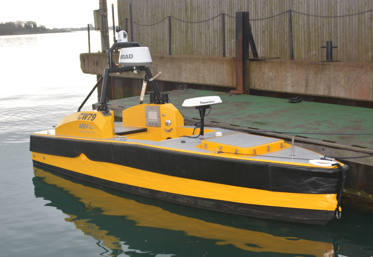
(a) AMV C-Worker 5

(b) AMV physics

Figure 1: An AMV in real and a model of its physics

Indicated in Figure 1b, at time $t\in T$, we consider the velocity $\bm{v}_{A}=[v_{A}^{x},v_{A}^{y}]^{T}$ and position $\bm{p}_{A}$ of the AMV, the position $\bm{p}_{W}$ of a next waypoint to be approached, and a set $O$ of obstacles, each described by its velocity $\bm{v}_{O_{i}}$ and position $\bm{p}_{O_{i}}$. $\bm{p}$ and $\bm{v}$ are vectors in planar coordinates $(x,y)$ over $\mathbb{R}^{2}$. These parameters form a state space $\mathcal{X}$ with tuples

$$\bm{x}=[\bm{p}_{A},\bm{v}_{A},\bm{p}_{O},\bm{v}_{O}]^{T}.$$

Below, we abbreviate $\bm{p}_{E}$ by $E$ where $E\in\{A,O,W\}$. We also consider parameters calculated from $\bm{x}$, such as the distance to the next waypoint $\left\lVert\overline{AW}\right\rVert$ or the angle $\phi_{AO}$ between the AMV velocity vector and the distance vector $\overline{AO}$.

For sake of simplicity, we consider the AMV as a particle with mass $m$ and formulate its dynamics as the following system of ordinary differential equations

$$\dot{\bm{p}}_{A}=\bm{v},\quad\dot{\bm{v}}_{A}=\bm{f}/m,\quad\dot{\bm{v}}_{O}=\bm{0},\quad\text{and}\quad\dot{\bm{p}}_{O}=\bm{0}$$ (1)

where $\bm{f}/m$ implements Newton’s second law of the kinetics of particle masses relating a force applied to the vehicle and this vehicle’s acceleration at time $t$. To remain in scope of our investigation, we further simplify the AMV dynamics, omitting disturbances (e.g. crosswind) and perturbations (e.g. flow resistance), and restricting our analysis to static obstacles.

Modelling the AMV Controller

Figure 2 shows the structure of the plant consisting of the dynamical model of the AMV and its environment (as explained before) and a two-layered controller comprising the AP and the LRE.

Figure 2: Block structure diagram of the dynamical model and the two-layered controller with the corresponding monitors

The discrete low-level control of the vehicle is facilitated by the AP through generating the propulsive force $\bm{f}$ of the AMV as an input to the AMV dynamics. Within the frame of reference of the trajectory of the AMV, we model the AMV’s single thruster by calculating two components of $\bm{f}$, the longitudinal (or tangential) acceleration force $\bm{f}_{l}$ collinear with the AMV’s velocity $\bm{v}$ and the radial acceleration force $\bm{f}_{t}$ perpendicular to $\bm{f}_{l}$, such that

$$\bm{f}=\bm{f}_{l}+\bm{f}_{t}=f_{l}\left[\begin{array}[]{c}\cos(\phi_{A})\\ \sin(\phi_{A})\end{array}\right]+f_{t}\left[\begin{array}[]{c}-\mathrm{sgn}(\phi_{A})\sin(\phi_{A})\\ \mathrm{sgn}(\phi_{A})\cos(\phi_{A})\end{array}\right].$$

The discrete high-level control of the AMV is partially facilitated by the LRE through switching between several operating modes: an OCM, a MOM, a HCM, and a CAM. When in OCM, the operator has responsibility for the AMV. When in MOM, the AMV navigates towards the next waypoint at maximum speed. If it gets close to, but not on collision course with, an obstacle then it switches to HCM. If a potential future collision is detected, it transitions to CAM to make evasive maneuvers. Each of these modes provides the AP with a particular setpoint $\bm{w}=[\mathit{rs},\bm{p}_{W}]^{T}$ (i.e. target speed and location of next waypoint) for the calculation of $\bm{f}$ by the AP as described by the hybrid automaton in Figure 3

$$f_{l} =k_{p}^{l}\cdot|\mathit{rs}-\left\lVert\bm{v}_{A}\right\rVert|$$ (2)

$$f_{t} =\left\{\begin{array}[]{ll}k_{p}^{t}\cdot\phi_{AW},&\text{in MOM}\\ k_{p}^{t}\cdot\mathrm{sgn}(\phi_{AW})\cdot f_{max},&\text{in CAM/HCM}\end{array}\right.$$ (5)

In this example, we use a simple proportional controller for $\bm{f}$ with directional proportionality factors $k_{p}$ as shown in Equations 2 and 2. For obstacle avoidance manoeuvres, we calculate the safe braking distance by

$$d_{sb}=\frac{sb\cdot\left\lVert\bm{v}_{A}\right\rVert^{2}\cdot m}{-2\cdot k_{p}^{b}\cdot f_{max}}$$ (6)

with a safety margin $sb$ to capture modelling uncertainty and define the nO and oCC hazards as the predicates

$$\mathit{nO}\equiv\left\lVert\overline{AO}\right\rVert>d_{sb}\quad\text{and}\quad\mathit{oCC}\equiv\mathit{nO}\mathrel{\wedge}|\phi_{AO}|<\epsilon_{\phi}.$$ (7)

In MOM, we add a hysteresis $\epsilon_{h}$ to $\epsilon_{\phi}$ in order to delay manoeuvre cancellation. Figure 3 describes the overall behaviour of how the LRE switches between the four modes to provide $\bm{w}$ to the AP. From the components LRE and AP shown in Figure 2 and from the modes shown in Figure 3, one can then derive the interfaces for the detailed software design of the AMV control system.

Figure 3: Behaviour of the LRE and AP as a Moore machine $*$…non-deterministic assignment by the operator

Note on Abstraction

The transition from the discrete LRE and AP to the continuous AMV physics is accomplished by a conversion of (D)iscretely timed $\bm{f}$ inputs in form of (C)ontinuous, piece-wise constant signals, processed by actuators. Vice versa, the digital controller (particularly, the Aggregator in Figure 2) samples the environment through sensors at a certain rate. Figure 2 indicates this abstraction by D/C and C/D converters. Although we chose to apply this abstraction to the generation of $\bm{f}$, in practice, this will happen inside the thrusters where, e.g. digital signals control a servo motor of a combustion engine and a rudder to generate $\bm{f}$.

Simulating the Model

We implemented the AMV model in a simple integrator-based simulator in plain GNU/Octave. For that, we derived parameters, such as weight, maximum speed and propulsive force, from the C-Worker 5 specification. Additionally, we identified controller constants, such as $k_{p}^{l}$, during simulation. Figure 4 shows a trajectory of the AMV (green dot) turning around to make its way to the next waypoint $W$ (blue dot) while circumventing a floating obstacle (pink dot). The initial state $\bm{x}_{0}\in\mathcal{X}$ is set to

$$\bm{x}_{0}=[\underbrace{-.5,-3.8}_{\bm{v}_{A}[m/s]},\underbrace{-10,-10}_{\bm{p}_{A}[m]},\underbrace{0,0}_{\bm{v}_{O_{1}}[m/s]},\underbrace{-12,-18}_{\bm{p}_{O_{1}}[m]},\dots]^{T}$$

and the simulation run for the constants $\mathit{rs}=4m/s$, $\bm{p}_{W}=[0,0]^{T}$, and the time interval $T=[0,35]$ sec. Note, the 2D trajectory from the AMV exhibits a deviation from its course where $\mathit{oCC}$ turned true. The lower middle graph shows this as the event of $d_{sb}\approx 13>|\overline{AO}|$ where the magenta curve touches the red curve at $t\approx 5s$, simultaneous to the reduction of $\left\lVert\bm{v}_{A}\right\rVert$ after the switch to $\mathit{CAM}$ (cf. top right graph).

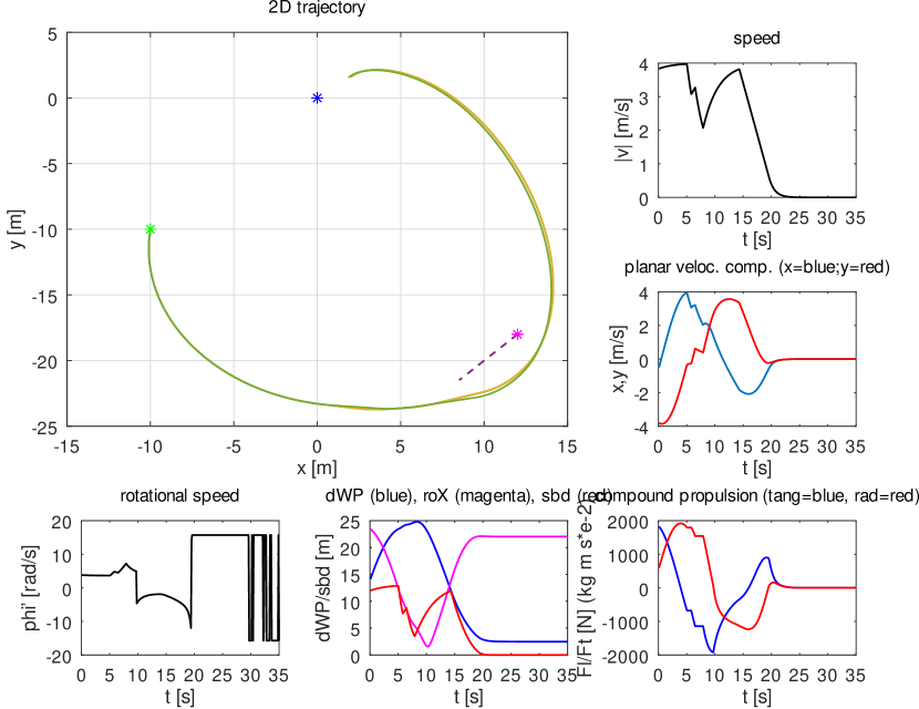
Figure 4: Simulation: the AMV (green dot) approaching next waypoint (blue dot) while crossing an obstacle (pink dot)

Beyond Simulation

Our quest for covering the input space (Section I) requires us to ask how we can know that from wherever in $\mathcal{X}$ we start, wherever an obstacle is, in whatever interval $T$ we evaluate a trajectory, will the AMV always steer away from an obstacle in CAM, will it always reduce speed in HCM, will it reach the next waypoint within a given time in MOM? Such questions require a more fundamental investigation of the model discussed in the next section.

III-B Verification

In order to support deductive verification of AMV, we apply Isabelle/UTP to prove properties of the controller and system dynamics. For this, we utilise Isabelle/$\textsf{d}\mathcal{H}$ which integrates $\textsf{d}\mathcal{H}$ [Munive2018-DDL, Foster2020-dL] into Isabelle/UTP. We extend it with matrices, discrete variables, and modular reasoning. Along with standard Hoare logic laws, Isabelle/$\textsf{d}\mathcal{H}$ includes the key rules from $\textsf{d}\mathcal{L}$, including differential induction and cut, which are at the core of our verification approach. We prove these laws as theorems of Hoare logic in Isabelle/UTP.

Theorem III.1.

Differential Induction and Cut

$$\leavevmode\nobreak\ \leavevmode\nobreak\ \leavevmode\nobreak\ \dfrac{\textit{differentiable}(P)\mathrel{\wedge}(B\Rightarrow\mathcal{L}_{F}(P))}{\left\{P\middle\}\,\langle\dot{\bm{x}}=F(\bm{x})\leavevmode\nobreak\ |\leavevmode\nobreak\ B(\bm{x})\rangle\,\middle\{P\right\}}$$ (8)

$$\dfrac{\left\{P\middle\}\,\langle F\leavevmode\nobreak\ |\leavevmode\nobreak\ B\rangle\,\middle\{P\right\}\leavevmode\nobreak\ \left\{Q\middle\}\,\langle F\leavevmode\nobreak\ |\leavevmode\nobreak\ B\mathrel{\wedge}P\rangle\,\middle\{Q\right\}}{\left\{P\mathrel{\wedge}Q\middle\}\,\langle F\leavevmode\nobreak\ |\leavevmode\nobreak\ B\rangle\,\middle\{Q\right\}}$$ (9)

Here, $\langle\dot{\bm{x}}=F(\bm{x})\leavevmode\nobreak\ |\leavevmode\nobreak\ B(\bm{x})\rangle$ is a system of ODEs with an evolution domain $B$. The dynamical system is permitted to evolve provided that the ODEs in $F$, and predicate $B$, are satisfied for all points on the solution trajectory. (8) states that if $P$ is everywhere differentiable, and its differentiated form follows from $B$, then $P$ is an invariant. (9) shows that if we can prove that $P$ is invariant, then we can use it as an axiom of the dynamics to prove that $Q$ is also an invariant [Platzer2008].

We extend [Foster2020-dL] with support for automation of Lie derivatives [Ghorbal2014-AlgInv] evaluation. The ODEs are encoded as a vector field $F:\mathbb{R}^{n}\to\mathbb{R}^{n}$. $\mathcal{L}_{F}(P)$ denotes the Lie derivative of the predicate $P$ along $F$. $P$ is restricted to the form $e\leavevmode\nobreak\ R\leavevmode\nobreak\ f$, for $R\in\{=,\leq,<\}$, over differentiable expressions $e,f:\mathbb{R}^{n}\to\mathbb{R}$, and their conjunctions and disjunctions, such as $2x\leq 5$. We exemplify $\mathcal{L}$ below.

$$\mathcal{L}_{F}(e\leq f) =(\mathcal{L}_{F}(e)\leq\mathcal{L}_{F}(f))$$ (10)

$$\mathcal{L}_{F}(e+f) =\mathcal{L}_{F}(e)+\mathcal{L}_{F}(f)$$ (11)

$$\mathcal{L}_{F}(e\cdot f) =\mathcal{L}_{F}(e)\cdot f+e\cdot\mathcal{L}_{F}(f)$$ (12)

$$\mathcal{L}_{F}(\sin(e)) =\mathcal{L}_{F}(e)\cdot\cos(e)$$ (13)

$$\mathcal{L}_{F}(x) =(\lambda s:\mathbb{R}^{n}.\,\textit{{get}}_{x}\leavevmode\nobreak\ F(s))$$ (14)

These are largely standard, such as the product rule (12). Of note, (14) shows the treatment of a continuous variable $x:\mathbb{R}$. We encode mutable variables using lenses [Foster07], which are pairs

$$(x:V\Longrightarrow S)\triangleq(\textit{{get}}_{x}:S\to V,\textit{{put}}_{x}:S\to V\to S)$$

for some suitable state space $S$ and variable type $V$, that obey intuitive algebraic laws [Foster2020-IsabelleUTP]. Here, we require that every continuous variable has a bounded linear get function, which is satisfied, for example, when $x$ is a projection of a Euclidean space. The derivative of $x$ is an expression that applies the get function to the derivative of the state ($F(s)$). This can be seen as a semantic substitution of $x$ by its derivative [Foster2020-IsabelleUTP].

Invariants can contain transcendental functions such as $\sin$ and $log$. We also support equalities between arbitrary Euclidean spaces, such as matrices. To close the gap between Octave and Isabelle, we have implemented a smart matrix parser. A matrix in Isabelle is represented by a function: $A\leavevmode\nobreak\ \textit{mat}[M,N]\triangleq N\to M\to A$, where $N$ and $M$ are finite types denoting the dimensions, and $A$ is the element type, usually $\mathbb{R}$. Thus, the Isabelle type system can be used to ensure that matrix expressions are well-formed. We use the syntax

$$\left[[x^{1}_{1},x^{1}_{2},\cdots x^{1}_{n}],\cdots,[x^{m}_{1},x^{m}_{2},\cdots,x^{m}_{n}]\right]$$

to represent a $m$ by $n$ matrix in Isabelle, which is a list of lists. Our parser can infer the dimensions of a well-formed matrix, and produce suitable dimension types, which aids proof. Moreover, we have proved theorems that allow symbolic evaluation of certain vector operations, for example:

$$[x_{1},y_{1}]+[x_{2},y_{2}] =[x_{1}+x_{2},y_{1}+y_{2}]$$

$$n\cdot[x,y] =[n\cdot x,n\cdot y]$$

We also define the matrix lens

$$\textit{mat-lens}(m:M,n:N):A\Longrightarrow A\leavevmode\nobreak\ \textit{mat}[M,N]$$

which accesses an element. With it, we can model both variables that refer to an entire matrix and also its elements.

We have developed a tactic in Isabelle/$\textsf{d}\mathcal{H}$ called dInduct, which automates the application of Theorem III.1 by determining whether $P$ is indeed differentiable everywhere, and if so applying differentiation and substitution. The resulting predicate can be discharged, or refuted, using Isabelle’s tactics.

Hybrid systems in Isabelle/$\textsf{d}\mathcal{H}$ follow the pattern of $Sys\triangleq(Ctrl\mathrel{\hbox{\rm;}}Dyn)^{\star}$, where the controller and dynamics iteratively take turns in updating the variables [Mitsch2017Obstacle]. Proving a safety property $P$ of $Sys$ entails finding an invariant $I$ both of $Ctrl$ and $Dyn$, such that $I\Rightarrow P$. Isabelle/$\textsf{d}\mathcal{H}$ splits the state space of a hybrid system into its continuous and discrete variables. Continuous variables change during evolution, but discrete variables are constant and updated only by assignments.

The continuous state space ($\Sigma_{C}$) must form a Euclidean space, and so is typically composed of reals, vectors, and matrices. There are no restrictions on the discrete state space, and it may use any Isabelle data type.

Case Study

We describe each of the continuous variables using lenses, e.g. $\bm{p},\bm{v}:\mathbb{R}\leavevmode\nobreak\ \textit{mat}[1,2]\Longrightarrow\Sigma_{C}$. In addition to those mentioned in §III-A, we also include $\bm{a}:\mathbb{R}\leavevmode\nobreak\ \textit{mat}[1,2]$ for the acceleration, and $s:\mathbb{R}$, for the linear speed. Technically, $s$ can be derived as $\left\lVert v\right\rVert$, but its inclusion makes proving invariants easier. Most are monitored variables of the environment, except $\bm{a}$, which is updated by the AP. The discrete variables include waypoint location ($\bm{wp}:\mathbb{R}^{2}$); obstacle set ($ob:\mathbb{P}(\mathbb{R}^{2})$); linear speed and heading set points ($rs,rh:\mathbb{R}$); force vector ($\bm{f}:\mathbb{R}^{2}$); and mode ($m:\{\textit{OCM},\textit{MOM},\textit{HCM},\textit{CAM}\}$). Next, we describe the dynamics.

Definition III.2 (AMV Dynamics).

$$dyn_{AV} \triangleq\left(\begin{array}[]{l}\dot{t}=1;\ \dot{\bm{p}}=\bm{v};\ \dot{\bm{v}}=\bm{a};\ \dot{\bm{a}}=0;\\ \dot{s}=\dfrac{\bm{v}\cdot\bm{a}}{s}\mathop{\hbox{\raisebox{0.0pt}{$\leftslice$}}}s\neq 0\mathop{\hbox{\raisebox{0.0pt}{$\rightslice$}}}\left\lVert\bm{a}\right\rVert;\\ \dot{\phi}=acos\left(\dfrac{(\bm{v}+\bm{a})\cdot\bm{v}}{\left\lVert\bm{v}+\bm{a}\right\rVert\cdot\left\lVert\bm{v}\right\rVert}\right)\mathop{\hbox{\raisebox{0.0pt}{$\leftslice$}}}s\neq 0\mathop{\hbox{\raisebox{0.0pt}{$\rightslice$}}}0\end{array}\right)$$

$$ax_{AV} \triangleq\left(\begin{array}[]{l}0\leq s\mathrel{\wedge}s\leq S\mathrel{\wedge}s\cdot\begin{bmatrix}\sin(\phi)\\ \cos(\phi)\end{bmatrix}=\bm{v}\mathrel{\wedge}t<\epsilon\end{array}\right)$$

$$Dyn \triangleq t:=0\mathrel{\hbox{\rm;}}\left\langle dyn_{AV}\leavevmode\nobreak\ |\leavevmode\nobreak\ ax_{AV}\right\rangle$$

Dynamics $dyn_{AV}$ is a system of six ODEs. For the linear speed derivative, we consider the special case when $s=0$, where the speed derivative is derived from $\bm{a}$, and the rotational speed is 0. We also axiomatise some properties of the dynamics in $ax_{AV}$: (1) the linear speed must be in $[0,S]$; (2) $\bm{v}$ must be the same as $s$ multiplied by the orientation unit vector; (3) time must not advance beyond $\epsilon$, which puts an upper bound on the time between control decisions.

Next, we model the LRE, which is encoded as a set of guarded commands derived from Figure 3. In each iteration, the LRE updates state variables and can transition to a different state. Whilst in MOM, the speed set point is the maximum speed (S), and the LRE invokes the command steerToWP that updates the heading towards the current way point.

Definition III.3 (Simplified LRE).

$LRE\triangleq$

$$\left(\begin{array}[]{l}m=\textit{MOM}\rightarrow\left(\!\begin{array}[]{l}rs:=S\mathrel{\hbox{\rm;}}\textit{steerToWP}\mathrel{\hbox{\rm;}}\\ \textbf{if}\leavevmode\nobreak\ \textit{oCC}\leavevmode\nobreak\ \textbf{then}\leavevmode\nobreak\ m:=\textit{CAM}\leavevmode\nobreak\ \textbf{fi}\mathrel{\hbox{\rm;}}\\ \textbf{if}\leavevmode\nobreak\ \exists\bm{o}\in ob.\left\lVert\bm{o}-\bm{p}\right\rVert\leq D\\ \textbf{then}\leavevmode\nobreak\ m:=\textit{HCM}\mathrel{\hbox{\rm;}}rs:=H\leavevmode\nobreak\ \textbf{fi}\end{array}\right)\\[12.91663pt] m=\textit{HCM}\rightarrow\left(\begin{array}[]{l}rs:=H\mathrel{\hbox{\rm;}}\textit{steerToWP}\mathrel{\hbox{\rm;}}\\ \textbf{if}\leavevmode\nobreak\ \forall\bm{o}\in ob.\left\lVert\bm{o}-\bm{p}\right\rVert>D\\ \textbf{then}\leavevmode\nobreak\ m:=\textit{MOM}\leavevmode\nobreak\ \textbf{fi}\end{array}\right)\\[12.91663pt] m=\textit{OCM}\rightarrow\textbf{skip}\\ m=\textit{CAM}\rightarrow\cdots\end{array}\!\right)$$

If oCC is detected the LRE transitions to CAM. If nO holds but not oCC, then the LRE switches to HCM. From HCM, the speed set point is decreased to $H$. Once the AMV is no longer close to an obstacle, the LRE may return to MOM. OCM exhibits no behaviour since the operator provides the control inputs. Finally, CAM is where collision avoidance procedures are executed. Its behaviour is left unspecified for now. The final component we model is the AP.

Definition III.4 (Autopilot Controller).

$AP\triangleq$

$$\begin{array}[]{l}\textbf{if}\left\lVert rs-s\right\rVert>s_{\epsilon}\\ \textbf{then}\leavevmode\nobreak\ ft:=\mathrm{sgn}(rs-s)\cdot\min\left(\!\begin{array}[]{c}kp_{gv}\cdot\left\lVert rs-s\right\rVert,\\ f_{max}\end{array}\!\right)\\ \textbf{else}\leavevmode\nobreak\ ft:=0\leavevmode\nobreak\ \textbf{fi}\mathrel{\hbox{\rm;}}\\ \textbf{if}\left\lVert rh-\phi\right\rVert>\phi_{\epsilon}\\ \textbf{then}\leavevmode\nobreak\ fl:=\mathrm{sgn}(rh-\phi)\cdot\min\left(\!\begin{array}[]{c}kp_{gr}\cdot\left\lVert rh-\phi\right\rVert,\\ f_{max}\end{array}\!\right)\\ \textbf{else}\leavevmode\nobreak\ fl:=0\leavevmode\nobreak\ \textbf{fi}\mathrel{\hbox{\rm;}}\\ \bm{f}:=fl\cdot\begin{bmatrix}\cos(\phi)\\ \sin(\phi)\end{bmatrix}+ft\cdot\begin{bmatrix}\sin(\phi)\\ \cos(\phi)\end{bmatrix}\mathrel{\hbox{\rm;}}\bm{a}:=\bm{f}/m\end{array}$$

The AP takes $rs$ and $rh$ as inputs, computes $\bm{f}$, and calculates $\bm{a}$. The constants $s_{\epsilon}$ and $\phi_{\epsilon}$ limit the controller activity when the speed is close to the set point. Its representation in Isabelle/UTP is shown in Figure 5. Continuous variables are distinguished using the namespace $\mathbf{c}$, e.g. $\textbf{c}{:}x$. Scalar multiplication and division are distinguished operators, $n*_{R}\bm{x}$ and $n\mathop{/_{R}}\bm{x}$. Finally, we describe the overall AMV behaviour.

Figure 5: Autopilot in Isabelle/UTP

Definition III.5.

$AMV\triangleq(LRE\mathrel{\hbox{\rm;}}AP\mathrel{\hbox{\rm;}}Dyn)^{\star}$

The LRE executes first to determine the new speed set points. Following this, the autopilot calculates the new acceleration vector. Finally, the dynamical system evolves the continuous variables for up to $\epsilon$ seconds, and then the cycle begins again. We will now proceed to verify some properties of the system using Isabelle/$\textsf{d}\mathcal{H}$. We begin with some structural properties.

Theorem III.6 (Structural Properties).

• $LRE\mathop{\,\textit{{nmods}}\,}\{t,\bm{p},\bm{v},\bm{a},s,\phi\}$

• $AP\mathop{\,\textit{{nmods}}\,}\{t,\bm{p},\bm{v},s,\phi\}$

• $Dyn\mathop{\,\textit{{nmods}}\,}\{\bm{wp},ob,rs,rh,ft,fl,\bm{f},m\}$

$P\mathop{\,\textit{{nmods}}\,}A$ means that $P$ does not modify the variables in $A$. It enables modular verification using the following theorem:

$$S\mathop{\,\textit{{nmods}}\,}\bm{x}\implies\left\{p(\bm{x})\middle\}\,S\,\middle\{p(\bm{x})\right\}$$

If $\bm{x}$ is not modified by $S$, then any predicate in $\bm{x}$ is invariant. We can verify that the LRE does not modify any of the continuous variables, as it only updates the (discrete) set points. The AP modifies only the continuous variable $\bm{a}$. We can prove that $ax_{AV}$ is an invariant of both $LRE$ and $AP$, and therefore of the entire system. The dynamics can potentially change any of the continuous variables, but does not change any of the discrete variables. These structural properties are automatically proved, and are useful to ensure structural well-formedness of a controller under development.

We next prove some invariants of the system using $\textsf{d}\mathcal{H}$.

Theorem III.7 (Collinearity of $\bm{v}$ and $\bm{a}$).

$$\left\{\bm{a}\cdot\bm{v}=\left\lVert\bm{a}\right\rVert\cdot\left\lVert\bm{v}\right\rVert\middle\}\,Dyn\,\middle\{\bm{a}\cdot\bm{v}=\left\lVert\bm{a}\right\rVert\cdot\left\lVert\bm{v}\right\rVert\right\}$$

Proof.

We first prove that $\bm{a}\cdot\bm{v}\geq 0$ and $(\bm{a}\cdot\bm{v})^{2}=(\bm{a}\cdot\bm{a})\cdot(\bm{v}\cdot\bm{v})$ are both invariants by theorem III.1. We can then show these are equivalent with $a\cdot v=\left\lVert\bm{a}\right\rVert\cdot\left\lVert\bm{v}\right\rVert$. ∎

Collinearity means that $\bm{v}$ and $\bm{a}$ have the same direction and the AMV is travelling straight. A corollary is below.

$$\left\{\!\bm{a}\cdot\bm{v}=\left\lVert\bm{a}\right\rVert\!\cdot\!\left\lVert\bm{v}\right\rVert\!\middle\}\,Dyn\,\middle\{\bm{p}=\frac{t^{2}}{2}\cdot\bm{a}+t\cdot old(\bm{v})+old(\bm{p})\right\}$$

This states that if the AMV is travelling in a straight line, then its position can be obtained through integration of $\dot{\bm{p}}$. By Theorem III.6, collinearity is also trivially an invariant of the $LRE$, since it does not modify any continuous variables.

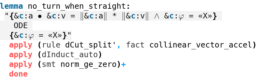
Figure 6: Example proof in Isabelle/$\textsf{d}\mathcal{H}$

We show proof of a further corollary in Figure 6 in Isabelle/UTP: if the AMV is moving straight, then the heading is constant. We introduce a ghost variable $X$ for the current heading $\phi$. The proof proceeds by performing a differential cut (dCut_split’), which allows us to assume collinearity in the dynamical system. Theorem III.7 corresponds to the fact collinear_vector_accel in Isabelle. Then, we use differential induction via the dInduct_auto tactic, which also applies algebraic simplification laws. Finally, we call sledgehammer which provides SMT proofs to discharge the remaining proof obligation, which is essentially $\bm{a}\cdot\bm{v}=\left\lVert\bm{a}\right\rVert\!\cdot\!\left\lVert\bm{v}\right\rVert\Rightarrow\dot{\phi}=0$. This technique allows us to harness all the mathematical results proved in HOL and HOL-Analysis in our proofs [Harrison2005-Euclidean, Immler2012].

Collinearity is established by $AP$ when the heading set point is the same as the actual heading:

Theorem III.8 (Autopilot Collinearity).

$$\left\{\begin{array}[]{c}0\leq s\mathrel{\wedge}s\leq rs\\ \mathrel{\wedge}\left\lVert rh-\phi\right\rVert<\phi_{\epsilon}\\ \mathrel{\wedge}\bm{v}=s\cdot\begin{bmatrix}\sin(\phi)\\ \cos(\phi)\end{bmatrix}\end{array}\middle\}\,AP\,\middle\{\bm{a}\cdot\bm{v}=\left\lVert\bm{a}\right\rVert\cdot\left\lVert\bm{v}\right\rVert\right\}$$

Proof.

Hoare logic reasoning and vector arithmetic. A crucial fact is that $[\sin(\phi),\cos(\phi)]\cdot[\sin(\phi),\cos(\phi)]=1$. ∎

The theorem shows that if the linear speed is between 0 and $rs$, $\phi$ and $rh$ are sufficiently close, and $\bm{v}$ can be derived from the linear speed and heading, then afterwards $\bm{a}$ and $\bm{v}$ are again collinear. Now, by the sequential composition law, we can compose this with III.7 to obtain the same Hoare triple for $AP\mathrel{\hbox{\rm;}}Dyn$. Finally, we show a property of the LRE.

$$\left\{\!\begin{array}[]{c}m=MOM\mathrel{\wedge}\\ \left\lVert\textit{ang}(\bm{wp}-\bm{p})-\phi\right\rVert\leq\phi_{\epsilon}\\ \mathrel{\wedge}(\exists\bm{o}\in ob.\left\lVert\bm{p}-\bm{o}\right\rVert\leq D)\end{array}\!\middle\}\,LRE\,\middle\{\!\begin{array}[]{c}m=HCM\\ \mathrel{\wedge}rs=H\mathrel{\wedge}\\ \left\lVert rh-\phi\right\rVert\leq\phi_{\epsilon}\end{array}\!\right\}$$

This shows that if the LRE is in MOM, and the heading is currently towards the waypoint, but an obstacle is close, then it will transition to HCM, drop the set point speed to $H$ and the requested heading remains close to the actual heading.

IV Discussion and Conclusion

In this paper, we have made preliminary steps to integrating NC with theorem proving in Isabelle. Octave and Isabelle’s approaches to mathematics are, in many ways, quite different. Octave is focused on efficient NC, whereas Isabelle is based on foundational mathematics and proof. Nevertheless, our investigation indicates that they can effectively be used together.

Most of the required Octave functions, such as, $\sin$, $\mathrm{sgn}$, and the vector operations are present in Isabelle, and are accompanied by a large body of theorems [Harrison2005-Euclidean, Immler2012, Immler2014]. The Archive of Formal Proofs (AFP) has several useful libraries; for example, we used Manuel Eberl’s library for calculating angles [Triangle-AFP]. Combining libraries with the flexible syntax of Isabelle, the program notation of Isabelle/UTP, and our matrix syntax, we can achieve a fairly direct translation of Octave functions, as Figure 5 illustrates. Verification can be automated by the hoare-auto tactic, though this dependends on arithmetic lemma libraries, some of which we needed to prove manually for the verification. Nevertheless, in our experience, sledgehammer [Blanchette2011] performs quite well with arithmetic problems. Moreover, Isabelle has the approximation tactic, which can prove real and transcendental inequalities [Holzl2009-Approximate].

For the dynamics, it is necessary to produce an explicit system of first order ODEs, as shown in Definition III.2. Consequently, any algebraic equations must be converted. For example, we could not include the value of $\phi$, but needed to give its derivative and include an axiom linking this with $s$ and $\bm{v}$. The challenge is finding invariants, and having sufficient background lemmas to prove the verification conditions.

There have been previous works on integrating NC with deductive verification. Notably, Zhan et al.  [Zou2013-HHL] have used Hybrid CSP and an accompanying Hoare logic to verify Simulink block diagrams in Isabelle. Our work is more modest, in that we focus on sequential hybrid programs, but with a transparent translation and a high degree of automation. The dominant and most automated tool for hybrid systems deductive verification remains KeYmaera X [KeYmaeraX, Mitsch2017Obstacle]. Nevertheless, we believe that our preliminary results show the advantages of targeting Isabelle. Firstly, this allows integration of a variety of mathematical libraries to support reasoning. Secondly, we can combine notations with ODEs, and in the future aim to support refinement to code using libraries like Isabelle/C [Tuong2019-CIsabelle]. Thirdly, as illustrated by the obstacle register, with Isabelle/HOL we have the potential to extend $\textsf{d}\mathcal{L}$ with additional features like collections as used in quantified $\textsf{d}\mathcal{L}$ [Platzer2010-qDL].