Dynamical response and competing orders in two-band Hubbard model

Abstract

We present a dynamical mean-field study of two-particle dynamical response functions in two-band Hubbard model across several phase transitions. We observe that the transition between the excitonic condensate and spin-state ordered state is continuous with a narrow strip of supersolid phase separating the two. Approaching transition from the excitonic condensate is announced by softening of the excitonic mode at the $M$ point of the Brillouin zone. Inside the spin-state ordered phase there is a magnetically ordered state with $2\times 2$ periodicity, which has no precursor in the normal phase.

I Introduction

Spontaneous symmetry breaking, which accompanies the continuous phase transitions, changes qualitatively the dynamical response of solids. If the broken symmetry is continuous, low-energy Goldstone mode(s) associated with the long-wavelength dynamics of the order parameter, appears in systems with short-range interactions. Excitonic condensates (ECs) Mott (1961); Keldysh and Kopaev (1965); Halperin and Rice (1968) represent an exotic type of broken-symmetry phase. While the experimental realizations of EC has been limited to artificial structures such as quantum wells in strong magnetic field Eisenstein and MacDonald (2004) or cavity systems Balili et al. (2007), recent experiments on 1T-TiSe₂ Cercellier et al. (2007); Kogar et al. (2017) , Ca₂RuO₄ Jain et al. (2017) or Pr_0.5Ca_0.5CoO₃ Tsubouchi et al. (2002); Moyoshi et al. (2018) revived the interest in the subject also in bulk solids. Condensation of spinful excitons, which gives rise to a new type of magnetic behavior is particularly interesting. The simplest model to capture the excitonic magnetism is the two-orbital Hubbard model at half filling Kuneš and Augustinský (2014); Hoshino and Werner (2016); Kaneko and Ohta (2014) and its strong-coupling limit Khaliullin (2013); Nasu et al. (2016); Tatsuno et al. (2016). The parameter range of interest hosts a number of ordered phases Kuneš (2015); Nasu et al. (2016) in addition to the first-order metal-insulator transition Werner and Millis (2007). Besides the general interest in understanding its behavior, the model provides a fertile playground for testing theoretical methods.

Computation of two-particle (2P) response for realistic materials is a challenging task. Dynamical mean-field theory (DMFT) Georges et al. (1996); Kotliar et al. (2006) has been successful in bringing together the material realism of multi-orbital models with the many-body realism, including real temperatures, phase transitions, quasi-particle life times, atomic-multiplet effects. Despite the boom of the past two decades, application of DMFT has been largely limited to one-particle (1P) quantities, such as generalized band structures and occupation numbers. Solved in principle, the calculation of 2P response functions is numerically very demanding as it involves the solution of the Bethe-Salpeter equation for large multi-index objects. There are compelling reasons to study the 2P response within DMFT. Most experimental probes and applications employ the 2P response of materials. Current density functional methods do not allow even approximate access to dynamical susceptibilities of correlated materials. The static susceptibilities are essential to ensure the stability of the obtained solutions.

In this paper we study the dynamical susceptibilities of the two-orbital Hubbard model on a bipartite lattice at half filling. In particular, we focus on the mechanism of transition between the EC and spin-state order (SSO) phases. The studied phase transitions involve both continuous and discrete symmetry breaking and multi-atomic unit cells. Besides understanding the physics of the model and assessing the performance of the method, this work is the next step towards similar investigations within the LDA+DMFT framework for real materials.

II Computational Method

The studied model Hamiltonian reads

$$\begin{split}H=&\sum_{<ij>,\sigma}(t_{a}a_{i\sigma}^{\dagger}a_{j\sigma}+t_{b}b_{i\sigma}^{\dagger}b_{j\sigma})+H.c.\\ &+\frac{\Delta}{2}\sum_{i,\sigma}(n^{a}_{i\sigma}-n^{b}_{i\sigma})\\ &+U\sum_{i,\alpha}n^{\alpha}_{i\uparrow}n^{\alpha}_{i\downarrow}+\sum_{i,\sigma\sigma^{\prime}}(U^{\prime}-J\delta_{\sigma\sigma^{\prime}})n^{a}_{i\sigma}n^{b}_{i\sigma^{\prime}},\end{split}$$ (1)

where $a^{{\dagger}}_{i\sigma}$ and $b^{{\dagger}}_{i\sigma}$ are the fermionic creation operators for electrons in the respective orbitals $a$ and $b$, with spin $\sigma$, at site $i$ of a square lattice. The first term describes nearest neighbor hopping. The remaining terms, containing the particle number operators $n^{c}_{i,\sigma}\equiv c^{{\dagger}}_{i\sigma}c_{i\sigma}$, correspond to the crystal-field $\Delta$, the Hubbard interaction $U$, and Hund’s exchange $J$ in the Ising approximation. The values $U=4$, $J=1$, and $U^{\prime}=U-2J$ are fixed throughout this study. The remaining parameters $t_{a}$, $t_{b}$, $\Delta$ as well as the temperature $T$ are varied. All calculations reported here are performed for the filling of two electrons per atom.

We follow the standard DMFT procedure, in which the lattice model is mapped onto an auxiliary Anderson impurity model (AIM) Georges and Kotliar (1992); Jarrell (1992). The AIM is solved numerically, using the ALPS implementation Bauer et al. (2011); Shinaoka et al. (2017); Gaenko et al. (2017) of the matrix version of the strong-coupling continuous-time quantum Monte-Carlo (CT-QMC) algorithm Werner et al. (2006).

The model hosts several competing phases, which can be distinguished by the mean values of operators

$$\begin{split}\phi_{i}^{\gamma}&=R_{i}^{\gamma}+iI_{i}^{\gamma}=\sum_{\alpha\beta}\sigma^{\gamma}_{\alpha\beta}a_{i\alpha}^{\dagger}b_{i\beta}^{\phantom{\dagger}}\\ O_{i}&=\sum_{\sigma}(n^{a}_{i\sigma}-n^{b}_{i\sigma})\\ S_{i}^{z}&=\sum_{c=a,b}(n^{c}_{i\uparrow}-n^{c}_{i\downarrow}).\end{split}$$ (2)

Here $\phi_{i}^{\gamma}$, with the Hermitean and anti-Hermitean parts $R_{i}^{\gamma}$ and $iI_{i}^{\gamma}$, creates an $S=1$ exciton on site $i$. The $\sigma^{\gamma}$ ($\gamma=x,y,z$) are Pauli matrices, which represent the spin polarization of the exciton. With the density-density form of the interaction, which mimics an easy-axis single-ion anisotropy, $\langle\phi_{i}^{z}\rangle=0$ applies throughout the studied parameter range Kuneš (2015). The $O_{i}$ and $S_{i}^{z}$ represent the local orbital polarization and the $z$-component of the spin moment, respectively.

The susceptibilities $\chi^{X}(\mathbf{k},\omega)$ are obtained by analytic continuation Gubernatis et al. (1991); Geffroy et al. (2019) of their Matsubara representations

$$\chi^{X}(\mathbf{k},i\nu_{n})=\!\!\int_{0}^{\beta}\!\!\!\!\!\mathrm{d}\tau e^{i\nu_{n}\tau}\expectationvalue{X_{-\mathbf{k}}(\tau)X_{\mathbf{k}}(0)}-|\expectationvalue{X_{\mathbf{k}}}|^{2}\\$$ (3)

where the Fourier transform is defined as $X_{\mathbf{k}}=\frac{1}{\sqrt{N}}\sum_{\mathbf{R}}e^{-i\mathbf{k}\cdot\mathbf{R}}X_{\mathbf{R}}$. The observables $X$ of interest are represented by the operators listed in (2).

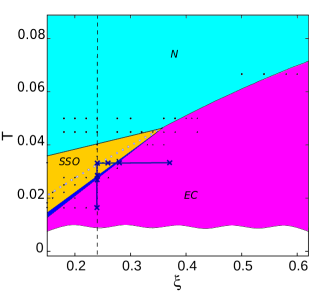
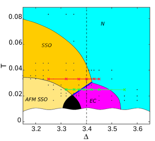
Figure 1: Cuts through the phase diagram of the studied model along the $\xi$–$T$ ($\Delta=3.4$, top) and $\Delta$–$T$ ($\xi=0.24$, bottom) planes. Black symbols mark the parameters for which a calculation was performed. The dashed vertical line is common to both panels. The narrow blue wedge separating the EC and SSO phases represents the SS phase. The red, blue and violet cuts with crosses mark the points for which the susceptibilities are analyzed in Figs. 4, 5 and 6, respectively. Open blue circles in the left panel were taken from Ref. Kuneš and Augustinský, 2014 and indicate instability of the normal (N) phase towards EC. The black wedge separating the AFM SSO and EC phases in the right panel indicate a putative coexistence regime accompanying a first order transition. (Actual calculations investigating this transition were not performed).

We start with the 1P propagators at 300 Matsubara frequencies to obtain the bare susceptibilities (both local and lattice bubble terms), which are then transformed into the Legendre polynomial representation Boehnke et al. (2011). The 2P correlation function is sampled using the CT-QMC algorithm. The local 2P-irreducible vertex $\Gamma$ is obtained by inverting the impurity Bethe-Salpeter equation (BSE) Georges et al. (1996); Kuneš (2011); van Loon et al. (2015); Krien et al. (2017). Using this vertex to solve the lattice BSE, we obtain the lattice correlation functions. This procedure is performed independently for each bosonic Matsubara frequency. We have found that using 10 bosonic frequencies allows for a stable and good quality analytic continuation. We use between 22 (for the zeroth bosonic frequency) and 30 Legendre coefficients (for the ninth bosonic frequency). A sizable reduction of the computational and storage cost can be achieved with the procedure of Ref. Otsuki et al., 2017; Shinaoka et al., 2020.

The susceptibility $\chi^{X}(\mathbf{k},i\nu_{n})$ is a diagonal element of the particle-hole susceptibility matrix $\bm{\chi}(\mathbf{k},i\nu_{n})$ obtained by summation of the lattice correlation function over the Legendre coefficients. The matrix $\bm{\chi}(\mathbf{k},i\nu_{n})$ is indexed by pairs of flavors (spin/orbital/site) inside the unit cell, while the inter-cell structure is diagonalized by going to the reciprocal space. With four flavors per site, $\bm{\chi}(\mathbf{k},i\nu_{n})$ has dimension $4^{2}$ for 1-atom cell. In phases with 2-atom cells $\bm{\chi}(\mathbf{k},i\nu_{n})$ has the dimension $(2\times 4)^{2}$. However, thanks to the locality of the 2P-irreducible vertices, the BSE can be written in a closed form for elements of the type $\chi_{ii,jj}$, where $i$, $j$ are the site indices. Therefore the diagonal elements in (3) can be obtained by working with matrices of the flavor dimension $2\times 4^{2}$, i.e., linear in the number of sites per the unit cell.

To ensure comparability of $\chi^{X}(\mathbf{k},i\nu_{n})$ in different phases (various unit cells) we present all susceptibilities (3) in the large Brillouin zone of the 1-atom unit cell. In the phases with 1-atom unit cell the susceptibility is diagonal in $\mathbf{k}$. In phases with $\sqrt{2}\times\sqrt{2}$ 2-atom unit cells there are no-zero off-diagonal elements connecting $\mathbf{k}$ and $\mathbf{k}+(\pi,\pi)$. The transformation from the 2-atom unit cell, in which the BSE inversion is performed, is given by

$$\begin{split}\chi(\mathbf{k})&=\tilde{\chi}(\mathbf{k}^{\prime})_{11,11}+\tilde{\chi}(\mathbf{k}^{\prime})_{22,22}\\ &+\exp(ik_{y})\tilde{\chi}(\mathbf{k}^{\prime})_{11,22}+\exp(-ik_{y})\tilde{\chi}(\mathbf{k}^{\prime})_{22,11},\end{split}$$ (4)

where $\tilde{\chi}$ and $\mathbf{k}^{\prime}\equiv(k^{\prime}_{x},k^{\prime}_{y})=(k_{y}-k_{x},k_{y}+k_{x})$ are related to the 2-atom unit cell. The subscripts of $\tilde{\chi}$ refer to the two sites in the 2-atom unit cell (The orbital and spin indices are not shown for sake of simplicity).

III Results and Discussion

A Phase diagram and order parameters

In Fig. 1 we show the phase diagram of the model in the $\xi$–$T$ plane of band asymmetry parameter $\xi=\frac{2t_{a}t_{b}}{t_{a}^{2}+t_{b}^{2}}$ and temperature $T$ at fixed crystal field $\Delta$, and in the $\Delta$–$T$ plane at fixed $\xi$. The phase boundaries are obtained by combination of the calculated order parameters and diverging susceptibilities. The phase diagram in Fig. 1a generalizes that of Ref. Kuneš and Augustinský, 2014 to the ordered phases. The phase diagram in Fig. 1b should be compared to the phase diagrams of related strong-coupling models in Refs. Kuneš, 2015; Tatsuno et al., 2016. Unlike previous studies Kuneš and Augustinský (2014); Hoshino and Werner (2016) where the instabilities of the normal phase were investigated, here we perform linear response calculations also in the thermodynamically stable ordered phases. Four distinct ordered phases are identified.

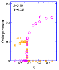
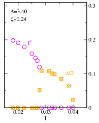
Figure 2: The order parameters: staggered orbital polarization $\Delta O$ and the uniform excitonic-condensate amplitude $\langle I^{y}\rangle$ along the cuts in the phase diagram Fig. 1 marked by the frame colors.

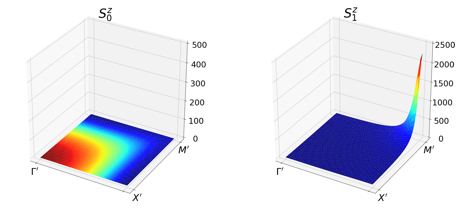
Figure 3: Site resolved static susceptibility $\chi^{S^{z}}(\mathbf{k}^{\prime})$ for $T=0.0333$, $\xi$=0.24, $\Delta$ =3.23 in the SSO phase. It describes the response to a field applied only on the LS-like sublattice (left) and on the HS-like sublattice (right). The reciprocal vector $\mathbf{k}^{\prime}$ is expressed with respect to the 2-atom unit cell.

Polar excitonic condensate (EC). This phase was analyzed in detail in a number of previous studies Kuneš (2014); Kuneš and Geffroy (2016); Geffroy et al. (2018); Nasu et al. (2016); Kaneko and Ohta (2014). It is characterized by a finite expectation value of $\langle\bm{\phi}_{i}\rangle=\bm{\phi}$, which fulfills the condition ${\bm{\phi}^{*}\times\bm{\phi}=0}$ Balents (2000); Geffroy et al. (2018). The EC phase preserves the translation symmetry, but breaks two continuous $U(1)$ symmetries associated with the global conservation of $\sum_{i}S_{i}^{z}$ and $\sum_{i}O_{i}$. The EC order parameter ’lives’ on a $T_{2}$ torus - it can pick an arbitrary orientation in the spin $xy$-plane and an arbitrary complex phase. Throughout the present study we fix its orientation to $\langle I^{y}\rangle\neq 0$, while the other components are zero.

Spin state order (SS0). The SSO phase in the two-band Hubbard model was reported in Ref. Kuneš, 2011 and in multi-orbital material specific DMFT studies Karolak et al. (2015); Afonso et al. (2019). It was proposed as an explanation of high field experiments on LaCoO₃ Altarawneh et al. (2012); Ikeda et al. (2016). It is characterized by staggered orbital polarization $\Delta O=(-1)^{i}\langle O_{i}-\bar{O}\rangle$, where $(-1)^{i}$ describes the $\sqrt{2}\times\sqrt{2}$ order and $\bar{O}$ denotes an average over all lattice sites. The SSO is a strong-coupling effect that, unlike the EC phase, does not have a weak-coupling analog Kuneš and Augustinský (2014). At $T=0$ the phase is a checkerboard arrangement of LS and HS sites. In the studied parameter range the LS-like sites are dominated by the LS state with a negligible HS contribution. The population of the HS state on HS-like sites is only up to 60%, with the remainder being predominantly LS states . The SSO phase breaks the translation symmetry, but the continuous $U(1)$ symmetries associated with $S^{z}$ and $O$ conservation are preserved.

Supersolid (SS). The SS phase is characterized by the simultaneous appearance of the EC and SSO orders Boninsegni and Prokof’ev (2012); Scalettar et al. (1995). The SS phase breaks all the symmetries broken by EC and SSO phases. We consistently find very narrow strip of the SS phase at the boundary between the EC and SSO phases, see Fig. 2.

Antiferromagnetic spin state order (AFM-SSO). The SSO phase has a large residual entropy associated with the spin disorder on the HS sites. The nearest neighbor AFM exchange interaction on the HS sublattice (3rd neighbor interaction on the original lattice) leads to a $2\times 2$ order consisting in checkerboard spin order on the HS sublattice. We did not actually perform calculations in the AFM SSO phase, but determined the SSO/AFM-SSO phase boundary as the divergence of $\tilde{\chi}^{S^{z}}(M^{\prime},0)$, see Fig. 3.

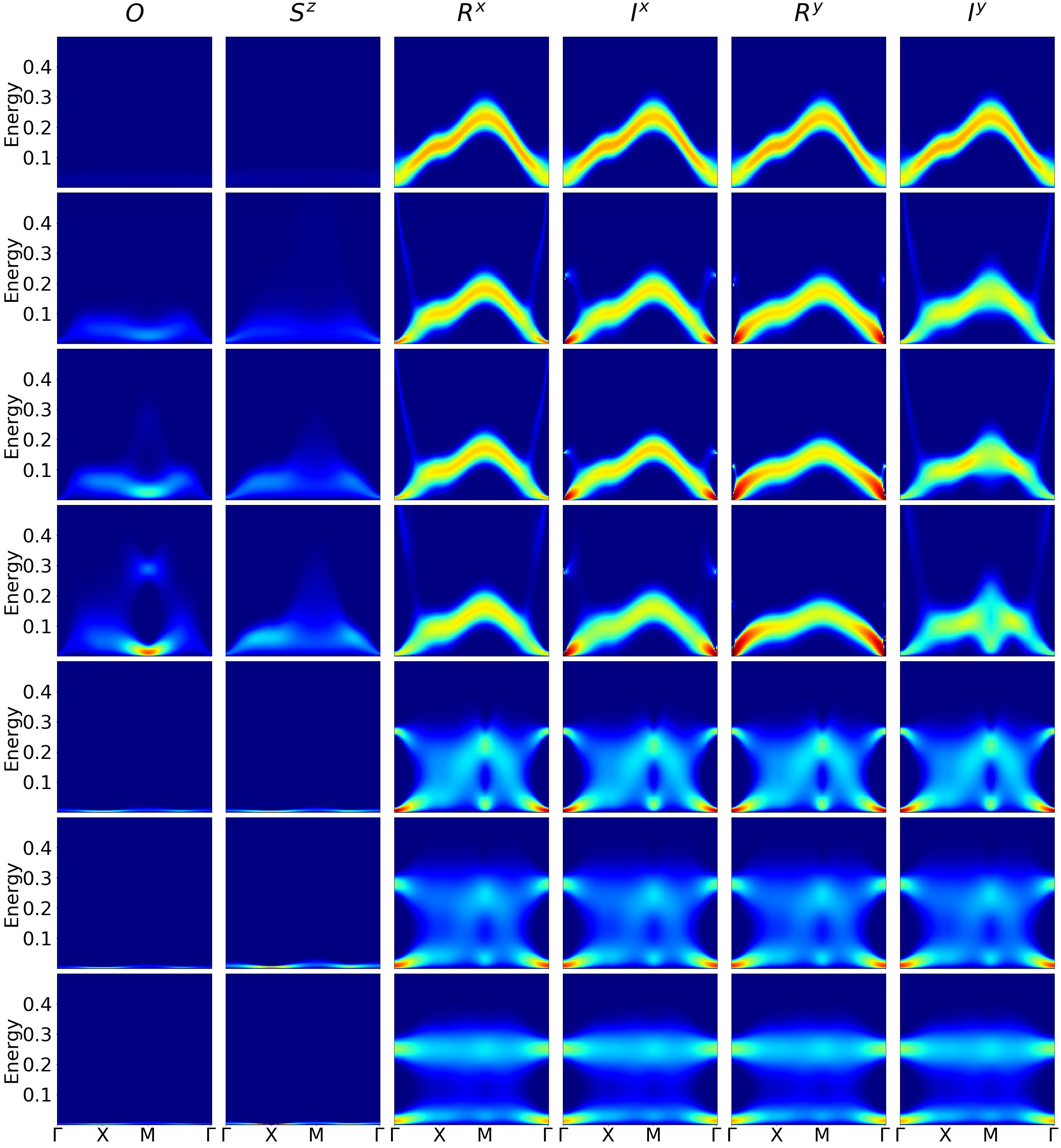
Figure 4: Evolution of the dynamical susceptibility $\chi^{X}(\mathbf{k},\omega)$ with the crystal field $\Delta$ along the green line ($\xi=0.24$, $T=0.025$) in Fig. 1b. The columns correspond to different Hermitean operators $X$, the rows correspond to different $\Delta$: 1) $\Delta=3.55$ normal phase, 2–4) $\Delta=3.45$, 3.42, 3.39 EC phase, 5–7) $\Delta=3.37$, 3.35, 3.32 SSO phase. The color coding represents the spectral density $B(\mathbf{k},\omega)=-\frac{1}{\pi}\operatorname{Im}\chi^{X}(\mathbf{k},\omega)$. In order to capture the entire dispersion in the presence of divergent density of the Goldstone modes we introduce a cut-off and plot $\frac{B}{B+\text{const}}$ with const=5.5. Note that in the SSO phase there is a large intensity of $\chi^{S^{z}}$ at $\omega\approx 0$ (difficult to see in the present figures) corresponding to large static response of local moments on HS sites.

B Dynamical susceptibility

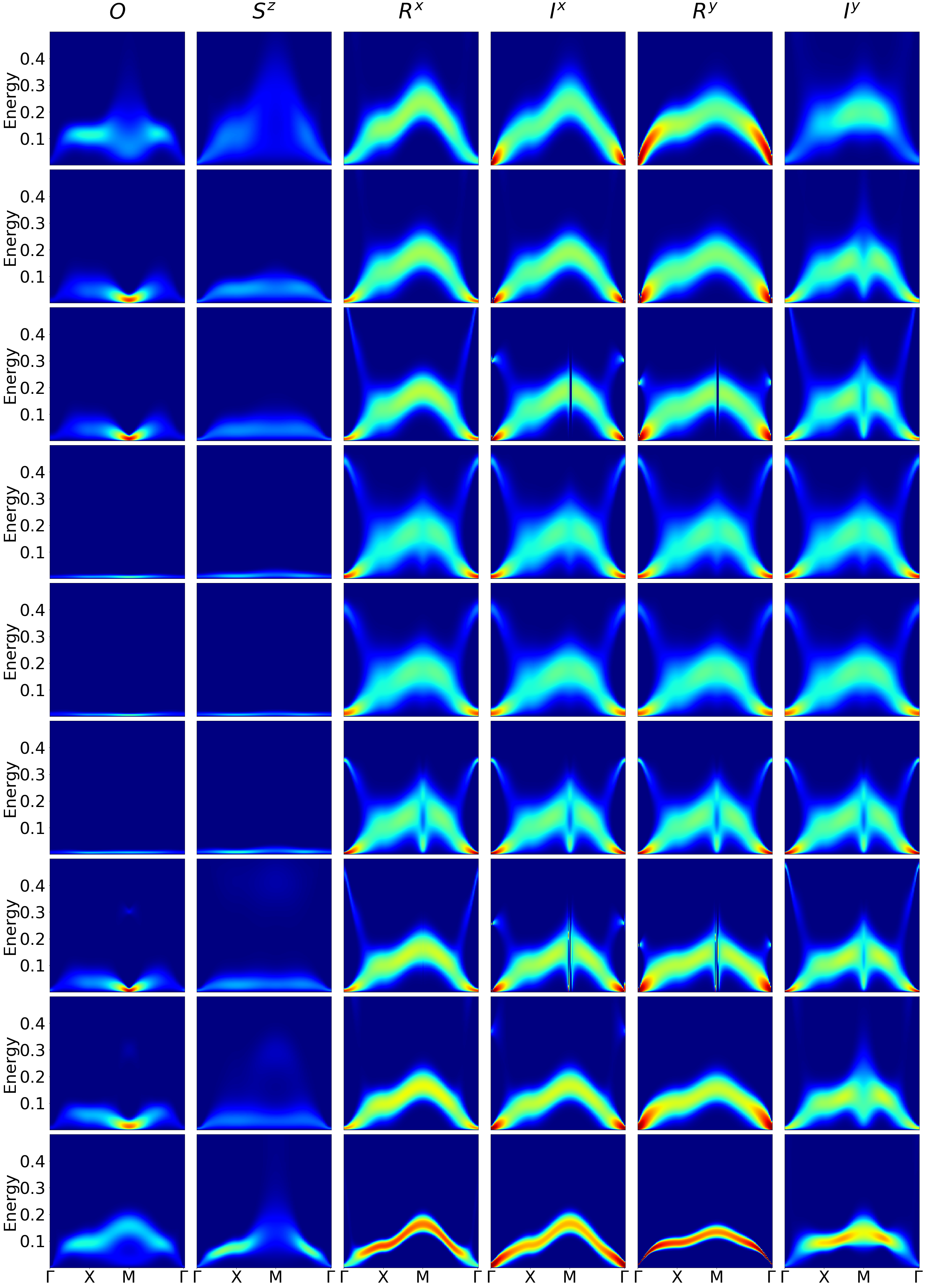
Figure 5: As in Fig. 4, evolution of the dynamical susceptibility $\chi^{X}(\mathbf{k},\omega)$ along the inverted L-shaped blue line in Fig. 1a for $\Delta$ = 3.4. The horizontal line corresponds to fixed temperature $T=0.033$, while the vertical line corresponds to fixed band asymmetry $\xi=0.24$. The rows correspond to different parameters: rows 1–2) $\xi=0.37$, 0.30; EC phase, 3) $\xi=0.278$; SS phase, 4–5) $\xi=0.26$, 0.24; SSO phase, 6) $T=0.0286$; SSO phase, 7) $T=0.0278$; SS phase, 8–9) $T=0.0370$, 0.0167; EC phase.

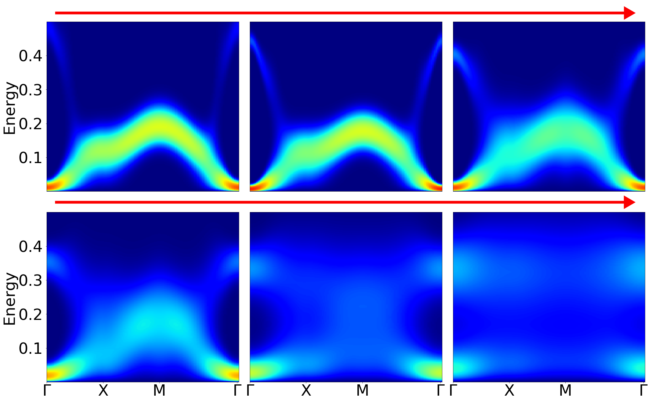
Figure 6: Evolution of the dynamical excitonic susceptibility $\chi^{X}(\mathbf{k},\omega)$ with crystal field $\Delta$ along the red line($\xi$=0.24, $T=0.0333$) in Fig. 1b.1–2) $\Delta=3.45$, 3.42; normal phase, 3–6) $\Delta$ = 3.40, 3.37, 3.32, 3.27; SSO phase.

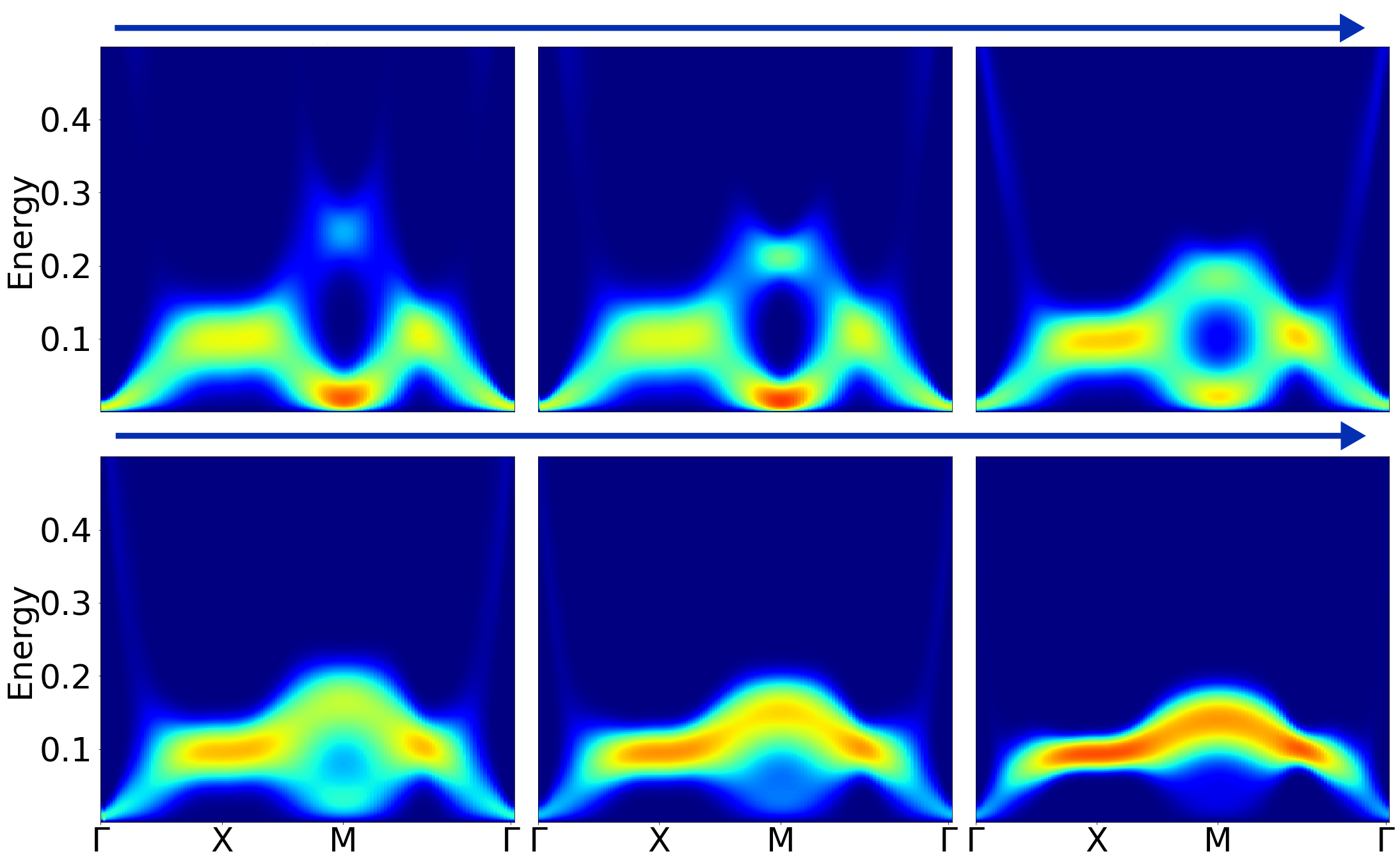
Figure 7: Dynamical susceptibility $\chi^{\tilde{I}^{y}}(\mathbf{k},\omega)$ in the EC phase of Fig. 5 ($\Delta=3.40$; $\xi$=0.24; $T=0.0270$, 0.02632, 0.025, 0.0222, 0.02, 0.0167 in the order marked by the arrow) in the basis of the eigenmodes of the static susceptibility.

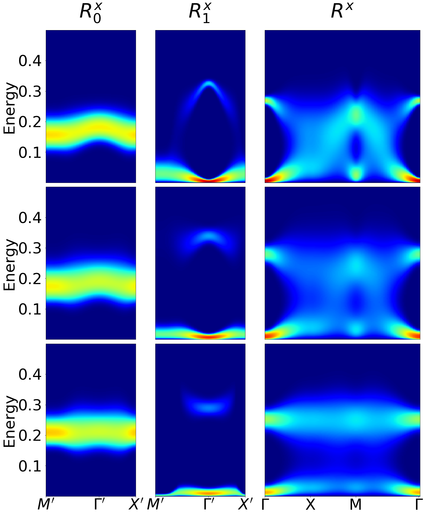
Figure 8: Dynamical excitonic susceptibilities $\chi^{X}(\mathbf{k},\omega)$ in the SSO phase of Fig. 4 ($T=0.025$; $\Delta=$3.37, 3.35, 3.32 from top to bottom) in the basis of the eigenmodes of the static susceptibility. The $R^{x}_{0}$ and $R^{x}_{1}$ columns refer to the two eigenmodes in the 2-atom unit cell of the SSO. The $k$-path refers to the Brillouin zone for the 2-atom unit cell. The $R^{x}$ column reproduces the data from Fig. 4 for comparison ($k$-path in the Brillouin zone of 1-atom unit cell).

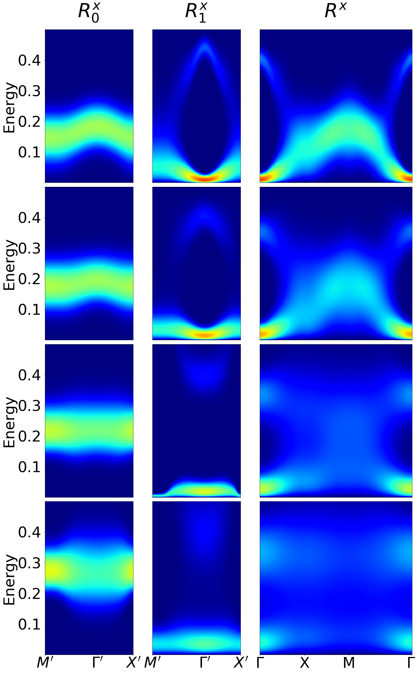
Figure 9: Dynamical excitonic susceptibilities $\chi^{T}(\mathbf{k},\omega)$ in the SSO phase of Fig. 6 ($T=0.0333$; $\Delta=3.4$, 3.37, 3.32, 3.25 from top to bottom) in the basis of the eigenmodes of the static susceptibility. The notation is the same as in Fig. 8.

The main focus of this work is the behavior of the dynamical susceptibility across the transition between the EC and SSO states. In Fig. 4 we show the evolution of $\chi^{X}(\mathbf{k},\omega)$ ($X$=$O$, $S^{z}$, $R^{x}$, $I^{x}$, $R^{y}$, $I^{y}$) along the $\Gamma$-X-M-$\Gamma$ path in the 2D Brillouin zone with increasing crystal fields $\Delta$.

First, we review the discussion of the N–EC transition from Ref. Geffroy et al., 2019. The normal (N) phase is characterized by gapped excitonic dispersion, reflected in all excitonic susceptibilities. The equivalence of $x$ and $y$ elements originates from the $S^{z}$-conservation, while the equivalence of $R$ and $I$ elements originates from the $O$-conservation. The $O$- and $S^{z}$-susceptibilities exhibit no dynamics (non-zero only for $\nu_{n}=0$) and vanish at low temperature. Reducing $\Delta$ results in closing of the excitonic gap and eventually transition to the EC phase, where the equivalence of excitonic susceptibilities is broken. Deep in the EC phase we can distinguish $x$ and $y$ excitonic modes with distinct dispersion. The corresponding susceptibilities $R_{x}$, $I_{x}$ and $R_{y}$, $I_{y}$ follow these dispersions, but have vastly different amplitudes at low energies. The $I^{x}$ and $R^{y}$ exhibit linear dispersion and diverging amplitudes at $\Gamma$, reflecting the spin-rotation and phase-rotation Goldstone modes Geffroy et al. (2019).

The $S^{z}$- and $O$-susceptibilities acquire non-zero dynamics due to the $S^{z}$–$R^{x}$ and $O$–$I^{y}$ coupling in the EC phase. The induced dynamics of $S^{z}$ was explained in terms of the strong-coupling model in Ref. Geffroy et al., 2019, see also SM SM . The dynamical response of $O$ can be understood along similar lines. In the strong coupling limit $O_{i}$ maps onto the number operator of excitons ${O_{i}=d_{ix}^{\dagger}d_{ix}^{\phantom{\dagger}}+d_{iy}^{\dagger}d_{iy}^{\phantom{\dagger}}}$. Replacing $d_{iy}^{\dagger}$ with $i\tfrac{\phi}{2}+d_{iy}^{\dagger}$ in the EC phase we find ${O_{i}\sim-\tfrac{\phi}{2}(d_{iy}^{\dagger}-d_{iy}^{\phantom{\dagger}})}$, and thus the correlation function of $O$ follows that of $I^{y}$. For a more rigorous derivation see SM SM . We point out that all the above identifications are understood relative to the orientation of the EC order parameter: $\langle I^{y}\rangle\neq 0$.

As we near the SSO phase the behavior of the $O$, $S_{z}$ and $I_{y}$ susceptibilities changes qualitatively. The $O$ and $S_{z}$ dynamics cease to be slave to the excitonic dynamics and their dispersions stop to follow the excitonic ones. Similar behavior is observed as we approach the phase boundary as a function of crystal field $\Delta$, Fig. 4, band asymmetry $\xi$ or temperature $T$, Fig. 5. The $O$ susceptibility develops a hot spot at the $M$ point, a precursor of the SSO phase, which is accompanied by softening of $\chi^{I}_{y}$ at $M$. Similar behavior at the $M$ point was previously observed at zero temperature for spinless hard-core bosons on square lattice and interpreted as roton excitations known from superfluid helium Scalettar et al. (1995). We provide the strong-coupling mean-field analysis of the softening and EC–SSO transition in the Supplemental Material SM .

The demise of the EC phase due to the softening of the excitonic mode accompanied by the divergence of ${\chi^{O}(\mathbf{k}=M,0)}$ opens the possibility for a continuous transition between the EC and SSO phases via an intermediate SS phase. Indeed, we find several solutions with both EC and SSO order, Fig. 2, which fall into an narrow strip of parameters. We point out that a similar situation was found in Ref. Scalettar et al., 1995.

In the SSO phase, we observe the remains of broad excitonic dispersion in the vicinity of the phase boundary. It is important to point out that at the studied temperatures, the LS sites host almost exclusively the LS state, but the HS sites host still up to 75% LS and only 25% HS states Kuneš (2011). Proceeding deeper into the SSO phase the excitonic dispersion gives way to two almost flat bands. These can be associated with creation of an exciton (LS to HS transition) on the LS site (upper band) and annihilation of an exciton (HS to LS transition) on the HS site (lower band).

C Mode analysis

The connection between dynamical susceptibilities in Figs. 4, 5 and 6 on the one hand, and bosonic dispersions obtained in the strong coupling model SM ; Scalettar et al. (1995); Nasu et al. (2016) on the other hand, is not straightforward. In the strong-coupling limit and at $T=0$, the susceptibilities follow the dispersions of the $d_{x}$ or $d_{y}$ bosons with intensity depending on the specific correlation function. Our model is not in the strong-coupling limit and partly falls into a high temperature regime. The bosonic modes, a 2P basis in which $\bm{\chi}(\mathbf{k},\omega)$ is diagonal , are not immediately obvious.

We attempt to obtain approximate modes by diagonalizing the static susceptibility $\bm{\chi}(\mathbf{k},\omega=0)$. This procedure is trivial in the normal phase, because each of the four mutually equal excitonic susceptibilities forms a diagonal block of $\bm{\chi}(\mathbf{k},\omega)$. In the SSO phase the excitonic susceptibilities do not mix with other elements of $\bm{\chi}(\mathbf{k},\omega)$ or with each other, and the diagonalization is reduced to $2\times 2$ blocks spanned by the two sites of the 2-atom unit cell.

The dominant effect of diagonalization in the EC phase is to combine $I^{y}$ with $O$ into a single low-energy mode with large spectral weight $\tilde{I}^{y}$. In Fig. 7, we show the evolution of $\chi^{\tilde{I}^{y}}(\mathbf{k},\omega)$ as we approach the EC/SS phase boundary by varying the temperature along the cut analyzed in Fig. 5. Deep in the EC phase, $\chi^{\tilde{I}^{y}}$ is essentially identical to $\chi^{{I}^{y}}$. As we get closer to the phase boundary, a mode softening at the $M$-point is clearly observable. Interestingly, it does not proceed as a smooth deformation of the dispersion curve captured by the strong-coupling model SM , but rather through a spectral weight transfer between the upper and low branch of the O-ring structure observed at $T$=0.025. We attribute this behavior to the finite temperature.

In Figs. 8, 9, we show the mode decomposition in the SSO phase. For all parameters we find two bands reminiscent of the strong-coupling behavior Scalettar et al. (1995); Nasu et al. (2016). Deep in the SSO phase the bands are flat. The lower one corresponds to eliminating a HS exciton on the nominally HS sublattice. The upper band corresponds to creating a HS exciton on the nominally LS sublattice. With increasing crystal field $\Delta$, the character of the bands changes and they become dispersive, while the gap between them shrinks. This behavior is somewhat counter-intuitive, since the difference of HS and LS energies in an isolated atom follows an opposite trend. The explanation lies with the nearest-neighbor repulsion between HS excitons. Increasing $\Delta$ causes a decrease in concentration of HS states on the nominally HS sublattice, which reduces the HS-HS repulsion that has to be overcome when creating a HS exciton on the nominally LS sublattice. Simultaneously, a minute shift of the lower excitonic band leads to a condensation as the SSO/SS boundary is approached. At the SSO/N boundary, Fig. 9, the temperature is too high for the excitons to condense. We observe a complete closing of the gap between the two bands, which become a back-folded image of the excitonic band from the 1-atom unit cell. In addition to the two main bands, we observe a weak high-energy feature around the $\Gamma^{\prime}$-point, which does not have a strong-coupling $T=0$ counterpart. This feature exhibits a rather strong dispersion and it is most pronounced close to the boundary of SSO with either the SS or normal phases, Figs. 8, 9 .

IV Conclusions

We have studied the dynamical susceptibility across several phase transitions in the two-orbital Hubbard model using DMFT. We have observed a narrow slip of supersolid phase separating the spin-state order from the excitonic condensate. Approaching the spin-state ordered phase from the exciton condensate is heralded by the softening of a specific collective mode at the $M$-point of the Brillouin zone, identified as the roton instability in Ref. Scalettar et al., 1995. At low temperatures the spin-state ordered phase removes the spin degeneracy by developing antiferromagnetic order with $2\times 2$ periodicity.

The present calculations demonstrate the utility of linear response DMFT formalism for understanding complicated phase diagrams and phase transitions involving the breaking of both discrete and continuous symmetries. While the DMFT susceptibilities in the studied parameter range qualitatively agree with the strong-coupling generalized spin-wave treatment Scalettar et al. (1995); Nasu et al. (2016); SM , they contain features that are beyond this description. Last but not least, we have shown that the symmetry breaking in the exciton condensate gives rise to dynamical response in the spin- and orbital-density channels. These may be studied by standard experimental probes such as inelastic x-ray or neutron scattering, which do not couple directly to the spin-triplet excitonic channel.