Multi-Particle Simulation Techniques

Abstract

The nonlinear space-charge effects play an important role in high intensity/high brightness accelerators. These effects can be self-consistently studied using multi-particle simulations. In this lecture, we will discuss the particle-in-cell method and the symplectic tracking model for self-consistent multi-particle simulations.

1 Introduction

The nonlinear space-charge effects from charged particle Coulomb interactions within a bunched beam present a strong limit on beam intensity in high intensity/high brightness accelerators by causing beam emittance growth, halo formation, and even particle losses. To model the details of beam distribution evolution, in the presence of strong space-charge effects, one needs to solve the full Poisson-Vlasov equations self-consistently. The Poisson-Vlasov equations can be solved using a phase space grid-based method or a multi-particle particle-in-cell (PIC) method. The grid-based method is effective in one or two dimensions [1]; but for the three-dimensional system with six phase space variables, the grid-based method will require an enormous amount of memory even for a coarse grid. Also, the grid-based method may break down when very-small-scale structures form in the phase space. The particle-in-cell model is an efficient method to handle the space-charge effects self-consistently. It has a much lower storage requirement and will not break down even when the phase space structure falls below the grid resolution. It uses a computational grid to obtain the charge density distribution from a finite number of macroparticles and solves the Poisson equation on the grid at each time step. The computational cost is linearly proportional to the number of macroparticles, which makes the simulation fast for many applications. With the advance of computers, the PIC method has been implemented on high performance parallel computers for large scale beam dynamics simulation. The parallel PIC also provides a means of reducing fluctuations by enabling use of more particles and of improving spatial resolution through increased grid density. It also dramatically reduces the computation time. The PIC method has been widely used to study the dynamics of high intensity/high brightness beams in accelerators [2, 3, 4, 5, 6, 7, 8, 9, 10, 11, 12, 13, 14, 15, 16, 17].

2 Particle-in-cell method for self-consistent multi-particle simulation

In the particle-in-cell method, a number of macroparticles (i.e. simulation particles with the same charge-to-mass ratio as the real charged particle) are generated from the Monte-Carlo sampling of a given initial distribution in phase space. The trajectories of these charged macroparticles are tracked subject to both the external fields from the accelerating and focusing elements in the accelerator and from the self-consistent space-charge fields due to the Coulomb interactions among the charged particles.

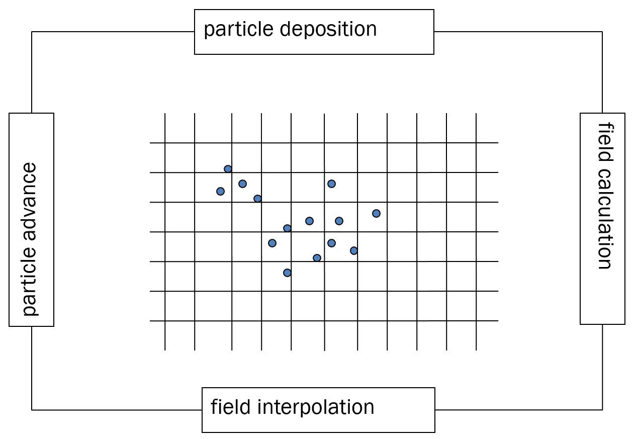
Figure 1: A schematic plot of a single step loop in the particle-in-cell beam dynamics simulation.

Fig. 1 shows a schematic plot of a single step loop in the PIC beam dynamics simulation. It includes four stages: particle advance, charge deposition, self-consistent field calculation on mesh grid, and field interpolation. The particle deposition stage and the field interpolation stage are two symmetric stages that provide the information exchange between the point-like particle and the computational grid. Before the charge deposition, the particle coordinates are transformed into the moving beam frame from the laboratory frame using the relativistic Lorentz transformation. After the field interpolation, the fields are transformed back to the laboratory frame for particle momentum advance. The field calculation stage solves the Poisson equation and calculates the space-charge fields using the charge density distribution on the grid in the beam frame. The particle advance stage updates the particle position and momentum using the space-charge fields and the external fields. In some numerical integrators such as the leap-frog integrator, the update of the position and the update of the momentum can be done at separate sub-step locations within a step [18]. This single step loop is repeated for a number of times in the accelerator beam dynamics simulation. In the following subsections, we will discuss these sub-steps in details.

2.1 Particle deposition and field interpolation

In the PIC method, the self-consistent space-charge fields are calculated on a spatial grid using the charge density distribution on the grid at every dynamically evolving step. The density distribution on the grid is given by:

$$\rho_{p}(x_{p}) = \sum_{i}q_{i}w_{dep}(x_{i}-x_{p})$$ (1)

where $\rho_{p}$ is the charge density on the spatial grid $p$, $q_{i}$ is the charge of the macroparticle $i$, $w_{dep}$ is the weight function for deposition, $x_{i}$ is the spatial coordinates of particle $i$, and $x_{p}$ is the grid coordinate. The solved space-charge fields on the grid are interpolated back to the macroparticle position for momentum update. This is given by:

$${\bf E}_{i} = \sum_{p}{\bf E}_{p}w_{int}(x_{i}-x_{p})$$ (2)

where ${\bf E}_{i}$ is the electric field at the $i^{th}$ macroparticle location, ${\bf E}_{p}$ is the electric field at the grid point $p$, and $w_{int}$ is the interpolation weight function from the grid point $p$ to the particle point $i$. The use of the grid in the PIC method reduces the computational cost of the space-charge field calculation compared with the direct point-to-point calculation that scales as the square of the number of marcroparticles. The cost of field calculation depends on the number of grid points, which is normally much less than the number of macroparticles. The use of grid also provides smoothness to the shot noise and close collision in the direct particle-to-particle calculation. From Eq. 1, by averaging the weighted charge of individual macroparticle, the charge density distribution on the grid is smoother than the original particle distribution. Meanwhile, the interactions among individual particles become the interactions among spatial grid points. In order to control the errors introduced in the deposition/interpolation stage, one should choose the weight function so that the field error is small when the particle separations is large compared with the mesh grid spacing. Also, the charge assigned to the mesh from a particle and the field interpolated to a particle from the mesh should vary smoothly as the particle moves across the mesh. In many applications, in order to avoid the self-force from a single particle on itself, the same weight function for the deposition and the interpolation is used in the PIC method, i.e. $w_{dep}=w_{int}$. Two most widely used weight functions are the linear cloud-in-cell (CIC) and the quadratic triangular shaped cloud (TSC) functions [19, 20]. The weight function for the CIC is given as:

$$w_{p}(x) = 1-|\frac{x-x_{p}}{h}|$$ (3)

and

$$w_{p}(x) = \left\{\begin{array}[]{ll}\frac{3}{4}-(\frac{x-x_{p}}{h})^{2},&|x-x_{p}|\leq h/2\\ \frac{1}{2}(\frac{3}{2}-\frac{|x-x_{p}|}{h})^{2},&h/2<|x-x_{p}|\leq 3/2h\\ 0&{\rm otherwise}\end{array}\right.$$ (7)

for the TSC weight function. A schematic plot of those functions in one dimension are shown in Fig. 2. The linear CIC weight function involves two grid points in one dimension. This weight function maintains the field continuity across the grid points. The quadratic TSC function involves three grid points in one dimension. The first derivative of the field value will be continuous using this weight function. The higher order weight function can be constructed from the convolution of the lower order weight function with the square nearest-grid-point weighting function (also called top-hat function). The higher order weight function is, the smoother the density function will be, and the more computational cost it will take.

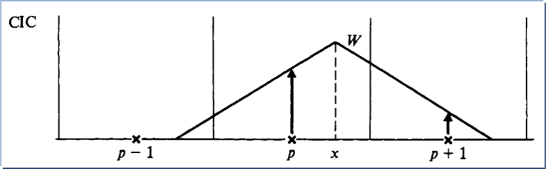
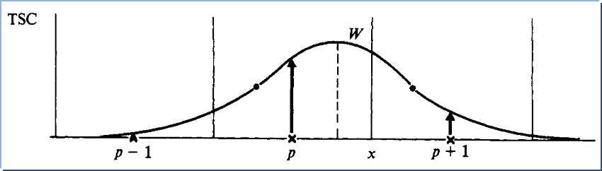
Figure 2: The CIC weight function (left) and the TSC weight function (right) used in charge density deposition [19].

2.2 Poisson solvers for space-charge field calculation

Using the charge density on the grid, one can solve the Poisson equation subject to appropriate boundary conditions in the beam frame to attain the self-consistent space-charge fields at each step. In order to achieve reasonable simulation return time for practical applications that involve thousands and even millions evolution steps, the Poisson solver needs to be fast and computationally efficient. Here, an efficient algorithm refers to the algorithm whose computational cost scales linearly $(O(N))$ or log-linearly $(O(Nlog(N))$ with respect to the number of unknowns to be solved. Under different boundary conditions, different numerical algorithms should be used to solve the Poisson equation effectively. In this lecture, we focus on two types of boundary conditions: one is the open boundary condition, and the other is the finite domain boundary condition.

2.2.1 FFT based Green’s function method for the open boundary condition

The solution of the Poisson equation can be written as:

$$\phi(x,y,z) = \frac{1}{4\pi\epsilon_{0}}\int G(x,x^{\prime},y,y^{\prime},z,z^{\prime})\rho(x^{\prime},y^{\prime},z^{\prime})\ dx^{\prime}dy^{\prime}dz^{\prime}$$ (8)

where $G$ is Green’s function of the Poisson equation, $\rho$ is the charge density distribution function. For a beam inside an accelerator, the pipe aperture size is normally much larger than the transverse size of the beam. In this case, an open boundary condition can be assumed for the solution of the Green’s function in the above equation. Here, the Green function is given by:

$$G(x,{x}^{\prime},y,{y}^{\prime},z,{z}^{\prime}) = \frac{1}{\sqrt{(x-{x}^{\prime})^{2}+(y-{y}^{\prime})^{2}+(z-{z}^{\prime})^{2}}}$$ (9)

Now consider a simulation of an open system where the computational domain containing the particles has a range of $(0,L_{x})$, $(0,L_{y})$ and $(0,L_{z})$, and where each dimension is discretized using $N_{x}$, $N_{y}$ and $N_{z}$ point, from Eq. 8, the electric potentials on the grid can be approximated as:

$${\phi}(x_{i},y_{j},z_{k}) = \frac{h_{x}h_{y}h_{z}}{4\pi\epsilon_{0}}\sum_{i^{\prime}=1}^{N_{x}}\sum_{j^{\prime}=1}^{N_{y}}\sum_{k^{\prime}=1}^{N_{z}}G(x_{i}-x_{i^{\prime}},y_{j}-y_{j^{\prime}},z_{k}-z_{k^{\prime}}){\rho}(x_{i^{\prime}},y_{j^{\prime}},z_{k^{\prime}})$$ (10)

where $x_{i}=(i-1)h_{x}$, $y_{j}=(j-1)h_{y}$, and $z_{k}=(k-1)h_{z}$. The direct numerical summation of the above equation for all grid points can be very expensive and the computational cost scales as $N^{2}$, where $N=N_{x}N_{y}N_{z}$ is the total number of grid points. Fortunately, this summation can be replaced by a summation in a periodic doubled computational domain. Fig. 3 shows an illustrative plot of the doubled computational domain in one-dimensional case.

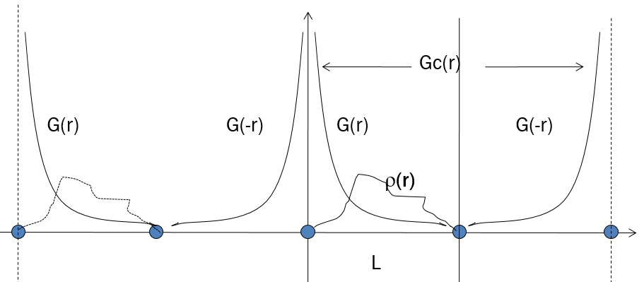
Figure 3: A schematic plot of doubled computational domain in one-dimensional case.

In this periodic doubled computational domain, the original Green’s function in the negative domain, i.e. $G(-r)$, is mapped to the extended domain following the periodic condition. The charge density in the extended domain is set to zero. In this periodic system with a new periodic Green’s function and charge density, the summation can be done efficiently using the FFT method whose computational cost scales as O(Nlog(N)). This new summation yields exactly the same values as the original summation inside the original domain.

In the three-dimensional case, the cyclic convolution is given by [14]:

$${\phi}_{c}(x_{i},y_{j},z_{k}) = \frac{h_{x}h_{y}h_{z}}{4\pi\epsilon_{0}}\sum_{i^{\prime}=1}^{2N_{x}}\sum_{j^{\prime}=1}^{2N_{y}}\sum_{k^{\prime}=1}^{2N_{z}}G_{c}(x_{i}-x_{i^{\prime}},y_{j}-y_{j^{\prime}},z_{k}-z_{k^{\prime}}){\rho}_{c}(x_{i^{\prime}},y_{j^{\prime}},z_{k^{\prime}})$$ (11)

where $i=1,\cdots,2N_{x}$, $j=1,\cdots,2N_{y}$, $k=1,\cdots,2N_{z}$ and

$${\rho}_{c}(x_{i},y_{j},z_{k}) = \left\{\begin{array}[]{r@{\quad:\quad}l}{\rho}(x_{i},y_{j},z_{k})&1\leq i\leq N_{x};\ 1\leq j\leq N_{y};\ 1\leq k\leq N_{z}\\ 0&N_{x}<i\leq 2N_{x}\ or~{}\ N_{y}<j\leq 2N_{y}\ or~{}\ N_{z}<k\leq 2N_{z}\end{array}\right.$$ (14)

$$G_{c}(x_{i},y_{j},z_{k}) = \left\{\begin{array}[]{r@{\quad:\quad}l}G(x_{i},y_{j},z_{k})&1\leq i\leq N_{x}+1;\ 1\leq j\leq N_{y}+1;\ 1\leq k\leq N_{z}+1\\ G(x_{2N_{x}-i+2},y_{j},z_{k})&N_{x}+1<i\leq 2N_{x};\ 1\leq j\leq N_{y}+1;\ 1\leq k\leq N_{z}+1\\ G(x_{i},y_{2N_{y}-j+2},z_{k})&1\leq i\leq N_{x}+1;\ N_{y}+1<j\leq 2N_{y};\ 1\leq k\leq N_{z}+1\\ G(x_{2N_{x}-i+2},y_{2N_{y}-j+2},z_{k})&N_{x}+1<i\leq 2N_{x};\ N_{y}+1<j\leq 2N_{y};\ 1\leq k\leq N_{z}+1\\ G(x_{i},y_{j},z_{2N_{z}-k+2})&1\leq i\leq N_{x}+1;\ 1\leq j\leq N_{y}+1;N_{z}+1<k\leq 2N_{z}\\ G(x_{2N_{x}-i+2},y_{j},z_{2N_{z}-k+2})&N_{x}+1<i\leq 2N_{x};\ 1\leq j\leq N_{y}+1;N_{z}+1<k\leq 2N_{z}\\ G(x_{i},y_{2N_{y}-j+2},z_{2N_{z}-k+2})&1\leq i\leq N_{x}+1;\ N_{y}+1<j\leq 2N_{y};N_{z}+1<k\leq 2N_{z}\\ G(x_{2N_{x}-i+2},y_{2N_{y}-j+2},z_{2N_{z}-k+2})&N_{x}+1<i\leq 2N_{x};\ N_{y}+1<j\leq 2N_{y};N_{z}+1<k\leq 2N_{z}\\ \end{array}\right.$$ (23)

$${\rho}_{c}(x_{i},y_{j},z_{k}) = {\rho}_{c}(x_{i}+2(L_{x}+h_{x}),y_{j}+2(L_{y}+h_{y}),z_{k}+2(L_{z}+h_{z}))$$ (24)

$$G_{c}(x_{i},y_{j},z_{k}) = G_{c}(x_{i}+2(L_{x}+h_{x}),y_{j}+2(L_{y}+h_{y}),z_{k}+2(L_{z}+h_{z}))\ .$$ (25)

These equations make use of the symmetry of the Green function in Eq. 9. From the above definition, one can show that the cyclic convolution gives the same electric potential as the convolution Eq. 10 within the original domain, i.e.

$${\phi}(x_{i},y_{j},z_{k}) = {\phi}_{c}(x_{i},y_{j},z_{k})\hskip 28.45274ptfor~{}\ i=1,N_{x};\ j=1,N_{y};\ k=1,N_{z}\ .$$ (26)

The potential outside the original domain is incorrect but is irrelevant to the original physical domain. Since now both $G_{c}$ and ${\rho}_{c}$ are periodic functions, the convolution for ${\phi}_{c}$ in Eq. 11 can be computed efficiently using the FFT method.

In the above algorithm, both the Green function and the charge density distribution are discretized on the grid. For a beam with aspect ratio close to one, this algorithm works well. However, in some applications, for example, during the emission of electrons out of the cathode, the beam can have a very large transverse to longitudinal ratio. The typical transverse size is on the order of millimeters while the longitudinal size can be about a few tens to hundred microns. Under this situation, the direct use of the Green function on grid point is not efficient since it requires a large number of grid points along the transverse direction in order to get sufficient resolution for the Green function along that direction. If we assume that the charge density function is uniform within each cell centered at the grid point $(x_{i},y_{j},z_{k})$, we can define an effective Green function as:

$${\bar{G}}_{(}x_{i}-x_{i^{\prime}},y_{j}-y_{j^{\prime}},z_{k}-z_{k^{\prime}}) = \int_{x_{i^{\prime}}-h_{x}/2}^{x_{i^{\prime}}+h_{x}/2}dx^{\prime}\int_{y_{j^{\prime}}-h_{y}/2}^{y_{j^{\prime}}+h_{y}/2}dy^{\prime}\int_{z_{k^{\prime}}-h_{z}/2}^{z_{k^{\prime}}+h_{z}/2}dz^{\prime}G(x_{i}-x^{\prime},y_{j}-y^{\prime},z_{k}-z^{\prime})$$ (27)

This integral can be calculated analytically in a closed form [21]:

$$\int\int\int\frac{1}{\sqrt{x^{2}+y^{2}+z^{2}}}dxdydz \doteq -\frac{z^{2}}{2}\arctan(\frac{xy}{z\sqrt{x^{2}+y^{2}+z^{2}}})-\frac{y^{2}}{2}\arctan(\frac{xz}{y\sqrt{x^{2}+y^{2}+z^{2}}})$$ (28)

$$-\frac{x^{2}}{2}\arctan(\frac{yz}{x\sqrt{x^{2}+y^{2}+z^{2}}})+yz\ln(x+\sqrt{x^{2}+y^{2}+z^{2}})$$

$$+xz\ln(y+\sqrt{x^{2}+y^{2}+z^{2}})+xy\ln(z+\sqrt{x^{2}+y^{2}+z^{2}})$$

As a test of the above algorithm, we calculated the electric fields along the x-axis and the z-axis of a charged beam with uniform density distribution in a spherical ball. The numerical results from the integrated Green function together with the solutions from the standard Green function method and the analytical solution are given in Fig. 4. With the aspect ratio one, all three solutions agree with each other very well.

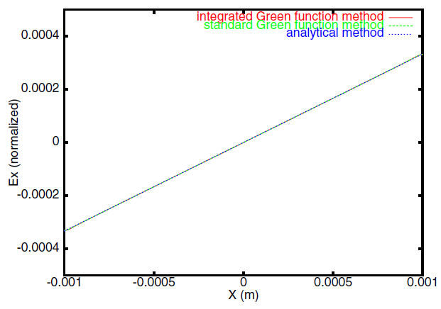
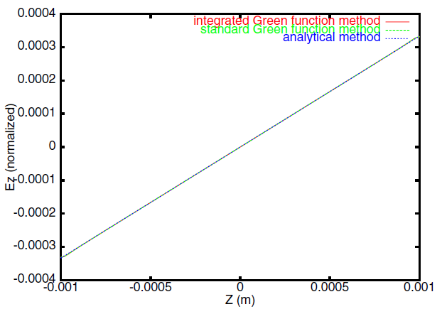
Figure 4: Electric fields along x-axis (left) and along z-axis (right) of a beam with aspect ratio one from solutions of the integrated Green function method, the standard Green function method, and the analytical method.

For a Gaussian beam with an aspect ratio of $30$, the major discrepancy of the electric field occurs around the core, which is given in Fig. 5.

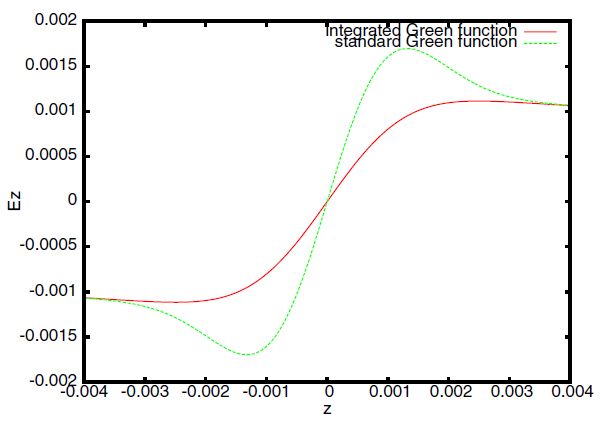
Figure 5: Electric fields along z-axis of a Gaussian beam with aspect ratio $30$ from solutions of the integrated Green function method and the standard Green function method.

These errors in the calculation of electric field for a large aspect ratio beam using the standard Green function method could significantly affect the accuracy of the beam dynamics simulation inside the accelerator.

2.2.2 Multigrid finite difference method for finite boundary condition

In the application, when the effects from the boundary wall become important, other efficient numerical methods should be used to solve the Poisson equation. For a simple regular boundary shape such as rectangular or round shape, efficient Poisson solvers based on the spectral method have been developed [22, 23, 24]. For a complex boundary geometry, the cut-cell multigrid finite difference method can be used to handle the boundary condition [25]. In this method, the differential operator in the Poisson equation is approximated by the difference operator whose numerical accuracy depending on the separation of grid points. Away from the boundary, the separation of grid points is normally uniform, i.e. uniform grid. Near the boundary, nonuniform grid separations are used to fit the geometry of the boundary. By replacing the differential operator with the difference operator, the original Poisson equation is reduced to a group of linear algebraic equations.

For a one-dimensional Poisson equation:

$$\frac{\partial^{2}\phi}{\partial x^{2}} = -\rho/\epsilon_{0}$$ (29)

Using a second-order finite difference approximation on a grid:

$$\frac{\partial^{2}\phi}{\partial x^{2}} \approx \frac{1}{h^{2}}(\phi_{j+1}-2\phi_{j}+\phi_{j-1})$$ (30)

the Poisson equation is reduced to:

$$\frac{1}{h^{2}}(\phi_{j+1}-2\phi_{j}+\phi_{j-1}) = -\rho_{j}/\epsilon_{0}$$ (31)

where $j=1,\cdots,N$, and $N$ is total number of grid points. The above linear algebraic equations can be rewritten in the matrix form:

$$AX = B$$ (32)

where $A$ is a sparse matrix, $X$ denotes the unknown electric potential $\phi$ on grid points, and $B$ denotes the right hand side of the linear algebraic equations. The direct solution of the above matrix equation using the Gaussian elimination will take $O(N^{3})$ operations, which is very inefficient. For a sparse matrix $A$, the above equation is normally solved using an iterative method whose computational cost scales as $O(mN)$. Here $m$ is the number of iterations. Using the iterative method, the above linear algebraic equation can be rewritten as a recursive equation:

$$X^{i+1} = X^{i}+S(B-AX^{i})$$ (33)

where $i=1,\ldots,m$ and $S$ is an approximation to $A^{-1}$ that can be computed quickly, where $S=D^{-1}$ for the Jacobi method, $S=(D+L)^{-1}$ for the Gauss-Seidel method, and $S=\omega(D+\omega L)^{-1}$ for the successive over relaxation (SOR) method, in classical in classical iterative methods. For a fast solver, the number of iterations $m$ has to be reasonably small, i.e. the iteration has to converge to the solution within a small number of iterations. However, for those classical iterative methods, the convergence is slow. These is because those classical iterative methods move information across one grid at a time. It takes about $N^{1/2}$ steps to move information across the grid. After a few iterations, the high frequency errors are smoothed out while the low frequency errors decrease slowly.

The multigrid method is an iterative method based on the concept of smoothing out numerical iteration errors on multiple resolution scales. Instead of solving the original discrete Poisson equation on one fixed mesh size, the multigrid method solves the discrete Poisson problem on multiple levels of mesh size. Fig. 6 shows an example of three level discretization of a 2D computational domain.

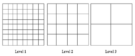
Figure 6: Three-level discretization of a 2D computational domain.

As the discretization level increases, the mesh size increases and the number of unknowns inside the computational domain decreases exponentially. At level three, only one unknown is left for the Dirichlet boundary conditions, which can be solved directly.

The multigrid algorithm using two grid levels consists of five basic operations: pre-smoothing, restriction, evaluation, prolongation, and post-smoothing. During the pre-smoothing stage, an approximate solution of $X^{(i)}$, $\tilde{X}^{(i)}$, is obtained using a classical iterative method such as the Gauss-Seidel iteration:

$$\tilde{X}^{(i)} = (D^{(i)}+L^{(i)})^{-1}U^{(i)}\tilde{X}^{(i)}+(D^{(i)}+L^{(i)})^{-1}B^{(i)}$$ (34)

where $A^{(i)}$ is the discrete Poisson operator at level $i$, $X^{(i)}$ denotes the unknown solution vector at the finest level or the unknown correction vector at other levels, and $B^{(i)}$ is the source vector at the finest level or the residual vector at other levels, $D^{(i)}$, $L^{(i)}$ and $U^{(i)}$ correspond to the main diagonal part, below diagonal part and above diagonal part of the matrix $A^{(i)}$. The residual vector $r^{(i)}$ at this level is calculated from the approximate solution as

$$r^{(i)}=B^{(i)}-A^{(i)}\tilde{X}^{(i)}$$ (35)

These residuals are interpolated from the fine grid $i$ to the coarse grid $i+1$ using a restriction operator $\mathcal{R}$ to obtain the right hand side of the Eq. 32:

$$B^{(i+1)}=\mathcal{R}r^{(i)}$$ (36)

Here, a linear restriction operator $\mathcal{R}$ on a 2D grid is defined as:

$$\mathcal{R} = \left(\begin{array}[]{ccc}\frac{1}{16}&\frac{1}{8}&\frac{1}{16}\\ \frac{1}{8}&\frac{1}{4}&\frac{1}{8}\\ \frac{1}{16}&\frac{1}{8}&\frac{1}{16}\end{array}\right)$$ (40)

which corresponds to a bilinear nine-point interpolation scheme. The evaluation operation on coarse grid $i+1$ will solve the discrete Poisson equation for the correction vector through a direct or an iterative method. The obtained correction is reinterpolated back to the fine grid $i$ from the coarse grid $i+1$ using a prolongation operator. The improved solution on grid level $i$ is given by

$$\tilde{X}^{(i)}_{new}=\tilde{X}^{(i)}+\mathcal{P}\tilde{X}^{(i+1)}$$ (41)

where $\mathcal{P}$ is the prolongation operator:

$$\mathcal{P} = \left(\begin{array}[]{ccc}\frac{1}{4}&\frac{1}{2}&\frac{1}{4}\\ \frac{1}{2}&1&\frac{1}{2}\\ \frac{1}{4}&\frac{1}{2}&\frac{1}{4}\end{array}\right)$$ (45)

which also corresponds to a bilinear interpolation scheme giving nonzero values at nine grid points. This new approximate solution is then used in the classical iterative method as a post-smoothing stage to further improve the accuracy of the solution. If the discrete equation on the coarse grid $i+1$ can be solved using an evaluation operation, only two grid levels are used, and the algorithm is referred to as two-grid method. If the solution on the coarse grid $i+1$ can not be easily attained, the evaluation step can be replaced by more two-grid iterations. Depending on how many two-grid iterations are used when each time the number of grid levels is increased by one, the multigrid iteration can have a V cycle (one two-grid iteration is used) or a W cycle (two two-grid iterations are used) structure [26]. Fig. 7 gives a schematic plot of a V cycle and a W cycle structure with four grid levels.

Figure 7: A schematic plot of a V cycle and a W cycle iteration structure in the multigrid algorithm using four grid levels [26].

Here, $S$ denotes a smoothing operation, $E$ denotes an evaluation operation, each descending line $\backslash$ denotes a restriction operation, and each ascending line $/$ denotes a prolongation operation.

In the multigrid method, the iteration can start from the finest grid level or start from the coarsest grid level. If a good initial guess of the solution is available, starting from the finest grid will be an appropriate method. Otherwise, starting from the coarsest grid will be more efficient since the solution on the coarsest grid can be obtained from the direct evaluation and interpolated to the next finer grid level. The interpolated solution on the finer grid level is used to start the smoothing operation at that level. After some V or W cycle of iterations, the solution at that level is further interpolated to next even finer grid level to start a new smoothing operation and iteration cycle. Such a process is repeated for a number of times until the finest grid level is reached. This type of multigrid iteration is called full multigrid method or nested iteration.

The multigrid method uses more grid levels than the conventional single grid iteration methods. This seems to be more computationally expensive than the single grid iteration. However, by changing the resolution of the discretization, i. e. scale of resolution, from one level to the next level, the low frequency errors in the numerical residues of the iteration can be removed by a coarse grid iteration, while the high frequency errors can be removed on a fine grid iteration. Therefore, the multigrid method uses much less number of iterations on the finest grid level to obtain the converged solution than the single grid iteration method. Most computational work is done on coarse grids with much less number of operations at each grid level compared with the finest grid level iteration. It has been shown that the computational cost of this method scales linearly with the number of grid points [27]. Hence, the multigrid iteration provides a much faster convergence than the classical iterative methods such as the SOR method.

2.3 Numerical integrators for particle advance

With the self-consistent space-charge fields obtained from the solution of the Poisson equation and the external fields, one can advance the particle using a numerical integrator. This involves solving the Lorentz force equations numerically. The Lorentz equations of motion for a charged particle subject to electric and magnetic fields can be written as:

$$\frac{d{\bf r}}{dt} = \frac{{\bf p}c}{\gamma}$$ (46)

$$\frac{d{\bf p}}{dt} = q(\frac{{\bf E}}{mc}+\frac{1}{m\gamma}{\bf p}\times{\bf B})$$ (47)

where ${\bf r}=(x,y,z)$ denotes the particle spatial coordinates, ${\bf p}=(p_{x}/mc,p_{y}/mc,p_{z}/mc)$ the particle normalized mechanic momentum, $m$ the particle rest mass, $q$ the particle charge, $c$ the speed of light in vacuum, $\gamma$ the relativistic factor defined by $\sqrt{1+{\bf p}\cdot{\bf p}}$, $t$ the time, ${\bf E}(x,y,z,t)$ the electric field, and ${\bf B}(x,y,z,t)$ the magnetic field.

For a single step $\tau$, a second-order numerical integrator for the above equation is given by:

$$\zeta(\tau) = {\mathcal{M}}(\tau)\zeta(0)$$ (48)

$$= {\mathcal{M}}_{1}(\tau/2){\mathcal{M}}_{2}(\tau){\mathcal{M}}_{1}(\tau/2)\zeta(0)+O(\tau^{3})$$

The transfer map ${\mathcal{M}}_{1}(\tau/2)$ can be written as:

$$t(\tau/2) = t(0)+\frac{\tau}{2}$$ (49)

$${\bf r}(\tau/2) = {\bf r}(0)+\frac{\tau\bf p}{2\gamma}$$ (50)

The ${\mathcal{M}}_{2}(\tau)$ can have different second-order solutions depending on different ways of approximation. In the Boris algorithm [28], ${\mathcal{M}}_{2}(\tau)$ is given as:

$${\bf p}_{-} = {\bf p}(0)+\frac{q{\bf E}\tau}{2mc}$$ (51)

$$\gamma_{-} = \sqrt{1+{\bf p}_{-}\cdot{\bf p}_{-}}$$ (52)

$${\bf p}_{+}-{\bf p}_{-} = ({\bf p}_{+}+{\bf p}_{-})\times\frac{q{\bf B}\tau}{2m\gamma_{-}}$$ (53)

$${\bf p}(\tau) = {\bf p}_{+}+\frac{q{\bf E}\tau}{2mc}$$ (54)

where ${\bf p}_{+}$ can be solved analytically from the linear equation Eq. 53. The Boris algorithm is time-reversible and has been widely used in numerical plasma simulations [20]. The particle momenta are updated using electric force in Eq. 51 and Eq. 54, and using magnetic force in Eq. 53. The lack of direct cancellation between the electric fields and the magnetic fields can introduce large error to simulate relativistic charged particles dynamics including space-charge effects, where the electric field and the magnetic field cancel each other significantly in the laboratory frame and results in $1/\gamma^{2}$ decrease of the transverse space-charge forces.

Another time-reversible solution for ${\mathcal{M}}_{2}(\tau)$ proposed in reference [29] is given as:

$$\gamma_{0} = \sqrt{1+{\bf p}\cdot{\bf p}}$$ (55)

$${\bf p}_{-} = {\bf p}(0)+\frac{q\tau}{2mc}({\bf E}+c{\bf p}/\gamma_{0}\times{\bf B})$$ (56)

$${\bf p}_{+} = {\bf p}_{-}+\frac{q{\bf E}\tau}{2mc}$$ (57)

$$\gamma_{1} = \sqrt{1+{\bf p}_{+}\cdot{\bf p}_{+}}$$ (58)

$${\bf t} = \frac{q{\bf B}\tau}{2m}$$ (59)

$$\lambda = {\bf p}_{+}\cdot{\bf t}$$ (60)

$$\sigma = \gamma_{1}^{2}-{\bf t}\cdot{\bf t}$$ (61)

$$\gamma_{2} = \sqrt{\frac{\sigma+\sqrt{\sigma^{2}+4({\bf t}\cdot{\bf t}+\lambda^{2})}}{2}}$$ (62)

$${\bf t}^{*} = {\bf t}/\gamma_{2}$$ (63)

$$s = 1/(1+{\bf t}^{*}\cdot{\bf t}^{*})$$ (64)

$${\bf p}(\tau) = s[{\bf p}_{+}+({\bf p}_{+}\cdot{\bf t}^{*}){\bf t}^{*}+{\bf p}_{+}\times{\bf t}^{*}]$$ (65)

This algorithm works well for charged particle tracking with large relativistic factor. However, it is also mathematically more complicated than the Boris algorithm and requires more numerical operations than the Boris integrator.

The source of error in the Boris algorithm results from the lacking appropriate cancellation of the electric force and the magnetic force. This can be solved by updating the momenta using both electric force and magnetic force in the same step instead of separate steps. A simple fast second-order integrator for the transfer map ${\mathcal{M}}_{2}(\tau)$ that avoids the problem of the Boris algorithm was proposed recently and is given as follows [30]:

$${\bf p}_{-} = {\bf p}(0)+\frac{q}{mc}({\bf E}+{\bf v}(0)\times{\bf B})\tau$$ (66)

$${\bf v}_{+} = \frac{{\bf v}(0)+\bf{v}_{-}}{2}$$ (67)

$${\bf p}(\tau) = {\bf p}(0)+\frac{q}{mc}({\bf E}+{\bf v}_{+}\times{\bf B})\tau$$ (68)

where ${\bf v}={\bf p}c/\gamma$. This algorithm includes the direct cancellation of the electric force and the magnetic force from the space-charge fields and works well for large relativistic factor. It also has a simpler mathematical form and requires less numerical operations than the Boris integrator and the integrator in Eqs. 55-65. This algorithm converges to the solution of the above integrator if one repeats Eqs. 66-68 many times. However, this is not necessary since the iteration does not increase the order of accuracy of the algorithm. It is shown in the following examples that the new numerical integrator agrees with the integrator in Eqs. 55-65 very well.

2.3.1 Benchmark of the numerical integrators

The above second-order numerical integrator were benchmarked using the following numerical example. In this example, we considered an electron moving inside the static electric and magnetic fields generated by a co-moving positron beam. These fields are given as:

$$E_{x} = E_{0}x\gamma_{0}$$ (69)

$$E_{y} = E_{0}y\gamma_{0}$$ (70)

$$E_{z} = 0$$ (71)

$$B_{x} = -E_{0}y\gamma_{0}\beta_{0}/c$$ (72)

$$B_{y} = E_{0}x\gamma_{0}\beta_{0}/c$$ (73)

$$B_{z} = 0$$ (74)

where $\gamma_{0}$ is the relativistic factor of the moving positron beam, $\beta_{0}=\sqrt{1-(1/\gamma_{0})^{2}}$, and the constant $E_{0}=9\times 10^{6}V/m^{2}$. The above fields correspond to the space-space fields generated by the co-moving infinitely long transversely uniform cylindrical positron beam.

We assumed that both the initial electron and the co-moving positron beam have a kinetic energy of $100$ MeV. Fig. 8 shows the electron $x$ coordinate evolution as a function of time from the Boris integrator (magenta), the integrator proposed by Vay (green), the new integrator (blue) with a step size of $1$ ns (around $0.001$ oscillation period), and the analytical solution (red). Here, the analytical solution is obtained in the co-moving frame without including the relativistic effects and then Lorentz transformed back to the laboratory frame. The analytical solution for the $x$ trajectory starting with initial $0$ momentum is given as:

$$x(t) = x_{0}\cos(\sqrt{qE_{0}/m}/\gamma_{0}t)$$ (75)

where $x_{0}=1$ mm is the initial horizontal position.

Figure 8: Particle $x$ coordinate evolution as a function of time from the Boris integrator (magenta), the Vay integrator (green), the new integrator (blue), and the analytical solution (red) for an electron with $100$ MeV kinetic energy.

It is seen that after one oscillation period, the solution from the Boris integrator starts to deviate from the other solutions while the other three solutions are still on top of each other. Fig. 9 shows the relative numerical errors at the end of the above integration as a function of time step size from the Boris integrator, the Vay integrator, and the new integrator.

Figure 9: Relative numerical errors at the end of the above integration as a function of step size from the Boris integrator (magenta), the Vay integrator (green), and the new integrator (blue) for an electron with $100$ MeV kinetic energy. A quadratic monomial function is also plotted here (red).

As expected, all three second-order accuracy numerical integrators converge quadratically with respect to the time step size. However, the errors from the Boris integrator are about $4$ orders of magnitude larger than those from the other two integrators.

In the second example, we tracked a $100$ MeV electron in the above electric and magnetic fields for more $500,000$ periods using the new second-order numerical integrator with time step size of $100$ ns. The relative kinetic energy growth as a function of time is shown in Fig. 10. It is seen that except the oscillation from energy exchange, there is no steady state secular energy increase or decrease resulting from numerical heating or damping of the proposed new integrator.

Figure 10: Relative kinetic energy growth evolution of an initial $100$ MeV electron.

Fig. 11 shows the phase space trajectory of the electron from the proposed new algorithm and from the Vay algorithm. It is seen that both integrators agree with each other very well. The phase space structure is well preserved after $500,000$ periods.

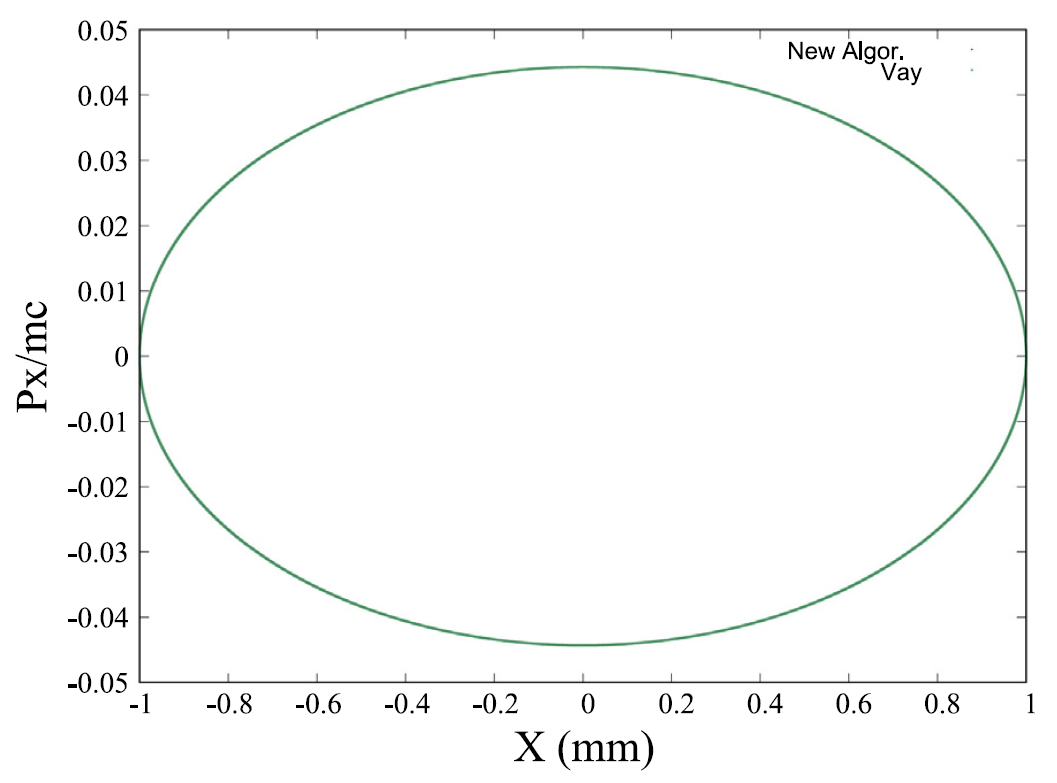
Figure 11: Electron phase space trajectory from the new integrator and the Vay integrator.

3 Symplectic self-consistent space-charge tracking models

The above grid based, momentum conserved, particle-in-cell method does not satisfy the symplectic condition of classic multi-particle dynamics. Violating the symplectic condition in multi-particle tracking might not be an issue in a single pass system such as a linear accelerator. But in a circular accelerator, violating the symplectic condition may result in undesired numerical errors in the long-term tracking simulation. Recently, symplectic multi-particle model was proposed for self-consistent space-charge simulations [31, 32].

In the accelerator beam dynamics simulation, for a multi-particle system with $N_{p}$ charged particles subject to both a space-charge self field and an external field, an approximate Hamiltonian of the system can be written as [33]:

$$H = \sum_{i=1}^{N_{p}}{\bf p}_{i}^{2}/2+\frac{1}{2}\sum_{i=1}^{N_{p}}\sum_{j=1}^{N_{p}}q\bar{\varphi}({\bf r}_{i},{\bf r}_{j})+\sum_{i=1}^{N_{p}}q\psi({\bf r}_{i})$$ (76)

where $H({\bf r}_{1},{\bf r}_{2},\cdots,{\bf r}_{N_{p}},{\bf p}_{1},{\bf p}_{2},\cdots,{\bf p}_{N_{p}};s)$ denotes the Hamiltonian of the system using distance $s$ as an independent variable, $\bar{\varphi}$ is the space-charge interaction potential (including both the direct electric potential and the longitudinal vector potential) between the charged particles $i$ and $j$ (subject to appropriate boundary conditions), $\psi$ denotes the potential associated with the external field, ${\bf r}_{i}=(x_{i},y_{i},\theta_{i}=\omega\Delta t)$ denotes the normalized canonical spatial coordinates of particle $i$, ${\bf p}_{i}=(p_{xi},p_{yi},p_{ti}=-\Delta E/mc^{2})$ the normalized canonical momentum coordinates of particle $i$, and $\omega$ the reference angular frequency, $\Delta t$ the time of flight to location $s$, $\Delta E$ the energy deviation with respect to the reference particle, $m$ the rest mass of the particle, and $c$ the speed of light in vacuum. The equations governing the motion of individual particle $i$ follow the Hamilton’s equations as:

$$\frac{d{\bf r}_{i}}{ds} = \frac{\partial H}{\partial{\bf p}_{i}}$$ (77)

$$\frac{d{\bf p}_{i}}{ds} = -\frac{\partial H}{\partial{\bf r}_{i}}$$ (78)

Let $\zeta$ denote a 6N-vector of coordinates, the above Hamilton’s equation can be rewritten as:

$$\frac{d\zeta}{ds} = -[H,\zeta]$$ (79)

where [ , ] is the Poisson bracket. A formal solution for the above equation after a single step $\tau$ can be written as:

$$\zeta(\tau) = \exp(-\tau(:H:))\zeta(0)$$ (80)

Here, we have defined a differential operator $:H:$ as $:H:g=[H,\ g]$, for arbitrary function $g$. For a Hamiltonian that can be written as a sum of two terms $H=H_{1}+H_{2}$, an approximate solution to above formal solution can be written as [34]

$$\zeta(\tau) = \exp(-\tau(:H_{1}:+:H_{2}:))\zeta(0)$$ (81)

$$= \exp(-\frac{1}{2}\tau:H_{1}:)\exp(-\tau:H_{2}:)\exp(-\frac{1}{2}\tau:H_{1}:)\zeta(0)+O(\tau^{3})$$

Let $\exp(-\frac{1}{2}\tau:H_{1}:)$ define a transfer map ${\mathcal{M}}_{1}$ and $\exp(-\tau:H_{2}:)$ a transfer map ${\mathcal{M}}_{2}$, for a single step, the above splitting results in a second order numerical integrator for the original Hamilton’s equation as:

$$\zeta(\tau) = {\mathcal{M}}(\tau)\zeta(0)$$ (82)

$$= {\mathcal{M}}_{1}(\tau/2){\mathcal{M}}_{2}(\tau){\mathcal{M}}_{1}(\tau/2)\zeta(0)+O(\tau^{3})$$

The above numerical integrator can be extended to $4^{th}$ order accuracy and arbitrary even-order accuracy following Yoshida’s approach [35]. This numerical integrator Eq. 82 will be symplectic if both the transfer map ${\mathcal{M}}_{1}$ and the transfer map ${\mathcal{M}}_{2}$ are symplectic. A transfer map ${\mathcal{M}}_{i}$ is symplectic if and only if the Jacobian matrix $M_{i}$ of the transfer map ${\mathcal{M}}_{i}$ satisfies the following condition:

$$M_{i}^{T}JM_{i}=J$$ (83)

where $J$ denotes the $6N\times 6N$ matrix given by:

$$J=\left(\begin{array}[]{cc}0&I\\ -I&0\end{array}\right)$$ (84)

and $I$ is the $3N\times 3N$ identity matrix.

For the Hamiltonian in Eq. 76, we can choose $H_{1}$ as:

$$H_{1} = \sum_{i=1}^{N_{p}}{\bf p}_{i}^{2}/2+\sum_{i=1}^{N_{p}}q\psi({\bf r}_{i})$$ (85)

This corresponds to the Hamiltonian of a group of charged particles inside an external field without mutual interaction among themselves. The charged particle magnetic optics method can be used to find the symplectic transfer map ${\mathcal{M}}_{1}$ for this Hamiltonian with the external fields from most accelerator beam line elements [33, 36, 37].

We can choose $H_{2}$ as:

$$H_{2} = \frac{1}{2}\sum_{i=1}^{N_{p}}\sum_{j=1}^{N_{p}}q{\bar{\varphi}}({\bf r}_{i},{\bf r}_{j})$$ (86)

which includes the space-charge effect and is only a function of position. For the space-charge Hamiltonian $H_{2}({\bf r})$, the single step transfer map ${\mathcal{M}}_{2}$ can be written as:

$${\bf r}_{i}(\tau) = {\bf r}_{i}(0)$$ (87)

$${\bf p}_{i}(\tau) = {\bf p}_{i}(0)-\frac{\partial H_{2}({\bf r})}{\partial{\bf r}_{i}}\tau$$ (88)

The Jacobi matrix of the above transfer map ${\mathcal{M}}_{2}$ is

$$M_{2}=\left(\begin{array}[]{cc}I&0\\ L&I\end{array}\right)$$ (89)

where $L$ is a $3N\times 3N$ matrix. For $M_{2}$ to satisfy the symplectic condition Eq. 83, the matrix $L$ needs to be a symmetric matrix, i.e.

$$L=L^{T}$$ (90)

Given the fact that $L_{ij}=\partial{\bf p}_{i}(\tau)/\partial{\bf r}_{j}=-\frac{\partial^{2}H_{2}({\bf r})}{\partial{\bf r}_{i}\partial{\bf r}_{j}}\tau$, the matrix $L$ will be symmetric as long as it is analytically calculated from the function $H_{2}$. If both the transfer map ${\mathcal{M}}_{1}$ and the transfer map ${\mathcal{M}}_{2}$ are symplectic, the numerical integrator Eq. 48 for multi-particle tracking will be symplectic.

For a coasting beam, the Hamiltonian $H_{2}$ can be written as [33]:

$$H_{2} = \frac{K}{2}\sum_{i=1}^{N_{p}}\sum_{j=1}^{N_{p}}\varphi({\bf r}_{i},{\bf r}_{j})$$ (91)

where $K=qI/(2\pi\epsilon_{0}p_{0}v_{0}^{2}\gamma_{0}^{2})$ is the generalized perveance, $I$ is the beam current, $\epsilon_{0}$ is the permittivity of vacuum, $p_{0}$ is the momentum of the reference particle, $v_{0}$ is the speed of the reference particle, $\gamma_{0}$ is the relativistic factor of the reference particle, and $\varphi$ is the space charge Coulomb interaction potential. In this Hamiltonian, the effects of the direct Coulomb electric potential and the longitudinal vector potential are combined together. The electric Coulomb potential $\varphi$ in the Hamiltonian $H_{2}$ can be obtained from the solution of the Poisson equation. In the following, we assume that the coasting beam is inside a rectangular perfectly conducting pipe. In this case, the two-dimensional Poisson’s equation can be written as:

$$\frac{\partial^{2}\phi}{\partial x^{2}}+\frac{\partial^{2}\phi}{\partial y^{2}}=-4\pi\rho$$ (92)

where $\phi$ is the electric potential, and $\rho$ is the particle density distribution of the beam.

The boundary conditions for the electric potential inside the rectangular perfectly conducting pipe are:

$$\phi(x=0,y) = 0$$ (93)

$$\phi(x=a,y) = 0$$ (94)

$$\phi(x,y=0) = 0$$ (95)

$$\phi(x,y=b) = 0$$ (96)

where $a$ is the horizontal width of the pipe and $b$ is the vertical width of the pipe.

Given the boundary conditions in Eqs. 93-96, the electric potential $\phi$ and the source term $\rho$ can be approximated using two sine functions as [22, 24, 38, 39, 40]:

$$\rho(x,y)=\sum_{l=1}^{N_{l}}\sum_{m=1}^{N_{m}}\rho^{lm}\sin(\alpha_{l}x)\sin(\beta_{m}y)$$ (97)

$$\phi(x,y)=\sum_{l=1}^{N_{l}}\sum_{m=1}^{N_{m}}\phi^{lm}\sin(\alpha_{l}x)\sin(\beta_{m}y)$$ (98)

where

$$\rho^{lm}=\frac{4}{ab}\int_{0}^{a}\int_{0}^{b}\rho(x,y)\sin(\alpha_{l}x)\sin(\beta_{m}y)\ dxdy$$ (99)

$$\phi^{lm}=\frac{4}{ab}\int_{0}^{a}\int_{0}^{b}\phi(x,y)\sin(\alpha_{l}x)\sin(\beta_{m}y)\ dxdy$$ (100)

where $\alpha_{l}=l\pi/a$ and $\beta_{m}=m\pi/b$. The above approximation follows the numerical spectral Galerkin method since each basis functions satisfies the boundary conditions on the wall [38, 40, 39]. For a smooth function, this spectral approximation has an accuracy whose numerical error scales as $O(\exp(-cN))$ with $c>0$, where $N$ is the number of the basis function (i.e. mode number in each dimension) used in the approximation. By substituting above expansions into the Poisson Eq. 92 and making use of the orthonormal condition of the sine functions, we obtain

$$\phi^{lm} = \frac{4\pi\rho^{lm}}{\gamma_{lm}^{2}}$$ (101)

where $\gamma_{lm}^{2}=\alpha_{l}^{2}+\beta_{m}^{2}$.

In the simulation, the particle density distribution function $\rho(x,y)$ can be represented as:

$$\rho(x,y) = \frac{1}{\Delta x\Delta yN_{p}}\sum_{j=1}^{N_{p}}S(x-x_{j})S(y-y_{j})$$ (102)

where $S(x)$ is the unitless shape function (i.e. deposition function in the PIC model) $\Delta x$ and $\Delta y$ are mesh size in each dimension. The use of the shape function helps smooth the density function when the number of macroparticles in the simulation is much less than the real number of particles in the beam. Using the above equation and Eq. 99 and Eq. 101, we obtain:

$$\phi^{lm} = \frac{4\pi}{\gamma_{lm}^{2}}\frac{4}{ab}\frac{1}{N_{p}}\sum_{j=1}^{N_{p}}\frac{1}{\Delta x\Delta y}\int_{0}^{a}\int_{0}^{b}S(x-x_{j})S(y-y_{j})\sin(\alpha_{l}x)\sin(\beta_{m}y)dxdy$$ (103)

and the electric potential as:

$$\phi(x,y)={4\pi}\frac{4}{ab}\frac{1}{N_{p}}\sum_{j=1}^{N_{p}}\sum_{l=1}^{N_{l}}\sum_{m=1}^{N_{m}}\frac{1}{\gamma_{lm}^{2}}\sin(\alpha_{l}x)\sin(\beta_{m}y)$$

$$\frac{1}{\Delta x\Delta y}\int_{0}^{a}\int_{0}^{b}S(\bar{x}-x_{j})S(\bar{y}-y_{j})\sin(\alpha_{l}\bar{x})\sin(\beta_{m}\bar{y})d\bar{x}d\bar{y}$$ (104)

The electric potential at a particle $i$ location can be obtained from the potential as:

$$\phi(x_{i},y_{i}) = \frac{1}{\Delta x\Delta y}\int_{0}^{a}\int_{0}^{b}\phi(x,y)S(x-x_{i})S(y-y_{i})dxdy$$ (105)

$$= {4\pi}\frac{4}{ab}\frac{1}{N_{p}}\sum_{j=1}^{N_{p}}\sum_{l=1}^{N_{l}}\sum_{m=1}^{N_{m}}\frac{1}{\gamma_{lm}^{2}}\frac{1}{\Delta x\Delta y}\int_{0}^{a}\int_{0}^{b}S(x-x_{i})S(y-y_{i})\sin(\alpha_{l}x)\sin(\beta_{m}y)dxdy$$

$$\frac{1}{\Delta x\Delta y}\int_{0}^{a}\int_{0}^{b}S(x-x_{j})S(y-y_{j})\sin(\alpha_{l}x)\sin(\beta_{m}y)dxdy$$

where the interpolation function to the particle location is assumed to be the same as the deposition function.

From the above electric potential, the interaction potential $\varphi$ between particles $i$ and $j$ can be written as:

$$\varphi(x_{i},y_{i},x_{j},y_{j}) = {4\pi}\frac{4}{ab}\frac{1}{N_{p}}\sum_{l=1}^{N_{l}}\sum_{m=1}^{N_{m}}\frac{1}{\gamma_{lm}^{2}}\frac{1}{\Delta x\Delta y}\int_{0}^{a}\int_{0}^{b}S(x-x_{j})S(y-y_{j})\sin(\alpha_{l}x)\sin(\beta_{m}y)dxdy$$ (106)

$$\frac{1}{\Delta x\Delta y}\int_{0}^{a}\int_{0}^{b}S(x-x_{i})S(y-y_{i})\sin(\alpha_{l}x)\sin(\beta_{m}y)dxdy$$

Now, the space-charge Hamiltonian $H_{2}$ can be written as:

$$H_{2} = 4\pi\frac{K}{2}\frac{4}{ab}\frac{1}{N_{p}}\sum_{i=1}^{N_{p}}\sum_{j=1}^{N_{p}}\sum_{l=1}^{N_{l}}\sum_{m=1}^{N_{m}}\frac{1}{\gamma_{lm}^{2}}$$ (107)

$$\frac{1}{\Delta x\Delta y}\int_{0}^{a}\int_{0}^{b}S(x-x_{j})S(y-y_{j})\sin(\alpha_{l}x)\sin(\beta_{m}y)dxdy$$

$$\frac{1}{\Delta x\Delta y}\int_{0}^{a}\int_{0}^{b}S(x-x_{i})S(y-y_{i})\sin(\alpha_{l}x)\sin(\beta_{m}y)dxdy$$

3.1 Symplectic gridless particle model

In the symplectic gridless particle space-charge model, the shape function is assumed to be a Dirac delta function and the particle distribution function $\rho(x,y)$ can be represented as:

$$\rho(x,y)=\frac{1}{N_{p}}\sum_{j=1}^{N_{p}}\delta(x-x_{j})\delta(y-y_{j})$$ (108)

Now, the space-charge Hamiltonian $H_{2}$ can be written as:

$$H_{2}=4\pi\frac{K}{2}\frac{4}{ab}\frac{1}{N_{p}}\sum_{i=1}^{N_{p}}\sum_{j=1}^{N_{p}}\sum_{l=1}^{N_{l}}\sum_{m=1}^{N_{m}}\frac{1}{\gamma_{lm}^{2}}\sin(\alpha_{l}x_{j})\sin(\beta_{m}y_{j})\sin(\alpha_{l}x_{i})\sin(\beta_{m}y_{i})$$ (109)

The one-step symplectic transfer map ${\mathcal{M}}_{2}$ of the particle $i$ with this Hamiltonian is given as:

$$p_{xi}(\tau) = p_{xi}(0)-\tau 4\pi{K}\frac{4}{ab}\frac{1}{N_{p}}\sum_{j=1}^{N_{p}}\sum_{l=1}^{N_{l}}\sum_{m=1}^{N_{m}}\frac{\alpha_{l}}{\gamma_{lm}^{2}}\sin(\alpha_{l}x_{j})\sin(\beta_{m}y_{j})\cos(\alpha_{l}x_{i})\sin(\beta_{m}y_{i})$$

$$p_{yi}(\tau) = p_{yi}(0)-\tau 4\pi{K}\frac{4}{ab}\frac{1}{N_{p}}\sum_{j=1}^{N_{p}}\sum_{l=1}^{N_{l}}\sum_{m=1}^{N_{m}}\frac{\beta_{m}}{\gamma_{lm}^{2}}\sin(\alpha_{l}x_{j})\sin(\beta_{m}y_{j})\sin(\alpha_{l}x_{i})\cos(\beta_{m}y_{i})$$ (110)

Here, both $p_{xi}$ and $p_{yi}$ are normalized by the reference particle momentum $p_{0}$.

3.2 Symplectic particle-in-cell model

If the deposition/interpolation shape function is not a delta function, the one-step symplectic transfer map ${\mathcal{M}}_{2}$ of the particle $i$ with this space-charge Hamiltonian $H_{2}$ is given as:

$$p_{xi}(\tau) = p_{xi}(0)-\tau 4\pi{K}\frac{4}{ab}\frac{1}{N_{p}}\sum_{j=1}^{N_{p}}\sum_{l=1}^{N_{l}}\sum_{m=1}^{N_{m}}\frac{1}{\gamma_{lm}^{2}}\frac{1}{\Delta x\Delta y}\int_{0}^{a}\int_{0}^{b}S(x-x_{j})S(y-y_{j})\sin(\alpha_{l}x)\sin(\beta_{m}y)dxdy$$

$$\frac{1}{\Delta x\Delta y}\int_{0}^{a}\int_{0}^{b}\frac{\partial S(x-x_{i})}{\partial x_{i}}S(y-y_{i})\sin(\alpha_{l}x)\sin(\beta_{m}y)dxdy$$

$$p_{yi}(\tau) = p_{yi}(0)-\tau 4\pi{K}\frac{4}{ab}\frac{1}{N_{p}}\sum_{j=1}^{N_{p}}\sum_{l=1}^{N_{l}}\sum_{m=1}^{N_{m}}\frac{1}{\gamma_{lm}^{2}}\frac{1}{\Delta x\Delta y}\int_{0}^{a}\int_{0}^{b}S(x-x_{j})S(y-y_{j})\sin(\alpha_{l}x)\sin(\beta_{m}y)dxdy$$ (111)

$$\frac{1}{\Delta x\Delta y}\int_{0}^{a}\int_{0}^{b}S(x-x_{i})\frac{\partial S(y-y_{i})}{\partial y_{i}}\sin(\alpha_{l}x)\sin(\beta_{m}y)dxdy$$

where both $p_{xi}$ and $p_{yi}$ are normalized by the reference particle momentum $p_{0}$, and $S^{\prime}(x)$ is the first derivative of the shape function. Assuming that the shape function is a compact local function with respect to the computational grid, after approximating the integral with summation on the grid, the above map can be rewritten as:

$$p_{xi}(\tau) = p_{xi}(0)-\tau 4\pi{K}\frac{4}{ab}\frac{1}{N_{p}}\sum_{j=1}^{N_{p}}\sum_{l=1}^{N_{l}}\sum_{m=1}^{N_{m}}\frac{1}{\gamma_{lm}^{2}}\sum_{I^{\prime}}\sum_{J^{\prime}}S(x_{I^{\prime}}-x_{j})S(y_{J^{\prime}}-y_{j})\sin(\alpha_{l}x_{I^{\prime}})\sin(\beta_{m}y_{J^{\prime}})$$

$$\sum_{I}\sum_{J}\frac{\partial S(x_{I}-x_{i})}{\partial x_{i}}S(y_{J}-y_{i})\sin(\alpha_{l}x_{I})\sin(\beta_{m}y_{J})$$

$$p_{yi}(\tau) = p_{yi}(0)-\tau 4\pi{K}\frac{4}{ab}\frac{1}{N_{p}}\sum_{j=1}^{N_{p}}\sum_{l=1}^{N_{l}}\sum_{m=1}^{N_{m}}\frac{1}{\gamma_{lm}^{2}}\sum_{I^{\prime}}\sum_{J^{\prime}}S(x_{I^{\prime}}-x_{j})S(y_{J^{\prime}}-y_{j})\sin(\alpha_{l}x_{I^{\prime}})\sin(\beta_{m}y_{J^{\prime}})$$ (112)

$$\sum_{I}\sum_{J}S(x_{I}-x_{i})\frac{\partial S(y_{I}-y_{i})}{\partial y_{i}}\sin(\alpha_{l}x_{I})\sin(\beta_{m}y_{J})$$

where the integers $I$, $J$, $I^{\prime}$, and $J^{\prime}$ denote the two dimensional computational grid index, and the summations with respect to those indices are limited to the range of a few local grid points depending on the specific deposition function. If one defines the density related function $\bar{\rho}(x_{I^{\prime}},y_{J^{\prime}})$ on the grid as:

$$\bar{\rho}(x_{I^{\prime}},y_{J^{\prime}})=\frac{1}{N_{p}}\sum_{j=1}^{N_{p}}S(x_{I^{\prime}}-x_{j})S(y_{J^{\prime}}-y_{j}),$$ (113)

the above space-charge map can be rewritten as:

$$p_{xi}(\tau) = p_{xi}(0)-\tau 4\pi{K}\sum_{I}\sum_{J}\frac{\partial S(x_{I}-x_{i})}{\partial x_{i}}S(y_{J}-y_{i})[\frac{4}{ab}\sum_{l=1}^{N_{l}}\sum_{m=1}^{N_{m}}\frac{1}{\gamma_{lm}^{2}}$$

$$\sum_{I^{\prime}}\sum_{J^{\prime}}\bar{\rho}(x_{I^{\prime}},y_{J^{\prime}})\sin(\alpha_{l}x_{I^{\prime}})\sin(\beta_{m}y_{J^{\prime}})\sin(\alpha_{l}x_{I})\sin(\beta_{m}y_{J})]$$

$$p_{yi}(\tau) = p_{yi}(0)-\tau 4\pi{K}\sum_{I}\sum_{J}S(x_{I}-x_{i})\frac{\partial S(y_{I}-y_{i})}{\partial y_{i}}[\frac{4}{ab}\sum_{l=1}^{N_{l}}\sum_{m=1}^{N_{m}}\frac{1}{\gamma_{lm}^{2}}$$ (114)

$$\sum_{I^{\prime}}\sum_{J^{\prime}}\bar{\rho}(x_{I^{\prime}},y_{J^{\prime}})\sin(\alpha_{l}x_{I^{\prime}})\sin(\beta_{m}y_{J^{\prime}})\sin(\alpha_{l}x_{I})\sin(\beta_{m}y_{J})]$$

It turns out that the expression inside the bracket corresponds to the solution of potential on grid using the charge density on grid, which can be written as:

$$\phi(x_{I},y_{J}) = \frac{4}{ab}\sum_{l=1}^{N_{l}}\sum_{m=1}^{N_{m}}\frac{1}{\gamma_{lm}^{2}}\sum_{I^{\prime}}\sum_{J^{\prime}}{\bar{\rho}}(x_{I^{\prime}},y_{J^{\prime}})\sin(\alpha_{l}x_{I^{\prime}})\sin(\beta_{m}y_{J^{\prime}})\sin(\alpha_{l}x_{I})\sin(\beta_{m}y_{J})$$ (115)

Then the above space-charge map can be rewritten in a more concise form as:

$$p_{xi}(\tau) = p_{xi}(0)-\tau 4\pi{K}\sum_{I}\sum_{J}\frac{\partial S(x_{I}-x_{i})}{\partial x_{i}}S(y_{J}-y_{i})\phi(x_{I},y_{J})$$

$$p_{yi}(\tau) = p_{yi}(0)-\tau 4\pi{K}\sum_{I}\sum_{J}S(x_{I}-x_{i})\frac{\partial S(y_{J}-y_{i})}{\partial y_{i}}\phi(x_{I},y_{J})$$ (116)

In the PIC literature, a compact function such as a linear function or a quadratic function is used in the simulation. For example, the derivative of the above TSC function can be written as:

$$\frac{\partial S(x_{I}-x_{i})}{\partial x_{i}} = \left\{\begin{array}[]{ll}-2(\frac{x_{i}-x_{I}}{\Delta x})/\Delta x,&|x_{i}-x_{I}|\leq\Delta x/2\\ (-\frac{3}{2}+\frac{(x_{i}-x_{I})}{\Delta x})/\Delta x,&\Delta x/2<|x_{i}-x_{I}|\leq 3/2\Delta x,\ \ x_{i}>x_{I}\\ (\frac{3}{2}+\frac{(x_{i}-x_{I})}{\Delta x})/\Delta x,&\Delta x/2<|x_{i}-x_{I}|\leq 3/2\Delta x,\ \ x_{i}\leq x_{I}\\ 0&{\rm otherwise}\end{array}\right.$$ (121)

The same shape function and its derivative can be applied to the $y$ dimension.

Using the symplectic transfer map ${\mathcal{M}}_{1}$ for the external field Hamiltonian $H_{1}$ from a magnetic optics code and the transfer map ${\mathcal{M}}_{2}$ for space-charge Hamiltonian $H_{2}$, one obtains a symplectic PIC model including the self-consistent space-charge effects.

3.3 Benchmark of multi-particle tracking models

The above self-consistent multi-particle tracking models were benchmarked in an application example. In this example, a one $GeV$ proton beam subject to strong space-charge driven resonance transported through a linear periodic quadrupole focusing and defocusing (FODO) channel inside a rectangular perfectly conducting pipe. It was tracked including self-consistent space-charge effects for several hundred thousands of lattice periods using the symplectic gridless model, the symplectic particle-in-cell model and the nonsymplectic particle-in-cell model. A schematic plot of the lattice is shown in Fig. 12.

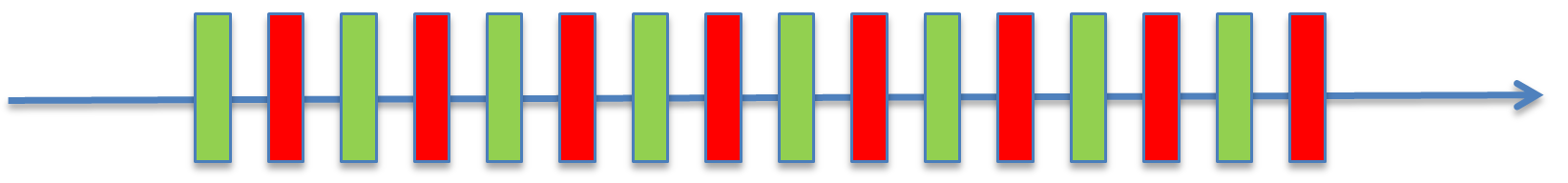
Figure 12: Schematic plot of a FODO lattice.

It consists of a $0.1$ m focusing quadrupole magnet and a $0.1$ m defocusing quadrupole magnet within a single period. The total length of the period is $1$ meter. The zero current phase advance through one lattice period is $85$ degrees. The current of the beam is $450$ A and the depressed phase advance is $42$ degrees. Such a high current drives the beam across the $4^{th}$ order collective instability [41]. The initial transverse normalized emittance of the proton beam is $1$ $\mu m$ with a 4D Gaussian distribution.

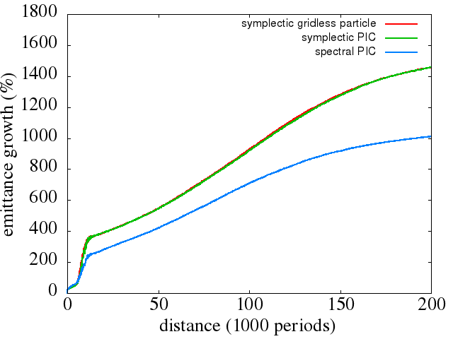
Figure 13: Four dimensional emittance growth evolution from the symplectic gridless particle model (red), the symplectic PIC model (green), and the nonsymplectic spectral PIC (blue).

Fig. 13 shows the four dimensional emittance growth $(\frac{\epsilon_{x}}{\epsilon_{x0}}\frac{\epsilon_{y}}{\epsilon_{y0}}-1)\%$ evolution through $200,000$ lattice periods from the symplectic gridless particle model, from the symplectic PIC model, and from the nonsymplectic spectral PIC model. These simulations used about $50,000$ macroparticles and $15\times 15$ modes in the spectral Poisson solver. In both PIC models, $257\times 257$ grid points are used to obtain the density distribution function on the grid. The perfectly conducting pipe has a square shape with an aperture size of $10$ mm. It is seen that the symplectic PIC model and the symplectic gridless particle model agrees with each other very well. The nonsymplectic spectral PIC model yields significantly smaller emittance growth than those from the two symplectic methods, which might result from the numerical damping effects in the nonsymplectic integrator. The fast emittance growth within the first $20,000$ periods is caused by the space-charge driven $4^{th}$ order collective instability. The slow emittance growth after $20,000$ periods might be due to numerical collisional effects.

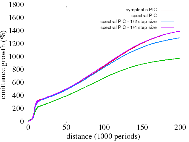
Figure 14: Four dimensional emittance growth evolution from the symplectic PIC model (red), the nonsymplectic spectral PIC with the nominal step size (green), the spectral PIC with half of the nominal step size (blue), and the spectral PIC with one quarter of the nominal step size (pink).

The accuracy of the nonsymplectic PIC model can be improved with finer step size. Fig. 14 shows the 4D emittance growth evolution from the symplectic PIC model and those from the nonsymplectic PIC model with the same nominal step size, from the nonsymplectic PIC model with one-half of the nominal step size, and from the nonsymplectic PIC model with one-quarter of the nominal step size. It is seen that as the step size decreases, the emittance growth from the nonsymplectic PIC model converges towards that from the symplectic PIC model.

The computational complexity of the PIC model is proportional to the $O(N_{grid}log(N_{grid})+N_{p})$, where $N_{grid}$ and $N_{p}$ are total number of computational grid points and macroparticles used in the simulation. The computational complexity of the symplectic gridless particle model is proportional to the $O(N_{mode}N_{p})$, where $N_{mode}$ is the total number of modes for the space-charge solver. On a single processor computer, with a large number of macroparticles used, the symplectic PIC model is computationally more efficient than the symplectic gridless particle model. However, on a massive parallel computer, the scalability of the symplectic PIC model may be limited by the challenges of work load balance among multiple processors and communication associated with the grided based space-charge solver and the particle manager [42]. The symplectic gridless particle model has regular data structure for perfect work load balance and small amount of communication associated with the space-charge solver. It scales well on both multiple processor Central Processing Unit (CPU) computers and multiple Graphic Processing Unit (GPU) computers [43].

References

- [1] R. Ryne and S. Habib, in Computational Accelerator Physics, edited by J. J. Bisognano and A. A. Mondelli, AIP Conference Proceedings 391 (Woodbury, New York, 1997) p. 377.
- [2] B.B.Godfrey,in Computer Applications in Plasma Science and Engineering, edited by A.T.Drobot (Springer Verlag, New York, 1991.)
- [3] A. Friedman, D. P. Grote, and I. Haber, Phys. Fluids B 4, 2203 (1992).
- [4] M. E. Jones, B. E. Carlsten, M. J. Schmitt, C. A. Aldrich, and E. L. Lindman, Nucl. Instrum. Methods Phys. Res. A 318, 323 (1992).
- [5] R. Ryne, ed., Computational Accelerator Physics, AIP Conference Proceedings 297 (Los Alamos, NM, 1993).
- [6] H. Takeda and J. H. Billen, Recent developments of the accelerator design code PARMILA, in Proc. XIX International Linac Conference, Chicago, August 1998, p. 156.
- [7] S. Machida and M. Ikegami, in AIP Conf. Proc 448, p.73 (1998).
- [8] F. W. Jones and H. O. Schoenauer, Proc of PAC1999, p. 2933, 1999.
- [9] J. Qiang, R. D. Ryne, S. Habib, V. Decyk, J. Comput. Phys. 163, 434, 2000.
- [10] P. N. Ostroumov and K. W. Shepard. Phys. Rev. ST. Accel. Beams 11, 030101 (2001).
- [11] R. Duperrier, Phys. Rev. ST Accel. Beams 3, 124201, 2000.
- [12] J. D. Galambos, S. Danilov, D. Jeon, J. A. Holmes, and D. K. Olsen, F. Neri and M. Plum, Phys. Rev. ST Accel. Beams 3, 034201, (2000).
- [13] H. Qin, R. C. Davidson, W. W. Lee, and R. Kolesnikov, Nucl. Instr. Meth. in Phys. Res. A 464, 477 (2001).
- [14] J. Qiang, S. Lidia, R. D. Ryne, and C. Limborg-Deprey, Phys. Rev. ST Accel. Beams 9, 044204, 2006.
- [15] J. Amundson, P. Spentzouris, J. Qiang and R. Ryne, J. Comp. Phys. vol. 211, 229 (2006).
- [16] http://amas.web.psi.ch/docs/opal/opal_user_guide.pdf.
- [17] J. Qiang, R. D. Ryne, M. Venturini, A. A. Zholents, and I. V. Pogorelov, Phys. Rev. ST Accel. Beams 12, 100702, 2009.
- [18] https://en.wikipedia.org/wiki/Leapfrog_integration
- [19] R.W. Hockney, J.W. Eastwood, Computer Simulation Using Particles,Adam Hilger, New York, 1988.
- [20] C. K. Birdsall and A. B. Langdon, Plasma Physics via Computer Simulation,(CRC Press, New York, 2004), p. 174.
- [21] J. Qiang, S. Lidia, R. D. Ryne, and C. Limborg-Deprey, Phys. Rev. ST Accel. Beams 10, 129901, 2007.
- [22] J. Qiang and R. D. Ryne, Comp. Phys. Comm. 138, p. 18, 2001.
- [23] J. Qiang and R. L. Gluckstern, Comp. Phys. Comm. 160, p. 120, 2004.
- [24] J. Qiang, Comp. Phys. Comm. 203, p. 122, 2016.
- [25] J. Qiang, D. Todd, and D. Leitner, Comp. Phys. Comm. 175, p. 416, 2006.
- [26] W.H. Press, S.A. Teukolsky, W.T. Vetterling, B.P. Flannery, Numerical Recipes in FORTRAN: The Art of Scientific Computing, second ed., Cambridge University Press, Cambridge, 1992.
- [27] P. Wesseling, An Introduction to Multigrid Methods, John Wiley& Sons,Chichester, 1992.
- [28] J. Boris, in Proceedings of the Fourth Conference on the Numerical Simulation of Plasmas (Naval Research Laboratory, Washington, DC, 1970), pp. 3-67.
- [29] J. V. Vay, Phys. Plasmas 15, 056701 (2008).
- [30] J. Qiang, Nuclear Inst. and Methods in Physics Research, A867, p. 15, 2017.
- [31] J. Qiang, Phys. Rev. Accel. Beams 20, 014203, (2017).
- [32] J. Qiang, Phys. Rev. Accel. Beams 21, 054201, (2018).
- [33] R. D. Ryne, “Computational Methods in Accelerator Physics,” US Particle Accelerator class note, 2012.
- [34] E. Forest and R. D. Ruth, Physica D 43, p. 105, 1990.
- [35] H. Yoshida, Phys. Lett. A 150, p. 262, 1990.
- [36] A. J. Dragt, “Lie Methods for Nonlinear Dynamics with Applications to Accelerator Physics,” 2016.
- [37] http://mad.web.cern.ch/mad/.
- [38] D. Gottlieb and S. A. Orszag, Numerical Analysis of Spectral Methods: Theory and Applications,Society for Industrial and Applied Mathematics, 1977.
- [39] B. Fornberg, A Practical Guide to Pseudospectral Methods, Cambridge University Press, 1998.
- [40] J. Boyd, Chebyshev and Fourier Spectral Methods, Dover Publications, Inc. 2000.
- [41] I. Hofmann, L. J. Laslett, L. Smith, and I. Haber, Part. Accel. 13, 145 (1983).
- [42] J. Qiang and X. Li, Comp. Phys. Comm. 181, p. 2024 (2010).
- [43] Z. Liu and J. Qiang, Computer Phys. Communications 226, 10 (2018).